wind energy generation assessment at speciﬁc sites in a

processes

Article

Wind Energy Generation Assessment at Specific Sitesin a Peninsula in Malaysia Based onReliability Indices

Athraa Ali Kadhem 1,*, Noor Izzri Abdul Wahab 2 and Ahmed N. Abdalla 3

1 Center for Advanced Power and Energy Research, Faculty of Engineering, University Putra Malaysia,Selangor 43400, Malaysia

2 Advanced Lightning, Power and Energy Research, Faculty of Engineering, University Putra Malaysia,Selangor 43400, Malaysia

3 Faculty of Electronics Information Engineering, Huaiyin Institute of Technology, Huai’an 223003, China* Correspondence: [email protected]

Received: 12 April 2019; Accepted: 22 May 2019; Published: 27 June 2019��

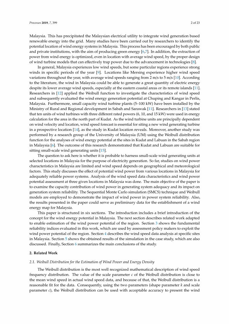
Abstract: This paper presents a statistical analysis of wind speed data that can be extremely usefulfor installing a wind generation as a stand-alone system. The main objective is to define the windpower capacity’s contribution to the adequacy of generation systems for the purpose of selectingwind farm locations at specific sites in Malaysia. The combined Sequential Monte Carlo simulation(SMCS) technique and the Weibull distribution models are employed to demonstrate the impactof wind power in power system reliability. To study this, the Roy Billinton Test System (RBTS) isconsidered and tested using wind data from two sites in Peninsular Malaysia, Mersing and KualaTerengganu, and one site, Kudat, in Sabah. The results showed that Mersing and Kudat were bestsuitable for wind sites. In addition, the reliability indices are compared prior to the addition of thetwo wind farms to the considered RBTS system. The results reveal that the reliability indices areslightly improved for the RBTS system with wind power generation from both the potential sites.

Keywords: reliability indices; wind farms; Sequential Monte Carlo Simulation; Malaysia

1. Introduction

Recent environmental impacts and the depletion of fossil fuel reserves are the main concerns thathave stimulated the integration of renewable energy power plants using solar power, wind power,biomass, biogas, etc. as alternative sources of electrical generation. This has inspired global concernsin energy balance, sustainability, security, and environmental preservation [1].

Wind energy is non-depletable, free, environmentally friendly, and almost available globally [2].It is intermittent, though very reliable from a long-term energy policy viewpoint [3]. In the measure ofadequacy, wind energy is regarded as a better choice compared with other energies.

Electric power systems continue to witness the penetration of high-level wind power into thesystem as a global phenomenon [4], due to the problems associated with power system planningand operation. This makes the assessment of wind power generation system capacities, and theirimpacts on reliability in the system by appropriate planning, in line with their power utilization andenvironmental benefits. Thus, high penetration of intermittent wind energy resources into the electricpower system requires the need to investigate the system reliability while adding a large amount ofvarying wind power generation to the system [5].

Owing to the industrial development and growth in the economy, an increase in the demandfor electricity is one of the major challenges faced by both developed and developing countries like

Processes 2019, 7, 399; doi:10.3390/pr7070399 www.mdpi.com/journal/processes

http://www.mdpi.com/journal/processes

http://www.mdpi.com

https://orcid.org/0000-0002-9042-9796

http://dx.doi.org/10.3390/pr7070399

http://www.mdpi.com/journal/processes

https://www.mdpi.com/2227-9717/7/7/399?type=check_update&version=2

Processes 2019, 7, 399 2 of 23

Malaysia. This has precipitated the Malaysian electrical utility to integrate wind generation basedrenewable energy into the grid. Many studies have been carried out by researchers to identify thepotential location of wind energy systems in Malaysia. This process has been encouraged by both publicand private institutions, with the aim of producing green energy [6,7]. In addition, the extraction ofpower from wind energy is optimized, even in location with average wind speed, by the proper designof wind turbine models that can effectively trap power due to the advancement in technologies [8].

In general, Malaysia experiences low wind speeds, but some particular regions experience strongwinds in specific periods of the year [9]. Locations like Mersing experience higher wind speedvariations throughout the year, with average wind speeds ranging from 2 m/s to 5 m/s [10]. Accordingto the literature, the wind in Malaysia could be able to generate a great quantity of electric energydespite its lower average wind speeds, especially at the eastern coastal areas or its remote islands [11].Researchers in [12] applied the Weibull function to investigate the characteristics of wind speedand subsequently evaluated the wind energy generation potential at Chuping and Kangar in Perlis,Malaysia. Furthermore, small capacity wind turbine plants (5–100 kW) have been installed by theMinistry of Rural and Regional development in Sabah and Sarawak [11]. Researchers in [13] statedthat ten units of wind turbines with three different rated powers (6, 10, and 15 kW) were used in energycalculation for the area in the north part of Kudat. As the wind turbine units are principally dependenton wind velocity and location, wind speed forecast is essential for siting a new wind generating turbinein a prospective location [14], as the study in Kudat location reveals. Moreover, another study wasperformed by a research group of the University of Malaysia (UM) using the Weibull distributionfunction for the analyses of wind energy potential at the sites in Kudat and Labuan in the Sabah regionin Malaysia [6]. The outcome of this research demonstrated that Kudat and Labuan are suitable forsitting small-scale wind generating units [15].

The question to ask here is whether it is probable to harness small-scale wind generating units atselected locations in Malaysia for the purpose of electricity generation. So far, studies on wind powercharacteristics in Malaysia are limited and wind speed depends on geographical and meteorologicalfactors. This study discusses the effect of potential wind power from various locations in Malaysia foradequately reliable power systems. Analysis of the wind speed data characteristics and wind powerpotential assessment at three given locations in Malaysia was done. The main objective of the paper isto examine the capacity contribution of wind power in generating system adequacy and its impact ongeneration system reliability. The Sequential Monte Carlo simulation (SMCS) technique and Weibullmodels are employed to demonstrate the impact of wind power in power system reliability. Also,the results presented in the paper could serve as preliminary data for the establishment of a windenergy map for Malaysia.

This paper is structured in six sections. The introduction includes a brief introduction of theconcept for the wind energy potential in Malaysia. The next section describes related work adaptedto enable estimation of the wind power potential of the region. Section 3 shows the fundamentalreliability indices evaluated in this work, which are used by assessment policy makers to exploit thewind power potential of the region. Section 4 describes the wind speed data analysis at specific sitesin Malaysia. Section 5 shows the obtained results of the simulation in the case study, which are alsodiscussed. Finally, Section 6 summarizes the main conclusions of the study.

2. Related Work

2.1. Weibull Distribution for the Estimation of Wind Power and Energy Density

The Weibull distribution is the most well recognized mathematical description of wind speedfrequency distribution. The value of the scale parameter c of the Weibull distribution is close tothe mean wind speed in actual wind speed data, and because of that, the Weibull distribution is areasonable fit for the data. Consequently, using the two parameters (shape parameter k and scaleparameter c), the Weibull distribution can be used with acceptable accuracy to present the wind

Processes 2019, 7, 399 3 of 23

speed frequency distribution and to predict wind power output from wind energy conversion system(WECS) [16].

Many numerical methods are employed to estimate the values of the shape parameter k and scalec. The Empirical Method (EM) is used in this paper for calculating the Weibull parameters. The EMcan be calculated by employing mean wind speed and the standard deviation, where the Weibullparameters c and k are given by the following equations [17].

k =

(σ

Processes 2019, 7, x FOR PEER REVIEW 3 of 26

in Malaysia. Section 5 shows the obtained results of the simulation in the case study, which are also discussed. Finally, Section 6 summarizes the main conclusions of the study.

2. Related Work


The Weibull distribution is the most well recognized mathematical description of wind speed frequency distribution. The value of the scale parameter c of the Weibull distribution is close to the mean wind speed in actual wind speed data, and because of that, the Weibull distribution is a reasonable fit for the data. Consequently, using the two parameters (shape parameter k and scale parameter c), the Weibull distribution can be used with acceptable accuracy to present the wind speed frequency distribution and to predict wind power output from wind energy conversion system (WECS) [16].

Many numerical methods are employed to estimate the values of the shape parameter k and scale c. The Empirical Method (EM) is used in this paper for calculating the Weibull parameters. The EM can be calculated by employing mean wind speed and the standard deviation, where the Weibull parameters c and k are given by the following equations [17].

𝑘 = 𝜎 ⊽ . (1) 𝑐 = ⊽┌(1 + 1 𝑘) (2)

where 𝜎 is standard deviation, ⊽ is the mean wind speed, ┌ is the gamma function, and k can be determined easily from the values of 𝜎 and ⊽, which are computed from the wind speed data set provided with the following formulation [18].

⊽= 1𝑛 𝑣 (3)

𝜎 = 1𝑛 − 1 (𝑣 −⊽) (4)

where ⊽ is the mean wind speed (m/s), n is the number of measured data, 𝑣 is wind speed of the observed data in the form of time series of wind speed (m/s), and 𝜎 is standard deviation. Once k is obtained from the solution of the above numerical expression (1), the scale factor c can be calculated by the above Equation (2).

Wind power density is a beneficial way of evaluating wind source availability at a potential height. It indicates the quantity of energy that can be used for conversion by a wind turbine [19]. The power that is available in the wind flowing at mean speed, ⊽, through a wind rotor blade with sweep area, An (m2), at any particular site can be projected as

𝑃(𝑣) = 12 𝜌𝐴(⊽) .

The monthly or annual mean wind power density per unit area of any site on the basis of a Weibull probability density function can be displayed in [20] as follows:

𝑃 (𝑤) = 𝑝(𝑣)𝐴 = 12 𝜌𝑐 ┌ 1 + 3𝑘 (5)

)−1.089

(1)

c =



2. Related Work




𝑘 = 𝜎 ⊽ . (1) 𝑐 = ⊽┌(1 + 1 𝑘) (2)


⊽= 1𝑛 𝑣 (3)

𝜎 = 1𝑛 − 1 (𝑣 −⊽) (4)



𝑃(𝑣) = 12 𝜌𝐴(⊽) .


𝑃 (𝑤) = 𝑝(𝑣)𝐴 = 12 𝜌𝑐 ┌ 1 + 3𝑘 (5)



2. Related Work




𝑘 = 𝜎 ⊽ . (1) 𝑐 = ⊽┌(1 + 1 𝑘) (2)


⊽= 1𝑛 𝑣 (3)

𝜎 = 1𝑛 − 1 (𝑣 −⊽) (4)



𝑃(𝑣) = 12 𝜌𝐴(⊽) .


𝑃 (𝑤) = 𝑝(𝑣)𝐴 = 12 𝜌𝑐 ┌ 1 + 3𝑘 (5)

(1 + 1

k

) (2)

where σ is standard deviation,



2. Related Work




𝑘 = 𝜎 ⊽ . (1) 𝑐 = ⊽┌(1 + 1 𝑘) (2)


⊽= 1𝑛 𝑣 (3)

𝜎 = 1𝑛 − 1 (𝑣 −⊽) (4)



𝑃(𝑣) = 12 𝜌𝐴(⊽) .


𝑃 (𝑤) = 𝑝(𝑣)𝐴 = 12 𝜌𝑐 ┌ 1 + 3𝑘 (5)

is the mean wind speed,



2. Related Work




𝑘 = 𝜎 ⊽ . (1) 𝑐 = ⊽┌(1 + 1 𝑘) (2)


⊽= 1𝑛 𝑣 (3)

𝜎 = 1𝑛 − 1 (𝑣 −⊽) (4)



𝑃(𝑣) = 12 𝜌𝐴(⊽) .


𝑃 (𝑤) = 𝑝(𝑣)𝐴 = 12 𝜌𝑐 ┌ 1 + 3𝑘 (5)

is the gamma function, and k can be

determined easily from the values of σ and



2. Related Work




𝑘 = 𝜎 ⊽ . (1) 𝑐 = ⊽┌(1 + 1 𝑘) (2)


⊽= 1𝑛 𝑣 (3)

𝜎 = 1𝑛 − 1 (𝑣 −⊽) (4)



𝑃(𝑣) = 12 𝜌𝐴(⊽) .


𝑃 (𝑤) = 𝑝(𝑣)𝐴 = 12 𝜌𝑐 ┌ 1 + 3𝑘 (5)

, which are computed from the wind speed data setprovided with the following formulation [18].



2. Related Work




𝑘 = 𝜎 ⊽ . (1) 𝑐 = ⊽┌(1 + 1 𝑘) (2)


⊽= 1𝑛 𝑣 (3)

𝜎 = 1𝑛 − 1 (𝑣 −⊽) (4)



𝑃(𝑣) = 12 𝜌𝐴(⊽) .


𝑃 (𝑤) = 𝑝(𝑣)𝐴 = 12 𝜌𝑐 ┌ 1 + 3𝑘 (5)

=1n

n∑i=1

vi (3)

σ =

1n− 1

n∑i=1

(vi −



2. Related Work




𝑘 = 𝜎 ⊽ . (1) 𝑐 = ⊽┌(1 + 1 𝑘) (2)


⊽= 1𝑛 𝑣 (3)

𝜎 = 1𝑛 − 1 (𝑣 −⊽) (4)



𝑃(𝑣) = 12 𝜌𝐴(⊽) .


𝑃 (𝑤) = 𝑝(𝑣)𝐴 = 12 𝜌𝑐 ┌ 1 + 3𝑘 (5)

)2

12

(4)

where



2. Related Work




𝑘 = 𝜎 ⊽ . (1) 𝑐 = ⊽┌(1 + 1 𝑘) (2)


⊽= 1𝑛 𝑣 (3)

𝜎 = 1𝑛 − 1 (𝑣 −⊽) (4)



𝑃(𝑣) = 12 𝜌𝐴(⊽) .


𝑃 (𝑤) = 𝑝(𝑣)𝐴 = 12 𝜌𝑐 ┌ 1 + 3𝑘 (5)

is the mean wind speed (m/s), n is the number of measured data, vi is wind speed of theobserved data in the form of time series of wind speed (m/s), and σ is standard deviation. Once k isobtained from the solution of the above numerical expression (1), the scale factor c can be calculated bythe above Equation (2).

Wind power density is a beneficial way of evaluating wind source availability at a potential height.It indicates the quantity of energy that can be used for conversion by a wind turbine [19]. The power

that is available in the wind flowing at mean speed,



2. Related Work




𝑘 = 𝜎 ⊽ . (1) 𝑐 = ⊽┌(1 + 1 𝑘) (2)


⊽= 1𝑛 𝑣 (3)

𝜎 = 1𝑛 − 1 (𝑣 −⊽) (4)



𝑃(𝑣) = 12 𝜌𝐴(⊽) .


𝑃 (𝑤) = 𝑝(𝑣)𝐴 = 12 𝜌𝑐 ┌ 1 + 3𝑘 (5)

, through a wind rotor blade with sweep area,An (m2), at any particular site can be projected as

P(v) =12ρA

(



2. Related Work




𝑘 = 𝜎 ⊽ . (1) 𝑐 = ⊽┌(1 + 1 𝑘) (2)


⊽= 1𝑛 𝑣 (3)

𝜎 = 1𝑛 − 1 (𝑣 −⊽) (4)



𝑃(𝑣) = 12 𝜌𝐴(⊽) .


𝑃 (𝑤) = 𝑝(𝑣)𝐴 = 12 𝜌𝑐 ┌ 1 + 3𝑘 (5)

)3.

The monthly or annual mean wind power density per unit area of any site on the basis of a Weibullprobability density function can be displayed in [20] as follows:

PD(w) =p(v)

A=

12ρc3

(1 +

3k

)(5)

where p(v) is the wind power (Watts), PD(w) is the mean wind power density (Watts/m2), ρ is the

air density at the site (1.225 kg/m3), A is the sweep area of the rotor blades (m2), and



2. Related Work




𝑘 = 𝜎 ⊽ . (1) 𝑐 = ⊽┌(1 + 1 𝑘) (2)


⊽= 1𝑛 𝑣 (3)

𝜎 = 1𝑛 − 1 (𝑣 −⊽) (4)



𝑃(𝑣) = 12 𝜌𝐴(⊽) .


𝑃 (𝑤) = 𝑝(𝑣)𝐴 = 12 𝜌𝑐 ┌ 1 + 3𝑘 (5)

(x) is thegamma function.

The extractible mean energy density over a time period (T) is calculated as

ED =12ρc3



2. Related Work




𝑘 = 𝜎 ⊽ . (1) 𝑐 = ⊽┌(1 + 1 𝑘) (2)


⊽= 1𝑛 𝑣 (3)

𝜎 = 1𝑛 − 1 (𝑣 −⊽) (4)



𝑃(𝑣) = 12 𝜌𝐴(⊽) .


𝑃 (𝑤) = 𝑝(𝑣)𝐴 = 12 𝜌𝑐 ┌ 1 + 3𝑘 (5)

(1 +

3k

)T (6)

where the time period (T) is expressed a daily, monthly or annual.

Processes 2019, 7, 399 4 of 23

2.2. Estimation of Wind Turbine Output Power and Capacity Factor

The performance of how a wind machine located in a site performs can be assessed as mean poweroutput Pe,ave over a specific time frame and capacity factor, Cf, of the wind machine. Pe,ave determinesthe total energy production and total income, whereas Cf is a ratio of the mean power output tothe rated electrical power Prated of the chosen wind turbine model [21]. Depending on the Weibulldistribution parameters, the Pe,ave and capacity factor Cf of a wind machine are computed according tothe following equations.

Pe,ave = Prated

e−(Vcc )

k− e−(

Vrc )

k(Vrc

)k−

(Vcc

)k

− e−(Vcc )

k

(7)

C f =Pe,ave

Prated(8)

where Vc is cut-in wind speed and Vr is the rated wind speed of the wind turbine generator (WTG).For an economical and viable investment in wind power, it is advisable that the capacity factor shouldexceed 25% and be maintained in the range of 25–45% [22].

2.3. Extrapolation of Wind Speed at Different Heights

Indirect wind speed estimation methods consist of measuring wind speed at a lower height andapplying an extrapolation model to estimate the wind speed characterization at different elevations.The most commonly used model is the power law [23].

Wind speed increases significantly with the height above ground level, depending on the roughnessof the terrain. Therefore, correct wind speed measurements must consider the hub height (H) for theWTG and the roughness of the terrain of the wind site. If measurements are difficult at high elevations,the standard wind speed height extrapolation formula, as in the power law Equation (9) [24], can beused to estimate wind speed at high elevations by using wind speed measured at a lower referenceelevation, typically 10 m [25].

v = vo

[H

HO

]n

(9)

where v is the wind speed estimated at desired height, H; vo is the wind speed reference hub height Ho,and (n) is the ground surface friction coefficient. The exponent (n) is dependent on factors such assurface roughness and atmospheric stability. Numerically, it ranges from (0.05–0.5) [26]. The normalvalue of ground surface for every station is approximated 1/7 or 0.143, as suggested by [27] for neutralstability conditions.

3. Reliability Assessment for Generation Systems

3.1. Fundamental Reliability Indices

The Load and generation models are conjoined to produce the risk model of the system. Indicesthat evaluate system reliability and adequacy can be used to forecast the reliability of the powergenerating system.

The fundamental reliability indices evaluated in this work are adapted to enable the estimationof the reliability level of the power generating systems, comprised of Loss of Load Frequency(LOLF), Loss of Energy Expectation (LOEE), Loss of Load Duration (LOLD), and Loss of LoadExpectation (LOLE).

At present, LOLE represents the reliability index of the electrical power systems used in manycountries [3]. The standard level of LOLE is one-day-in ten years or less. This does not mean a fullday of shortages once every ten years; rather, it refers to the total accumulated time of shortages,which should not exceed one day in ten years. Therefore, the level of LOLE in this study is used as areliability index of the generation systems.

Processes 2019, 7, 399 5 of 23

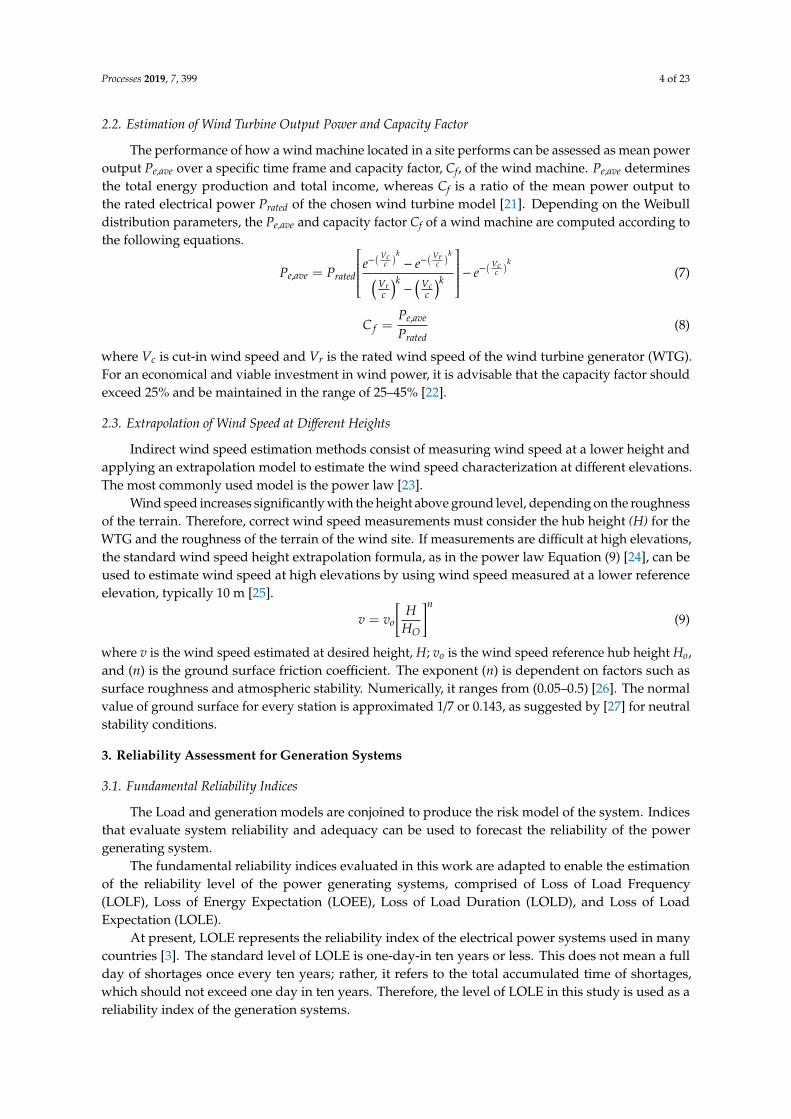
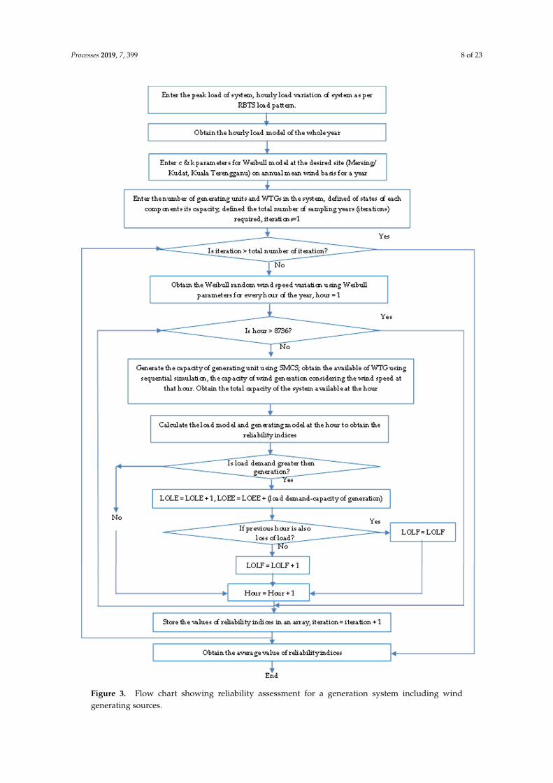
The combined Sequential Monte Carlo simulation (SMCS) method (or the Monte Carlo simulationmethod cooperate with Frequency and Duration method) in [28] enables accurate evaluation ofreliability indices. To accurately evaluate the reliability assessment for the overall reliability ofgenerating systems adequacy containing wind energy, an SMCS method was used alongside theWeibull distribution model to generate and repeat the wind speed. The Roy Billinton Test System(RBTS) is an essential reliability test system produced by the University of Saskatchewan (Canada) foreducational and research purposes. The RBTS has 11 conventional generating units, each having apower capacity ranging of around 5–40 MW, with an installed capacity of 240 MW and a peak load of185 MW. Figure 1 shows the single line diagram for the RBTS, and the detailed reliability data for thegenerating units in the test system are shown in Appendix A. The load model is generally representedas chronological Load Duration Curve (LDC), which is used along with different search techniques.The LDC will generate values for each hour, so there will be 8736 individual values recorded for eachyear. The chronological LDC hourly load model shown in Figure 2 was utilized, and the system peakload is 185 MW. Besides the traditional generators, the wind farm was comprised of 53 identical WTGunits with a rated power of 35 kW, each of which was considered in the current study. A peak load of1% penetrated wind energy in the RBTS system, which has a peak load of 185 MW.


The Load and generation models are conjoined to produce the risk model of the system. Indices

that evaluate system reliability and adequacy can be used to forecast the reliability of the power

generating system.

The fundamental reliability indices evaluated in this work are adapted to enable the estimation

of the reliability level of the power generating systems, comprised of Loss of Load Frequency (LOLF),

Loss of Energy Expectation (LOEE), Loss of Load Duration (LOLD), and Loss of Load Expectation

(LOLE).

At present, LOLE represents the reliability index of the electrical power systems used in many

countries [3]. The standard level of LOLE is one-day-in ten years or less. This does not mean a full

day of shortages once every ten years; rather, it refers to the total accumulated time of shortages,

which should not exceed one day in ten years. Therefore, the level of LOLE in this study is used as a

reliability index of the generation systems.

The combined Sequential Monte Carlo simulation (SMCS) method (or the Monte Carlo

simulation method cooperate with Frequency and Duration method) in [28] enables accurate

evaluation of reliability indices. To accurately evaluate the reliability assessment for the overall

reliability of generating systems adequacy containing wind energy, an SMCS method was used

alongside the Weibull distribution model to generate and repeat the wind speed. The Roy Billinton

Test System (RBTS) is an essential reliability test system produced by the University of Saskatchewan

(Canada) for educational and research purposes. The RBTS has 11 conventional generating units,

each having a power capacity ranging of around 5–40 MW, with an installed capacity of 240 MW and

a peak load of 185 MW. Figure 1 shows the single line diagram for the RBTS, and the detailed

reliability data for the generating units in the test system are shown in Appendix A. The load model

is generally represented as chronological Load Duration Curve (LDC), which is used along with

different search techniques. The LDC will generate values for each hour, so there will be 8736

individual values recorded for each year. The chronological LDC hourly load model shown in Figure

2 was utilized, and the system peak load is 185 MW. Besides the traditional generators, the wind farm

was comprised of 53 identical WTG units with a rated power of 35 kW, each of which was considered

in the current study. A peak load of 1% penetrated wind energy in the RBTS system, which has a

peak load of 185 MW.

Figure 1. Single line diagrams of the Roy Billinton Test System (RBTS). Figure 1. Single line diagrams of the Roy Billinton Test System (RBTS).Processes 2019, 7, x FOR PEER REVIEW 6 of 26

Figure 2. Chronological hourly load (Load Duration Curve (LDC)) model for the RBTS.

3.2. Proposed Methodology

The basic simulation procedures for applying the SMCS with the Weibull model in calculating

reliability indices for the electrical power generating systems with wind energy penetration are based

on the following steps.

Step 1: The generation of the yearly synthetic wind power time series employs a Weibull model,

as follows:

• Set the Weibull distribution parameters k and c.

• Generate a uniformly distributed random number U between (0,1).

• Determined the artificial wind speed v with Equation (10).

� = �[− �� (�)��] (10)

• Set the WTG’s Vci, Vr, and Vco wind speeds.

• Determine the constants A, Bx, and Cx with the equations below.

� =1

(�� − ��)�� (�� + ��)− 4��

�� + ��

2��

��

�

�� =1

(�� − ��)��4 (�� + ��) �

�� + ��

2��

��

− (3�� + ��)�

�� =1

(�� − ��)��2 − 4 �

�� + ��

2��

��

�.

• Calculate the WTG output power using Equation (11),

co

corr

rcirx

ci

WTG

Vws

VwsVP

VwsVPCxBA

Vws

P

0

)(

02

(11)

Figure 2. Chronological hourly load (Load Duration Curve (LDC)) model for the RBTS.

Processes 2019, 7, 399 6 of 23

3.2. Proposed Methodology

The basic simulation procedures for applying the SMCS with the Weibull model in calculatingreliability indices for the electrical power generating systems with wind energy penetration are basedon the following steps.

Step 1: The generation of the yearly synthetic wind power time series employs a Weibull model,as follows:

• Set the Weibull distribution parameters k and c.• Generate a uniformly distributed random number U between (0,1).• Determined the artificial wind speed v with Equation (10).

v = c[− ln(U)

1k

](10)

• Set the WTG’s Vci, Vr, and Vco wind speeds.• Determine the constants A, Bx, and Cx with the equations below.

A =1

(Vci −Vr)2

{Vci (Vci + Vr) − 4VciVr

[Vci + Vr

2Vr

]3}

Bx =1

(Vci −Vr)2

{4 (Vci + Vr)

[Vci + Vr

2Vr

]3− (3Vci + Vr)

}

Cx =1

(Vci −Vr)2

{2− 4

[Vci + Vr

2Vr

]3}.

• Calculate the WTG output power using Equation (11),

PWTG =

0 ws < Vci(A + Bx + Cx2) × Pr Vci ≤ ws < Vr

Pr Vr ≤ ws < Vco

0 ws > Vco

(11)

where ws = wind speed (m/s), Vci = WTG cut-in speed (m/s), Vco = WTG cut-out speed (m/s),Vr = WTG rated speed (m/s), and Pr = WTG rated power output (MW). The constants A, Bx,and Cx have previously been calculated by [3].

Step 2: Create the total available capacity generation by a combination of the synthetic generatedwind power time series with a conventional chronological generating system model by employingSMCS, as follows:

• Define the maximum number of years (N) to be simulated and set the simulation time (h),(usually one year) to run with SMCS.

• Generate uniform random numbers for the operation cycle (up-down-up) for each of theconventional units in the system by using the unit’s annual MTTR (mean time to repair) and λ

(failure rate) values.• The component’s sequential state transition processes within the time of all components are then

added to create the sequential system state.• Define the system capacity by aggregating the available capacities of all system components

by combining the operating cycles of generating units and the operating cycles with the WTGavailable hourly wind at a given load level.

Processes 2019, 7, 399 7 of 23

• Superimpose the available system capacity curve on the sequential hourly load curve to obtainthe available system margin. A positive margin denotes sufficient system generation to meet thesystem load whereas a negative margin suggests system load shedding.

• The reliability indices for a number of sample years (N) can be obtained using Equations (12)–(18).

ΦLOLE(s) ={

0 i f s j ∈ ssuccess

1 i f s j ∈ s f ailure(12)

E(ΦLOLE(s)) =

∑Ni=1

{∑nj(s)j=1 ΦLOLE(sji)

}N

(13)

where i = 1, 2 . . . N, N = number of years simulated, φ(sji) = index function analogous to jthoccurrence within the year i, j = 1, 2 . . . , nj(s), nj(s) is the number of system state occurrences of (sj)in the year i, sj = ssuccess


where ws = wind speed (m/s), Vci = WTG cut-in speed (m/s), Vco = WTG cut-out speed (m/s), Vr = WTG rated speed (m/s), and Pr = WTG rated power output (MW). The constants A, Bx, and Cx have previously been calculated by [3].

Step 2: Create the total available capacity generation by a combination of the synthetic generated wind power time series with a conventional chronological generating system model by employing SMCS, as follows:

• Define the maximum number of years (N) to be simulated and set the simulation time (h), (usually one year) to run with SMCS.

• Generate uniform random numbers for the operation cycle (up-down-up) for each of the conventional units in the system by using the unit’s annual MTTR (mean time to repair) and λ (failure rate) values.

• The component’s sequential state transition processes within the time of all components are then added to create the sequential system state.

• Define the system capacity by aggregating the available capacities of all system components by combining the operating cycles of generating units and the operating cycles with the WTG available hourly wind at a given load level.

• Superimpose the available system capacity curve on the sequential hourly load curve to obtain the available system margin. A positive margin denotes sufficient system generation to meet the system load whereas a negative margin suggests system load shedding.

• The reliability indices for a number of sample years (N) can be obtained using Equations (12)–(18).

Ф (𝑠) = 0 𝑖𝑓 𝑠𝑗 ∈ 𝑠1 𝑖𝑓 𝑠𝑗 ∈ 𝑠 (12)

Ẽ(Ф (𝑠)) = ∑ ∑ Ф( ) (𝑠𝑗𝑖)𝑁 (13)

where i = 1, 2… N, N = number of years simulated, Ф(sji) = index function analogous to jth occurrence within the year i, j = 1, 2…, nj(s), nj(s) is the number of system state occurrences of (sj) in the year i, sj = ssuccess ᴜ sfailure is the set of all possible states (sj) (i.e., the state-space), and the content of two subspaces ssucess of the success state and sfailure of the failure states.

Ф (𝑠) = 0 𝑖𝑓 𝑠𝑗 ∈ 𝑠∆𝑃𝑗 × 𝑇 𝑖𝑓 𝑠𝑗 ∈ 𝑠 (14)

Ẽ(Ф (𝑠)) = ∑ ∑ Ф( ) (𝑠𝑗𝑖)𝑁 (55)

where ∆Pj×T is the amount of curtailing energy in the failed state (sji).

Ф (𝑠) = 0 𝑖𝑓 𝑠𝑗 ∈ 𝑠∆𝜆𝑗 𝑖𝑓 𝑠𝑗 ∈ 𝑠 (16)

Ẽ(Ф (𝑠)) = ∑ ∑ Ф( ) (𝑠𝑗𝑖)𝑁 . (17)

∆λj, is the sum of the transition rates between sj and all the ssuccess states attained from sj in one transition.

sfailure is the set of all possible states (sj) (i.e., the state-space), and thecontent of two subspaces ssucess of the success state and sfailure of the failure states.

ΦLOEE(s) ={


∆Pj× T i f s j ∈ s f ailure(14)

E(ΦLOEE(s)) =

∑Ni=1

{∑nj(s)j=1 ΦLOEE(sji)

}N

(15)

where ∆Pj×T is the amount of curtailing energy in the failed state (sji).

ΦLOLF(s) ={


∆λ j i f s j ∈ s f ailure(16)

E(ΦLOLF(s)) =

∑Ni=1

{∑nj(s)j=1 ΦLOLF(sji)

}N

. (17)

∆λj, is the sum of the transition rates between sj and all the ssuccess states attained from sj inone transition.

LOLD =LOLELOLF

. (18)

• If (N) is equal to the maximum number of years, stop the simulation; otherwise, set (N = N + 1),(h = 0), then return to move 2 and repeat the attempt.

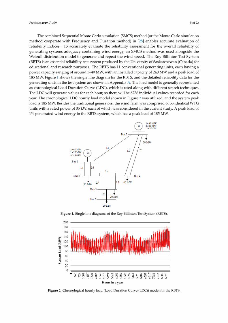
Step 3: Evaluate and update the outcome of the test function for the reliability indices evaluation.The above procedure is detailed in the form of flowchart, as represented in Figure 3.

Processes 2019, 7, 399 8 of 23


Figure 3. Flow chart showing reliability assessment for a generation system including wind

generating sources.

4. Wind Speed Data Analysis at Specific Sites in Malaysia

Figure 3. Flow chart showing reliability assessment for a generation system including windgenerating sources.

Processes 2019, 7, 399 9 of 23

4. Wind Speed Data Analysis at Specific Sites in Malaysia

To estimate the possible potential wind energy site in Malaysia, the analysis, correlation,and prediction of wind data from the location need to be done. It has been often recommended inthe literature that making use of the wind data available from meteorological stations increases thevicinity of the proposed candidate site by preliminary estimates of the wind resource potential ofthe site. Meteorological data that are recorded for long periods need to be extrapolated to obtainan estimation of the wind profile of the site. In this study, wind speed data from Mersing, Kudat,and Kuala Terengganu have been statistically analyzed to propose the wind energy characteristicsfor these sites. The data for this study were gathered from the Malaysia Meteorological Department(MMD). The data recorded comprise three years of hourly mean surface wind speeds from 2013 to2015 at three locations in Malaysia. The mean of the wind speed form the simulated process for eachhour is calculated based on Weibull parameters. The hourly mean wind speed is then used in thesequential simulation process. Figure 4 shows the locations of MMD stations in Peninsular Malaysia.This map was drawn by using the Arc Graphical Information System (AGIS) software and depictsthe strength of the wind speed distribution in Mersing, Kudat, and Kuala Terengganu. The area thatshowed the highest wind speed value is in red and orange, while other areas show moderate windspeeds. Table 1 presents a description of the selected regions in Malaysia, which consist of the latitude,longitude, and elevation of the anemometer.


To estimate the possible potential wind energy site in Malaysia, the analysis, correlation, and

prediction of wind data from the location need to be done. It has been often recommended in the

literature that making use of the wind data available from meteorological stations increases the

vicinity of the proposed candidate site by preliminary estimates of the wind resource potential of the

site. Meteorological data that are recorded for long periods need to be extrapolated to obtain an

estimation of the wind profile of the site. In this study, wind speed data from Mersing, Kudat, and

Kuala Terengganu have been statistically analyzed to propose the wind energy characteristics for

these sites. The data for this study were gathered from the Malaysia Meteorological Department

(MMD). The data recorded comprise three years of hourly mean surface wind speeds from 2013 to

2015 at three locations in Malaysia. The mean of the wind speed form the simulated process for each

hour is calculated based on Weibull parameters. The hourly mean wind speed is then used in the

sequential simulation process. Figure 4 shows the locations of MMD stations in Peninsular Malaysia.

This map was drawn by using the Arc Graphical Information System (AGIS) software and depicts

the strength of the wind speed distribution in Mersing, Kudat, and Kuala Terengganu. The area that

showed the highest wind speed value is in red and orange, while other areas show moderate wind

speeds. Table 1 presents a description of the selected regions in Malaysia, which consist of the

latitude, longitude, and elevation of the anemometer.

Figure 4. Wind speed distribution maps for station sites used in this study in Malaysia.

Table 1. Description of the wind speed stations at selected regions in Malaysia.

Station Latitude Longitude Altitude (m)

Mersing 2° 27′ N 103° 50′ E 43.6

Kuala Terengganu 5° 23′ N 103° 06′ E 5.2

Kudat 6° 55′ N 116° 50′ E 3.5

4.1. Estimation of Average Wind Speed with Different Height

Figure 4. Wind speed distribution maps for station sites used in this study in Malaysia.

Table 1. Description of the wind speed stations at selected regions in Malaysia.

Station Latitude Longitude Altitude (m)

Mersing 2◦27′ N 103◦50′ E 43.6Kuala Terengganu 5◦23′ N 103◦06′ E 5.2

Kudat 6◦55′ N 116◦50′ E 3.5

Processes 2019, 7, 399 10 of 23

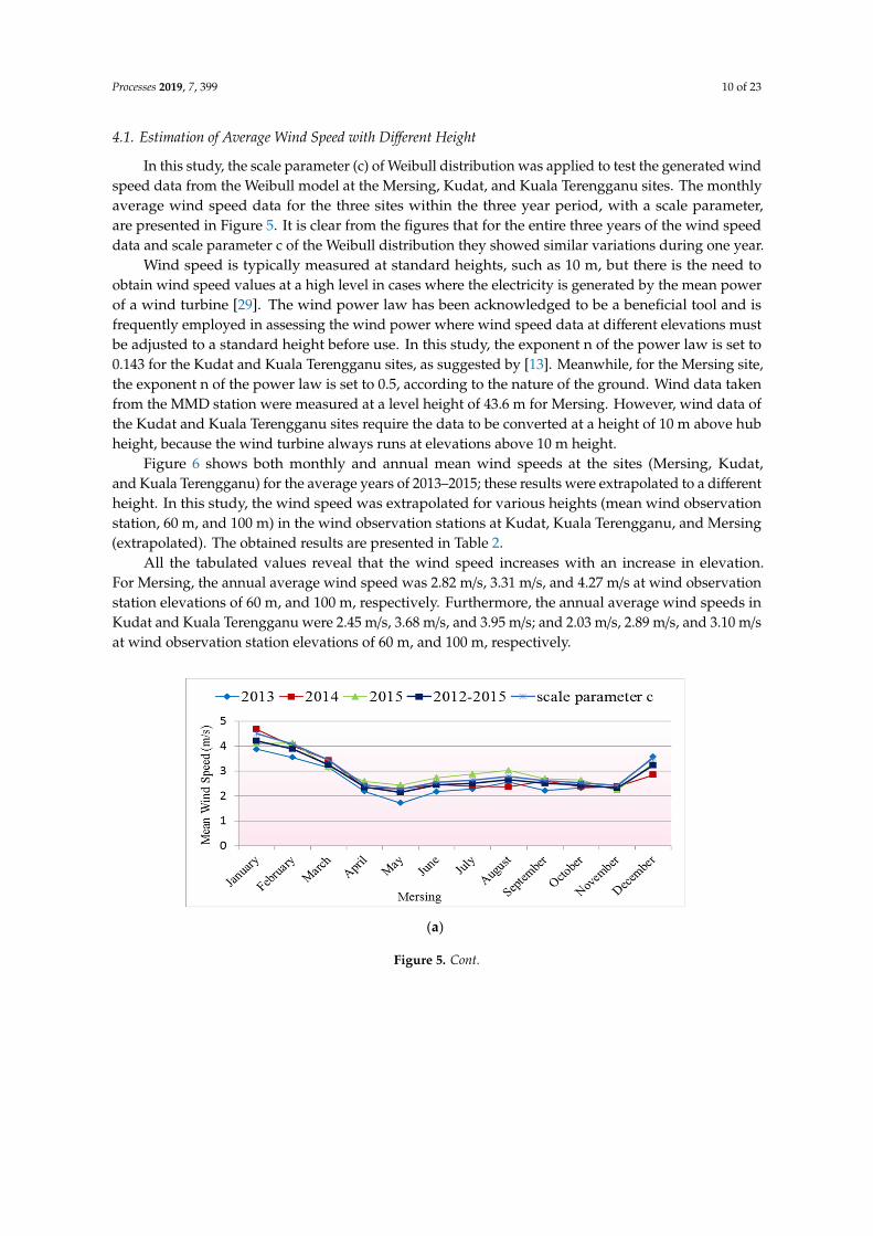
4.1. Estimation of Average Wind Speed with Different Height

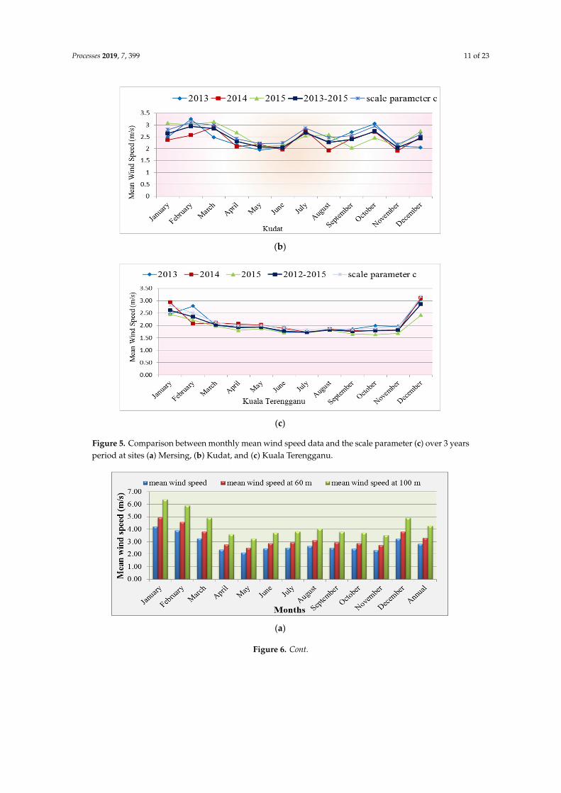
In this study, the scale parameter (c) of Weibull distribution was applied to test the generated windspeed data from the Weibull model at the Mersing, Kudat, and Kuala Terengganu sites. The monthlyaverage wind speed data for the three sites within the three year period, with a scale parameter,are presented in Figure 5. It is clear from the figures that for the entire three years of the wind speeddata and scale parameter c of the Weibull distribution they showed similar variations during one year.

Wind speed is typically measured at standard heights, such as 10 m, but there is the need toobtain wind speed values at a high level in cases where the electricity is generated by the mean powerof a wind turbine [29]. The wind power law has been acknowledged to be a beneficial tool and isfrequently employed in assessing the wind power where wind speed data at different elevations mustbe adjusted to a standard height before use. In this study, the exponent n of the power law is set to0.143 for the Kudat and Kuala Terengganu sites, as suggested by [13]. Meanwhile, for the Mersing site,the exponent n of the power law is set to 0.5, according to the nature of the ground. Wind data takenfrom the MMD station were measured at a level height of 43.6 m for Mersing. However, wind data ofthe Kudat and Kuala Terengganu sites require the data to be converted at a height of 10 m above hubheight, because the wind turbine always runs at elevations above 10 m height.

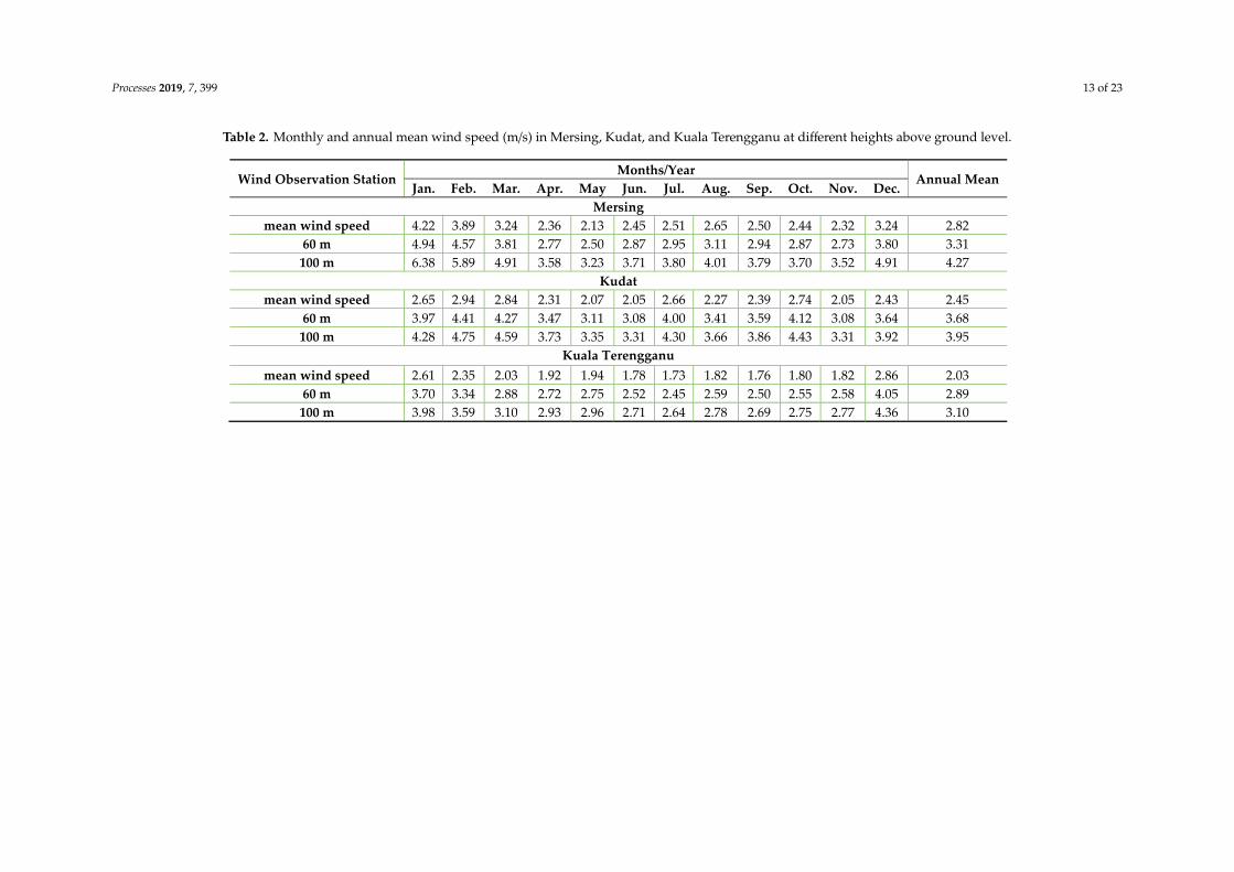
Figure 6 shows both monthly and annual mean wind speeds at the sites (Mersing, Kudat,and Kuala Terengganu) for the average years of 2013–2015; these results were extrapolated to a differentheight. In this study, the wind speed was extrapolated for various heights (mean wind observationstation, 60 m, and 100 m) in the wind observation stations at Kudat, Kuala Terengganu, and Mersing(extrapolated). The obtained results are presented in Table 2.

All the tabulated values reveal that the wind speed increases with an increase in elevation.For Mersing, the annual average wind speed was 2.82 m/s, 3.31 m/s, and 4.27 m/s at wind observationstation elevations of 60 m, and 100 m, respectively. Furthermore, the annual average wind speeds inKudat and Kuala Terengganu were 2.45 m/s, 3.68 m/s, and 3.95 m/s; and 2.03 m/s, 2.89 m/s, and 3.10 m/sat wind observation station elevations of 60 m, and 100 m, respectively.


In this study, the scale parameter (c) of Weibull distribution was applied to test the generated

wind speed data from the Weibull model at the Mersing, Kudat, and Kuala Terengganu sites. The

monthly average wind speed data for the three sites within the three year period, with a scale

parameter, are presented in Figure 5. It is clear from the figures that for the entire three years of the

wind speed data and scale parameter c of the Weibull distribution they showed similar variations

during one year.

Wind speed is typically measured at standard heights, such as 10 m, but there is the need to

obtain wind speed values at a high level in cases where the electricity is generated by the mean power

of a wind turbine [29]. The wind power law has been acknowledged to be a beneficial tool and is

frequently employed in assessing the wind power where wind speed data at different elevations must

be adjusted to a standard height before use. In this study, the exponent n of the power law is set to

0.143 for the Kudat and Kuala Terengganu sites, as suggested by [13]. Meanwhile, for the Mersing

site, the exponent n of the power law is set to 0.5, according to the nature of the ground. Wind data

taken from the MMD station were measured at a level height of 43.6 m for Mersing. However, wind

data of the Kudat and Kuala Terengganu sites require the data to be converted at a height of 10 m

above hub height, because the wind turbine always runs at elevations above 10 m height.

Figure 6 shows both monthly and annual mean wind speeds at the sites (Mersing, Kudat, and

Kuala Terengganu) for the average years of 2013–2015; these results were extrapolated to a different

height. In this study, the wind speed was extrapolated for various heights (mean wind observation

station, 60 m, and 100 m) in the wind observation stations at Kudat, Kuala Terengganu, and Mersing

(extrapolated). The obtained results are presented in Table 2.

All the tabulated values reveal that the wind speed increases with an increase in elevation. For

Mersing, the annual average wind speed was 2.82 m/s, 3.31 m/s, and 4.27 m/s at wind observation

station elevations of 60 m, and 100 m, respectively. Furthermore, the annual average wind speeds in

Kudat and Kuala Terengganu were 2.45 m/s, 3.68 m/s, and 3.95 m/s; and 2.03 m/s, 2.89 m/s, and 3.10

m/s at wind observation station elevations of 60 m, and 100 m, respectively.

(a)

Figure 5. Cont.

Processes 2019, 7, 399 11 of 23Processes 2019, 7, x FOR PEER REVIEW 12 of 26

(b)

(c)

Figure 5. Comparison between monthly mean wind speed data and the scale parameter (c) over 3

years period at sites (a) Mersing, (b) Kudat, and (c) Kuala Terengganu.

(a)

Figure 5. Comparison between monthly mean wind speed data and the scale parameter (c) over 3 yearsperiod at sites (a) Mersing, (b) Kudat, and (c) Kuala Terengganu.


(b)

(c)

Figure 5. Comparison between monthly mean wind speed data and the scale parameter (c) over 3

years period at sites (a) Mersing, (b) Kudat, and (c) Kuala Terengganu.

(a)

Figure 6. Cont.

Processes 2019, 7, 399 12 of 23Processes 2019, 7, x FOR PEER REVIEW 13 of 26

(b)

(c)

Figure 6. Monthly and annual mean wind speeds at sites (a) Mersing, (b) Kudat, and (c) Kuala

Terengganu.

4.2. Estimation of Wind Power Density and Energy Density at Different Heights

The observed wind speed data at the station were converted to 100 m height wind speed data

using Equation (9), and then the converted data were used to determine the wind potential. The scale

c and shape k Weibull parameters were estimated using the EM. The wind power and energy density

were measured, respectively, by Equations (5) and (6) at heights of (43.6 m) and (100 m) in Mersing,

as shown in Table 3. The rest of the calculations for wind power and energy density at heights of 3.5

and 100 m and 5.2 and 100 m in Kudat and Kuala Terengganu, respectively, can be found in Appendix

B.

From Table 3, it is observed that the maximum power density from the actual wind speed of

Mersing, Kudat, and Kuala Terengganu was found to be 52 W/m2, 19 W/m2, and 20 W/m2,

respectively. However, the maximum power density of Mersing, Kudat, and Kuala Terengganu,

when the actual wind speed data was converted to 100 m height, was calculated to be 180 W/m2, 80

W/m2, and 72 W/m2, respectively. Here, it is evident that the Mersing site has a higher mean monthly

power density compared to Kudat and Kala Terengganu under various heights.

Figure 6. Monthly and annual mean wind speeds at sites (a) Mersing, (b) Kudat, and (c)Kuala Terengganu.

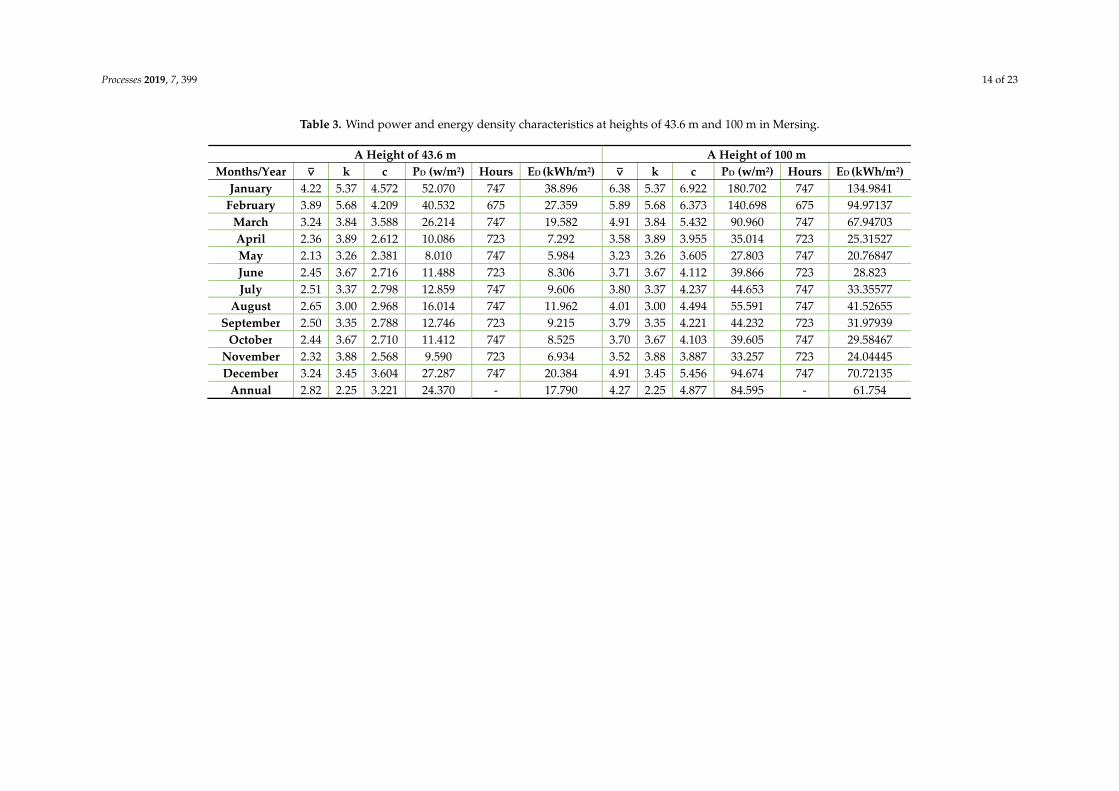
4.2. Estimation of Wind Power Density and Energy Density at Different Heights

The observed wind speed data at the station were converted to 100 m height wind speed datausing Equation (9), and then the converted data were used to determine the wind potential. The scale cand shape k Weibull parameters were estimated using the EM. The wind power and energy densitywere measured, respectively, by Equations (5) and (6) at heights of (43.6 m) and (100 m) in Mersing,as shown in Table 3. The rest of the calculations for wind power and energy density at heights of 3.5 and100 m and 5.2 and 100 m in Kudat and Kuala Terengganu, respectively, can be found in Appendix B.

From Table 3, it is observed that the maximum power density from the actual wind speed ofMersing, Kudat, and Kuala Terengganu was found to be 52 W/m2, 19 W/m2, and 20 W/m2, respectively.However, the maximum power density of Mersing, Kudat, and Kuala Terengganu, when the actualwind speed data was converted to 100 m height, was calculated to be 180 W/m2, 80 W/m2, and 72 W/m2,respectively. Here, it is evident that the Mersing site has a higher mean monthly power densitycompared to Kudat and Kala Terengganu under various heights.

Processes 2019, 7, 399 13 of 23

Table 2. Monthly and annual mean wind speed (m/s) in Mersing, Kudat, and Kuala Terengganu at different heights above ground level.


Table 2. Monthly and annual mean wind speed (m/s) in Mersing, Kudat, and Kuala Terengganu at different heights above ground level.

Wind Observation Station Months/Year

Annual Mean Jan. Feb. Mar. Apr. May Jun. Jul. Aug. Sep. Oct. Nov. Dec.

Mersing mean wind speed 4.22 3.89 3.24 2.36 2.13 2.45 2.51 2.65 2.50 2.44 2.32 3.24 2.82

60 m 4.94 4.57 3.81 2.77 2.50 2.87 2.95 3.11 2.94 2.87 2.73 3.80 3.31 100 m 6.38 5.89 4.91 3.58 3.23 3.71 3.80 4.01 3.79 3.70 3.52 4.91 4.27

Kudat mean wind speed 2.65 2.94 2.84 2.31 2.07 2.05 2.66 2.27 2.39 2.74 2.05 2.43 2.45

60 m 3.97 4.41 4.27 3.47 3.11 3.08 4.00 3.41 3.59 4.12 3.08 3.64 3.68 100 m 4.28 4.75 4.59 3.73 3.35 3.31 4.30 3.66 3.86 4.43 3.31 3.92 3.95

Kuala Terengganu mean wind speed 2.61 2.35 2.03 1.92 1.94 1.78 1.73 1.82 1.76 1.80 1.82 2.86 2.03

60 m 3.70 3.34 2.88 2.72 2.75 2.52 2.45 2.59 2.50 2.55 2.58 4.05 2.89 100 m 3.98 3.59 3.10 2.93 2.96 2.71 2.64 2.78 2.69 2.75 2.77 4.36 3.10

Processes 2019, 7, 399 14 of 23

Table 3. Wind power and energy density characteristics at heights of 43.6 m and 100 m in Mersing.


Table 3. Wind power and energy density characteristics at heights of 43.6 m and 100 m in Mersing.

A Height of 43.6 m A Height of 100 m Months/Year ⊽ k c PD (w/m2) Hours ED (kWh/m2) ⊽ k c PD (w/m2) Hours ED (kWh/m2)

January 4.22 5.37 4.572 52.070 747 38.896 6.38 5.37 6.922 180.702 747 134.9841 February 3.89 5.68 4.209 40.532 675 27.359 5.89 5.68 6.373 140.698 675 94.97137

March 3.24 3.84 3.588 26.214 747 19.582 4.91 3.84 5.432 90.960 747 67.94703 April 2.36 3.89 2.612 10.086 723 7.292 3.58 3.89 3.955 35.014 723 25.31527 May 2.13 3.26 2.381 8.010 747 5.984 3.23 3.26 3.605 27.803 747 20.76847 June 2.45 3.67 2.716 11.488 723 8.306 3.71 3.67 4.112 39.866 723 28.823 July 2.51 3.37 2.798 12.859 747 9.606 3.80 3.37 4.237 44.653 747 33.35577

August 2.65 3.00 2.968 16.014 747 11.962 4.01 3.00 4.494 55.591 747 41.52655 September 2.50 3.35 2.788 12.746 723 9.215 3.79 3.35 4.221 44.232 723 31.97939

October 2.44 3.67 2.710 11.412 747 8.525 3.70 3.67 4.103 39.605 747 29.58467 November 2.32 3.88 2.568 9.590 723 6.934 3.52 3.88 3.887 33.257 723 24.04445 December 3.24 3.45 3.604 27.287 747 20.384 4.91 3.45 5.456 94.674 747 70.72135

Annual 2.82 2.25 3.221 24.370 - 17.790 4.27 2.25 4.877 84.595 - 61.754

Processes 2019, 7, 399 15 of 23

The annual mean power density of Mersing, Kudat, and Kuala Terengganu varies between84.59 W/m2, 79.28 W/m2, and 33.36 W/m2 at a height of 100 m. The annual power density is also lessthan 100 W/m2 for all the locations, and, therefore, these locations can be categorized as a class 1 windenergy resource. This wind energy resource class, in general, is inappropriate for large-scale windturbine applications. Nevertheless, the generation of small-scale wind energy at a turbine height of100 m [6] is viable. However, for small-scale applications, and in the long-term with the developmentof wind turbine technology, the use of wind energy continues to hold great promise.

4.3. Estimation of the Suitable Wind Turbine Units at Malaysia Sites

The selection of the wind turbine should be made with a rated wind speed that corresponds tothe maximum energy wind speed in order to maximize energy output. For the annual energy output,the selected wind turbine will have the maximum capacity factor, defined by the ratio of the actualpower generated to the rated power output [30]. The average power output values, Pe,ave, and Cf,are crucial performance factors of the wind energy conversion system (WECS).

The technical data of six differently sized wind turbines are summarized in Table 4.The summarized information in Table 4 is obtained from [13,19]. The cut-in wind speed, or thespeed at which the turbine commences power production, is 2.7 m/s for four of the six turbines, whilefor the other two turbines, the cut-in wind speed values are 2 and 3.5 m/s, respectively. The cut-outwind speed of 25 m/s applies to all the turbines. Table 4 represents the information pertaining to therated speed, rated output power, hub height, and rotor diameter of the wind turbines analyzed.

Table 4. The technical data of wind turbines.

Characteristics P10-20 591672E P12-25 G-3120 P15-50 P25-100

Rated power (kw) 20 22 25 35 50 100Hub height (m) - 30 - 42.7 - -

Rotor diameter (m) 10 15 12 19.2 15.2 25Cut-in wind speed (m/s) 2.7 2 2.7 3.5 2.7 2.7Rated wind speed (m/s) 10 10 10 8 12 10

Cut-off wind speed (m/s) 25 25 25 25 25 25

Depending on the turbine’s characteristics in Table 4, and the Weibull parameters derived fromapplying EM using the Matlab toolbox, the electrical output of the wind turbines can be made availableby using the formulation earlier defined in Equation (7).

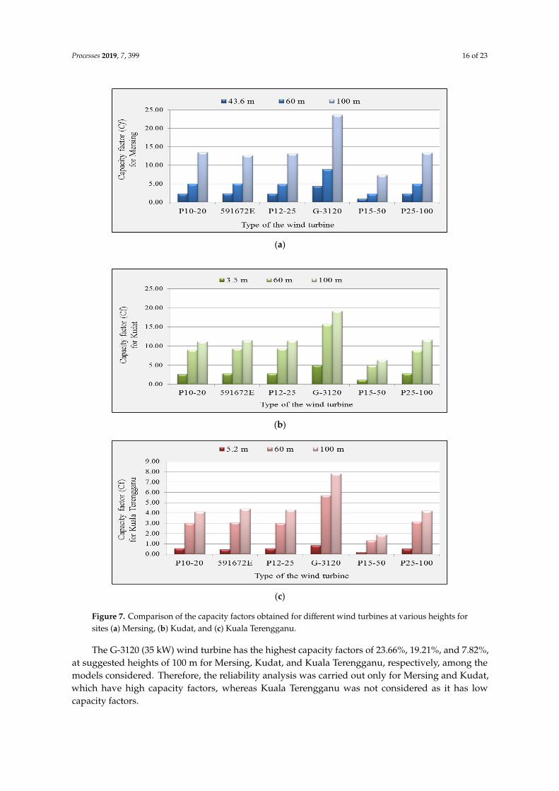
Knowing the output power of the wind turbines, it is then possible to obtain a computation of theaverage output power value of each wind turbine. As the capacity factor of a wind turbine is the ratioof its average output power to its rated power, the energy output data are employed in calculating thecapacity factor of the wind turbines, which are of sizes 20, 22, 25, 35, 50, and 100 kW. A comparison ofthe capacity factors computed for various wind turbines at different heights is presented in Figure 7.

From Figure 7, it can be seen that the capacity factor goes up as the hub height increases. Moreover,the capacity factor increases for wind turbines of a size of 35 kW. In Mersing, the maximum capacityfactor is achieved as about 23.66% for the Endurance America model of the G-3120 kW wind turbine,whereas in Kuala Terengganu, the lowest capacity factor is achieved as approximately 7.82% for theEndurance America model of the G-3120 kW wind turbine. Kudat, with about 19.21%, ranks second interms of capacity factors compared to the regions.

Processes 2019, 7, 399 16 of 23


for the Endurance America model of the G-3120 kW wind turbine. Kudat, with about 19.21%, ranks

second in terms of capacity factors compared to the regions.

(a)

(b)

(c)

Figure 7. Comparison of the capacity factors obtained for different wind turbines at various heights

for sites (a) Mersing, (b) Kudat, and (c) Kuala Terengganu.

Figure 7. Comparison of the capacity factors obtained for different wind turbines at various heights forsites (a) Mersing, (b) Kudat, and (c) Kuala Terengganu.

The G-3120 (35 kW) wind turbine has the highest capacity factors of 23.66%, 19.21%, and 7.82%,at suggested heights of 100 m for Mersing, Kudat, and Kuala Terengganu, respectively, among themodels considered. Therefore, the reliability analysis was carried out only for Mersing and Kudat,which have high capacity factors, whereas Kuala Terengganu was not considered as it has lowcapacity factors.

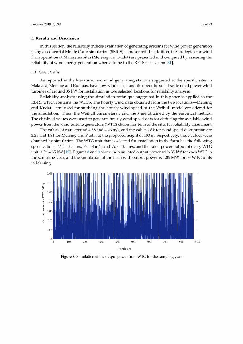
Processes 2019, 7, 399 17 of 23

5. Results and Discussion

In this section, the reliability indices evaluation of generating systems for wind power generationusing a sequential Monte Carlo simulation (SMCS) is presented. In addition, the strategies for windfarm operation at Malaysian sites (Mersing and Kudat) are presented and compared by assessing thereliability of wind energy generation when adding to the RBTS test system [31].

5.1. Case Studies

As reported in the literature, two wind generating stations suggested at the specific sites inMalaysia, Mersing and Kudatas, have low wind speed and thus require small-scale rated power windturbines of around 35 kW for installation in two selected locations for reliability analysis.

Reliability analysis using the simulation technique suggested in this paper is applied to theRBTS, which contains the WECS. The hourly wind data obtained from the two locations—Mersingand Kudat—atre used for studying the hourly wind speed of the Weibull model considered forthe simulation. Then, the Weibull parameters c and the k are obtained by the empirical method.The obtained values were used to generate hourly wind speed data for deducing the available windpower from the wind turbine generators (WTG) chosen for both of the sites for reliability assessment.

The values of c are around 4.88 and 4.46 m/s, and the values of k for wind speed distribution are2.25 and 1.84 for Mersing and Kudat at the proposed height of 100 m, respectively; these values wereobtained by simulation. The WTG unit that is selected for installation in the farm has the followingspecifications: Vci = 3.5 m/s, Vr = 8 m/s, and Vco = 25 m/s, and the rated power output of every WTGunit is Pr = 35 kW [19]. Figures 8 and 9 show the simulated output power with 35 kW for each WTG inthe sampling year, and the simulation of the farm with output power is 1.85 MW for 53 WTG unitsin Mersing.Processes 2019, 7, x FOR PEER REVIEW 19 of 26

Figure 8. Simulation of the output power from WTG for the sampling year.

Figure 9. Simulation of the output power from wind farm for the sampling year.

Figure 10. The available capacity of the generation system which is superimposed with the

chronologically available load model.


Processes 2019, 7, 399 18 of 23







The RBTS was simulated for 600 trials using the SMCS method. The simulation proceeded inchronological order from one hour to the next, repeatedly, using yearly samples until the specifiedconvergence criteria were met. Figure 10 shows the available capacity for the power system containingwind power generation from the wind farm in Mersing during the simulated process for yearlysamples and the superimposition of the available capacity with the chronological load model. It can beseen from this state of the system that the available capacity of the power generating system is notsufficient to meet the load demands. Thus, there are some intersections that are seen in the diagram.Figure 11 represents the reliability indices for simulation with (600) sampling years. The values ofLOLE, the amount of the LOEE, and the frequency of losing a load during the simulation process aredepicted in Figure 11 for wind power in the Mersing site.






Figure 10. The available capacity of the generation system which is superimposed with thechronologically available load model.

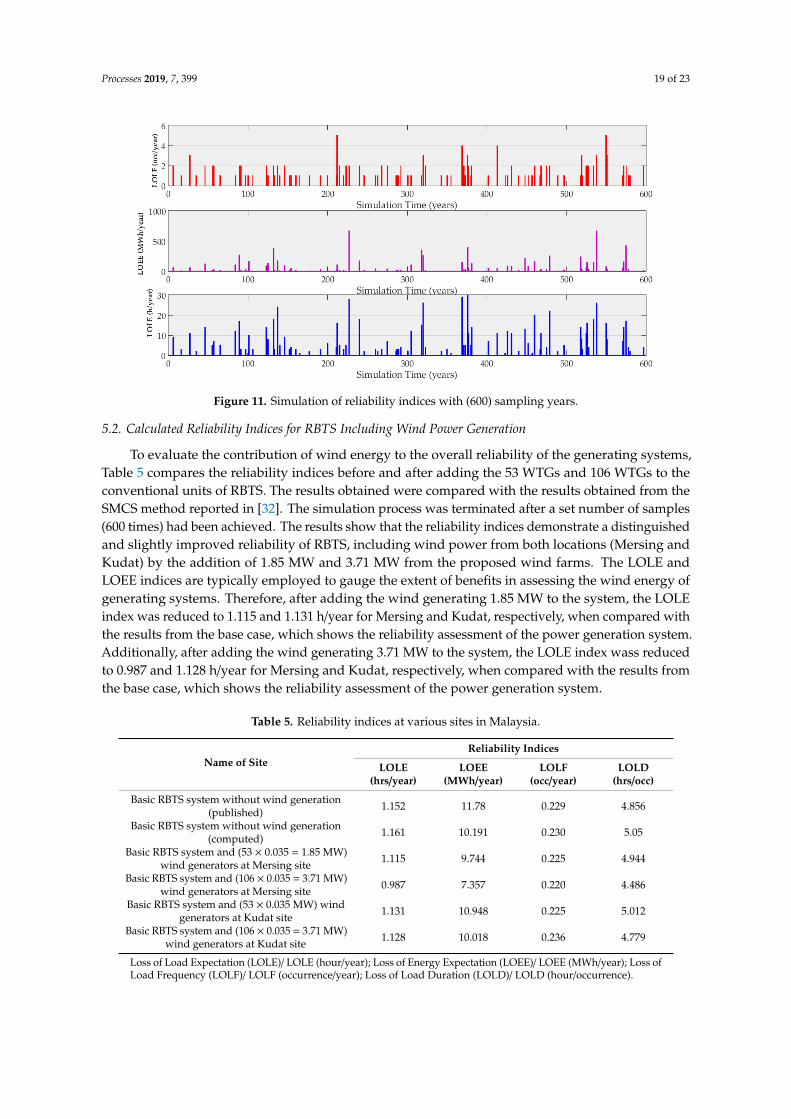
Processes 2019, 7, 399 19 of 23


Figure 11. Simulation of reliability indices with (600) sampling years.

5.2. Calculated Reliability Indices for RBTS Including Wind Power Generation

To evaluate the contribution of wind energy to the overall reliability of the generating systems,

Table 5 compares the reliability indices before and after adding the 53 WTGs and 106 WTGs to the

conventional units of RBTS. The results obtained were compared with the results obtained from the

SMCS method reported in [32]. The simulation process was terminated after a set number of samples

(600 times) had been achieved. The results show that the reliability indices demonstrate a

distinguished and slightly improved reliability of RBTS, including wind power from both locations

(Mersing and Kudat) by the addition of 1.85 MW and 3.71 MW from the proposed wind farms. The

LOLE and LOEE indices are typically employed to gauge the extent of benefits in assessing the wind

energy of generating systems. Therefore, after adding the wind generating 1.85 MW to the system,

the LOLE index was reduced to 1.115 and 1.131 h/year for Mersing and Kudat, respectively, when

compared with the results from the base case, which shows the reliability assessment of the power

generation system. Additionally, after adding the wind generating 3.71 MW to the system, the LOLE

index wass reduced to 0.987 and 1.128 h/year for Mersing and Kudat, respectively, when compared

with the results from the base case, which shows the reliability assessment of the power generation

system.

Figure 11. Simulation of reliability indices with (600) sampling years.

5.2. Calculated Reliability Indices for RBTS Including Wind Power Generation

To evaluate the contribution of wind energy to the overall reliability of the generating systems,Table 5 compares the reliability indices before and after adding the 53 WTGs and 106 WTGs to theconventional units of RBTS. The results obtained were compared with the results obtained from theSMCS method reported in [32]. The simulation process was terminated after a set number of samples(600 times) had been achieved. The results show that the reliability indices demonstrate a distinguishedand slightly improved reliability of RBTS, including wind power from both locations (Mersing andKudat) by the addition of 1.85 MW and 3.71 MW from the proposed wind farms. The LOLE andLOEE indices are typically employed to gauge the extent of benefits in assessing the wind energy ofgenerating systems. Therefore, after adding the wind generating 1.85 MW to the system, the LOLEindex was reduced to 1.115 and 1.131 h/year for Mersing and Kudat, respectively, when compared withthe results from the base case, which shows the reliability assessment of the power generation system.Additionally, after adding the wind generating 3.71 MW to the system, the LOLE index wass reducedto 0.987 and 1.128 h/year for Mersing and Kudat, respectively, when compared with the results fromthe base case, which shows the reliability assessment of the power generation system.

Table 5. Reliability indices at various sites in Malaysia.

Name of SiteReliability Indices

LOLE(hrs/year)

LOEE(MWh/year)

LOLF(occ/year)

LOLD(hrs/occ)

Basic RBTS system without wind generation(published) 1.152 11.78 0.229 4.856

Basic RBTS system without wind generation(computed) 1.161 10.191 0.230 5.05

Basic RBTS system and (53 × 0.035 = 1.85 MW)wind generators at Mersing site 1.115 9.744 0.225 4.944

Basic RBTS system and (106 × 0.035 = 3.71 MW)wind generators at Mersing site 0.987 7.357 0.220 4.486

Basic RBTS system and (53 × 0.035 MW) windgenerators at Kudat site 1.131 10.948 0.225 5.012

Basic RBTS system and (106 × 0.035 = 3.71 MW)wind generators at Kudat site 1.128 10.018 0.236 4.779

Loss of Load Expectation (LOLE)/ LOLE (hour/year); Loss of Energy Expectation (LOEE)/ LOEE (MWh/year); Loss ofLoad Frequency (LOLF)/ LOLF (occurrence/year); Loss of Load Duration (LOLD)/ LOLD (hour/occurrence).

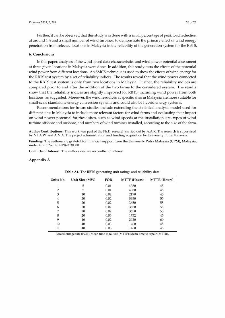
Processes 2019, 7, 399 20 of 23

Further, it can be observed that this study was done with a small percentage of peak load reductionat around 1% and a small number of wind turbines, to demonstrate the primary effect of wind energypenetration from selected locations in Malaysia in the reliability of the generation system for the RBTS.

6. Conclusions

In this paper, analyses of the wind speed data characteristics and wind power potential assessmentat three given locations in Malaysia were done. In addition, this study tests the effects of the potentialwind power from different locations. An SMCS technique is used to show the effects of wind energy forthe RBTS test system by a set of reliability indices. The results reveal that the wind power connectedto the RBTS test system is only from two locations in Malaysia. Further, the reliability indices arecompared prior to and after the addition of the two farms to the considered system. The resultsshow that the reliability indices are slightly improved for RBTS, including wind power from bothlocations, as suggested. Moreover, the wind resources at specific sites in Malaysia are more suitable forsmall-scale standalone energy conversion systems and could also be hybrid energy systems.

Recommendations for future studies include extending the statistical analysis model used fordifferent sites in Malaysia to include more relevant factors for wind farms and evaluating their impacton wind power potential for these sites, such as wind speeds at the installation site, types of windturbine offshore and onshore, and numbers of wind turbines installed, according to the size of the farm.

Author Contributions: This work was part of the Ph.D. research carried out by A.A.K. The research is supervisedby N.I.A.W. and A.N.A. The project administration and funding acquisition by University Putra Malaysia.

Funding: The authors are grateful for financial support from the University Putra Malaysia (UPM), Malaysia,under Grant No. GP-IPB-9630000.

Conflicts of Interest: The authors declare no conflict of interest.

Appendix A

Table A1. The RBTS generating unit ratings and reliability data.

Units No. Unit Size (MW) FOR MTTF (Hours) MTTR (Hours)

1 5 0.01 4380 452 5 0.01 4380 453 10 0.02 2190 454 20 0.02 3650 555 20 0.02 3650 556 20 0.02 3650 557 20 0.02 3650 558 20 0.03 1752 459 40 0.02 2920 60

10 40 0.03 1460 4511 40 0.03 1460 45

Forced outage rate (FOR); Mean time to failure (MTTF); Mean time to repair (MTTR).

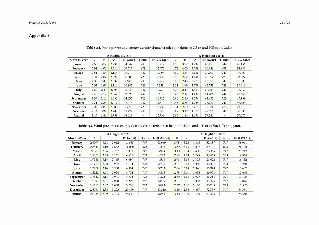
Processes 2019, 7, 399 21 of 23

Appendix B

Table A2. Wind power and energy density characteristics at heights of 3.5 m and 100 m in Kudat.


Appendix B

Table B1. Wind power and energy density characteristics at heights of 3.5 m and 100 m in Kudat.






Annual 2.45 1.84 2.759 18.819 - 13.738 3.95 1.84 4.456 79.284 - 57.877

Table A3. Wind power and energy density characteristics at height of 5.2 m and 100 m in Kuala Terengganu.


Table B2. Wind power and energy density characteristics at height of 5.2 m and 100 m in Kuala Terengganu.






Annual 2.0338 2.09 2.293 9.390 - 6.854 3.10 2.09 3.499 33.366 - 24.356

Processes 2019, 7, 399 22 of 23

References

1. Ouammi, A.; Dagdougui, H.; Sacile, R.; Mimet, A. Monthly and seasonal of wind energy characteristicsat four monitored locationals in Liguria region (Italy). Renew. Sustain. Energy Rev. 2010, 14, 1959–1968.[CrossRef]

2. Chaiamarit, K.; Nuchprayoon, S. Modeling of renewable energy resources for generation reliability evaluation.Renew. Sustain. Energy Rev. 2013, 26, 34–41. [CrossRef]

3. Shi, S.; Lo, K.L. An Overview of Wind Energy Development and Associated Power System ReliabilityEvaluation Methods. In Proceedings of the 2013 48th International Universities Power Engineering Conference(UPEC), Dublin, Ireland, 2–5 September 2013; pp. 1–6.

4. Benidris, M.; Mitra, J. Composite Power System Reliability Assessment Using Maximum Capacity Flow andDirected Binary Particle Swarm Optimization. In Proceedings of the IEEE Conference, Manhattan, KS, USA,22–24 September 2013; pp. 1–6.

5. Padma, L.M.; Harshavardham, R.P.; Janardhana, N.P. Generation Reliability Evaluation of Wind EnergyPenetrated Power System. In Proceedings of the International Conference on High Performance Computingand Applications (ICHPCA), Odisha, India, 22–24 December 2014; pp. 1–4.

6. Islam, M.R.; Saidur, R.; Rahim, N.A. Assessment of wind energy potentiality at Kudat and Labuan,Malaysia using Weibull distribution function. Energy 2011, 36, 985–992. [CrossRef]

7. Taylor, P.; Khatib, T.; Sopian, K.; Ibrahim, M.Z. Assessment of electricity generation by wind power in ninecostal sites in Malaysia. Int. J. Ambient Energy 2013, 37–41. [CrossRef]

8. Gebrelibanos, K.G. Feasibility Study of Small Scale Standalone Wind Turbine for Urban Area: Case Study: KTHMain Campus; KTH School of Industrial Engineering and Management, Energy Technology EGI: Stockholm,Sweden, 2013.

9. Siti, M.R.S.; Norizah, M.; Syafrudin, M. The Evaluation of Wind Energy Potential in Peninsular Malaysia.Int. J. Chem. Environ. Eng. 2011, 2, 284–291.

10. Kadhem, A.A.; Abdul, W.N.I.; Aris, I.; Jasni, J.; Abdalla, A.N. Advanced Wind Speed Prediction Model Basedon Combination of Weibull Distribution and Artificial Neural Network. Energies 2017, 10, 1744. [CrossRef]

11. Borhanazad, H.; Mekhilef, S.; Saidur, R.; Boroumandjazi, G. Potential application of renewable energy forrural electrification in Malaysia. Renew. Energy 2013, 59, 210–219. [CrossRef]

12. Irwanto, M.; Gomesh, N.; Mamat, M.R.; Yusoff, Y.M. Assessment of wind power generation potential inPerlis, Malaysia. Renew. Sustain. Energy Rev. 2014, 38, 296–308. [CrossRef]

13. Albani, A.; Ibrahim, M.Z.; Yong, K.H. Wind Energy Investigation in Northern Part of Kudat, Malaysia. Int. J.Eng. Appl. Sci. 2013, 2, 14–22.

14. Goh, H.H.; Lee, S.W.; Chua, Q.S.; Teo, K.T.K. Wind energy assessment considering wind speed correlation inMalaysia. Renew. Sustain. Energy Rev. 2016, 54, 1389–1400. [CrossRef]

15. Hwang, G.H.; Lin, N.S.; Ching, K.B.; Wei, L.S. Wind Farm Allocation In Malaysia Based On Multi-CriteriaDecision Making Method. In Proceedings of the National Postgraduate Conference (NPC), Seri Iskandar,Malaysia, 19–20 September 2011; pp. 1–6.

16. Chang, T.P. Performance comparison of six numerical methods in estimating Weibull parameters for windenergy application. Appl. Energy 2011, 88, 272–282. [CrossRef]

17. Kaoga, D.K.; Serge, D.Y.; Raidandi, D.; Djongyang, N. Performance Assessment of Two-parameter WeibullDistribution Methods for Wind Energy Applications in the District of Maroua in Cameroon. Int. J. Sci. BasicAppl. Res. 2014, 17, 39–59.

18. Kidmo, D.K.; Danwe, R.; Doka, S.Y.; Djongyang, N. Statistical analysis of wind speed distribution based onsix Weibull Methods for wind power evaluation in Garoua, Cameroon. Rev. Des. Energ. Renouv. 2015, 18,105–125.

19. Adaramola, M.S.; Oyewola, O.M.; Ohunakin, O.S.; Akinnawonu, O.O. Performance evaluation of windturbines for energy generation in Niger. Sustain. Energy Technol. Assess. 2014, 6, 75–85. [CrossRef]

20. Ohunakin, O.S.; Adaramola, M.S.; Oyewola, O.M. Wind energy evaluation for electricity generation usingWECS in seven selected locations in Nigeria. Appl. Energy 2011, 88, 3197–3206. [CrossRef]

21. Oyedepo, S.O.; Adaramola, M.S.; Paul, S.S. Analysis of wind speed data and wind energy potential in threeselected locations in south-east Nigeria. Int. J. Energy Environ. Eng. 2012, 3, 1–11. [CrossRef]

http://dx.doi.org/10.1016/j.rser.2010.04.015


http://dx.doi.org/10.1016/j.energy.2010.12.011

http://dx.doi.org/10.1080/01430750.2012.740428

http://dx.doi.org/10.3390/en10111744

http://dx.doi.org/10.1016/j.renene.2013.03.039



http://dx.doi.org/10.1016/j.apenergy.2010.06.018

http://dx.doi.org/10.1016/j.seta.2014.01.001

http://dx.doi.org/10.1016/j.apenergy.2011.03.022

http://dx.doi.org/10.1186/2251-6832-3-7

Processes 2019, 7, 399 23 of 23

22. Anurag, C.; Saini, R.P. Statistical Analysis of Wind Speed Data Using Weibull Distribution Parameters.In Proceedings of the 1st International Conference on Non-Conventional Energy (ICONCE 2014), Kalyani,India, 16–17 January 2014; pp. 160–163.

23. Molina-García, A.; Fernández-Guillamón, A.; Gómez-Lázaro, E.; Honrubia-Escribano, A.; Bueso, M.C.Vertical Wind Profile Characterization and Identification of Patterns Based on a Shape Clustering Algorithm; IEEE:New York, NY, USA, 2019; Volume 7, pp. 30890–30904.

24. Ahmed, A.S. Wind energy as a potential generation source at Ras Benas, Egypt. Renew. Sustain. Energy Rev.2010, 14, 2167–2173. [CrossRef]

25. Hussain, M.Z.; Roy, D.K.; Khan, S.; Sharma, P.K.; Talukdar, R. Wind Energy Potential at Different Cities ofAssam Using Statistical Models. Int. J. Adv. Res. Innov. 2018, 6, 38–43.

26. Ayodele, T.R.; Ogunjuyigbe, A.S.O.; Amusan, T.O. Wind power utilization assessment and economic analysisof wind turbines across fifteen locations in the six geographical zones of Nigeria. J. Clean. Prod. 2016, 129,341–349. [CrossRef]

27. Chandel, S.S.; Ramasamy, P.; Murthy, K.S.R. Wind power potential assessment of 12 locations in westernHimalayan region of India. Renew. Sustain. Energy Rev. 2014, 39, 530–545. [CrossRef]

28. Shi, S. Operation and Assessment of Wind Energy on Power System Reliability Evaluation. Ph.D. Thesis,Department of Electronic and Electrical Engineering, University of Strathclyde, Glasgow, Scotland, 2014.

29. Dursun, B.; Alboyaci, B. An Evaluation of Wind Energy Characteristics for Four Different Locations inBalikesir. Energy Sour. Part A: Recovery Util. Environ. Eff. 2011, 33, 1086–1103. [CrossRef]

30. Ayodele, T.R.; Jimoh, A.A.; Munda, J.L.; AgeeWind, J.T. distribution and capacity factor estimation for windturbines in the coastal region of South Africa. Energy Convers Manag. 2012, 64, 614–625. [CrossRef]

31. Heshmati, A.; Najafi, H.R.; Aghaebrahimi, M.R.; Mehdizadeh, M. Wind Farm Modeling For ReliabilityAssessment from the Viewpoint of Interconnected Systems. Electr. Power Compon. Syst. 2012, 40, 257–272.[CrossRef]

32. Kadhem, A.A.; Abdul Wahab, N.I.; Aris, I.; Jasni, J.; Abdalla, A.N. Computational techniques for assessingthe reliability and sustainability of electrical power systems: A review. Renew. Sustain. Energy Rev. 2017, 80,1175–1186. [CrossRef]

© 2019 by the authors. Licensee MDPI, Basel, Switzerland. This article is an open accessarticle distributed under the terms and conditions of the Creative Commons Attribution(CC BY) license (http://creativecommons.org/licenses/by/4.0/).


http://dx.doi.org/10.1016/j.jclepro.2016.04.060


http://dx.doi.org/10.1080/15567030903330850

http://dx.doi.org/10.1016/j.enconman.2012.06.007

http://dx.doi.org/10.1080/15325008.2011.631086


http://creativecommons.org/

http://creativecommons.org/licenses/by/4.0/.

wind energy generation assessment at speciﬁc sites in a

Documents