with de boer, haehl, heller & neiman arxiv:1509.00113; … · 2017-09-26 · with de boer,...
TRANSCRIPT

with de Boer, Haehl, Heller & Neiman arXiv:1509.00113; arXiv:1605.nnnnn
•TexPoint fonts used in EMF. •Read the TexPoint manual before you delete this box.: AAAAAA

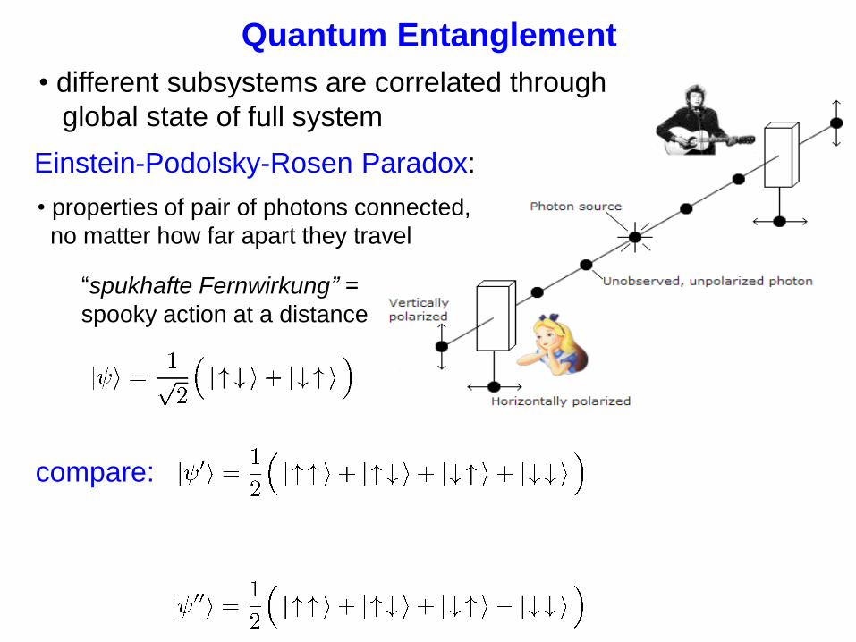
Quantum Entanglement
“spukhafte Fernwirkung” =
spooky action at a distance
Einstein-Podolsky-Rosen Paradox:
• properties of pair of photons connected,
no matter how far apart they travel
• different subsystems are correlated through
global state of full system
Quantum Entanglement
“spukhafte Fernwirkung” =
spooky action at a distance
Einstein-Podolsky-Rosen Paradox:
• properties of pair of photons connected,
no matter how far apart they travel
• different subsystems are correlated through
global state of full system
compare:

Quantum Entanglement
“spukhafte Fernwirkung” =
spooky action at a distance
Einstein-Podolsky-Rosen Paradox:
• properties of pair of photons connected,
no matter how far apart they travel
• different subsystems are correlated through
global state of full system
compare:
Entangled!!
No Entanglement!!

Entanglement Entropy
• in QFT, typically introduce a (smooth) boundary or entangling
surface which divides the space into two separate regions
• integrate out degrees of freedom in “outside” region
• remaining dof are described by a density matrix
A
B
calculate von Neumann entropy:
• general tool; divide quantum system into two parts and use
entropy as measure of correlations between subsystems

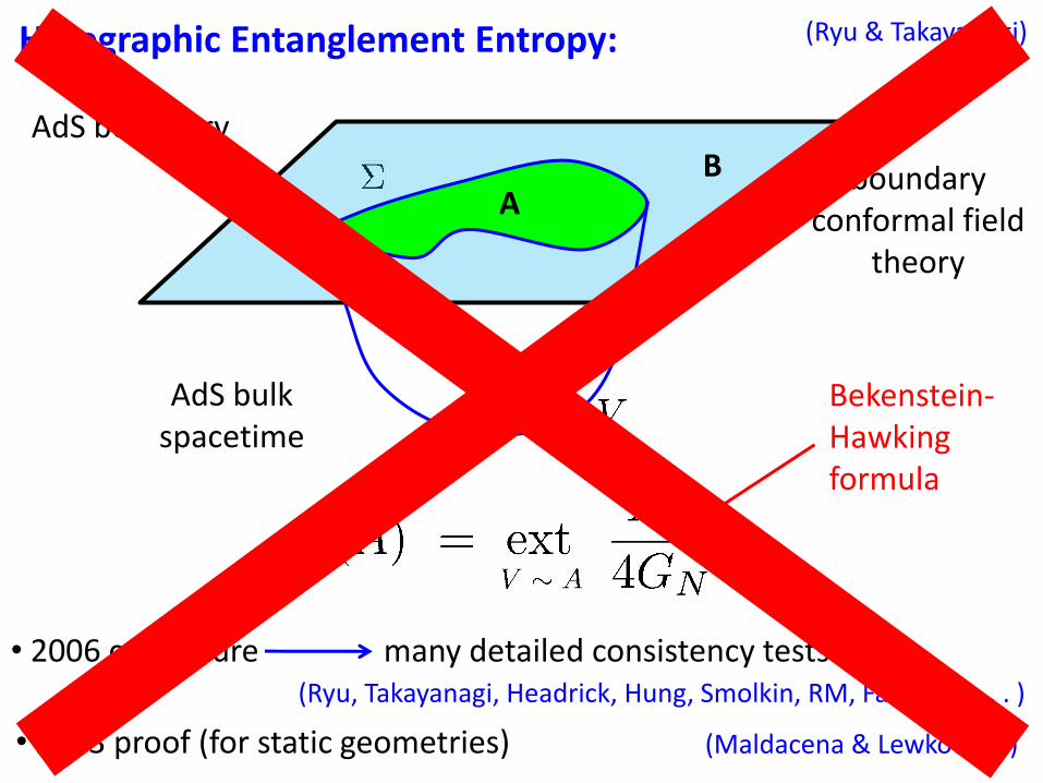
Holographic Entanglement Entropy: (Ryu & Takayanagi)
A B
AdS boundary
AdS bulk spacetime
boundary conformal field
theory
Bekenstein- Hawking formula
• 2006 conjecture many detailed consistency tests (Ryu, Takayanagi, Headrick, Hung, Smolkin, RM, Faulkner, . . . )
(Maldacena & Lewkowycz) • 2013 proof (for static geometries)

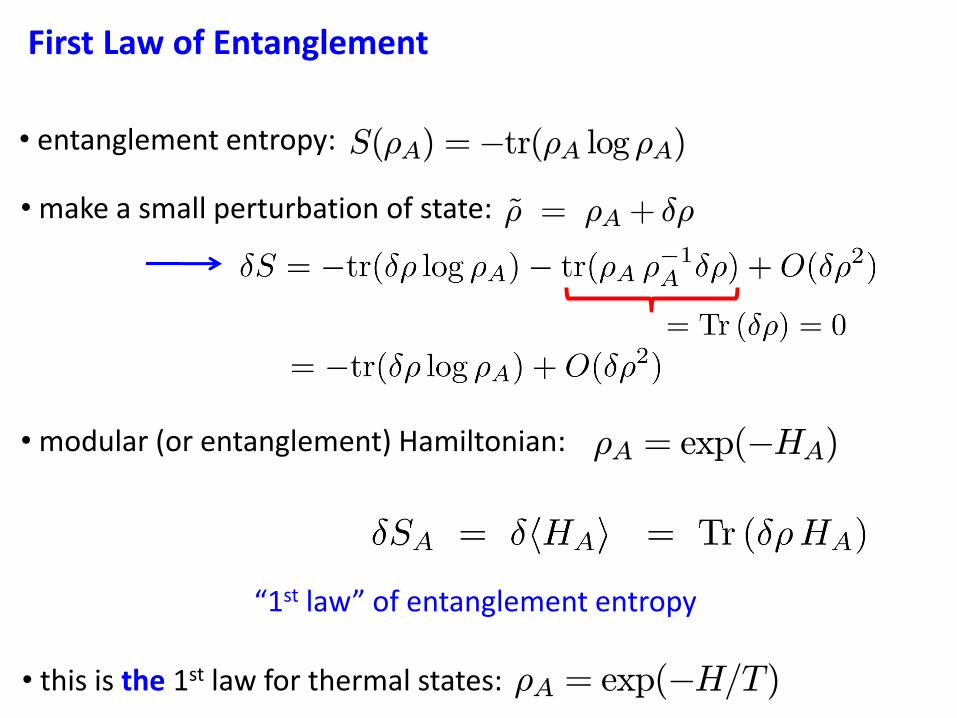
First Law of Entanglement
• entanglement entropy:
• make a small perturbation of state:
S(½A) =¡tr(½A log½A)
~½ = ½A+ ±½

First Law of Entanglement
• entanglement entropy:
• make a small perturbation of state:
S(½A) =¡tr(½A log½A)
~½ = ½A+ ±½
“1st law” of entanglement entropy
½A = exp(¡HA)• modular (or entanglement) Hamiltonian:
First Law of Entanglement
• entanglement entropy:
• make a small perturbation of state:
S(½A) =¡tr(½A log½A)
~½ = ½A+ ±½
“1st law” of entanglement entropy
½A = exp(¡HA)• modular (or entanglement) Hamiltonian:
½A = exp(¡H=T)• this is the 1st law for thermal states:

“1st law” of entanglement entropy:
• generally is “nonlocal mess” and flow is nonlocal/not geometric
HA =
Zdd¡1x°¹º1 (x)T¹º +
Zdd¡1x
Zdd¡1y °¹º;½¾2 (x; y)T¹ºT½¾ + ¢ ¢ ¢
hence usefulness of first law is very limited, in general

“1st law” of entanglement entropy:
• generally is “nonlocal mess” and flow is nonlocal/not geometric
HA =
Zdd¡1x°¹º1 (x)T¹º +
Zdd¡1x
Zdd¡1y °¹º;½¾2 (x; y)T¹ºT½¾ + ¢ ¢ ¢
hence usefulness of first law is very limited, in general
• famous exception: Rindler wedge
HA = 2¼K
= 2¼
Z
A(x>0)
dd¡2y dx [x Ttt ] + c0
boost generator
A B ● Σ
Σ = (x = 0, t = 0) • any QFT in Minkowski vacuum; choose

• by causality, and describe physics throughout domain of dependence ; eg, generate boost flows
“1st law” of entanglement entropy:
• generally is “nonlocal mess” and flow is nonlocal/not geometric
HA =
Zdd¡1x°¹º1 (x)T¹º +
Zdd¡1x
Zdd¡1y °¹º;½¾2 (x; y)T¹ºT½¾ + ¢ ¢ ¢
hence usefulness of first law is very limited, in general
• famous exception: Rindler wedge
HA = 2¼K
= 2¼
Z
A(x>0)
dd¡2y dx [x Ttt ] + c0
boost generator
A B ●
HA
Σ
Σ = (x = 0, t = 0) • any QFT in Minkowski vacuum; choose
(Bisognano & Wichmann; Unruh)

• another exception: CFT in vacuum of d-dim. flat space and entangling surface which is Sd-2 with radius R
HB = 2¼
Z
B
dd¡1yR2 ¡ j~yj2
2RTtt(~y) + c0
(Casini, Huerta & RM; Hislop & Longo)
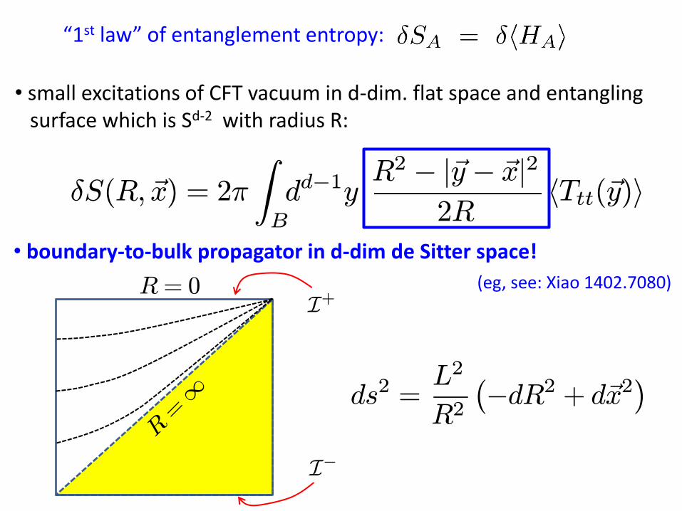
“1st law” of entanglement entropy:
B
B

“1st law” of entanglement entropy:
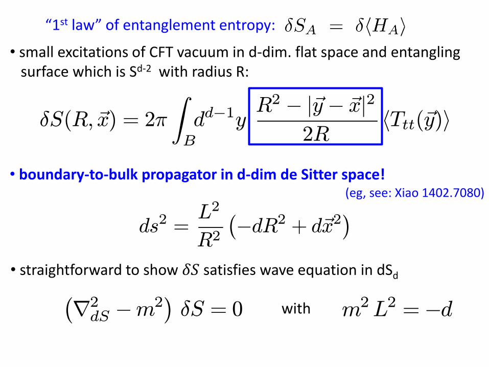
• small excitations of CFT vacuum in d-dim. flat space and entangling surface which is Sd-2 with radius R:
B
B
±S = ±hHBi = 2¼
Z
B
dd¡1yR2 ¡ j~yj2
2RhTtt(~y)i

±S(R;~x) = 2¼
Z
B
dd¡1yR2 ¡ j~y¡ ~xj2
2RhTtt(~y)i
“1st law” of entanglement entropy:
• small excitations of CFT vacuum in d-dim. flat space and entangling surface which is Sd-2 with radius R:
B
B R ●
𝑥
±S(R;~x) = 2¼
Z
B
dd¡1yR2 ¡ j~y¡ ~xj2
2RhTtt(~y)i
• boundary-to-bulk propagator in d-dim de Sitter space!
(eg, see: Xiao 1402.7080)
ds2 =L2
R2
¡¡dR2 + d~x2
¢
R=1
I+
I¡
R= 0
“1st law” of entanglement entropy:
• small excitations of CFT vacuum in d-dim. flat space and entangling surface which is Sd-2 with radius R:
• small excitations of CFT vacuum in d-dim. flat space and entangling surface which is Sd-2 with radius R:
±S(R;~x) = 2¼
Z
B
dd¡1yR2 ¡ j~y¡ ~xj2
2RhTtt(~y)i
• boundary-to-bulk propagator in d-dim de Sitter space! (eg, see: Xiao 1402.7080)
ds2 =L2
R2
¡¡dR2 + d~x2
¢
• straightforward to show 𝛿𝑆 satisfies wave equation in dSd
¡r2dS ¡m2
¢±S = 0 m2L2 =¡dwith
“1st law” of entanglement entropy:
• wave equation is singular as 𝑅 → 0
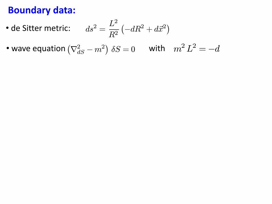
Boundary data:
ds2 =L2
R2
¡¡dR2 + d~x2
¢
¡r2dS ¡m2
¢±S = 0
• de Sitter metric:
with m2L2 =¡d

• wave equation is singular as 𝑅 → 0
Boundary data:
ds2 =L2
R2
¡¡dR2 + d~x2
¢
¡r2dS ¡m2
¢±S = 0
• de Sitter metric:
±SR!0= F(~x)=R+ f(~x)Rd + ¢ ¢ ¢2 independent sol’s:
¢= d¢=¡1

• wave equation is singular as 𝑅 → 0
Boundary data:
ds2 =L2
R2
¡¡dR2 + d~x2
¢
¡r2dS ¡m2
¢±S = 0
• de Sitter metric:
±SR!0= F(~x)=R+ f(~x)Rd + ¢ ¢ ¢2 independent sol’s:
• “1st law” solution:
f(~x) =¼d+12
¡¡d+32
¢ hTtt(~x)i
¢= d¢=¡1
F(~x) = 0 ;
±S(R;~x) = 2¼
Z
B
dd¡1yR2 ¡ j~y¡ ~xj2
2RhTtt(~y)i

• sets 𝛿𝑆 at very small 𝑅 and EE perturbations at larger scales determined by the local Lorentzian propagation into dS geometry
• wave equation is singular as 𝑅 → 0
Boundary data:
ds2 =L2
R2
¡¡dR2 + d~x2
¢
¡r2dS ¡m2
¢±S = 0
• de Sitter metric:
±SR!0= F(~x)=R+ f(~x)Rd + ¢ ¢ ¢2 independent sol’s:
• “1st law” solution:
f(~x) =¼d+12
¡¡d+32
¢ hTtt(~x)i
¢= d¢=¡1
F(~x) = 0 ;
hTtti
±S(R;~x) = 2¼
Z
B
dd¡1yR2 ¡ j~y¡ ~xj2
2RhTtt(~y)i

• : mass tachyonic! → above precisely removes the “non-normalizable” or unstable modes
• sets 𝛿𝑆 at very small 𝑅 and EE perturbations at larger scales determined by the local Lorentzian propagation into dS geometry
• wave equation is singular as 𝑅 → 0
Boundary data:
ds2 =L2
R2
¡¡dR2 + d~x2
¢
¡r2dS ¡m2
¢±S = 0
m2L2 =¡d
• de Sitter metric:
±SR!0= F(~x)=R+ f(~x)Rd + ¢ ¢ ¢2 independent sol’s:
• “1st law” solution:
f(~x) =¼d+12
¡¡d+32
¢ hTtt(~x)i
¢= d¢=¡1
F(~x) = 0 ;
hTtti
±S(R;~x) = 2¼
Z
B
dd¡1yR2 ¡ j~y¡ ~xj2
2RhTtt(~y)i

Example: ±S(R;~x) = 2¼
Z
B
dd¡1yR2 ¡ j~y¡ ~xj2
2RhTtt(~y)i
• consider state: jÃi = j0i + ² Ttt(t0 + i¿; ~x0)j0iregulate UV divergences
small expansion parameter
²=¿d ¿ 1

Example: ±S(R;~x) = 2¼
Z
B
dd¡1yR2 ¡ j~y¡ ~xj2
2RhTtt(~y)i
• consider state: jÃi = j0i + ² Ttt(t0 + i¿; ~x0)j0iregulate UV divergences
small expansion parameter
²=¿d ¿ 1
• expectation value is fixed by 2-pt function
hÃjTtt(t; x)jÃi = ² CT
"1
(¢x2 ¡ (¢t+ i ¿)2)d
Ã(¢x2 + (¢t+ i ¿)2)2
(¢x2 ¡ (¢t+ i ¿)2)2¡1
d
!+c:c:
#
+ O(²2)
h0jTtt(t; ~x)Ttt(0;~0)j0i
with and

Example: ±S(R;~x) = 2¼
Z
B
dd¡1yR2 ¡ j~y¡ ~xj2
2RhTtt(~y)i
• consider state: jÃi = j0i + ² Ttt(t0 + i¿; ~x0)j0iregulate UV divergences
small expansion parameter
²=¿d ¿ 1
d = 3: 𝑡 = 5, 𝑦 = 𝑦0
• sphere expanding out from (𝑡0, 𝑥 0) at speed of light

Example: ±S(R;~x) = 2¼
Z
B
dd¡1yR2 ¡ j~y¡ ~xj2
2RhTtt(~y)i
• consider state: jÃi = j0i + ² Ttt(t0 + i¿; ~x0)j0iregulate UV divergences
small expansion parameter
²=¿d ¿ 1
d = 3: 𝑡 = 5, 𝑦 = 𝑦0

Alternate conformal frames:
• wave equation is covariant ¡r2dS ¡m2
¢±S = 0
can use any coordinate system on dS geometry
• coord transformation in bulk corresponds to conformal transformation in boundary theory new holographic construction extends to CFT in any conformally flat background

Alternate conformal frames:
• wave equation is covariant ¡r2dS ¡m2
¢±S = 0
can use any coordinate system on dS geometry
ds2 = L2(¡d¿2 +cosh(¿)2dd¡1)
• coord transformation in bulk corresponds to conformal transformation in boundary theory new holographic construction extends to CFT in any conformally flat background
CFT time slice is 𝑆𝑑−1, in cylindrical bkgd 𝑅 × 𝑆𝑑−1
asymptotic boundary ( ) is round 𝑆𝑑−1
• for example, consider same wave equation in global dS coord’s
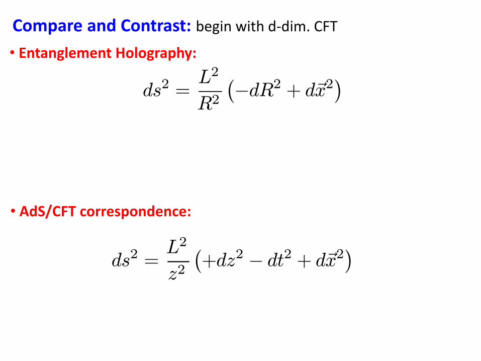
Compare and Contrast: begin with d-dim. CFT
ds2 =L2
R2
¡¡dR2 + d~x2
¢• Entanglement Holography:
• AdS/CFT correspondence:
ds2 =L2
z2
¡+dz2 ¡ dt2 + d~x2
¢

Compare and Contrast: begin with d-dim. CFT
ds2 =L2
R2
¡¡dR2 + d~x2
¢• Entanglement Holography:
• AdS/CFT correspondence:
ds2 =L2
z2
¡+dz2 ¡ dt2 + d~x2
¢
spatial coordinates in (d–1)-dim. time slice
spacetime coordinates for d-dim. CFT
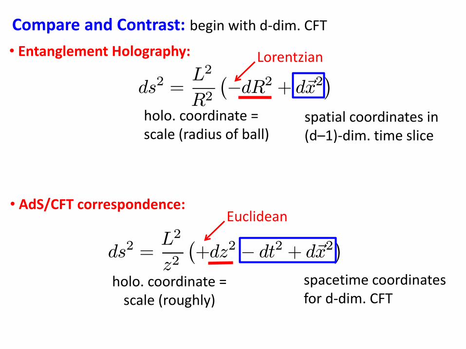
Compare and Contrast: begin with d-dim. CFT
ds2 =L2
R2
¡¡dR2 + d~x2
¢• Entanglement Holography:
• AdS/CFT correspondence:
ds2 =L2
z2
¡+dz2 ¡ dt2 + d~x2
¢
spatial coordinates in (d–1)-dim. time slice
spacetime coordinates for d-dim. CFT
holo. coordinate = scale (radius of ball)
holo. coordinate = scale (roughly)
Lorentzian
Euclidean

Compare and Contrast: begin with d-dim. CFT
ds2 =L2
R2
¡¡dR2 + d~x2
¢• Entanglement Holography:
• AdS/CFT correspondence:
ds2 =L2
z2
¡+dz2 ¡ dt2 + d~x2
¢
spatial coordinates in (d–1)-dim. time slice
spacetime coordinates for d-dim. CFT
holo. coordinate = scale (radius of ball)
holo. coordinate = scale (roughly)
• two-derivative wave equation relies only on first law of entanglement appropriate states in any CFT in any number of dimensions
Lorentzian
Euclidean
• two-derivative bulk theory relies on weak curvature and weak coupling holographic CFT requires strong coupling and large # of d.o.f.
undetermined constant?
fixed by ℓP

Compare and Contrast: begin with d-dim. CFT
ds2 =L2
R2
¡¡dR2 + d~x2
¢• Entanglement Holography:
• AdS/CFT correspondence:
ds2 =L2
z2
¡+dz2 ¡ dt2 + d~x2
¢
spatial coordinates in (d–1)-dim. time slice
spacetime coordinates for d-dim. CFT
holo. coordinate = scale (radius of ball)
holo. coordinate = scale (roughly)
• two-derivative wave equation relies only on first law of entanglement appropriate states in any CFT in any number of dimensions
Euclidean
• two-derivative bulk theory relies on weak curvature and weak coupling holographic CFT requires strong coupling and large # of d.o.f.
undetermined constant?
fixed by ℓP
Lorentzian

• geometry naturally gives partial ordering of spheres
time slice reference sphere
(ordering of intervals for d=2 discussed by Czech, Lamprou, McCandlish & Sully)
Why is scale time-like?

• geometry naturally gives partial ordering of spheres
time-like separated
time slice reference sphere
(ordering of intervals for d=2 discussed by Czech, Lamprou, McCandlish & Sully)
Why is scale time-like?

• geometry naturally gives partial ordering of spheres
time-like separated
time slice
space-like separated
reference sphere
(ordering of intervals for d=2 discussed by Czech, Lamprou, McCandlish & Sully)
Why is scale time-like?

• geometry naturally gives partial ordering of spheres
time-like separated
time slice
space-like separated
null separated
reference sphere
suggests auxiliary/holographic geometry should be Lorentzian
(ordering of intervals for d=2 discussed by Czech, Lamprou, McCandlish & Sully)
Why is scale time-like?

x
Bx
•
@Bx Bx
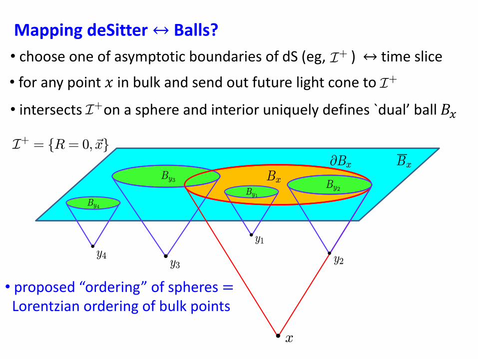
Mapping deSitter ↔ Balls?
• choose one of asymptotic boundaries of dS (eg, ) ↔ time slice I+
• for any point 𝑥 in bulk and send out future light cone to I+
• intersects on a sphere and interior uniquely defines `dual’ ball 𝐵𝑥 I+
I+ = fR = 0; ~xg
dS bulk
•
•
Bx
•
• • y4
y3 y2
By4
@Bx Bx
By2
By3
y1
By1
• choose one of asymptotic boundaries of dS (eg, ) ↔ time slice I+Mapping deSitter ↔ Balls?
I+ = fR = 0; ~xg
x
• proposed “ordering” of spheres = Lorentzian ordering of bulk points
• for any point 𝑥 in bulk and send out future light cone to I+
• intersects on a sphere and interior uniquely defines `dual’ ball 𝐵𝑥 I+

•
•
Bx
•
• • y4
y3 y2
By4
@Bx Bx
By2
By3
y1
By1
• choose one of asymptotic boundaries of dS (eg, ) ↔ time slice I+Mapping deSitter ↔ Balls?
I+ = fR = 0; ~xg
x
• proposed “ordering” of spheres = Lorentzian ordering of bulk points
• mapping/dS geometry does not imply local dynamics respecting this structure
• for any point 𝑥 in bulk and send out future light cone to I+
• intersects on a sphere and interior uniquely defines `dual’ ball 𝐵𝑥 I+

Comments:
• same wave equation derived from AdS/CFT correspondence
Nozaki, Numasawa, Prudenziati& Takayanagi: arXiv:1304.7100 Bhattacharya, Takayanagi: arXiv:1308.3792
• Eg, linearized Einstein eqs in AdS4 implied for holographic EE ·@2
@R2¡ 1
R
@
@R¡ 3
R2¡ @2
@x2¡ @2
@y2
¸±S(t; x; y;R) = 0
• here, we see equation readily extends to any 𝑑 and follows purely from underlying conformal symmetry
·¡R3
L2
@
@R
µ1
R
@
@R
¶+R2
L2
@2
@x2+R2
L2
@2
@y2+
3
L2
¸±S(t; x; y;R) = 0
• can be recast as d=3 deSitter wave equation:
mass term d’Alembertian on dS3
Comments:
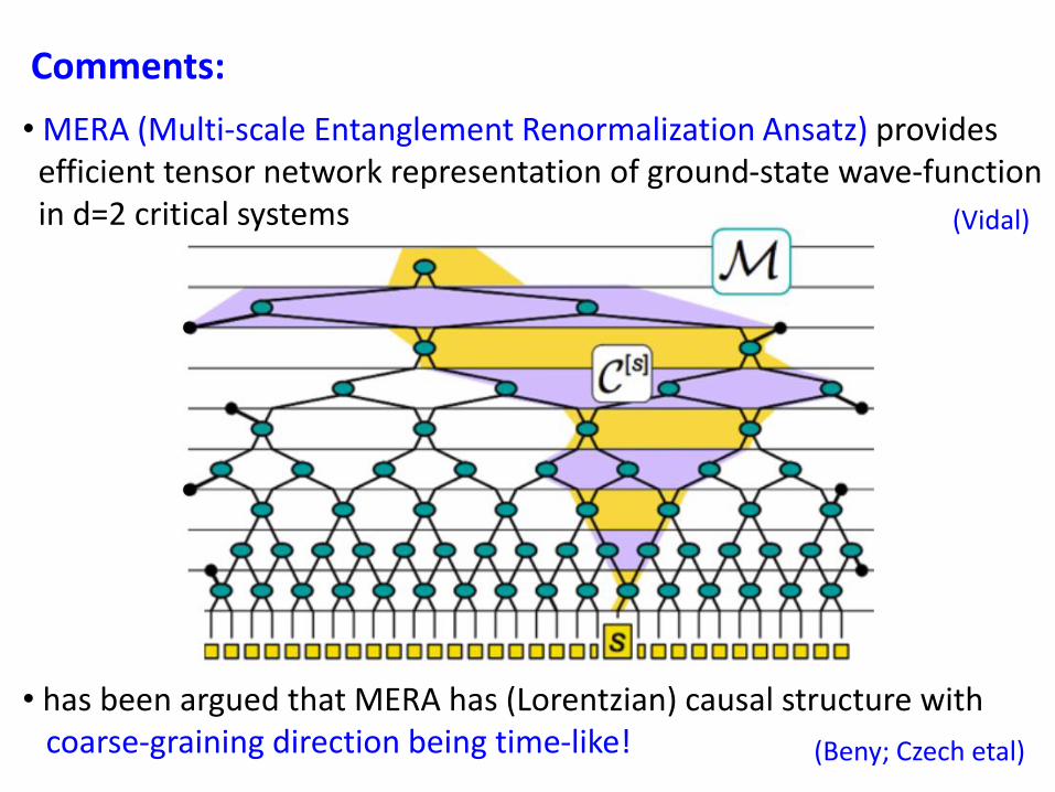
• MERA (Multi-scale Entanglement Renormalization Ansatz) provides efficient tensor network representation of ground-state wave-function in d=2 critical systems (Vidal)
• has been argued that MERA has (Lorentzian) causal structure with coarse-graining direction being time-like! (Beny; Czech etal)

Comments:
• deSitter geometry appears in recent discussions of integral geometry and the interpretation of MERA in terms of AdS3/CFT2
(Czech, Lamprou, McCandlish & Sully: arXiv:1505.05515; arXiv:1512.01548)
• consider space of intervals u<x<v on time slice of 2d holographic CFT space of geodesics on 2d slice of AdS3 pts in 2d de Sitter AdS/CFT
ds2 = L2 dudv
(v ¡ u)2
dS scale?
motivate the choice: L2 =c
3
ds2 = @u@vS0 dudv
with S0 =c
3log
v ¡ u
±
volume in dS2 = length in AdS3 slice
“hole-ography”:
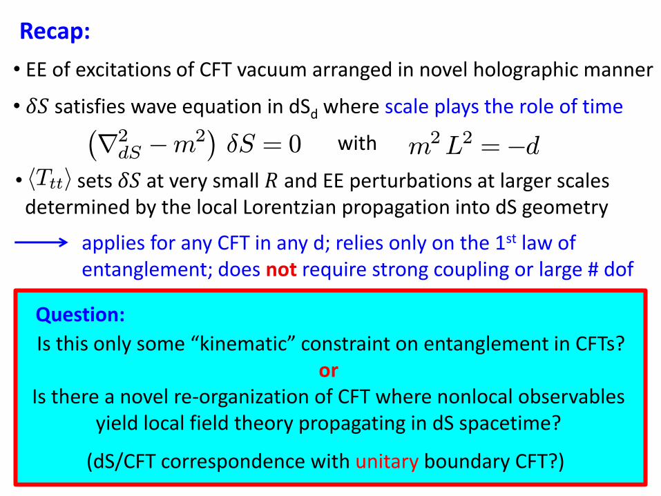
Recap:
• 𝛿𝑆 satisfies wave equation in dSd where scale plays the role of time ¡r2dS ¡m2
¢±S = 0 m2L2 =¡dwith
• sets 𝛿𝑆 at very small 𝑅 and EE perturbations at larger scales determined by the local Lorentzian propagation into dS geometry
hTtti
• EE of excitations of CFT vacuum arranged in novel holographic manner
applies for any CFT in any d; relies only on the 1st law of entanglement; does not require strong coupling or large # dof
(dS/CFT correspondence with unitary boundary CFT?)
Is this only some “kinematic” constraint on entanglement in CFTs? or
Is there a novel re-organization of CFT where nonlocal observables yield local field theory propagating in dS spacetime?
Question:

Question: Other dynamical fields in dS space?

Extension to Higher Spin Charges:
B@B B
t = 0
•
•
K¹
D
• CFT with conserved symmetric traceless currents 𝑇𝜇1⋯𝜇𝑠 with 𝑠 ≥ 1
• modular Hamiltonian is flux of through B where 𝐾𝜈 is conformal Killing vector that leaves 𝜕𝐵 invariant
J(2)¹ = T¹ºKº
HB =
Zd§¹ J(2)¹
• extends to higher spin charges:
Q(s) =
Zd§¹ J(s)¹ with J(s)¹ = T¹¹2¢¢¢¹sK
¹2 ¢ ¢ ¢K¹s
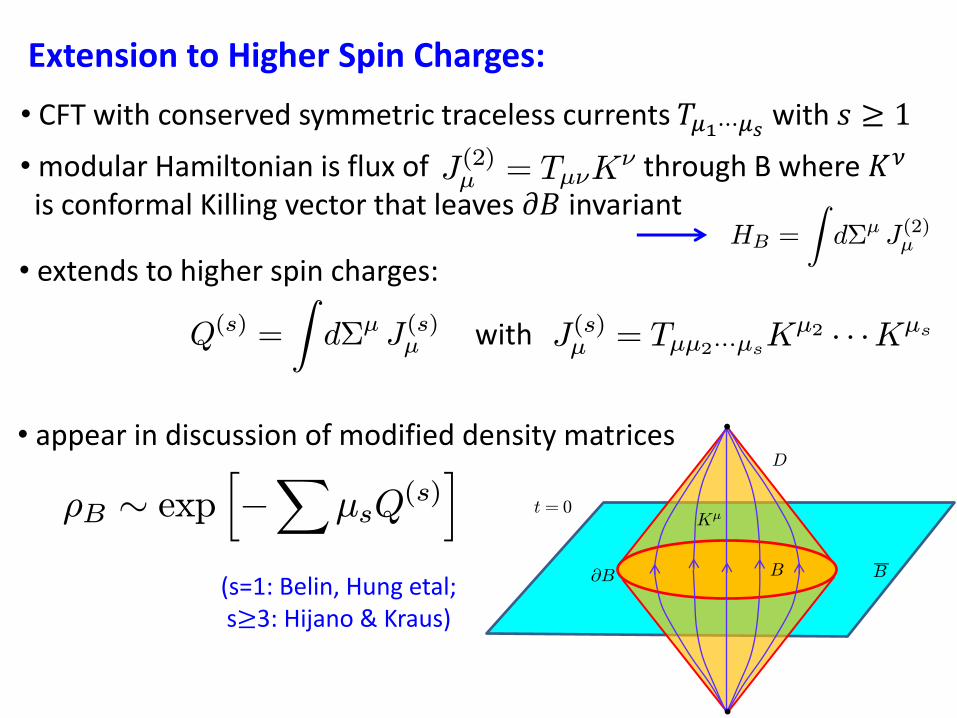
• appear in discussion of modified density matrices
½B » exph¡X
¹sQ(s)i
(s=1: Belin, Hung etal; s≥3: Hijano & Kraus)

B@B B
t = 0
•
•
K¹
D
Extension to Higher Spin Charges:
• extends to higher spin charges:
Q(s) =
Zd§¹ J(s)¹ with J(s)¹ = T¹¹2¢¢¢¹sK
¹2 ¢ ¢ ¢K¹s
Q(s) = (2¼)s¡1Z
B
dd¡1y
µR2 ¡ j~x¡ ~yj2
2R
¶s¡1Ttt:::t(~y)
• on t=0 slice, yields:
bdry-to-bulk propagator for deSitter

B@B B
t = 0
•
•
K¹
D
Extension to Higher Spin Charges:
• extends to higher spin charges:
Q(s) =
Zd§¹ J(s)¹ with J(s)¹ = T¹¹2¢¢¢¹sK
¹2 ¢ ¢ ¢K¹s
Q(s) = (2¼)s¡1Z
B
dd¡1y
µR2 ¡ j~x¡ ~yj2
2R
¶s¡1Ttt:::t(~y)
• on t=0 slice, yields:
bdry-to-bulk propagator for deSitter
• satisfies wave equation in dSd ¡r2dS ¡m2
¢Q(s) = 0
m2L2 =¡(s¡ 1)(d+ s¡ 2)
with
Q(s)

Question: Other dynamical fields in dS space?
• higher spin charges de Sitter wave equation: ¡r2dS ¡m2
¢Q(s) = 0 m2L2 =¡(s¡ 1)(d+ s¡ 2)with
• more general/generic observables? (stay tuned for part 2)

Question: Other dynamical fields in dS space?
• higher spin charges de Sitter wave equation: ¡r2dS ¡m2
¢Q(s) = 0 m2L2 =¡(s¡ 1)(d+ s¡ 2)with
• more general/generic observables? (stay tuned for part 2)
Question: Interacting fields in dS spacetime?
• how describe finite excitations? need to go beyond 1st law!!
¡r2dS ¡m2
¢±S = g ±S2 + ¢ ¢ ¢
• can higher spin charges be included, as well as 𝛿𝑆?
e.g., ???
• do we have nonlinear but local equation on dS geometry?
(stay tuned for part 2)
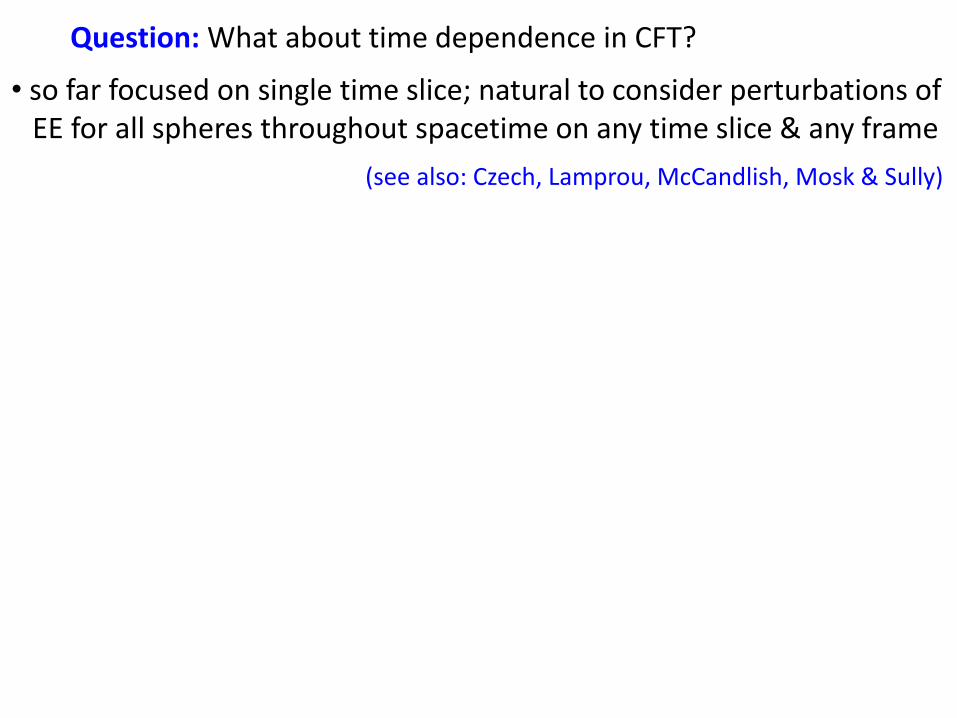
Question: What about time dependence in CFT?
• so far focused on single time slice; natural to consider perturbations of EE for all spheres throughout spacetime on any time slice & any frame
(see also: Czech, Lamprou, McCandlish, Mosk & Sully)

Question: What about time dependence in CFT?
• so far focused on single time slice; natural to consider perturbations of EE for all spheres throughout spacetime on any time slice & any frame
• how is holographic geometry modified for perturbations of EE around excited states?
• how is holographic geometry modified for perturbations of EE around CFT deformed by relevant operator?
Question: How to new construction extend beyond CFT vacuum?
(see also: Czech, Lamprou, McCandlish, Mosk & Sully)
(see also: Asplund, Callebaut & ZuKowski)
• in AdS/CFT, AdS scale set by coupling to gravity, ie, 𝐿ℓ𝑃
𝑑−2∼ 𝐶𝑇
need to understand dynamics of dS geometry
Question: How is curvature scale in dS geometry fixed?
Question: How does new framework connect to AdS/CFT?
Recap:
• 𝛿𝑆 satisfies wave equation in dSd where scale plays the role of time ¡r2dS ¡m2
¢±S = 0 m2L2 =¡dwith
• sets 𝛿𝑆 at very small 𝑅 and EE perturbations at larger scales determined by the local Lorentzian propagation into dS geometry
hTtti
• EE of excitations of CFT vacuum arranged in novel holographic manner
applies for any CFT in any d; relies only on the 1st law of entanglement; does not require strong coupling or large # dof
(dS/CFT correspondence with unitary boundary CFT?)
Question:
Is this only some “kinematic” constraint on entanglement in CFTs? or
Is there a novel re-organization of CFT where nonlocal observables yield local field theory propagating in dS spacetime?
Lots to explore!! (Stay tuned for Part 2)