wojna et al.: the devil is in the decoder the devil is in ... · wojna et al.: the devil is in the...

International Journal of Computer Vision Special Issue : BMVC 2018 manuscript No.(will be inserted by the editor)

The Devil is in the Decoder: Classification, Regression andGANs

Zbigniew Wojna · Vittorio Ferrari · Sergio Guadarrama ·Nathan Silberman · Liang-Chieh Chen · Alireza Fathi ·Jasper Uijlings

Received: date / Accepted: date

Abstract Many machine vision applications, such as

semantic segmentation and depth prediction, require

predictions for every pixel of the input image. Mod-

els for such problems usually consist of encoders which

decrease spatial resolution while learning a high-dimen-

sional representation, followed by decoders who recover

the original input resolution and result in low-dimensional

predictions. While encoders have been studied rigor-

ously, relatively few studies address the decoder side.

This paper presents an extensive comparison of a vari-

ety of decoders for a variety of pixel-wise tasks ranging

from classification, regression to synthesis. Our contri-

butions are: (1) Decoders matter: we observe significant

variance in results between different types of decoders

on various problems. (2) We introduce new residual-

like connections for decoders. (3) We introduce a novel

decoder: bilinear additive upsampling. (4) We explore

prediction artifacts.

Keywords Machine Vision · Computer Vision · Neural

Network Architectures · Decoders · 2D imagery · per-

pixel prediction · semantic segmentation · depth

prediction · GANs

Zbigniew WojnaUniversity College LondonE-mail: [email protected]

Vittorio Ferrari, Sergio Guadarrama, Nathan Silberman,Liang-Chieh Chen, Alireza Fathi, Jasper UijlingsGoogle Inc.E-mail: [email protected], [email protected],[email protected], [email protected],[email protected], [email protected]

1 Introduction

Many important machine vision applications require

predictions for every pixel of the input image. Examples

include but are not limited to: semantic segmentation

(e.g. Long et al. (2015); Tighe and Lazebnik (2010)),

boundary detection (e.g. Arbelaez et al. (2011); Ui-

jlings and Ferrari (2015)), human keypoints estimation

(e.g. Newell et al. (2016)), super-resolution (e.g. Ledig

et al. (2017)), colorization (e.g. Iizuka et al. (2016)),

depth estimation (e.g. Silberman et al. (2012)), nor-

mal surface estimation (e.g. Eigen and Fergus (2015)),

saliency prediction (e.g. Pan et al. (2016)), image gen-

eration with Generative Adversarial Networks (GANs)

(e.g. Goodfellow et al. (2014); Nguyen et al. (2017)),

and optical flow (e.g. Ilg et al. (2017)). Modern CNN-

based models for such applications are usually com-

posed of a feature extractor that decreases spatial res-

olution while learning high-dimensional representation

and a decoder that recovers the original input resolu-

tion.

Feature extractors have been rigorously studied in

the context of image classification, where individual

network improvements directly affect classification re-

sults. This makes it relatively easy to understand their

added value. Important improvements are convolutions

(LeCun et al., 1989), Rectified Linear Units (Nair and

Hinton, 2010), Local Response Normalization (Kriz-

hevsky et al., 2012), Batch Normalization (Ioffe and

Szegedy, 2015), and the use of Skip Layers (Bishop,

1995; Ripley, 1996) for Inception modules (Szegedy et al.,

2016), ResNet (He et al., 2016), and DenseNet (Huang

et al., 2017).

In contrast, decoders have been studied in relatively

few works. Furthermore, these works focus on different

problems and results are also influenced by choices and

arX

iv:1

707.

0584

7v3

[cs

.CV

] 1

9 Fe

b 20

19

2 Wojna et al.

modifications of the feature extractor. This makes it

difficult to compare existing decoder types. Our work,

therefore, presents an extensive analysis of a variety of

decoding methods on a broad range of machine vision

tasks. For each of these tasks, we fix the feature extrac-

tor which allows a direct comparison of the decoders.

In particular, we address seven machine vision tasks

spanning a classification, regression, and synthesis:

? Classification

• Semantic segmentation

• Instance edge detection

? Regression

• Human keypoints estimation

• Depth prediction

• Colorization

• Super-resolution

? Synthesis

• Image generation with generative adversarial net-

works

We make the following contributions: (1) Decoders

matter: we observe significant variance in results be-

tween different types of decoders on various problems.

(2) We introduce residual-like connections for decoders

which yield improvements across decoder types. (3) We

propose a new bilinear additive upsampling layer, which,

unlike other bilinear upsampling variants, results in con-

sistently good performance across various problem types.

(4) We investigate prediction artifacts.

2 Decoder Architecture

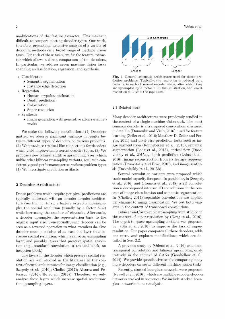
Dense problems which require per pixel predictions are

typically addressed with an encoder-decoder architec-

ture (see Fig. 1). First, a feature extractor downsam-

ples the spatial resolution (usually by a factor 8-32)

while increasing the number of channels. Afterwards,

a decoder upsamples the representation back to the

original input size. Conceptually, such decoder can be

seen as a reversed operation to what encoders do. One

decoder module consists of at least one layer that in-

creases spatial resolution, which is called an upsampling

layer, and possibly layers that preserve spatial resolu-

tion (e.g., standard convolution, a residual block, an

inception block).

The layers in the decoder which preserve spatial res-

olution are well studied in the literature in the con-

text of neural architectures for image classification (e.g.,

Szegedy et al. (2016); Chollet (2017); Alvarez and Pe-

tersson (2016); He et al. (2016)). Therefore, we only

analyze those layers which increase spatial resolution:

the upsampling layers.

Fig. 1 General schematic architecture used for dense pre-diction problems. Typically, the resolution is reduced by afactor 2 in each of several encoder steps, after which theyare upsampled by a factor 2. In this illustration, the lowestresolution is 0.125× the input size.

2.1 Related work

Many decoder architectures were previously studied in

the context of a single machine vision task. The most

common decoder is a transposed convolution, discussed

in detail in (Dumoulin and Visin, 2016), used for feature

learning (Zeiler et al., 2010; Matthew D. Zeiler and Fer-

gus, 2011) and pixel-wise prediction tasks such as im-

age segmentation (Ronneberger et al., 2015), semantic

segmentation (Long et al., 2015), optical flow (Doso-

vitskiy et al., 2015a), depth prediction (Laina et al.,

2016), image reconstruction from its feature represen-

tation (Dosovitskiy and Brox, 2016), and image synthe-

sis (Dosovitskiy et al., 2015b).

Several convolution variants were proposed which

trade model capacity for speed. In particular, in (Szegedy

et al., 2016) and (Romera et al., 2018) a 2D convolu-

tion is decomposed into two 1D convolutions in the con-text of image classification and semantic segmentation.

In (Chollet, 2017) separable convolutions are applied

per channel to image classification. We test both vari-

ants in the context of transposed convolutions.

Bilinear and/or bi-cubic upsampling were studied in

the context of super-resolution by (Dong et al., 2016).

The depth-to-space upsampling method was proposed

by (Shi et al., 2016) to improve the task of super-

resolution. Our paper compares all these decoders, adds

one extra, and explores modifications, which are de-

tailed in Sec. 2.2.

A previous study by (Odena et al., 2016) examined

transposed convolution and bilinear upsampling qual-

itatively in the context of GANs (Goodfellow et al.,

2014). We provide quantitative results comparing many

more decoders on seven different machine vision tasks.

Recently, stacked hourglass networks were proposed

(Newell et al., 2016), which are multiple encoder-decoder

networks stacked in sequence. We include stacked hour-

glass networks in our analysis.

The Devil is in the Decoder: Classification, Regression and GANs 3

2.2 Upsampling layers

Below we present and compare several ways of upsam-

pling the spatial resolution in convolution neural net-

works, a crucial part of any decoder. We limit our study

to upsampling the spatial resolution by a factor of two,

which is the most common setup in the literature (see

e.g. Ronneberger et al. (2015) and Yu and Porikli (2016)).

2.2.1 Existing upsampling layers

Transposed Convolution. Transposed convolutions are

the most commonly used upsampling layers and are

also sometimes referred to as ‘deconvolution’ or ‘upcon-

volution’ (Long et al., 2015; Dumoulin and Visin, 2016;

Zeiler et al., 2010; Dosovitskiy and Brox, 2016; Doso-

vitskiy et al., 2015a; Ronneberger et al., 2015; Laina

et al., 2016). A transposed convolution can be seen as a

reversed convolution in the sense of how the input and

output are related to each other. However, it is not an

inverse operation, since calculating the exact inverse is

an under-constrained problem and therefore ill-posed.

Transposed convolution is equivalent to interleaving the

input features with 0’s and applying a standard convo-

lutional operation. The transposed convolution is illus-

trated in Fig. 2 and 4.

Decomposed Transposed Convolution. Whereas decom-

posed transposed convolution is similar to the trans-

posed convolution, conceptually it splits the main con-

volution operation into multiple low-rank convolutions.

For images, it simulates a 2D transposed convolution

using two 1D convolutions (Fig. 5). Regarding possible

feature transformations, decomposed transposed con-

volution is strictly a subset of regular transposed con-

volution. As an advantage, the number of trainable pa-

rameters is reduced (Tab. 1).

Decomposed transposed convolution was successfully

applied in the inception architecture (Szegedy et al.,

2016), which achieved state of the art results on ILSVRC

2012 classification (Russakovsky et al., 2015). It was

also used to reduce the number of parameters of the

network in (Alvarez and Petersson, 2016).

Conv + Depth-To-Space. Depth-to-space (Shi et al.,

2016) (also called subpixel convolution) shifts the fea-

ture channels into the spatial domain as illustrated in

Fig. 3. Depth-to-space preserves perfectly all floats in-

side the high dimensional representation of the image,

as it only changes their placement. The drawback of this

approach is that it introduces alignment artifacts. To be

comparable with other upsampling layers which have

learnable parameters, before performing the depth-to-

space transformation we apply a convolution with four

times more output channels than for other upsampling

layers.

Bilinear Upsampling + Convolution. Bilinear Interpo-

lation is another conventional approach for upsampling

the spatial resolution. To be comparable to other meth-

ods, we assume there is additional convolutional op-

eration applied after the upsampling. The drawback

of this strategy is that it is both memory and com-

putationally intensive: bilinear interpolation increases

the feature size quadratically while keeping the same

amount of “information” as measured in the number

of floats. Because bilinear upsampling is followed by a

convolution, the resulting upsampling method is four

times more expensive than a transposed convolution.

Bilinear Upsampling + Separable Convolution. Sepa-

rable convolution was used to build a simple and ho-

mogeneous network architecture (Chollet, 2017) which

achieved superior results to inception-v3 (Szegedy et al.,

2016). A separable convolution consists of two opera-

tions, a per channel convolution and a pointwise convo-

lution with 1×1 kernel which mixes the channels. To in-

crease the spatial resolution, before separable convolu-

tion, we apply bilinear upsampling in our experiments.

2.2.2 Bilinear Additive Upsampling

To overcome the memory and computational problems

of bilinear upsampling, we introduce a new upsampling

layer: bilinear additive upsampling. In this layer, we

propose to do bilinear upsampling as before, but we

also add every N consecutive channels together, effec-

tively reducing the output by a factor N . This process

is illustrated in Fig. 6. Please note that this process is

deterministic and has zero tunable parameters (simi-

larly to depth-to-space upsampling, but does not cause

alignment artifacts). Therefore, to be comparable with

other upsampling methods we apply a convolution after

this upsampling method. In this paper, we choose N in

such a way that the final number of floats before and

after bilinear additive upsampling is equivalent (we up-

sample by a factor 2 and choose N = 4), which makes

the cost of this upsampling method similar to a trans-

posed convolution.

4 Wojna et al.

Fig. 2 Visual illustration of (Decomposed) Transposed Convo-lution. The resolution is increased by interleaving the featureswith zeros. Afterwards either a normal or decomposed convo-lution is applied which reduces the number of channels by afactor 4.

Fig. 3 Visual illustration of Depth-to-Space. Fist a normal con-volution is applied, keeping both the resolution and the numberof channels. Then features of each four consecutive channels arere-arranged spatially into a single channel, effectively reducingthe number of channels by a factor 4.

Fig. 4 Spatial dependency for the outputs of a Transposed Convolution with kernel size 3 and stride 2.

Fig. 5 Spatial dependency for the outputs of a Decomposed Transposed Convolution with kernel size 3 and stride 2.


Fig. 6 Visual illustration of our bilinear additive upsampling.We upsample all features and take the average over each fourconsecutive channels. For our upsampling layer this operationis followed by a convolution (not visualized).

Fig. 7 Visual illustration of our residual connection for up-sampling layers. The “identity” layer is the sum of each fourconsecutive upsampled layers in order to get the desired num-ber of channels and resolution.

2.3 Skip Connections and Residual Connections

2.3.1 Skip Connections

Skip connections have been successfully used in many

decoder architectures (Lin et al., 2017a; Ronneberger

et al., 2015; Pinheiro et al., 2016; Lin et al., 2017b;

Kendall et al., 2015). This method uses features from

the encoder in the decoder part of the same spatial res-

olution, as illustrated in Fig. 1. For our implementation

of skip connections, we apply the convolution on the last

layer of encoded features for a given spatial resolution

and concatenate them with the first layer of decoded

features (Fig. 1).

2.3.2 Residual Connections for decoders

Residual connections (He et al., 2016) have been shown

to be beneficial for a variety of tasks. However, residual

connections cannot be directly applied to upsampling

methods since the output layer has a higher spatial res-

olution than the input layer and a lower number of fea-

ture channels. In this paper, we introduce a transfor-

mation which solves both problems.

In particular, the bilinear additive upsampling method

which we introduced above (Fig. 6) transforms the in-

put layer into the desired spatial resolution and number

of channels without using any parameters. The result-

ing features contain much of the information of the orig-

inal features. Therefore, we can apply this transforma-

tion (this time without doing any convolution) and add

its result to the output of any upsampling layer, result-

ing in a residual-like connection. We present the graphi-

cal representation of the upsampling layer in Fig. 7. We

demonstrate the effectiveness of our residual connection

in Section 4.

3 Tasks and Experimental Setup

3.1 Classification

3.1.1 Semantic segmentation

We evaluate our approach on the standard PASCAL

VOC-2012 dataset (Everingham et al., 2012). We use

both the training dataset and augmented dataset (Har-

iharan et al., 2011) which together consist of 10,582

images. We evaluate on the VOC Pascal 2012 valida-

tion dataset of 1,449 images. We follow a similar setup

to Deeplab-v2 (Chen et al., 2018). As the encoder net-

work, we use ResNet-101 with stride 16. We replace

the first 7x7 convolutional layer with three 3x3 convo-

lutional layers. We use [1, 2, 4] atrous rates in the last

three convolutional layers of the block5 in Resnet-101

as in (Chen et al., 2017). We use batch normalization,

have single image pyramid by using [6, 12, 18] atrous

rates together with global feature pooling. We initialize

our model with the pre-trained weights on ImageNet

dataset with an input size of 513 × 513. Our decoder

upsamples four times by a factor 2 with a single 3x3

convolutional layer in-between. We train the network

with stochastic gradient descent on a single GPU with

a momentum of 0.9 and batch size 16. We start from

learning rate 0.007 and use a polynomial decay with the

power 0.9 for 30,000 iterations. We apply L2 regular-

ization with weight decay of 0.0001. We augment the

dataset by rescaling the images by a random factor be-

tween 0.5 and 2.0. During evaluation, we combine the

prediction from multiple scales [0.5, 0.75, 1.0, 1.25, 1.5,

1.75] and the flipped version of the input image. We

train the model using maximum likelihood estimation

per pixel (softmax cross entropy) and use mIOU (mean

Intersection Over Union) to benchmark the models.

6 Wojna et al.

Upsampling method # of parameters # of operations CommentsTransposed whIO whWHIO

Decomposed Transposed (w + h)IO (w + h)WHIO Subset of the Transposed methodConv + Depth-To-Space whI(4O) whWHI(4O)

Bilinear Upsampling + Conv whIO wh(2W )(2H)IOBilinear Upsampling + Separable whI + IO (2W )(2H)I(wh + O)

Bilinear Additive Upsampling + Conv whIO wh(2W )(2H)(I/4)O

Table 1 Comparison of different upsampling methods. W,H - feature width and height, w, h - kernel width and height, I,O- number of channels for input and output features.

3.1.2 Instance boundaries detection

For instance-wise boundaries, we use PASCAL VOC

2012 segmentation (Everingham et al., 2012). This data-

set contains 1,464 training and 1,449 validation images,

annotated with contours for 20 object classes for all in-

stances. The dataset was originally designed for seman-

tic segmentation. Therefore, only interior object pix-

els are marked, and the boundary location is recovered

from the segmentation mask. Similar to (Uijlings and

Ferrari, 2015) and (Khoreva et al., 2016), we consider

only object boundaries without distinguishing seman-

tics, treating all 20 classes as one.

As an encoder or feature extractor we use ResNet-

50 with stride 8 and atrous convolution. We initialize

from pre-trained ImageNet weights. The input to the

network is of size 321 × 321. The spatial resolution is

reduced to 41×41, after which we use 3 upsampling lay-

ers, with an additional convolutional layer in-between,

to make predictions in the original resolution.

During training, we augment the dataset by rescal-

ing the images by a random factor between 0.5 and 2.0

and random cropping. We train the network with asyn-

chronous stochastic gradient descent for 40,000 itera-

tions with a momentum of 0.9. We use a learning rate

of 0.0003 with a polynomial decay of power 0.99. We

apply L2 regularization with a weight decay of 0.0002.

We use a batch size of 5. We use sigmoid cross entropy

loss per pixel (averaged across all pixels), where 1 rep-

resents an edge pixel, and 0 represents a non-edge pixel.

We use two measures to evaluate edge detection: f-

measure for the best-fixed contour threshold across the

entire dataset and average precision (AP). During the

evaluation, predicted contour pixels within three pix-

els from ground truth pixels are assumed to be correct

(Martin et al., 2001).

3.2 Regression

3.2.1 Human keypoints estimation

We perform experiments on the MPII Human Pose data-

set (Andriluka et al., 2014) which consists of around

25k images with over 40k annotated human poses in

terms of keypoints of the locations of seven human body

parts. The images cover a wide variety of human activ-

ities. Since test annotations are not provided and since

there is no official train and validation split, we make

such split ourselves (all experiments use the same split).

In particular, we divide the training set randomly into

80% training images and 20% validation images. Fol-

lowing (Andriluka et al., 2014), we measure the Per-

centage of Correct Points with a matching threshold of

50% of the head segment length (PCKh), and report

the average over all body part on our validation set.

For the network, we re-implement the stacked hour-

glass network (Newell et al., 2016) with a few modifica-

tions. In particular, we use as input a cropped the area

around the center of human of size 353x272 pixels. We

resize predictions from every hourglass subnetwork to

their input resolution using bilinear interpolation and

then we apply a Mean Squared Error (MSE) loss. The

target values around each keypoint are based on a Gaus-

sian distribution with a standard deviation of 6 pixels

in the original input image, which we rescale such that

its highest value is 10 (which we found to work bet-

ter with MSE). We do not perform any test-time data

augmentation such as horizontal flipping.

3.2.2 Depth prediction

We apply our method to the NYUDepth v2 dataset

by (Silberman et al., 2012). We train on the entire

NYUDepth v2 raw data distribution, using the official

split. There are 209, 822 train and 187, 825 test images.

We ignore the pixels that have a depth below a thresh-

old of 0.3 meters in both training and test, as these

reads are not reliable in the Kinect sensor.

As for the encoder network, we use ResNet-50 with

stride 32, initialized with pre-trained ImageNet weights.


We use an input size of 304× 228 pixels. We apply 1x1

convolution with 1024 filters. Following (Laina et al.,

2016), we upsample four times with a convolutional

layer in between to get back to half of the original reso-

lution. Afterwards, we upsample with bilinear interpo-

lation to the original resolution (without any convolu-

tions).

We train the network with asynchronous stochas-

tic gradient descent on 3 machines with a momentum

of 0.9, batch size 16, starting from a learning rate of

0.001, decaying by 0.92 every 72926 steps and train

for 640, 000 iterations. We apply L2 regularization with

weight decay 0.0005. We augment the dataset through

random changes in brightness, hue, and saturation, through

random color removal and through mirroring.

For depth prediction, we use the reverse Huber loss

following (Laina et al., 2016).

Loss(y, y) =

{|y − y| for |y − y| <= c

|y − y|2 for |y − y| > c(1)

c =1

5max

(b,h,w)∈[1...Batch][1...Height][1...Width]|yb,h,w− ˆyb,h,w|

(2)

The reverse Huber loss is equal to the L1 norm for x ∈[−c, c] and equal to L2 norm outside this range. In every

gradient descent step, c is set to 20% of the maximal

pixel error in the batch.

For evaluation, we use the metrics from (Eigen and

Fergus, 2015), i.e., mean relative error, root mean squared

error, root mean squared log error, the percentage of

correct prediction within three relative thresholds: 1.25,

1.252 and 1.253.

3.2.3 Colorization

We train and test our models on the ImageNet dataset

(Russakovsky et al., 2015), which consists of 1, 000, 000

training images and 50, 000 validation images.

For the network architecture, we follow (Iizuka et al.,

2016), where we swap their original bilinear upsampling

method with the methods described in Section 2. In

particular, these are three upsampling steps of factor 2.

This model combines joint training of image classifi-

cation and colorization, where we are mainly interested

in the colorization part. We resize the input image to

224×224 pixels. We train the network for 30, 000 itera-

tions using the Adam optimizer with a batch size of 32

and we fix the learning rate to 1.0. We apply L2 regular-

ization with a weight decay of 0.0001. During training,

we randomly crop and randomly flip the input image.

For the skip connections, we concatenate the decoded

features with the feature extractor applied to the orig-

inal input image (as there are two encoder networks

employed on two different resolutions).

As loss function we use the averaged L1 loss for

pixel-wise color differences for the colorization part, and

a softmax cross entropy loss for the classification part.

Loss(y, y, ycl, ycl) = 10|y − y| − ycl log ycl (3)

Color predictions are made in the YPbPr color space

(luminance, blue - luminance, red - luminance). The

luminance is ignored in the loss function during both

training and evaluation as is it provided by the in-

put greyscale image. The output pixel value targets are

scaled to the range [0,1]. ycl is the one hot encoding

of the predicted class label and ycl are the predicted

classification logits.

To evaluate colorization we follow (Zhang et al.,

2016). We compute the average root mean squared er-

ror between the color channels in the predicted and

ground truth pixels. Then, for different thresholds for

root mean squared errors, we calculate the accuracy of

correctly predicted colored pixels within given range.

From these we compute the Area Under the Curve

(AUC) (Zhang et al., 2016). Additionally, we calcu-

late the top-1 and top-5 classification accuracy for the

colorized images on the ImageNet Russakovsky et al.

(2015) dataset, motivated by the assumption that bet-

ter recognition corresponds to more realistic images.

3.2.4 Super resolution

For super-resolution, we test our approach on the CelebA

dataset, which consists of 167, 483 training images and

29, 249 validation images (Liu et al., 2015). We follow

the setup from (Yu and Porikli, 2016): the input images

of the network are 16×16 images, which are created by

resizing the original images. The goal is to reconstruct

the original images which have a resolution of 128×128.

The network architecture used for super-resolution

is similar to the one from (Kim et al., 2016). We use

six ResNet-v1 blocks with 32 channels after which we

upsample by a factor of 2. We repeat this three times to

get to a target upsampling factor of 8. On top of this,

we add 2 pointwise convolutional layers with 682 chan-

nels with batch normalization in the last layer. Note

that in this problem there are only operations which

keep the current spatial resolution or which upsample

the representation. We train the network on a single

machine with 1 GPU, batch size 32, using the RM-

SProp optimizer with a momentum of 0.9, a decay of

0.95 and a batch size of 16. We fix the learning rate at

0.001 for 30000 iterations. We apply L2 regularization

8 Wojna et al.

with weight decay 0.0005. The network is trained from

scratch.

As loss we use the averaged L2 loss between the pre-

dicted residuals y and actual residuals y. The ground

truth residual y in the loss function is the difference

between original 128 × 128 target image and the pre-

dicted upsampled image. All target values are scaled to

[-1,1]. We evaluate performance using standard metrics

for super-resolution: PSNR and SSIM.

3.3 Synthesis

3.3.1 Generative Adversarial Networks

To test our decoders in the generator network for Gen-

erative Adversarial Networks (Goodfellow et al., 2014)

we follow the setup from (Lucic et al., 2017). We bench-

mark different decoders (generators) on the Cifar-10

dataset which consists of 50000 training and 10000 test-

ing 32x32 color images. Additionally, we also test our

approach on the CelebA dataset described in Sec. 3.2.4.

For Cifar-10 we use the GAN architecture with spec-

tral normalization of Miyato et al. (2018). For CelebA,

we use the InfoGan architecture (Chen et al., 2016). For

both networks, we replace the transposed convolutions

in the generator with our upsampling layers and add

3x3 convolutional layers between them. In the discrim-

inator network, we do not use batch normalization. We

train the model with batch size 64 through 200k itera-

tions on a single GPU using the Adam optimizer. We

perform extensive hyperparameter search for each of

the studied decoder architectures: We vary the learning

rate from a logarithmic scale between [0.00001, 0.01], we

vary the beta1 parameter for the Adam optimizer from

range [0, 1], and the λ used in the gradient penalty term

(Eq. (4)) from a logarithmic scale in range [-1, 2]. We

try both 1 and 5 discriminator updates per generator

update.

As the discriminator and generator loss functions

we are using the Wasserstein GAN Loss with Gradient

Penalty (Gulrajani et al., 2017):

LD =− Ex∼pd[D(x)] + Ex∼pg

[D(x)] +

λEx∼pg [(||∇D(αx+ (1− αx))||2 − 1)2] (4)

LG =− Ex∼pg [D(x)] (5)

where pd is data distribution, pg is the generator

output distribution, and D is the output of the dis-

criminator. α is uniformly sampled in every iteration

from range [0, 1].

We evaluate the performance of the generator ar-

chitectures using the Frechet Inception Distance (FID)

(Heusel et al., 2017).

4 Results

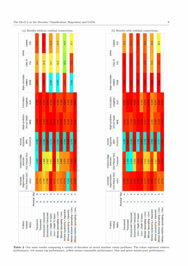
We first compare the upsampling types described in

Section 2.2 without residual connections (Tab. 1(a)).

Next, we discuss the benefits of adding our residual

connections (Tab. 1(b)). Since all evaluation metrics are

highly correlated, this table only reports a single metric

per problem. A table with all metrics can be found in

the supplementary material.

4.1 Results without residual-like connections.

For semantic segmentation, the depth-to-space trans-

formation is the best upsampling method. For instance

edge detection and human keypoints estimation, the

skip-layers are necessary to get good results. For in-

stance edge detection, the best performance is obtained

by transposed, depth-to-space, and bilinear additive up-

sampling. For human keypoints estimation, the hour-

glass network uses skip-layers by default and all types

of upsampling layers are about as good. For both depth

prediction and colorization, all upsampling methods per-

form similarly, and the specific choice of upsampling

matters little. For super-resolution, networks with skip-

layers are not possible because there are no encoder

modules which high-resolution (and relatively low-seman-

tic) features. Therefore, this problem has no skip-layer

entries. Regarding performance, only all transposed vari-

ants perform well on this task; other layers do not.

Similarly to super-resolution, GANs have no encoder

and therefore it is not possible to have skip connec-

tions. Separable convolutions perform very poorly on

this task. There is no single decoder which performs well

on both Cifar 10 and CelebA datasets: bilinear additive

upsampling performs well on Cifar 10, but poorly in

CelebA. In contrast, decomposed transposed performs

well on CelebA, but poorly on Cifar 10.

Generalizing over problems, we see that no single

upsampling scheme provides consistently good results

across all the tasks.

4.2 Results with residual-like connections

Next, we add our residual-like connections to all upsam-

pling methods. Results are presented in Tab. 1(b). For


(a) Results without residual connections. (b) Results with residual connections.

Table 2 Our main results comparing a variety of decoders on seven machine vision problems. The colors represent relativeperformance: red means top performance, yellow means reasonable performance, blue and green means poor performance.

10 Wojna et al.

Method Measure Our method Recent work Recent work

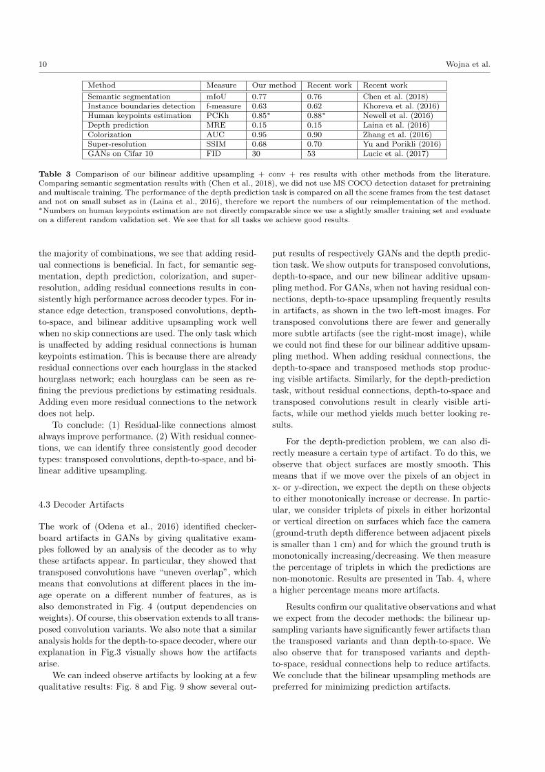
Semantic segmentation mIoU 0.77 0.76 Chen et al. (2018)Instance boundaries detection f-measure 0.63 0.62 Khoreva et al. (2016)Human keypoints estimation PCKh 0.85∗ 0.88∗ Newell et al. (2016)Depth prediction MRE 0.15 0.15 Laina et al. (2016)Colorization AUC 0.95 0.90 Zhang et al. (2016)Super-resolution SSIM 0.68 0.70 Yu and Porikli (2016)GANs on Cifar 10 FID 30 53 Lucic et al. (2017)

Table 3 Comparison of our bilinear additive upsampling + conv + res results with other methods from the literature.Comparing semantic segmentation results with (Chen et al., 2018), we did not use MS COCO detection dataset for pretrainingand multiscale training. The performance of the depth prediction task is compared on all the scene frames from the test datasetand not on small subset as in (Laina et al., 2016), therefore we report the numbers of our reimplementation of the method.∗Numbers on human keypoints estimation are not directly comparable since we use a slightly smaller training set and evaluateon a different random validation set. We see that for all tasks we achieve good results.

the majority of combinations, we see that adding resid-

ual connections is beneficial. In fact, for semantic seg-

mentation, depth prediction, colorization, and super-

resolution, adding residual connections results in con-

sistently high performance across decoder types. For in-

stance edge detection, transposed convolutions, depth-

to-space, and bilinear additive upsampling work well

when no skip connections are used. The only task which

is unaffected by adding residual connections is human

keypoints estimation. This is because there are already

residual connections over each hourglass in the stacked

hourglass network; each hourglass can be seen as re-

fining the previous predictions by estimating residuals.

Adding even more residual connections to the network

does not help.

To conclude: (1) Residual-like connections almost

always improve performance. (2) With residual connec-

tions, we can identify three consistently good decoder

types: transposed convolutions, depth-to-space, and bi-linear additive upsampling.

4.3 Decoder Artifacts

The work of (Odena et al., 2016) identified checker-

board artifacts in GANs by giving qualitative exam-

ples followed by an analysis of the decoder as to why

these artifacts appear. In particular, they showed that

transposed convolutions have “uneven overlap”, which

means that convolutions at different places in the im-

age operate on a different number of features, as is

also demonstrated in Fig. 4 (output dependencies on

weights). Of course, this observation extends to all trans-

posed convolution variants. We also note that a similar

analysis holds for the depth-to-space decoder, where our

explanation in Fig.3 visually shows how the artifacts

arise.

We can indeed observe artifacts by looking at a few

qualitative results: Fig. 8 and Fig. 9 show several out-

put results of respectively GANs and the depth predic-

tion task. We show outputs for transposed convolutions,

depth-to-space, and our new bilinear additive upsam-

pling method. For GANs, when not having residual con-

nections, depth-to-space upsampling frequently results

in artifacts, as shown in the two left-most images. For

transposed convolutions there are fewer and generally

more subtle artifacts (see the right-most image), while

we could not find these for our bilinear additive upsam-

pling method. When adding residual connections, the

depth-to-space and transposed methods stop produc-

ing visible artifacts. Similarly, for the depth-prediction

task, without residual connections, depth-to-space and

transposed convolutions result in clearly visible arti-

facts, while our method yields much better looking re-

sults.

For the depth-prediction problem, we can also di-

rectly measure a certain type of artifact. To do this, we

observe that object surfaces are mostly smooth. This

means that if we move over the pixels of an object in

x- or y-direction, we expect the depth on these objects

to either monotonically increase or decrease. In partic-

ular, we consider triplets of pixels in either horizontal

or vertical direction on surfaces which face the camera

(ground-truth depth difference between adjacent pixels

is smaller than 1 cm) and for which the ground truth is

monotonically increasing/decreasing. We then measure

the percentage of triplets in which the predictions are

non-monotonic. Results are presented in Tab. 4, where

a higher percentage means more artifacts.

Results confirm our qualitative observations and what

we expect from the decoder methods: the bilinear up-

sampling variants have significantly fewer artifacts than

the transposed variants and than depth-to-space. We

also observe that for transposed variants and depth-

to-space, residual connections help to reduce artifacts.

We conclude that the bilinear upsampling methods are

preferred for minimizing prediction artifacts.


Depth-to-Space Transposed Bilinear Additive Upsampling

no residual

with residual

Fig. 8 Visualizations of GANs

Upsampling layer Skip Res artifacts artifactsx-axis y-axis

Transposed N N 27.6% 24.8%Transposed Y N 30.6% 23.5%Transposed N Y 23.1% 21.9%Transposed Y Y 22.8% 22.8%Dec. Transposed N N 27.0% 24.1%Dec. Transposed Y N 33.4% 24.0%Dec. Transposed N Y 25.5% 23.9%Dec. Transposed Y Y 24.5% 24.1%Depth-To-Space N N 28.4% 26.9%Depth-To-Space Y N 26.3% 23.2%Depth-To-Space N Y 25.6% 23.7%Depth-To-Space Y Y 24.2% 22.9%Bilinear Ups. + Conv. N N 14.3% 14.6%Bilinear Ups. + Conv. Y N 19.5% 19.5%Bilinear Ups. + Conv. N Y 14.7% 14.8%Bilinear Ups. + Conv. Y Y 17.4% 18.3%Bilinear Ups. + Sep. N N 13.8% 14.6%Bilinear Ups. + Sep. Y N 20.5% 20.3%Bilinear Ups. + Sep. N Y 17.3% 16.0%Bilinear Ups. + Sep. Y Y 19.7% 18.3%Bilinear Add. Ups. N N 14.8% 15.2%Bilinear Add. Ups. Y N 19.0% 17.7%Bilinear Add. Ups. N Y 14.7% 15.0%Bilinear Add. Ups. Y Y 17.5% 18.4%

Table 4 Analysis of the artifacts for depth regression for1000 test images, totalling approximately 27 million tripletsper experiment.

4.4 Nearest Neighbour and Bicubic Upsampling

The upsampling layers in our study used bilinear up-

sampling if applicable. But one can also use nearest

neighbour upsampling (e.g. Berthelot et al. (2017); Jia

et al. (2017); Odena et al. (2016)) or bicubic upsam-

pling (e.g. Dong et al. (2016); Hui et al. (2016); Kim

et al. (2016); Odena et al. (2016)). We performed two

small experiments to examine these alternatives.

In particular, on the Human keypoints estimation

task (Sec. 3.2.1) we started from the bilinear upsam-

pling + conv method with residual connections and

skip layers. Then we changed the bilinear upsampling to

nearest neighbour and bicubic. Results are in Tab. 5. As

can be seen, the nearest neighbour sampling is slightly

worse than bilinear and bicubic, which perform about

the same.

Fig. 9 Input image and errors for three different models.Top row: input image. Second row: Transposed. Third row:Depth-to-Space. Fourth row: Bilinear additive upsampling.We observe that our proposed upsampling method producessmoother results with less arifacts.

Res Skip PCK/0.50NN Ups. + Conv Y Y 0.846Bilinear Ups. + Conv Y Y 0.854Bicubic Ups. Conv Y Y 0.855

Table 5 Comparison of Nearest Neighbour Upsamping, Bi-linear Upsampling, and Bicubic Usampling on Human Key-point Estimation.

Res Skip FIDNN Ups. + Conv Y N 28.0Bilinear Ups. + Conv Y N 29.8Bicubic Ups. Conv Y N 28.1

Table 6 Comparison of Nearest Neighbour Upsamping, Bi-linear Upsampling, and Bicubic Usampling on generating syn-thetic images using GANs for Cifar 10.

We also compared the same three decoder types to

synthesize data using GANs (Sec. 3.3.1) on Cifar 10

(without skip connections since these are not applica-

ble). Results are in Tab. 6. As can be seen, nearest

neighbour upsampling and bicubic have similar perfor-

12 Wojna et al.

mance. This is in contrast to Odena et al. (2016) who

found that nearest neighbour upsampling worked better

than bicubic upsampling. In Odena et al. (2016) they

suggested that their results could have been caused by

the hyperparameters being optimized for nearest neigh-

bour upsampling. Our result seems to confirm this. Bi-

linear upsampling performs slightly worse than the other

two methods.

To conclude, in both experiments the differences be-

tween upsampling methods are rather small. Bicubic

upsampling slightly outperforms the two others. Intu-

itively, this is the more accurate non-parametric upsam-

pling method but one that has a higher computational

cost.

5 Conclusions

This paper provided an extensive evaluation for differ-

ent decoder types on a broad range of machine vision

applications. Our results demonstrate: (1) Decoders mat-

ter: there are significant performance differences among

different decoders depending on the problem at hand.

(2) We introduced residual-like connections which, in

the majority of cases, yield good improvements when

added to any upsampling layer. (3) We introduced the

bilinear additive upsampling layer, which strikes a right

balance between the number of parameters and accu-

racy. Unlike the other bilinear variants, it gives con-

sistently good performance across all applications. (4)

Transposed convolution variants and depth-to-space de-

coders have considerable prediction artifacts, while bi-

linear upsampling variants suffer from this much less.

(5) Finally, when using residual connections, transposed

convolutions, depth-to-space, and our bilinear additive

upsampling give consistently strong quantitative results

across all problems. However, since our bilinear additive

upsampling suffers much less from prediction artifacts,

it should be the upsampling method of choice.

References

Jose M. Alvarez and Lars Petersson. Decomposeme:

Simplifying convnets for end-to-end learning. CoRR,

abs/1606.05426, 2016. URL http://arxiv.org/

abs/1606.05426.

Mykhaylo Andriluka, Leonid Pishchulin, Peter Gehler,

and Bernt Schiele. 2d human pose estimation: New

benchmark and state of the art analysis. In CVPR,

2014.

P. Arbelaez, M. Maire, C. Fowlkes, and J. Malik. Con-

tour detection and hierarchical image segmentation.

IEEE Trans. on PAMI, 2011.

David Berthelot, Tom Schumm, and Luke Metz. BE-

GAN: Boundary equilibrium generative adversarial

networks. In ArXiv, 2017.

C. M. Bishop. Neural networks for pattern recognition.

Oxford university press, 1995.

Liang-Chieh Chen, George Papandreou, Flo-

rian Schroff, and Hartwig Adam. Rethinking

atrous convolution for semantic image segmen-

tation. CoRR, abs/1706.05587, 2017. URL

http://arxiv.org/abs/1706.05587.

Liang-Chieh Chen, George Papandreou, Iasonas Kokki-

nos, Kevin Murphy, and Alan L Yuille. Deeplab: Se-

mantic image segmentation with deep convolutional

nets, atrous convolution, and fully connected crfs.

IEEE transactions on pattern analysis and machine

intelligence, 40(4):834–848, 2018.

Xi Chen, Xi Chen, Yan Duan, Rein Houthooft, John

Schulman, Ilya Sutskever, and Pieter Abbeel. In-

fogan: Interpretable representation learning by in-

formation maximizing generative adversarial nets.

In Daniel D. Lee, Masashi Sugiyama, Ulrike von

Luxburg, Isabelle Guyon, and Roman Garnett, ed-

itors, Advances in Neural Information Processing

Systems 29: Annual Conference on Neural Informa-

tion Processing Systems 2016, December 5-10, 2016,

Barcelona, Spain, pages 2172–2180, 2016.

Francois Chollet. Xception: Deep learning with depth-

wise separable convolutions. In 2017 IEEE Confer-

ence on Computer Vision and Pattern Recognition,

CVPR 2017, Honolulu, HI, USA, July 21-26, 2017,

pages 1800–1807, 2017. doi: 10.1109/CVPR.2017.

195. URL https://doi.org/10.1109/CVPR.2017.

195.

Chao Dong, Chen Change Loy, Kaiming He, and Xi-

aoou Tang. Image super-resolution using deep con-

volutional networks. IEEE Transactions on Pattern

Analysis and Machine Intelligence, 38, 2016.

Alexey Dosovitskiy and Thomas Brox. Inverting visual

representations with convolutional networks. In Pro-

ceedings of the IEEE Conference on Computer Vision

and Pattern Recognition, pages 4829–4837, 2016.

Alexey Dosovitskiy, Philipp Fischer, Eddy Ilg, Philip

Hausser, Caner Hazirbas, Vladimir Golkov, Patrick

van der Smagt, Daniel Cremers, and Thomas Brox.

Flownet: Learning optical flow with convolutional

networks. In Proceedings of the IEEE International

Conference on Computer Vision, pages 2758–2766,

2015a.

Alexey Dosovitskiy, Jost Tobias Springenberg, and

Thomas Brox. Learning to generate chairs with con-

volutional neural networks. In CVPR, 2015b.

Vincent Dumoulin and Francesco Visin. A guide to

convolution arithmetic for deep learning. CoRR,

http://arxiv.org/abs/1606.05426



https://doi.org/10.1109/CVPR.2017.195



abs/1603.07285, 2016. URL http://arxiv.org/

abs/1603.07285.

David Eigen and Rob Fergus. Predicting depth, surface

normals and semantic labels with a common multi-

scale convolutional architecture. In Proceedings of the

IEEE International Conference on Computer Vision,

pages 2650–2658, 2015.

M. Everingham, L. Van Gool, C. K. I. Williams,

J. Winn, and A. Zisserman. The PASCAL Visual

Object Classes Challenge 2012 (VOC2012) Results,

2012.

Ian J. Goodfellow, Jean Pouget-Abadie, Mehdi

Mirza, Bing Xu, David Warde-Farley, Sherjil Ozair,

Aaron C. Courville, and Yoshua Bengio. Generative

adversarial nets. NIPS, 2014.

Ishaan Gulrajani, Faruk Ahmed, Martın Ar-

jovsky, Vincent Dumoulin, and Aaron C.

Courville. Improved training of wasserstein

gans. In Guyon et al. (2017), pages 5769–

5779. URL http://papers.nips.cc/paper/

7159-improved-training-of-wasserstein-gans.

Isabelle Guyon, Ulrike von Luxburg, Samy Bengio,

Hanna M. Wallach, Rob Fergus, S. V. N. Vish-

wanathan, and Roman Garnett, editors. Advances

in Neural Information Processing Systems 30: An-

nual Conference on Neural Information Processing

Systems 2017, 4-9 December 2017, Long Beach, CA,

USA, 2017.

Bharath Hariharan, Pablo Arbelaez, Lubomir Bour-

dev, Subhransu Maji, and Jitendra Malik. Semantic

contours from inverse detectors. In Computer Vi-

sion (ICCV), 2011 IEEE International Conference

on, pages 991–998. IEEE, 2011.

Kaiming He, Xiangyu Zhang, Shaoqing Ren, and Jian

Sun. Deep residual learning for image recognition.

In Proceedings of the IEEE conference on computer

vision and pattern recognition, pages 770–778, 2016.

Martin Heusel, Hubert Ramsauer, Thomas Un-

terthiner, Bernhard Nessler, and Sepp Hochreiter.

Gans trained by a two time-scale update rule con-

verge to a local nash equilibrium. In Guyon et al.

(2017), pages 6629–6640.

Gao Huang, Zhuang Liu, Laurens van der Maaten, and

Kilian Q Weinberger. Densely connected convolu-

tional networks. In Proceedings of the IEEE con-

ference on computer vision and pattern recognition,

volume 1, page 3, 2017.

Tak-Wai Hui, Chen Change Loy, and Xiaoou Tang.

Depth map super-resolution by deep multi-scale

guidance. In ECCV, 2016.

Satoshi Iizuka, Edgar Simo-Serra, and Hiroshi Ishikawa.

Let there be color!: joint end-to-end learning of global

and local image priors for automatic image coloriza-

tion with simultaneous classification. ACM Transac-

tions on Graphics (TOG), 35(4):110, 2016.

Eddy Ilg, Nikolaus Mayer, Tonmoy Saikia, Margret Ke-

uper, Alexey Dosovitskiy, and Thomas Brox. Flownet

2.0: Evolution of optical flow estimation with deep

networks. In 2017 IEEE Conference on Computer

Vision and Pattern Recognition, CVPR 2017, Hon-

olulu, HI, USA, July 21-26, 2017, pages 1647–1655,

2017. doi: 10.1109/CVPR.2017.179. URL https:

//doi.org/10.1109/CVPR.2017.179.

S. Ioffe and C. Szegedy. Batch normalization: Accel-

erating deep network training by reducing internal

covariate shift. In ICML, 2015.

Xu Jia, Hong Chang, and Tinne Tuytelaars. Super-

resolution with deep adaptive image resampling. In

ArXiv, 2017.

Alex Kendall, Vijay Badrinarayanan, and Roberto

Cipolla. Bayesian segnet: Model uncertainty in deep

convolutional encoder-decoder architectures for scene

understanding. CoRR, abs/1511.02680, 2015. URL

http://arxiv.org/abs/1511.02680.

Anna Khoreva, Rodrigo Benenson, Mohamed Omran,

Matthias Hein, and Bernt Schiele. Weakly super-

vised object boundaries. In Proceedings of the IEEE

Conference on Computer Vision and Pattern Recog-

nition, pages 183–192, 2016.

Jiwon Kim, Jung Kwon Lee, and Kyoung Mu Lee. Ac-

curate image super-resolution using very deep convo-

lutional networks. In Proceedings of the IEEE Con-

ference on Computer Vision and Pattern Recogni-

tion, pages 1646–1654, 2016.

A. Krizhevsky, I. Sutskever, and G. E. Hinton. Im-

agenet classification with deep convolutional neural

networks. In NIPS, 2012.

Iro Laina, Christian Rupprecht, Vasileios Belagiannis,

Federico Tombari, and Nassir Navab. Deeper depth

prediction with fully convolutional residual networks.

In 3D Vision (3DV), 2016 Fourth International Con-

ference on, pages 239–248. IEEE, 2016.

Yann LeCun, Bernhard Boser, John S Denker, Don-

nie Henderson, Richard E Howard, Wayne Hubbard,

and Lawrence D Jackel. Backpropagation applied to

handwritten zip code recognition. Neural computa-

tion, 1(4):541–551, 1989.

Christian Ledig, Lucas Theis, Ferenc Huszar, Jose Ca-

ballero, Andrew Cunningham, Alejandro Acosta, An-

drew P Aitken, Alykhan Tejani, Johannes Totz, Ze-

han Wang, et al. Photo-realistic single image super-

resolution using a generative adversarial network. In

CVPR, volume 2, page 4, 2017.

Guosheng Lin, Anton Milan, Chunhua Shen, and Ian D

Reid. Refinenet: Multi-path refinement networks for

high-resolution semantic segmentation. In Cvpr, vol-



http://papers.nips.cc/paper/7159-improved-training-of-wasserstein-gans

http://papers.nips.cc/paper/7159-improved-training-of-wasserstein-gans




14 Wojna et al.

ume 1, page 5, 2017a.

Tsung-Yi Lin, Piotr Dollar, Ross B Girshick, Kaim-

ing He, Bharath Hariharan, and Serge J Belongie.

Feature pyramid networks for object detection. In

CVPR, volume 1, page 4, 2017b.

Ziwei Liu, Ping Luo, Xiaogang Wang, and Xiaoou Tang.

Deep learning face attributes in the wild. In Proceed-

ings of International Conference on Computer Vision

(ICCV), December 2015.

Jonathan Long, Evan Shelhamer, and Trevor Darrell.

Fully convolutional networks for semantic segmenta-

tion. In Proceedings of the IEEE Conference on Com-

puter Vision and Pattern Recognition, pages 3431–

3440, 2015.

Mario Lucic, Karol Kurach, Marcin Michalski, Sylvain

Gelly, and Olivier Bousquet. Are gans created equal?

A large-scale study. CoRR, abs/1711.10337, 2017.

URL http://arxiv.org/abs/1711.10337.

David Martin, Charless Fowlkes, Doron Tal, and Jiten-

dra Malik. A database of human segmented natural

images and its application to evaluating segmenta-

tion algorithms and measuring ecological statistics.

In Computer Vision, 2001. ICCV 2001. Proceedings.

Eighth IEEE International Conference on, volume 2,

pages 416–423. IEEE, 2001.

Graham W. Taylor Matthew D. Zeiler and Rob Fergus.

Adaptive deconvolutional networks for mid and high

level feature learning. In ICCV, 2011.

Takeru Miyato, Toshiki Kataoka, Masanori Koyama,

and Yuichi Yoshida. Spectral normalization for gen-

erative adversarial networks. In International Con-

ference on Learning Representations, 2018. URL

https://openreview.net/forum?id=B1QRgziT-.

Vinod Nair and Geoffrey E Hinton. Rectified linear

units improve restricted boltzmann machines. In Pro-

ceedings of the 27th international conference on ma-

chine learning (ICML-10), pages 807–814, 2010.

Alejandro Newell, Kaiyu Yang, and Jia Deng. Stacked

hourglass networks for human pose estimation. In

European Conference on Computer Vision, pages

483–499. Springer, 2016.

Anh Nguyen, Jeff Clune, Yoshua Bengio, Alexey Doso-

vitskiy, and Jason Yosinski. Plug & play genera-

tive networks: Conditional iterative generation of im-

ages in latent space. In 2017 IEEE Conference on

Computer Vision and Pattern Recognition, CVPR

2017, Honolulu, HI, USA, July 21-26, 2017, pages

3510–3520, 2017. doi: 10.1109/CVPR.2017.374. URL

https://doi.org/10.1109/CVPR.2017.374.

Augustus Odena, Vincent Dumoulin, and Chris Olah.

Deconvolution and checkerboard artifacts. Distill, 1

(10):e3, 2016.

Junting Pan, Elisa Sayrol, Xavier Giro-i Nieto, Kevin

McGuinness, and Noel E O’Connor. Shallow and

deep convolutional networks for saliency prediction.

In Proceedings of the IEEE Conference on Computer

Vision and Pattern Recognition, pages 598–606, 2016.

Pedro O Pinheiro, Tsung-Yi Lin, Ronan Collobert, and

Piotr Dollar. Learning to refine object segments. In

European Conference on Computer Vision, pages 75–

91. Springer, 2016.

B. D. Ripley. Pattern recognition and neural networks.

Cambridge university press, 1996.

Eduardo Romera, Jose Alvarez, Luis Miguel Bergasa,

and Roberto Arroyo. Erfnet: Efficient residual fac-

torized convnet for real-time semantic segmenta-

tion. IEEE Transactions on Intelligent Transporta-

tion Systems, 19:263–272, 2018.

Olaf Ronneberger, Philipp Fischer, and Thomas Brox.

U-net: Convolutional networks for biomedical image

segmentation. In International Conference on Med-

ical Image Computing and Computer-Assisted Inter-

vention, pages 234–241. Springer, 2015.

Olga Russakovsky, Jia Deng, Hao Su, Jonathan Krause,

Sanjeev Satheesh, Sean Ma, Zhiheng Huang, An-

drej Karpathy, Aditya Khosla, Michael Bernstein,

Alexander C. Berg, and Li Fei-Fei. ImageNet Large

Scale Visual Recognition Challenge. International

Journal of Computer Vision (IJCV), 115(3):211–252,

2015. doi: 10.1007/s11263-015-0816-y.

Wenzhe Shi, Jose Caballero, Ferenc Huszar, Johannes

Totz, Andrew P Aitken, Rob Bishop, Daniel Rueck-

ert, and Zehan Wang. Real-time single image and

video super-resolution using an efficient sub-pixel

convolutional neural network. In Proceedings of the

IEEE Conference on Computer Vision and Pattern

Recognition, pages 1874–1883, 2016.

Nathan Silberman, Derek Hoiem, Pushmeet Kohli, and

Rob Fergus. Indoor segmentation and support infer-

ence from rgbd images. In ECCV, 2012.

Christian Szegedy, Vincent Vanhoucke, Sergey Ioffe,

Jon Shlens, and Zbigniew Wojna. Rethinking the

inception architecture for computer vision. In Pro-

ceedings of the IEEE Conference on Computer Vision

and Pattern Recognition, pages 2818–2826, 2016.

J. Tighe and S. Lazebnik. Superparsing: Scalable

nonparametric image parsing with superpixels. In

ECCV, 2010.

Jasper RR Uijlings and Vittorio Ferrari. Situational ob-

ject boundary detection. In Proceedings of the IEEE

Conference on Computer Vision and Pattern Recog-

nition, pages 4712–4721, 2015.

Xin Yu and Fatih Porikli. Ultra-resolving face im-

ages by discriminative generative networks. In Eu-

ropean Conference on Computer Vision, pages 318–


https://openreview.net/forum?id=B1QRgziT-



333. Springer, 2016.

Matthew D Zeiler, Dilip Krishnan, Graham W Taylor,

and Rob Fergus. Deconvolutional networks. In Com-

puter Vision and Pattern Recognition (CVPR), 2010

IEEE Conference on, pages 2528–2535. IEEE, 2010.

Richard Zhang, Phillip Isola, and Alexei A Efros. Col-

orful image colorization. In European Conference on

Computer Vision, pages 649–666. Springer, 2016.

16 Wojna et al.

6 Appendix


(a) Results without residualconnections.

(b) Results with residual con-nections.

Table 7 Our main results comparing a variety of decoders on seven machine vision problems. The colors represent relativeperformance: red means top performance, yellow means reasonable performance, blue and green means poor performance.

wojna et al.: the devil is in the decoder the devil is in ... · wojna et al.: the devil is in the...

Documents