DI

SC

US

SI

ON

P

AP

ER

S

ER

IE

S

Forschungsinstitut zur Zukunft der ArbeitInstitute for the Study of Labor

Women, Children and Patience:Experimental Evidence from Indian Villages

IZA DP No. 4241

June 2009

Michal BauerJulie Chytilová

Women, Children and Patience:

Experimental Evidence from Indian Villages

Michal Bauer Charles University

and IZA

Julie Chytilová Charles University

Discussion Paper No. 4241 June 2009

IZA

P.O. Box 7240 53072 Bonn

Germany

Phone: +49-228-3894-0 Fax: +49-228-3894-180

E-mail: iza@iza.org

Any opinions expressed here are those of the author(s) and not those of IZA. Research published in this series may include views on policy, but the institute itself takes no institutional policy positions. The Institute for the Study of Labor (IZA) in Bonn is a local and virtual international research center and a place of communication between science, politics and business. IZA is an independent nonprofit organization supported by Deutsche Post Foundation. The center is associated with the University of Bonn and offers a stimulating research environment through its international network, workshops and conferences, data service, project support, research visits and doctoral program. IZA engages in (i) original and internationally competitive research in all fields of labor economics, (ii) development of policy concepts, and (iii) dissemination of research results and concepts to the interested public. IZA Discussion Papers often represent preliminary work and are circulated to encourage discussion. Citation of such a paper should account for its provisional character. A revised version may be available directly from the author.

IZA Discussion Paper No. 4241 June 2009

ABSTRACT

Women, Children and Patience: Experimental Evidence from Indian Villages*

In this paper we study the link between women’s responsibility for children and their preferences. We use a large random sample of individuals living in rural India, incentive compatible measures of patience and risk aversion, and detailed survey data. We find more patient choices among women who have a higher number of children. The age of children matters: The link with patience is specific for children below 18 years old, and the highest level of patience is associated with having three children. We do not observe this link among men. Taken together, we find significant gender differences in patience that are predicted by a higher number of children. The results are robust to controlling for age, education, income constraints, and individual and location characteristics. These findings suggest an important context when the spending preferences of spouses diverge, and support the view that empowering women in developing countries should lead to more future-oriented choices of households. JEL Classification: C93, D13, D91, 012 Keywords: time discounting, gender, children, experiment, India Corresponding author: Michal Bauer Institute of Economic Studies Charles University in Prague Opletalova 26 Prague 1, 110 00 Czech Republic E-mail: bauerm@fsv.cuni.cz

* We thank BPKS and Caritas Prague for collaboration on the field work and J. Kabatová, D. Mascarenhas, S. Crasta and L. Perreira for excellent research assistance. We thank R. Fernandez, R. Filer, B. Forbes, I. Gang, D. Malunda, A. Mayer, J. Morduch, D. Munich, A. Ortmann, S. Pratap, D. Ray, D. Thomas and participants of several conferences and seminars for valuable comments in various stages of the project. We appreciate the financial support by a grant from the CERGE-EI Foundation under a program of the Global Development Network and by the IES/Charles University research framework 2005-10. All opinions and errors are our own.

3

I. Introduction

Research has shown that individual decisions may vary by gender. In the context of developing

countries, women have often been observed to make more development-germane choices than

men, leading many to highlight gender equality as a powerful mean of human development in

poor countries (United Nations 2005). The underlying causes of these differences remain

unclear, but a growing body of evidence suggests that women place a relatively greater weight

on child welfare (Miller 2008). It has been reported that a greater income share in the hands of

women leads to higher child survival probability (Thomas 1990) and enhances the

anthropometric status of girls (Duflo 2003)1,2. Recently, Rubalcava, Teruel and Thomas (2009)

find that women are more likely to spend their income on investments in children, and they

link these allocations with direct measures of inter-temporal preference, which indicate that

women are more patient than men.

Despite its relevance for studying potential causes of these differences, the question of

whether the preference heterogeneity between men and women is stable or if it varies with

observable characteristics has received relatively little attention. Women in rural India, as well

as other low-income communities, are typically housewives taking care of their families and

most of their activities are centered on their children. Thus, a natural, though unexplored, area

for understanding women’s preferences is their responsibility for their children’s well being.

This paper tests whether individual time discounting and risk aversion is related to the

number and composition of children, and whether the potential link is similar for men and for

women. We use a random sample of more than 500 individuals living in rural Karnataka, India.

Subjects made choices in paid experimental tasks, which provide incentive compatible

measures of risk aversion, impatience and time preference reversals. Measures of risk aversion

involved choices over lotteries. Measures of time discounting involved making choices over

1 Despite recent interest in the context of developing countries, the idea that female empowerment leads to higher

investments in child quality is quite common in theoretical studies on the history of developed countries (Doepke

and Tertilt forthcoming; Edlund and Lagerlof 2004). Miller (2008) presents evidence on how suffrage rights for

American women lead to an increase in public health spending and child survival rates in the U.S. 2 Development practitioners made similar observations. Based on the positive experience of the Grameen Bank

with regards to providing credit to women, Muhammad Yunus (2002, p.374) argues: “…women have a longer

vision than men. Men are more likely to enjoy what they’ve got right away, and they are generally more

impulsive. But a woman is more likely to have a very consistent vision for the future. She wants a better life and

to build security for her and for her family.”

4

tradeoffs between earlier payments and with a three-month delay. One battery of inter-temporal

choices was set in an earlier time frame and the second one in a future time frame.

Experimental responses are complemented with a detailed survey of individual economic and

demographic characteristics, including the number and the gender and age composition of the

children.

We find that women make more patient choices than men. The main finding is that

women’s patience is systematically related to the number of children. Women with more

children below 18 years of age make more patient choices in both the current and future time

frame. This relationship holds over the range of children that is common for Indian families

and in our sample (between zero and four children). We do not observe a link between children

and patience for men. Hence, gender heterogeneity in patience increases with a higher number

of children. These results are robust to controlling for individual characteristics including age,

education, wealth, income fluctuations, women’s decision-making power, risk aversion, and

village fixed effects.

It is both very intuitive and theoretically plausible that having children enlarges the

time horizon of women when they face inter-temporal trade-offs and induces them to put a

lower weight on current consumption. Having children creates more need for precautionary

savings. High-fixed costs high-return investment opportunities specific for children may

motivate women to make more patient choices. Education and health investments are prime

examples. This effect of children on higher patience is also consistent with the model of Ray

and Wang (2001) of dual selves and backward discounting, where the concept of enlarging the

time horizon is captured by a second self, representing a child positioned in the stage of the life

of the parent3. This model predicts that being surrounded and in frequent interaction with

children should reduce the individual discount rate.

The number of children is, off course, not exogenous and it is possible that more patient

women decide to have more children. However, this proposition is not consistent with our

more detailed analysis of the age and sex composition of children. The main pattern is not the

same for children of a different age. It holds only for sons and daughters in the age groups 0-5

and 5-18 years, i.e. those who are looked after by women, but this pattern does not hold for the

older children.

3 Seymour (1999, p. 184), an anthropologist, quotes an Indian woman from Andhra Pradesh: “My ultimate aim in

life was to make my children educated. My father prevented me from studying when I wanted to continue. …. I

brought them [my children] up differently than I was.”

5

In summary, we find strong evidence for a relationship between women, children and

patience in rural India. Many lab experiments to elicit preferences have been conducted among

students in developed countries. The overall finding is that women are typically more patient,

risk averse and altruistic (Kirby and Marakovich 1996; Croson and Gneezy forthcoming; Eckel

and Grossman 2006a and 2006b)4. The homogeneity of students, however, does not allow

studying correlations between gender differences and observables. This study follows recent

efforts to jointly elicit time and risk preferences on large and varied samples in the field and to

complement the experimental measures with rich survey data (as in Anderson et al. (2008) in

Denmark, Dohmen et al. (forthcoming) in Germany; Tanaka et al. (forthcoming) in Vietnam;

and Rubalcava et al. (2007) in Mexico). Despite recent progress, only a very limited number of

studies elicit time and risk preferences in poor countries. They focus primarily on testing

fundamental association between individual preferences and economic well being (Pender

1996; Bauer and Chytilová forthcoming; Tanaka et al. forthcoming), or on using experimental

measures to predict behavior (Ashraf et al. 2006; Rubalcava et al. 2007)5. None of the studies

explore the link between children and women’s patience.

The remainder of this paper is organized as follows. In Section 2 we describe the

sample and experimental methodology. Section 3 presents the main results on the number of

children and patience. Section 4 presents a series of robustness checks to rule out alternative

explanations based on omitted variables. Section 5 discusses the issue of causation and focuses

on the composition of children. Section 6 concludes.

II. Sample and experimental methodology

The selection procedure was designed to generate an unusually large and varied sample of the

rural population of the southwestern Indian state of Karnataka. Data was collected in June 2007

in cooperation with the Indian NGO, BPKS6 in Honavar and Haliyal taluks (an administrative

unit akin to a county, a part of a larger district within a state). Nine villages were selected from

4 For a meta-analysis of psychological studies on gender differences in preferences see Silverman (2003) who also

concludes that overall women seem to be better able to delay gratification than men. 5 For a useful review of existing studies that elicit preferences in developing world see Cardenas and Carpenter

(2008). 6 The mission of BPKS is to support education for needy children in Karnataka. The organization was founded in

1991 and administers a child sponsorship program (paying for school fees, uniforms and health care) for 5,000

children in northern Karnataka using funding from donors in the Czech Republic, the Slovak Republic, the

Netherlands and Belgium.

6

each taluk, and in each village 35 people older than 15 years were selected using a random

walk method.7 Those identified were invited to participate in the study, and 90 percent

participated. Of the total number of 573 participants, there were no fewer than 25 from each

village.

In each village, the participants were invited to attend a research meeting. We used

village meeting halls, typically schools, as field labs. Everyone was given a participation fee

amounting Rs. 60 to compensate for opportunity costs (daily income)8 and they had a chance to

get additional money based on choices in the experiments. The participants received their

rewards upon the completion of the entire meeting. The meetings lasted on average four hours

and consisted of two parts. Subjects answered a detailed questionnaire that included questions

about their demographic and economic characteristics such as age, education, wealth and

family status, and financial behavior. The second part of the meeting was an experimental

session which included incentive compatible choices designed to measure risk aversion and

time discounting. The meetings were held in the local Kannada language. To ensure precise

translation, the questionnaires and experimental protocol were translated into Kannada and

then translated back to English by an independent translator.

Table 1 compares the sample characteristics with the 2001 Karnataka census averages

restricted to the population older than 15 years. Average age and education levels are not

statistically different, but our sample has a higher proportion of married respondents (79

percent as compared to 67 percent in the entire state). This may reflect a higher age of marriage

in the urban areas included in the Karnataka average, while our respondents are villagers and

therefore more likely to be married. Although the selection strategy was not intended to

generate a sample representative of the entire rural Karnataka population, it captures most of its

variety and is exceptional for an experimental study with real rewards.

7 The villages were randomly selected based on the 2001 Indian Census database. In three villages in each taluk,

however, the BPKS did not have good access to or knowledge of the village head. These villages were replaced

with other ones that were similar in size, distance to town and educational facilities to the ones originally selected. 8 In addition, the participants were given a lunch. Notably, given our results, the majority of women did not eat

the meal, but waited until the end of the session and brought it home to share it with their children. Men ate the

lunch immediately.

7

Before the experimental questions, the experimenter9 explained the types of choices the

participants would make and how payment would work. Participants were explained that the

experiments would involve multiple choices and that one of the choices would be potentially

relevant for their payoff. The participants knew that at the end of the meeting it would be

randomly determined whether they would be paid — the probability of being paid was equal to

20 percent — and according to which choice they would be paid. The randomization was based

on tossing nametags10 and numbered ping-pong balls. This procedure motivates participants to

make choices according to their true preferences in each choice. Much care has been devoted to

ensuring a correct understanding, given the high proportion of illiterate respondents. Before

asking the participants to make actual choices, the experimenter simulated the randomization

procedure and answered all questions. Ten trained research assistants were at hand to help

illiterate participants with recording experimental choices and filling questionnaires.

We employed a simple protocol to elicit discount rates, drawing on practices common

in developed and developing countries (e.g. Harrison et al. 2002; Tanaka et al. forthcoming).

Respondents were asked to choose between receiving a smaller monetary amount earlier in

time or a larger amount with a three-month delay. For example: “Do you prefer Rs. 250

tomorrow or Rs. 300 three months later?”11 We posed five such questions to each individual,

each question increasing the future amount while keeping the earlier amount constant. Thus,

we made the choice to delay increasingly more attractive in each subsequent binary choice.

The point at which an individual switched from choosing the earlier reward to the future

reward gives an interval of her three-month discount rate. The lower bound of the interval is

given by (X-250)/250, where X is the value of the delayed payment in the last binary choice

where the respondent still prefers Rs. 250 earlier in time. The upper bound of the interval is

given by (Y-250)/250, where Y is the amount of the delayed payment in the next binary choice,

i.e. the first binary choice where the respondent was willing to wait three months. The lower

9 In 12 villages, the experimenter was the director of the cooperating NGO, in six remaining villages the main

instructor was the associate director who was also present at previous meetings as a research assistant. The results

reported below do not change substantively after controlling for experimenter effect (not reported). 10 Another possible way of randomization would be to let each participants use a randomization device which

would determine if she would be paid or not (as in e.g. Sunde et al. (forthcoming) who set the probability of being

paid to 1/7). To make the process simple, we announced the number of participants who would be randomly

selected for payment. 11 In July 2007 the exchange rate was 1 USD= 40.2 Indian Rupees. In the area of our study Rs. 250 is

approximately a week’s wage.

8

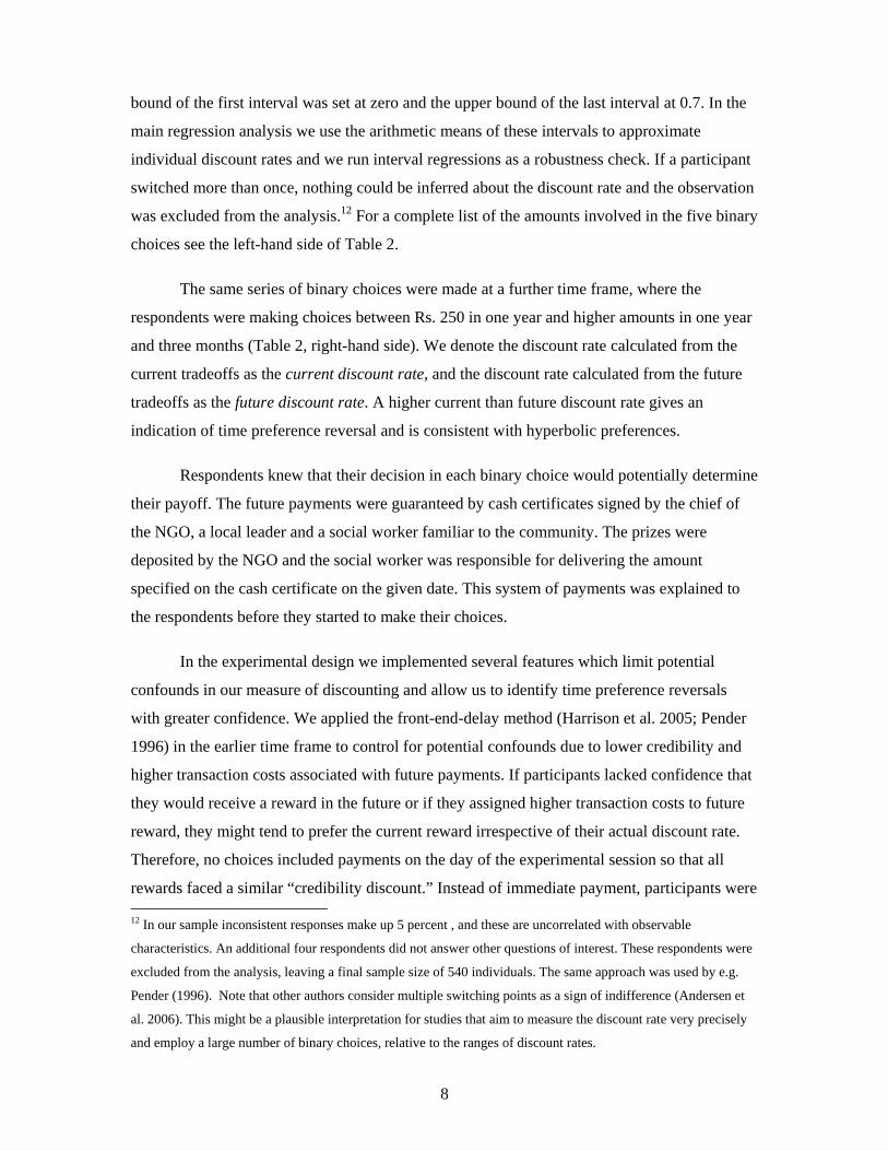
bound of the first interval was set at zero and the upper bound of the last interval at 0.7. In the

main regression analysis we use the arithmetic means of these intervals to approximate

individual discount rates and we run interval regressions as a robustness check. If a participant

switched more than once, nothing could be inferred about the discount rate and the observation

was excluded from the analysis.12 For a complete list of the amounts involved in the five binary

choices see the left-hand side of Table 2.

The same series of binary choices were made at a further time frame, where the

respondents were making choices between Rs. 250 in one year and higher amounts in one year

and three months (Table 2, right-hand side). We denote the discount rate calculated from the

current tradeoffs as the current discount rate, and the discount rate calculated from the future

tradeoffs as the future discount rate. A higher current than future discount rate gives an

indication of time preference reversal and is consistent with hyperbolic preferences.

Respondents knew that their decision in each binary choice would potentially determine

their payoff. The future payments were guaranteed by cash certificates signed by the chief of

the NGO, a local leader and a social worker familiar to the community. The prizes were

deposited by the NGO and the social worker was responsible for delivering the amount

specified on the cash certificate on the given date. This system of payments was explained to

the respondents before they started to make their choices.

In the experimental design we implemented several features which limit potential

confounds in our measure of discounting and allow us to identify time preference reversals

with greater confidence. We applied the front-end-delay method (Harrison et al. 2005; Pender

1996) in the earlier time frame to control for potential confounds due to lower credibility and

higher transaction costs associated with future payments. If participants lacked confidence that

they would receive a reward in the future or if they assigned higher transaction costs to future

reward, they might tend to prefer the current reward irrespective of their actual discount rate.

Therefore, no choices included payments on the day of the experimental session so that all

rewards faced a similar “credibility discount.” Instead of immediate payment, participants were 12 In our sample inconsistent responses make up 5 percent , and these are uncorrelated with observable

characteristics. An additional four respondents did not answer other questions of interest. These respondents were

excluded from the analysis, leaving a final sample size of 540 individuals. The same approach was used by e.g.

Pender (1996). Note that other authors consider multiple switching points as a sign of indifference (Andersen et

al. 2006). This might be a plausible interpretation for studies that aim to measure the discount rate very precisely

and employ a large number of binary choices, relative to the ranges of discount rates.

9

making choices between Rs. 250 delivered the next day and a higher amount delivered in three

months. In order to test for the potential role of lack of trust we also included a question on

trust from the General Social Survey (GSS) into our survey instrument.13 This measure of trust

is not significantly correlated with discount rates or with time preference reversal. The shift

between the current and future time frame was set to one year to avoid the possibility of

confounding factors for time preference reversals due to the seasonality of agricultural incomes

or the regularity of local celebrations.

Histograms in Figure 1 show the distribution of respondents’ choices in the current

(upper graph) and future (lower graph) time frame. The first bar depicts the fraction of

respondents who began by preferring delayed payment in the first binary choice, while the last

bar depicts the fraction of respondents who never switched and preferred the early payment in

all five binary choices. The histograms show that there is substantial heterogeneity in

respondents’ choices. There are two spikes in the first and last bar reflecting respondents who

preferred either earlier or delayed payment in all binary choices. In line with other studies that

elicit discounting in the field in developing countries, the implied discount rates are relatively

high. The three-month current discount rate is on average 24.4 percent and the future discount

rate is 19.2 percent. It is also reassuring to find that our measures of patience intuitively

correlate with saving behavior outside of the lab. Table A.1 in the Appendix shows higher

patience to predict higher savings, the higher likelihood of participation in self-help groups

(local microfinance organizations), and the higher likelihood of having a future-oriented

purpose for savings.

To elicit aversion to risk we used a close replication of the simple protocol designed by

Binswanger (1980) for peasants in ICRISAT villages and later used by e.g. Barr and Genicot

(2008) in Zimbabwe and Nielsen (2001) in Madagascar. Each participant was asked to select

one of six different lotteries. Each lottery yielded either a high or a low payoff with a

probability of 0.5. In each subsequent lottery the expected value increased jointly with the

variance, allowing us to assign a degree of risk aversion. Two sets of prizes were used. The

first one was set at the level of amounts studied in the discount rate questions. The expected

value of the least risky lottery was Rs. 250 and the higher payoff in the most risky lottery was

Rs. 1,000. The second set of prizes was lower, with the expected value of Rs. 30 for the least

13 The wording of the question is: Generally speaking, would you say that most people can be trusted or that you

can’t be too careful in dealing with people?

10

risky lottery and with the maximum payoff of Rs. 120 in the most risky lottery. For a complete

list of amounts involved in the risk aversion experiment see Table 3. To visualize the concept

of equal probabilities, the experimenter simulated how the lottery would work by tossing one

of two numbered ping-pong balls from a bag. Several bags with ping-pong balls were

circulated among the respondents who could attempt this procedure. Payments from lotteries

were disbursed immediately after each research meeting.

Histograms in Figure 2 show the distribution of respondents’ choices of lotteries

involving higher (upper graph) and lower (lower graph) amounts. The first bar depicts the

fraction of respondents who chose the least risky lottery, the last bar represents the fraction of

respondents who chose the most risky lottery. Similarly, as in the case of time discounting

choices, there is substantial heterogeneity in the respondents’ choices. The average degree of

the level of risk aversion in our sample is roughly comparable to other studies that used the

same type of experimental protocol. While the average measure of risk aversion14 in our

sample is 0.4, Binswanger (1981) found this coefficient to range from 0.33 for lotteries

involving low amounts to 0.54 for lotteries involving high amounts and Nielsen (2001) in

Madagascar found it to be 0.32 on average.

III. Results

We start the empirical analysis by looking at gender differences in time discounting and

attitude toward risk. Table 4 presents the regression analysis in which we control only for sex

and age, the exogenous variables. The dependent variable in Columns 1-2 is the current

discount rate. A higher discount rate indicates the more impatient choice. We find that women

made more patient choices than men: the three-month current discount rate is 5.1 percentage

points lower for women (Column 1). This difference is statistically significant (1% level) and

relatively large in size; the mean current discount rate of the whole sample is 24.4 percent. The

dependent variable in Columns 3 and 4 is the future discount rate. The gender difference in the

future discount rate is even larger (Column 3).

14 The measure of risk aversion assigned to each lottery is approximated by the average of an interval with a

lower bound given by (Ex+1-Ex)/(SEx+1-SEx) and upper bound given by (Ex-Ex-1)/(SEx-SEx-1), where Ex is the

expected value and SEx is the standard deviation of the lottery; Ex-1 and SEx-1 are values for the lottery one row

above and Ex+1 and SEx+1 for the lottery one row below. The upper bound for the first lottery is set to one and the

lower bound for the last lottery is set to zero.

11

The dependent variable in Columns 5 and 6 is equal to one if an individual makes a

more impatient choice in the current time frame than in the future time frame. We test whether

we identify gender differences in the likelihood of time preference reversal and we do not find

any.

In Columns 7-10 we focus on choices among lotteries with different levels of risk

(Table 4). The dependent variable has six values. We did not impose any particular structure on

the individual utility function to derive an index of risk aversion. We labeled the lotteries from

1 to 6, where 6 is the most risky gamble. For lotteries with lower stakes we find that women

are more risk averse, although the difference is only marginally significant statistically

(Column 9). For higher stakes, the relationship is weaker (Column 7).

These results are robust to controlling for village fixed effects (Columns 2, 4, 6, 8, 10

of Table 4) and alternative estimation techniques (Table A.2 in the Appendix). In Columns 1-4

of Table A.2 we show that results on discount rates are similar if we use interval regressions

instead of OLS to account for the fact that the dependent variables are measured in intervals,

and that all observations are right and left censored. In Columns 5-8 of Table A.2, where the

dependent variables are the chosen lotteries, we use ordered probit instead of OLS.

In further empirical analysis we explore the potential reasons for the higher patience of

women. In doing so, we focus on the number of children below 18 years old, i.e. those that

they have to take care of. The average number of children below 18 years in our sample is 1.8

and Figure 3 shows the histogram. We start this analysis by looking at this relationship in the

raw data. In the upper part of Figure 4 we observe that women without any children below 18

years of age have an average current discount rate of 25.1 percent, with one child it is 20.3

percent and reaches a minimum with four children (red line). As indicated by 95 percent

confidence intervals, women with three or four children are significantly more patient than

women with no children. Hence, there seems to be a clear pattern between more children and

the higher patience of women. Note that this pattern holds over the range of children (up to

four) that is most common in our sample (see Figure 3). There are only eleven women who

have more than four children below 18 years old (Figure 4), as indicated by large confidence

intervals, and these women made very impatient choices.

There seems to be no similar relationship for men (the blue line in Figure 4). It is

interesting to note small differences in the discount rates between men and women who do not

have young children. With more children, the discount rates start to diverge as women’s

12

patience increases. When having three or four young children, the difference between men’s

and women’s discount rate is more than 10 percentage points and is significant at 5% (the

green line in Figure 4). These patterns are similar for the future discount rate (lower part of

Figure 4). Thus, the figures provide an initial indication for two interesting patterns: the

increasing patience of women with up to four children and gender differences in patience that

linearly increase with more children.

In order to assess how statistically significant these relationships are and whether they

are robust to controlling for observable characteristics, we next regress our measures of

patience on the number of children and its square, and on various controls. Table 5 presents the

results, in Panel A the dependent variable is the current discount rate and in Panel B it is the

future discount rate. In Column 2 of Panel A we restrict the sample to only women and find

strong evidence for a u-shaped relationship between their current discount rate and the number

of children, with the highest level of patience associated with approximately three children

below 18 years old. In Column 2 of Panel B we find that women with more children have a

lower future discount rate, similarly as in the case of the current discount rate. Nevertheless,

the evidence for the u-shaped pattern, in particular the upward sloping area, is statistically less

significant for the future discount rate. This slight difference is plausible. It is very unusual to

have more than four children, and inter-temporal choices in the current time frame are more

likely to be affected by the current needs of an extremely large family than the same choices in

the future time frame.

To study whether the number of children is predictive for gender heterogeneity in

preferences, we run the regressions for the whole sample and interact the number of children

with a dummy for being a female (Columns 1 and 4 of Table 5). We find that each additional

child is associated with a 1.4-2.9 percent reduction in the women’s discount rate relative to

men’s, depending on the specification. The separate dummy for being a female no longer

predicts more patient choices, in contrast to results in Table 4. We obtain very similar results

when we use interval regression as an alternative estimation technique (Table A.3 in the

Appendix).

Overall, the baseline result suggests a greater willingness to make patient choices

among women that have a higher number of children over the range of children that are usual

for Indian families (up to four children below 18 years old). Since we do not observe the same

pattern for men, the higher number of children also predicts the higher patience of women

13

compared to men. This is also true when controlling for village fixed effects and using an

alternative estimation strategy. In the following sub-sections we use rich survey data about our

participants and do a series of robustness checks to rule out various alternative explanations for

the apparent link between the number of children and women’s patience.

IV. Robustness Checks

The baseline result could potentially be due to other variables. Table 6 presents the same

regressions as in Table 5, but adding other, potentially endogenous, observable variables. In

Panel A the dependent variable is the current discount rate and in Panel B it is the future

discount rate.

First we explore whether the results are robust to controlling for education. Following

Becker and Mulligan (1997) it is often hypothesized that education can affect time preference,

because schooling may promote the creation of cognitive skills, the ability to simulate and plan

for the future (McClure et al. 2004). Several studies have found a strong correlation between

education and discounting (see, e.g., Harrison et al. 2002; Kirby et al. 2002) or cognitive skills

and discounting (Sunde et al. forthcoming). Recently, Bauer and Chytilová (forthcoming)

found evidence for the causal effect of education on lower time discounting in Uganda. At the

same time there is a large body of evidence based on the World Fertility Surveys and

Demographic and Health Surveys that establishes a strong association between education and

fertility across developing countries (e.g. Weinberger 1987; Martin 1995). However, it is found

that people with higher education have a lower number of children, a pattern with the opposite

sign to explain the children-discounting correlation in our sample.

In line with the reasoning above, we observe that individuals with more years of

schooling make more patient choices.15 Importantly for the main pattern of interest, we see that

the baseline link between children and women’s patience is largely unchanged by controlling

for education (Column 2 of Table 6). The interaction term showing the gender heterogeneity in

patience to be associated with the number of children is smaller for the current discount rate

(and only marginally significant), the coefficient for the future discount rate is very similar and

significant (Column 1 of Table 6).

15 The full results of Table 6, including the correlations with education and other observable characteristics, are available in the Web Appendix [to be included].

14

Second, discounting may be a function of income or credit constraints (Pender 1996).

Since it is not entirely clear in which direction wealth or income constraints may affect fertility

on an individual level, it is desirable to test if the baseline results hold when we add wealth and

self-reported information on the seasonality of income in our regressions (Columns 3, 4 of

Table 6). To approximate wealth we calculated an index by principal component analysis from

questions on the type of house, electricity connection, land ownership and dummies for the

possession of 14 types of household equipment. To identify individuals who have a relatively

low income at the time of the experiment relative to three months later we asked the

participants what months are their high-income and low-income months.

We find the intuitive result that wealthier individuals make more patient choices.16 A

higher relative income at the time of the experiment does not emerge as a significant predictor

of discounting. Importantly, the link between children and women’s patience is unaffected by

controlling for these variables for both the current and future discount rate.

A third possible explanation, in particular for gender heterogeneity in the level of the

discount rates, could be related to different outside opportunities faced by men and women. If

men intended to use the experimental rewards for a profitable investment and women with

young children were less likely to do so, then women might opt for choices that make them

look more patient. Contrary to this argument, our findings show that impatient men are more

likely to save for consumption rather than for investment purposes (Table A.1). Furthermore, if

certain social norms prevented women from undertaking a profitable investment we would

expect women with a stronger intra-household position to make more impatient choices in our

experiment. We measure the women’s position by an index calculated by principal component

analysis from seven questions on decision-making and five questions on wife-beating these

questions are commonly used in Demographic and Health Surveys. In addition, we control for

being married and being the head of a household. In Column 5 of Table 6 we show that the

baseline result is robust to these measures.17

16 The discounting-wealth correlation vanishes when we control for education (not reported, available upon

request). This is consistent either with the more important role of education as a determinant of patience or with

the fact that education is typically measured more precisely than wealth. 17 The module on the intra-household position is relevant only for women. Thus, we report the results only for

women (Column 5 of Table 6).

15

Fourth, since the number of children is tied to different stages of life, the effect of

children might be overestimated if it captured unobserved life cycle effects. For example,

Becker and Mulligan (1997) predict a u-shaped relationship between age and patience due to

the effects of learning to be future-oriented during youth and the recognition of a shortening

life expectancy during aging. If the first effect overlapped with children being born and the

second one with children becoming adults, we could also observe a positive correlation

between the number of young children and patience. In all regressions we control for age. In

addition, we do not observe a statistically significant relationship between age and discount

rate even if we do not control for the number of children (Table 4). Thus, age effects should not

drive our baseline results.

So far we have assumed the utility function to be locally linear for the stakes used in the

inter-temporal choice experiments. As discussed in Andersen et al. (2008), with the higher

concavity of utility function a lower discount rate is needed to generate the same degree of

impatience in inter-temporal choices. In line with the recent contributions of Andersen et al.

(2008) or Tanaka et al. (forthcoming), we have jointly elicited measures of the discount rate

and risk aversion, the latter of which can be, under certain assumptions, used as a proxy for the

concavity of the utility function.

As a fifth robustness check we investigate whether the result that women with more

children are more patient indicates a direct link between children and time preference, or

whether it could be driven by a possibility that women with children have a less concave utility

function (i.e., are less risk averse). One possibility to control for risk aversion is to make a

strong assumption about the form of utility function, estimate parameters describing curvature

(e.g., CRRA) and then estimate the discount rate implied by inter-temporal choices (as in

Andersen et al. 2008). Another way, which we apply in this paper and which circumvents the

need to make assumptions about the form of utility function, is to control directly for observed

risk attitudes. We allow risk attitudes to enter the regression non-parametrically, with a dummy

for each lottery chosen in the risk experiment (as in Sunde et al. forthcoming).

Columns 6 and 7 of Table 6 present the results. For the current discount rate we find the

same baseline relationships between children and women’s patience. For the future discount

rate the relationship is slightly less statistically significant. These results suggest that the

observed relationship between children and patient choices is primarily driven by pure time

preference rather than the curvature of the utility function. In Columns 8 and 9 we add all the

16

observable characteristics and village fixed effects into the regression. Controlling for all of

this the main patterns still survives.

In the previous estimation we study the children-patience relationship by including the

number of children below 18 years old and its squared term. Table A.4 in the Appendix is

ambitious given the sample size as it includes dummy variables for each number of children to

estimate non-parametrically the relationship between patience and the number of children. The

omitted variable is having no children. This estimation directly supports previous observations,

where for women who have three or four children we observe significantly lower discount rates

(Columns 2,4,6,8). The interaction terms of being a female and having different numbers of

children generally supports the hypothesis that gender heterogeneity in preferences increases

with the number of children (Columns 1,3,5,7), although they are not always statistically

significant.

Taken together, the picture emerging from the results in this section is that there is a

relationship between the number of children and women’s patience, which is unlikely to be

driven by other observable individual characteristics such as age, education, wealth, decision-

making power, risk aversion, or by village level characteristics. In the next section we explore

this pattern further by looking at whether and how the age and sex composition of children is

predictive of women’s patience. This analysis allows us to make tentative statements regarding

the underlying causal direction of the observed relationship.

V. Composition of Children and Patience

Let us consider why a woman with young children makes more patient inter-temporal choices.

Very intuitively, being a parent may influence how people think about future. The more

children the more patience effect is predicted, for example, by the model of backward

discounting with dual selves (Ray and Wang 2001), one of them being a child, as discussed

earlier. The causal effect of children on patience is also consistent with a situation when

parents need to save for a certain high return investment opportunity that is available

specifically to children, such as education, or with a need to create more precautionary savings

if children are in the family. In this context it is not very surprising that we observe the

children-patience relationship specifically for women, as there are countless evolutionary or

anthropological studies emphasizing the closer attachment of women to their children

compared to men.

17

Alternatively, there may be a causal effect in the opposite direction; being patient may

affect the number of children one would prefer to have. Following the traditional assumption of

Becker and Tomes (1976) about altruistic parents, one could argue that more patient parents

put a greater weight on the quality of their children in the form of investment in their human

capital. Since higher quality children are costly, more patient parents would prefer to have

fewer children. However, this reasoning implies the opposite of the relationship that we

observe. Nevertheless, parents might consider children as a form of investment in providing

better care for their old age. In this case, patient individuals would want more children, which

is a consistent prediction with our results.

Although we do not have an exogenous source of variation in fertility to test a causal

effect on women’s patience directly, we believe our results suggest that the greater women’s

patience with a higher number of children is not driven by patience causing a higher number of

children. To study these questions we explore the information about age and sex composition

of children of our respondents. If children were an investment for old age we should observe a

closer connection between patience and the total number of children than between patience and

young children. In other words, the age composition of children should not play an important

role in the estimates. On the other hand, if women become more patient with children they are

responsible for, we would expect important differences in the association with children of a

different age. In particular non-adult children, those that the mother must take care of, should

be more important than children who have already reached the adult age.

In Table 7 the dependent variables are again the current discount rate (Columns 1-3)

and the future discount rate (Column 4-6). The sample is restricted to women and we control

for all the observable characteristics and village fixed effects. In Columns 1 and 4 the

explanatory variables are the number of children that are younger than 18 years, the total

number of children including those that are already adults, and their squared terms. The

estimated coefficient for the children below 18 then indicates how the discount rate changes

with more children below 18, keeping the total number of children constant. In other words, it

estimates the effect of increasing the proportion of children below 18. We observe sharp

differences depending on the age of the children. We see the same u-shaped relationship

between discount rates and children below 18 years old, keeping the total number of children

constant. The lowest discount rate is again associated with 3-3.5 children below 18 years old.

For the current discount rate this relationship is significant at a 1% level, for the future discount

18

rate it is only marginally significant. Having a higher total number of children, while keeping

the number of children below the age of 18 constant, does not affect patience.

In Columns 2 and 5 of Table 7 we go one step further in categorizing children into

different age groups. We are interested in exploring the question of whether it is only very

small children (below 5 years old) that make women more patient (up to a point), or if it is

school-aged children (5-18 years old), or in general all children that a women has to take care

of (all below 18 years old). In the regression, the explanatory variables remain the total number

of children and the number of children below 18 years of age, and we add the number of

children below 5 years of age. Now the coefficient for the number of children below 5 years

old indicates the change in the discount rate if the proportion of children below 5 years old

among children below 18 years old increases. For the current discount rate (Column 2) we

observe no significantly different effect for having very small children compared to other

children below 18 years old. The coefficients for the number of children below 18 years old,

which tell us the effect of having more children in the age range of 5-18 years at the expense of

children older than 18 years old, remain statistically significant. For the future discount rate

(Column 5) we see a somewhat stronger correlation for very small children relative to other

children below 18 years old, although with quite a lot of uncertainty.

Overall, it seems that the link between the number of children and women’s patience is

particular for the children that she has to look after. The intensity of interaction and

responsibility for those children seems to enter women’s inter-temporal optimization and these

results are thus more consistent with the causal effect of having children on women’s patience.

Within the group of children below 18 years old we do not find big differences between the

children who are very small (below 5 years old) and those who are older (5-18 years old).

Another important question is whether women’s inter-temporal optimization is more

affected by having sons than by having daughters, or if the pattern is related to having children

in general. In the context of India and other developing countries this question is particularly

relevant. For example, the dowry system may motivate parents to be more patient after having

a daughter. Deolalikar and Rose (1998) show the positive impact of a daughter relative to a son

on household savings. There is also substantial empirical literature on sibling rivalry that

shows that parents tend to discriminate against daughters and invest more in their sons in terms

of education and health (Morduch 2000; Ota and Moffatt 2006).

19

In Columns 3 and 6 of Table 7 the explanatory variables of interest are children below

18 years of age, sons below 18 years and their squared terms. We do not find that higher

proportion of sons on children below 18 would predict the more patient choices of women, in

both the current and future time frame. We still find that the number of children below 18 in

general predicts patience with statistical significance. Thus, the relationship with patience

seems to be independent of the gender of the children and hence unlikely to be driven solely by

dowry considerations or higher returns to the human capital of sons. Tentatively, it seems more

consistent with a notion that women’s inter-temporal optimization is affected by having

responsibility for children in general.

VI. Conclusions

The main goal of this paper was to investigate whether more future-oriented behavior among

women in developing countries can be linked to direct measures of preferences and whether the

key traits of patience and risk aversion are systematically related to the number of their

children. In order to test this hypothesis, we used a large random sample of individuals living

in rural India, incentive compatible measures of patience and risk aversion, and detailed survey

data on economic and family characteristics.

We found women to make more patient choices than men on average. Most

interestingly, we found increasingly patient choices among women who had higher number of

children below 18 years of age, with the highest level of patience being associated with three to

four children. We observe important differences in this link, depending on the age of the

children. Women’s patience is correlated only with children who are younger than 18 years old

― and hence those she has to look after ― but not with children that are already adults. We do

not find a link between children and men’s patience. Thus, a higher number of children also

predicts the significantly higher patience of women compared to men. The relationships hold

also after controlling for education, wealth and other personal characteristics, village fixed

effects, and are robust to alternative estimation techniques.

Our results have several important implications. They are consistent with the view that

empowering women in developing countries is likely to be associated with increased levels of

savings and investments, which are, in turn, likely to contribute to future growth (Rubalcava et

al. 2007). The results may also inform the growing literature that studies intra-household

decision-making (for a survey see Xu 2007), because the findings do not concur with one of

20

the key assumptions of the Beckerian unitary household model: homogeneity of preferences.

Furthermore, the findings suggest conditions under which this assumption is less likely to hold

and thus, spouses’ conflicting spending preferences are more likely to emerge. For example,

Anderson and Baland (2002) show that married women are more likely to participate in

rotating saving and credit associations (ROSCAs). They argue that women use the group

commitment to save as a way to protect their savings against their husband’s claims for

immediate consumption. Our findings suggest that strategies that aim to discipline divergent

preferences of the spouses may be correlated with the responsibility of women to take care of

their children. Lastly, understanding the determinants of individual time discounting and

attitude to risk is one of the central topics in economics and psychology. Existing experimental

studies conducted in the field pay particular attention to economic factors such as education,

wealth and liquidity constraints. Our results suggest that the responsibility for their children’s

future can shape women’s patience, and thus the intra-family context should be taken seriously

in studying their preferences.

There are several specific mechanisms as to why children can be associated with higher

patience. Ray and Wang (2001) argue that parents may imprint the future of their child in their

discount function as a future self. The more the parents interact with their children the lower

the discount rate should be. Their model implies that the link with children is more likely to be

seen in societies in which parents spend most of their time at home surrounded by their

children. Second, children might be viewed as a way to invest in the future. If returns to

investments in the quality of children (such as education) are high, then parents with children

are more motivated to save for these investments, and hence put a lower weight on current

consumption. This reasoning implies that the link between children and patience should be

more apparent in societies with high returns to child-specific investments. Third, having

children makes a family more vulnerable to unexpected shocks, due to both additional health

risks and due to the larger effects of income fluctuations. Parental responsibility for the

survival of children could strengthen the need to build up a buffer of precautionary savings.

Thus, the observed link between children and patience might be more profound in societies

with high uncertainty and worse access to insurance mechanisms. Lastly, more patient

individuals may prefer to have a higher quantity of children, although this hypothesis is not

consistent with our more detailed analysis on the age composition of children and patience.

Investigating these alternative mechanisms further is an open question for future research.

21

REFERENCES

Anderson, Siwan, and Jean-Marie Baland (2002). “The Economics of ROSCAs and

Intrahousehold Resource Allocation.” Quarterly Journal of Economics, 117(3), 963–995.

Andersen, Steffen, Glenn W. Harrison, Morten I. Lau, and E. Elisabet Rutström (2008).

“Eliciting Risk and Time Preferences.” Econometrica, 76(3), 583–618.

Ashraf, Nava, Dean Karlan, and Wesley Yin (2006). “Tying Odysseus to the Mast: Evidence

from a Commitment Savings Product in the Philippines.” Quarterly Journal of Economics,

121(2), 635–672.

Barr, Abigail, and Garance Genicot (2008). “Risk Sharing, Committment and Information: An

Experimental Analysis ” Journal of the European Economic Association, 6(6), 1151–1185.

Bauer, Michal, and Julie Chytilová (forthcoming). “The Impact of Education on Subjective

Discount Rate in Ugandan Villages.” Forthcoming in Economic Development and Cultural

Change.

Becker, Gary S., and Casey B. Mulligan (1997). “The Endogenous Determination of Time

Preference.” Quarterly Journal of Economics, 112(3), 729–758.

Becker, Gary S., and Nigel Tomes (1976). “Child Endowments and the Quantity and Quality

of Children.” Journal of Political Economy, 84(4), S143–S162.

Binswanger, Hans P. (1980). “Attitudes toward Risk: Experimental Measurement in Rural

India.” American Journal of Agricultural Economics, 62, 395–407.

Cardenas, Juan Camilo, and Jeffrey P. Carpenter (2008). “Behavioural Development

Economics: Lessons from Field Labs in the Developing World.” Journal of Development

Studies, 44(3), 311–338.

Croson, Rachel, and Uri Gneezy (forthcoming). “Gender Differences in Preferences.”

Forthcoming in Journal of Economic Literature.

Deolalikar, Anil, and Elaina Rose (1998). “Gender and Savings in Rural India.” Journal of

Population Economics, 11(4), 453–470.

Doepke, Matthias, and Michele Tertilt (forthcoming). “Women’s Liberation: What’s in it

forMen?” Forthcoming in Quarterly Journal of Economics, 124(4).

22

Duflo, Esther (2003). “Grandmothers and Granddaughters: Old-Age Pensions and

Intrahousehold Allocation in South Africa.” World Bank Economic Review, 17, 1–25.

Eckel, Catherine C., and Philip J. Grossmann (2006a). “Men, Women and Risk Aversion:

Experimental Evidence.” In Plott, Charles, and Vernon Smith (eds.), Handbook of

Experimental Economics Results. Elsevier: New York.

Eckel, Catherine.C., and Philips J. Grossmann (2006b). “Differences in Economic Decisions of

Men and Women: Experimental Evidence. ” In Plott, Charles, and Vernon Smith (eds.),

Handbook of Experimental Economics Results. Elsevier: New York.

Edlund, Lena, and Nils-Petter Lagerlof (2004). “Implications of Marriage Institutions for

Redistribution and Growth. ” Unpublished manuscript, Columbia University.

Frederick, Shane, George Loewenstein, and Ted O'Donoghue (2002). “Time Discounting and

Time Preference: A Critical Review.” Journal of Economic Literature, 40(2), 351–401.

Harrison, Glenn W., Morten Igel Lau, Elisabet E. Rutström, and Melonie B. Sullivan (2005).

“Eliciting Risk and Time Preferences Using Field Experiments: Some Methodological Issues.”

In Carpenter, Jeffrey, Glenn W. Harrison, and John A. List (eds.), Field Experiments in

Economics. Greenwich.

Harrison, Glenn W., Morten Igel Lau, and Melonie B. Williams (2002). “Estimating Individual

Discount Rates in Denmark: A Field Experiment.” American Economic Review, 92(5), 1606–

1617.

Kirby, Kris N., and N. Marakovic (1996). “Delay-Discounting Probabilistic Rewards: Rates

Decrease as Amounts Increase.” Psychonomic Bulletin and Review, 3, 100–104.

Kirby, Kris .N., Ricardo Godoy, Victoria Reyes-García, Elizabeth Byron, Lilian Apaza,

William Leonard, Eddy Pérez, Vincent Vadez, and David Wilkie (2002). “Correlates of

Delay-Discount Rates: Evidence from Tsimane’ Amerindians of the Bolivian Rain Forest.”

Journal of Economic Psychology, 23(3), 291–316.

Martín, Teresa Castro (1995). “Women’s Education and Fertility: Results from 26

Demographic and Health Surveys.” Studies in Family Planning, 26(4), 187–202.

23

McClure, Samuel M., David I. Laibson, George Loewenstein, Jonathan D. Cohen (2004).

“Separate Neural Systems Value Immediate and Delayed Monetary Rewards.” Science, 306,

503–507.

Miller, Grant (2008). “Women’s Suffrage, Political Responsiveness, and Child Survival in

American History.” Quarterly Journal of Economics, 123(3), 1287–1327.

Morduch, Jonathan (2000). “Siblings Rivalry in Africa.” American Economic Review, 90(2),

405–409.

Nielsen, Uffe (2001). “Poverty and Attitudes Towards Time and Risk: Experimental Evidence

from Madagascar.” Royal Veterinary and Agricultural University of Denmark Working Paper.

Ota, Masako, and Peter G. Moffatt (2006). “The Within-Household Schooling Decision: A

Study of Children in Rural Andhra Pradesh.” Journal of Population Economics, 20(1), 223–

239.

Pender, John L. (1996). “Discount Rates and Credit Markets: Theory and Evidence from Rural

India.” Journal of Development Economics, 50(2), 257–296.

Ray, Debraj, and Ruqu Wang (2001). “On Some Implications of Backward Discounting.”

Unpublished manuscript.

Rubalcava, Luis, Graciela Teruel, and Duncan Thomas (2009). “Investments, Time Preferences

and Public Transfers Paid to Women.” Economic Development and Cultural Change, 57(3),

507–538.

Silverman, Irwin W. (2003). “Gender Differences in Delay of Gratification: A Meta-Analysis.”

Sex Roles, 49, 452–463.

Sunde, Uwe, Thomas Dohmen, Armin Falk, and David Huffman (forthcoming). “Are Risk

Aversion and Impatience Related to Cognitive Ability?” Forthcoming in American Economic

Review.

Tanaka, Tomomi, Colin Camerer, and Quang Nguyen (forthcoming). “Risk and Time

Preferences: Experimental and Household Data from Vietnam.” Forthcoming in American

Economic Review.

Thomas, Duncan (1990). “Intra-Household Resource Allocation: An Inferential Approach.”

Journal of Human Resources, 25(4), 635–664.

24

United Nations Population Division, Department of Economic and Social Affairs (2005).

Guidelines on Women’s Empowerment.The United Nations: New York, NY.

Weinberger, Mary Beth (1987). “The Relationship Between Women’s Education and Fertility:

Selected Findings from the World Fertility Surveys. ” International Family Planning

Perspectives, 13(2), 35–46.

Xu, Zeyu (2007). “A Survey on Intra-Household Models and Evidence.” University Library of

Munich, MPRA paper 3763.

Yunus, Muhammad (2002). “Toward Eliminating Poverty from the World: Grameen Bank

Experience.” In Anderson, C. Leigh, and Janet W. Looney (eds.), Making Progress: Essays in

Progress and Public Policy. Lanham.

25

FIGURES AND TABLES

Figure 1: Distribution of choices in inter-temporal choice experiments

0.1

.2.3

.4.5

Frac

tion

1 2 3 4 5 6Switching row in the future time frame

0.1

.2.3

.4.5

Frac

tion

1 2 3 4 5 6Switching row in the current time frame

26

Figure 2: Distribution of choices in the lotteries

Figure 3: Distribution of children below 18 years of age

0.1

.2.3

.4Fr

actio

n

0 2 4 6 8Children below 18 years

0.1

.2.3

Frac

tion

1 2 3 4 5 6Chosen lottery (lower amounts)

0.1

.2.3

Frac

tion

1 2 3 4 5 6Chosen lottery (higher amounts)

27

Figure 4: Discount rates and number of children younger than 18 years of age

-.4-.2

0.2

.4.6

Futu

re d

isco

unt r

ate

0 1 2 3 4 >4Number of children

MaleFemaleDifference btw . Female and Male

-.4-.

20

.2.4

.6C

urre

nt d

isco

unt r

ate

0 1 2 3 4 >4Number of children

MaleFemaleDif f erence btw. Female and Male

Table 1: Sample characteristics, comparison with Karnataka averages (means and standard deviations)

Total Female Male Honavar Haliyal Karnatakaa

Age (years) 36.869 35.537 38.180 36.852 36.885 36.300 (11.740) (11.273) (12.061) (11.015) (12.443) Education (classes) 4.244 3.485 4.993 5.970 2.519 4.200 (4.433) (4.041) (4.675) (4.474) (3.658) Illiterate 0.396 0.451 0.342 0.204 0.589 0.425 (0.490) (0.499) (0.475) (0.403) (0.493) Married 0.789 0.780 0.798 0.733 0.844 0.670 (0.408) (0.415) (0.402) (0.443) (0.363) Farmer 0.703 0.669 0.737 0.643 0.772 0.750b (0.457) (0.471) (0.441) (0.483) (0.420) Sample size 540 268 272 270 270

Notes: Standard deviations in parentheses. a Source: Indian Census 2001: data for the Karnataka population above 15 b Only the rural population in Karnataka

Table 2: Payoff table (discount rates)

Binary choices in the current time frame Binary choices in the future time frame

Tomorrow After three months After one

year After one year and

three months Choice 1 Rs. 250 Rs. 265 Choice 1 Rs. 250 Rs. 265 Choice 2 Rs. 250 Rs. 280 Choice 2 Rs. 250 Rs. 280 Choice 3 Rs. 250 Rs. 300 Choice 3 Rs. 250 Rs. 300 Choice 4 Rs. 250 Rs.330 Choice 4 Rs. 250 Rs.330 Choice 5 Rs. 250 Rs. 375 Choice 5 Rs. 250 Rs. 375

29

Table 3: Payoff table (attitude to risk)

Attitude to risk (high amounts) Attitude to risk (low amounts)

Lottery Bad luck payoff

(50%) Good luck payoff

(50%) Lottery Bad luck

payoff (50%) Good luck payoff

(50%) 1 Rs. 250 Rs. 250 1 Rs. 30 Rs. 30 2 Rs. 225 Rs. 475 2 Rs. 27 Rs. 57 3 Rs. 200 Rs. 600 3 Rs. 24 Rs. 72 4 Rs. 150 Rs. 750 4 Rs. 18 Rs. 90 5 Rs. 50 Rs. 950 5 Rs. 6 Rs. 114 6 Rs. 0 Rs. 1000 6 Rs. 0 Rs. 120

Table 4: Gender heterogeneity in preferences

Estimator OLS OLS Probit OLS OLS Dependent variable: Current discount rate Future discount rate Hyperbolic

Risk aversion (high amounts)

Risk aversion (low amounts)

(1) (2) (3) (4) (5) (6) (7) (8) (9) (10) Female -0.051 -0.042 -0.066 -0.061 0.036 0.046 -0.107 -0.121 -0.181 -0.225 (0.020)*** (0.019)** (0.019)*** (0.019)*** (0.041) (0.042) (0.134) (0.132) (0.134) (0.134)* Age -0.005 -0.000 -0.002 0.002 -0.000 -0.002 -0.009 -0.027 0.002 -0.015 (0.005) (0.004) (0.004) (0.004) (0.009) (0.010) (0.031) (0.031) (0.031) (0.032) (Age)2 0.000 0.000 0.000 -0.000 0.000 0.000 0.000 0.000 -0.000 0.000 (0.000) (0.000) (0.000) (0.000) (0.000) (0.000) (0.000) (0.000) (0.000) (0.000) Constant 0.335 0.165 0.262 0.133 4.049 4.585 4.092 5.037 (0.086)*** (0.096)* (0.084)*** (0.095) (0.591)*** (0.671)*** (0.592)*** (0.681)***Village fixed effects? no yes no yes no yes no yes no yes Observations 540 540 540 540 540 540 540 540 540 540 (Pseudo) R-squared 0.02 0.15 0.02 0.11 0.01 0.03 0.00 0.09 0.01 0.07

30

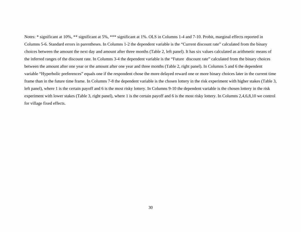
Notes: * significant at 10%, ** significant at 5%, *** significant at 1%. OLS in Columns 1-4 and 7-10. Probit, marginal effects reported in

Columns 5-6. Standard errors in parentheses. In Columns 1-2 the dependent variable is the “Current discount rate” calculated from the binary

choices between the amount the next day and amount after three months (Table 2, left panel). It has six values calculated as arithmetic means of

the inferred ranges of the discount rate. In Columns 3-4 the dependent variable is the “Future discount rate” calculated from the binary choices

between the amount after one year or the amount after one year and three months (Table 2, right panel). In Columns 5 and 6 the dependent

variable “Hyperbolic preferences” equals one if the respondent chose the more delayed reward one or more binary choices later in the current time

frame than in the future time frame. In Columns 7-8 the dependent variable is the chosen lottery in the risk experiment with higher stakes (Table 3,

left panel), where 1 is the certain payoff and 6 is the most risky lottery. In Columns 9-10 the dependent variable is the chosen lottery in the risk

experiment with lower stakes (Table 3, right panel), where 1 is the certain payoff and 6 is the most risky lottery. In Columns 2,4,6,8,10 we control

for village fixed effects.

Table 5: Children and patience: main results

(1) (2) (3) (4) (5) (6) Sample: All Women Men All Women Men Panel A Dependent variable: Current discount rate Female -0.007 -0.017 (0.029) (0.028) Children below 18 -0.017 -0.072 0.008 -0.031 -0.073 -0.022 (0.019) (0.024)*** (0.029) (0.019)* (0.022)*** (0.029)(Children below 18)2 0.008 0.013 0.004 0.008 0.013 0.006 (0.004)** (0.005)*** (0.006) (0.004)** (0.004)*** (0.006)Female*Children below 18 -0.025 -0.014 (0.012)** (0.012) Village fixed effects? no no no yes yes yes Observations 540 268 272 540 268 272 R-squared 0.04 0.03 0.05 0.16 0.27 0.21 Panel B Dependent variable: Future discount rate Female -0.013 -0.018 (0.028) (0.028) Children below 18 0.008 -0.039 0.027 -0.000 -0.036 0.012 (0.019) (0.022)* (0.029) (0.019) (0.022)* (0.030)(Children below 18)2 0.005 0.007 0.002 0.004 0.006 0.002 (0.004) (0.004) (0.006) (0.004) (0.004) (0.006)Female*Children below 18 -0.029 -0.024 (0.012)** (0.012)** Village fixed effects? no no no yes yes yes Observations 540 268 272 540 268 272 R-squared 0.04 0.01 0.04 0.12 0.18 0.14

Notes: * significant at 10%, ** significant at 5%, *** significant at 1%. OLS, standard errors

in parentheses. In Panel A the “Current discount rate,” in Panel B the dependent variable is the

“Future discount rate.” In all columns we control for age and its squared term. In Columns 4-6

we control for village fixed effects.

Table 6: Children and current patience ― robustness checks

(1) (2) (3) (4) (5) (6) (7) (8) (9) Sample: All Women All Women Women All Women All Women Panel A Dependent variable: Current discount rate Female -0.043 -0.012 -0.008 -0.045 (0.029) (0.029) (0.029) (0.031) Children -0.032 -0.077 -0.028 -0.075 -0.124 -0.016 -0.066 -0.045 -0.089 (0.019)* (0.024)*** (0.019) (0.024)*** (0.028)*** (0.019) (0.024)*** (0.021)** (0.025)***(Children)2 0.009 0.013 0.010 0.013 0.021 0.008 0.011 0.010 0.015 (0.004)** (0.005)*** (0.004)*** (0.005)*** (0.005)*** (0.004)** (0.005)** (0.004)*** (0.005)***Children below 18 * Female -0.019 -0.023 -0.025 -0.014 (0.012) (0.012)* (0.012)** (0.012) Panel B Dependent variable: Future discount rate Female -0.050 -0.019 -0.015 -0.060 (0.028)* (0.028) (0.028) (0.031)** Children -0.007 -0.044 -0.003 -0.043 -0.066 0.010 -0.035 -0.014 -0.046 (0.018) (0.022)** (0.019) (0.023)* (0.026)** (0.019) (0.023) (0.021) (0.025)* (Children)2 0.006 0.007 0.006 0.007 0.011 0.004 0.006 0.006 0.007 (0.003) (0.004)* (0.004) (0.005) (0.005)** (0.004) (0.005) (0.004) (0.005) Children below 18 * Female -0.023 -0.027 -0.030 -0.025 (0.011)** (0.012)** (0.012)** (0.012)** Education? yes yes no no no no no yes yes Wealth, Relative income? no no yes yes no no no yes yes Married, Household head, Position, Position2? no no no no yes no no yes yes Risk aversion dummies? no no no no no yes yes yes yes Age, Age2? yes yes yes yes yes yes yes yes yes Village fixed effects? no no no no no no no yes yes Observations 540 268 540 268 251 540 268 540 268

33

Notes: * significant at 10%, ** significant at 5%, *** significant at 1%. OLS, standard errors in parentheses. In Panel A the dependent variable is

the “Current discount rate,” in Panel B the dependent variable is the “Future discount rate.” “Education” is measured as years of schooling.

“Wealth” is an index calculated by principal component analyses from questions on the type of house, electricity connection, land ownership and

dummies for the possession of 14 types of household equipment. “Relative income” is a dummy equal to one if the individual income is higher in

June (time of the experiment) than in September (timing of delayed payoffs). “Position” is an index calculated for women by principal component

analyses from seven questions on decision making and five questions on wife-beating. The minimum of the index is set to zero; the higher the

index value, the better the position. “Risk aversion” is a set of six dummies corresponding to the chosen lottery.

Table 7: Women, composition of children and patience

(1) (2) (3) (4) (5) (6) Sample: Women Women Women Women Women Women

Dependent variable: Current discount rate Future discount rate Children below 5 -0.035 -0.046 (0.051) (0.050) (Children below 5)2 0.013 0.009 (0.018) (0.018) Children below 18 -0.082 -0.078 -0.069 -0.043 -0.036 -0.058 (0.026)*** (0.027)*** (0.033)** (0.026) (0.027) (0.033)*(Children below 18)2 0.014 0.013 0.013 0.006 0.005 0.008 (0.005)*** (0.005)*** (0.005)** (0.005) (0.005) (0.005) Children total -0.020 -0.020 -0.011 -0.006 (0.024) (0.025) (0.024) (0.024) (Total number of children)2 0.002 0.003 0.001 0.001 (0.002) (0.002) (0.002) (0.002) Sons below 18 -0.017 0.032 (0.049) (0.048) (Sons below 18)2 -0.004 -0.010 (0.014) (0.014) Observable characteristics? yes yes yes yes yes yes Risk aversion dummies? yes yes yes yes yes yes Village fixed effects? yes yes yes yes yes yes Observations 268 268 268 268 268 268

Notes: * significant at 10%, ** significant at 5%, *** significant at 1%. OLS, standard errors

in parentheses. The sample is restricted to women. In Columns 1-3 the dependent variable is

the “Current discount rate,” in Columns 4-6 the dependent variable is the “Future discount

rate.” In all columns we control for age, age squared, wealth, education, relative income, being

married, being household head, woman’s position in the family, risk aversion (six dummies

corresponding to chosen lottery) and village fixed effects.

APPENDIX

Table A.1: Discount rates and savings (means and standard deviations)

Current Future discount rate discount rate Low High Low High Total savings (Rs. '000) 2.780 2.157 2.719 2.284 (6.111) (4.106) (4.770) (6.261) Future-oriented purpose of savings (1=yes) 0.613 0.440 0.606 0.462 (0.488) (0.498) *** (0.489) (0.500) *** SHG participation (1=yes) 0.465 0.370 0.495 0.333 (0.500) (0.484) ** (0.501) (0.472) ***

Notes: Means, standard deviations in parentheses. Difference of means (t-test): * significant at 10%; ** significant at 5%; *** significant at 1%.

In the first two columns respondents are divided into two groups: those of the below median “Current discount rate” and those of above median.

Similarly, respondents are divided into the below/above median “Future discount rate” in the last two columns. “Total savings (Rs. '000)” are the

total financial savings. “SHG participation” is a dummy equal to one, if an individual is a member of a self-help group (SHG). “Future-oriented

purpose of savings” is a dummy equal to one, if the major self-reported purpose of savings is future-oriented (agricultural investment, business,

education, doctor), and equal to zero if it focuses on current consumption (celebration, personal items, household equipment).

36

Table A.2: Gender heterogeneity in preferences (alternative estimation technique)

Estimator Interval regression Interval regression Ordered probit Ordered probit

Dependent variable: Current discount rate Future discount rate Risk aversion (high

amounts) Risk aversion (low amounts)

(1) (2) (3) (4) (5) (6) (7) (8) Female -0.058 -0.047 -0.069 -0.064 -0.067 -0.073 -0.136 -0.166 (0.022)*** (0.021)** (0.020)*** (0.019)*** (0.090) (0.092) (0.090) (0.092)* Age -0.007 -0.001 -0.002 0.002 -0.011 -0.024 0.002 -0.009 (0.005) (0.005) (0.005) (0.005) (0.021) (0.022) (0.021) (0.022) (Age)2 0.000 0.000 0.000 -0.000 0.000 0.000 -0.000 0.000 (0.000) (0.000) (0.000) (0.000) (0.000) (0.000) (0.000) (0.000)

Village fixed effects? no Yes no yes no yes no yes Constant 0.368 0.182 0.269 0.132 (0.097)*** (0.106)* (0.088)*** (0.098) Observations 540 540 540 540 540 540 540 540 Log likelihood -1194.54 -1157.19 -1255.07 -1230.15 -932.78 -909.71 -940.94 -923.40

Notes: * significant at 10%, ** significant at 5%, *** significant at 1%. Coefficients in Columns 1-4 are marginal effects, estimated using

interval regressions (intreg command in Stata) to correct for the fact that dependent variables are elicited in intervals. In Columns 5-8 the

estimation technique is ordered probit. Standard errors in parentheses. In Columns 1-2 the dependent variable is the “Current discount rate.” In

Columns 3-4 the dependent variable is the “Future discount rate.” In Columns 5-6 the dependent variable is the chosen lottery in the risk

experiment with higher stakes. In Columns 7-8 the dependent variable is the chosen lottery in the risk experiment with lower stakes. In Columns

2,4,6,8 we control for village fixed effects.

Table A.3: Children and patience: Main results (alternative estimation technique)

Estimator: Interval regression (1) (2) (3) (4) (5) (6) Sample: All Women Men All Women Men Panel A Dependent variable: Current discount rate Female -0.007 -0.021 (0.032) (0.031) Children -0.020 -0.078 0.008 -0.036 -0.077 -0.029 (0.022) (0.026)*** (0.036) (0.021)* (0.023)*** (0.034)(Children)2 0.010 0.014 0.006 0.009 0.014 0.008 (0.004)** (0.005)*** (0.007) (0.004)** (0.005)*** (0.007)Children below 18*female -0.028 -0.014 (0.014)** (0.013) Village fixed effects? no no no yes yes yes Observations 540 268 272 540 268 272 Log likelihood -1188.8 -592.5 -587.8 -1153.9 -552.1 -562.3 Panel B Dependent variable: Future discount rate Female -0.013 -0.019 (0.029) (0.029) Children 0.008 -0.039 0.029 -0.001 -0.035 0.012 (0.019) (0.022)* (0.033) (0.019) (0.020)* (0.033)(Children)2 0.005 0.007 0.003 0.004 0.006 0.002 (0.004) (0.004) (0.007) (0.004) (0.004) (0.007)Children below 18*female -0.032 -0.025 (0.012)** (0.012)** Village fixed effects? no no no yes yes yes Observations 540 268 272 540 268 272 Log likelihood -1248.6 -612.6 -623.8 -1227.0 -586.9 -609.2

Notes: * significant at 10%, ** significant at 5%, *** significant at 1%. Coefficients are

marginal effects, estimated using interval regressions (intreg command in Stata) to correct for

the fact that dependent variables are elicited in intervals. Standard errors are in parentheses.

In Panel A the “Current discount rate,” in Panel B the dependent variable is the “Future

discount rate.” In all columns we control for age and its squared term. In Columns 4-6 we

control for village fixed effects.

Table A.4: Children and patience ― more detailed specification

(1) (2) (3) (4) (5) (6) (7) (8) Sample: All Women All Women All Women All Women Dependent variable: Current discount rate Future discount rate Female -0.011 -0.052 -0.020 -0.072 (0.034) (0.035) (0.033) (0.033)** 1 child -0.038 -0.064 -0.085 -0.095 0.024 -0.028 -0.009 -0.040 (0.049) (0.046) (0.051)* (0.047)** (0.047) (0.042) (0.049) (0.044) 2 children 0.020 -0.046 -0.046 -0.094 0.066 0.027 0.022 0.002 (0.041) (0.041) (0.044) (0.044)** (0.040)* (0.038) (0.043) (0.041) 3 children 0.048 -0.089 -0.014 -0.129 0.040 -0.077 0.004 -0.100 (0.042) (0.041)** (0.046) (0.043)*** (0.041) (0.038)** (0.044) (0.041)**4 children 0.014 -0.130 -0.076 -0.191 0.100 -0.050 0.036 -0.086 (0.050) (0.051)** (0.053) (0.053)*** (0.048)** (0.046) (0.051) (0.050)* > 4 children 0.168 0.034 0.084 -0.022 0.227 0.014 0.167 -0.027 (0.066)** (0.070) (0.068) (0.070) (0.064)*** (0.064) (0.066)** (0.065) 1 child * Female 0.004 0.021 -0.030 -0.017 (0.066) (0.065) (0.064) (0.063) 2 children * Female -0.030 -0.011 -0.012 0.004 (0.056) (0.056) (0.054) (0.053) 3 children * Female -0.095 -0.085 -0.086 -0.084 (0.055)* (0.055) (0.053) (0.053) 4 children * Female -0.100 -0.075 -0.116 -0.097 (0.068) (0.068) (0.066)* (0.066) > 4 children * Female -0.096 -0.073 -0.182 -0.171 (0.096) (0.096) (0.093)* (0.093)* Observable characteristics? no no yes yes no no yes yes Risk aversion dummies? no no yes yes no no yes yes Village fixed effects? no no no no no no no no Observations 540 268 540 268 540 268 540 268 R-squared 0.05 0.04 0.13 0.12 0.06 0.04 0.14 0.09

39

Notes: * significant at 10%, ** significant at 5%, *** significant at 1%. OLS, standard errors in parentheses. In Columns 1-4 the dependent

variable is the “Current discount rate,” in Columns 5-8 the dependent variable is the “Future discount rate.” Variables “1 child,” “2 children,” “3

children,” “4 children” and “> 4 children” are dummies for each number of children. In all columns we control for age and its squared term. In

Columns 3,4,7,8 we control for education, wealth, relative income, being married, being household head and risk aversion dummies.