work flows for play fairway mapping using generic gis methods flows … · bernhard w. seubert work...

Bernhard W. SeubertWork Flows for Play Fairway Mapping using generic GIS

Methods

April 2012

Work Flows for Play Fairway Mapping using generic GIS Methods

by Bernhard W. Seubert1

ABSTRACT: Play fairway maps (PFMs; also referred to as traffic light maps or common risk segment maps) are used to highlight exploratory sweet spots and to address matters of prospect risk on a regional or basin-wide scale. Recently, this approach has been more widely employed to rank and compare the prospectivity of large areas.

Play fairway maps are closely related to the mapping of petroleum systems. The constituent elements of a petroleum system are reservoir, source, seal, structure, and coincidence in time and space. There are many approaches to their classification, and companies have developed their own methods using three, four, or five of these elements. Generally, PFMs are used to compare relative prospectivity; conse-quently, the standardization of the process across the industry is as important as the method itself.

PFMs have three essential components:

• Data, based on measurements, assumptions, or derivatives of other data such as map surfaces.

• A method that is logical, valid, and defendable in terms of how these data can be extrapolated into areas where no information is available.

• A method that combines all of the various elements into a single map that is both graphically appealing and easily understood by non-specialists (e.g., management). This is the easiest step, and uses normalization and matrix multiplication.

A critical step is the choice of the method by which parameters are propagated away from the data points into unknown areas. Numerous algorithms are available that facilitate the extrapolation of geological data, and they have been widely discussed in the literature. Several extrapolation methods form part of common GIS systems, and can be used to populate map space from sparse point-data. This paper will demonstrate how to apply some of these different approaches, together with the use of proxy data, to quantify petroleum systems elements and their associated uncertainties, and to construct PFMs with tools that are commonly available to every geoscientist.

Keywords: Hydrocarbon exploration, play fairway maps, GIS, risk assessment, terrain analysis, work flow, petroleum systems mapping, CRS-maps, traffic-light maps

Introduction

A play fairway map (PFM) is the digital equivalent of a truffle pig: where one has been found (be it a truffle or an oilfield), there ought to be more. The purpose of PFMs is to map areas with an equal probability of the occurrence of one specific play type. Since the mid-1990s (at least), play analysis, and consequently the mapping and evaluation of related plays, has been widely employed in the early part of the exploration cycle. Plays are usually grouped on the basis of the unique and predominant process that generated the closure (Duff and Hall, 1996).

Play fairway maps quantify the aspects of risk that are a composite of the play specific risk and the prospect specific risk (Grant et al., 1996). Therefore, the risk assessment of a prospect should be the same as the mapped risk of the play.

The underlying concept is that some map derivatives can be used as a proxy for key elements of a petro-leum system. The choice of methods presented here is small, but it is within the geoscientist’s mental flexi-bility to generate others; I also maintain the position

that every situation, every area, and every step towards maturity in basin exploration necessarily calls for other methods. Those presented here are suitable for rank exploration, situations where even the seismic coverage is insufficient.

From the beginning, we need to free ourselves of the illusion that with enough data (measurements), and more, or better, algorithms, we would be able to pre-dict the occurrence of hydrocarbons in a given play type more accurately. Not so at all! PFMs are usually made in the very early stages of the exploration cycle to generate a three-way classification of probable, maybe, and unlikely for the occurrence of subsurface hydrocarbons (Figure 1).

It is the nature of the early exploration phase that many of the important geological details are unknown. However, as explorationists, we must make an educated guess, based on exploratory commonsense, where it would be most beneficial for the project to assign resources and obtain more data (usually by means of seismic surveys), and which parts of the area

1 PT. PetroPEP Nusantara, Geoscience Consulting, Jakarta (www.petropep.com)


Methods

April 2012

of interest (AOI) are less interesting, or not prospective at all. The aim is avoid excluding a

potentially prospective part of the AOI too early in the process.

Mapping: general Considerations

In principle, a map is a two-dimensional matrix (or an array in computing terms), in which x and y relate to the geographical location, while z is the value of a variable such as depth, elevation, concentration, porosity, presence-absence, etc., at any given point. Once we have constructed a map (an m-by-n matrix of m columns and n lines), we can calculate derivatives and other parameters from this surface. The entire science of terrain analysis is based on the retrieval of information from a mapped surface, but such methods are not common in petroleum geoscience.

In the context of this paper, most of our maps express the probability of something being there, or the proba-bility of it having a certain value. This probability can range from zero (not there, does not exist) to one (con-firmed, measured, it is positively there). If we multiply the values between zero and one by 100, we can talk about percentage probability: the meaning is the same. What is important, however, that the maps of all elements are normalized so that the range of values falls between 0 and 1.

For practical purposes the values of 0 and 1, which represent absolute uncertainty and certainty, should be avoided. On mathematical grounds, the numbers 1, and even more so 0, are problematical because a division-by-zero error can occur or, otherwise promis-ing (i.e., z ≠ 0) parameters are multiplied by zero, gen-erating an ‘it can absolutely be ruled out’ result, which is a certainty that we must not afford ourselves in frontier exploration.

In an exploratory context, it can never be said that hydrocarbons are present with absolute certainty, even though a well may have been drilled at a given location and produced hydrocarbons. The small, but possible, chance that the reported coordinates or depth

interval were wrong must always be allowed for. Or, for example, can we discount abiogenic hydrocarbon genesis with absolute certainty? As a solution to this problem, I propose to use numbers in the range 0.01 (one percent) to 0.99 (ninety-nine percent) to express the results from not present to near-certainty. This approach is both more realistic and mathematically more practical.

Elements of a Petroleum System and how to represent them on a PFM.

In common terminology, a petroleum system is a subset of a basin and a super-set of a play which in turn is seen as the super-set of one or several prospects. Traditionally, a petroleum system (Magoon and Dow, 1994) is considered to be the successful co-incidence (in time and space) of the elements of such a petroleum system, which are source rock, reservoir rock, seal rock, overburden rock, trap (and timing of it formation), generation-migration accumulation, preservation and, eventually, the critical moment. If all this happens in the right sequence, a petroleum system is likely to exist. Other definition of what makes a petroleum system have been put forward (see table 1.2, op. cit.) However, these seldom-used definitions are blurred in their daily usage. Moreover, many companies believe that they can be more successful by using their own different, and often proprietary, set of definitions.

Figure 2 is a structure map which is used in the following to demonstrate various map derivatives and data manipulations. The data set of Spinoccia (2011) has been chosen because the material that is in the public domain and the nature of the data is comparable to a surface mapped from seismic.

Formula 1, representation of a map in vector form.

A = [a11 a12 ⋯ a1n

a21 a22 ⋯ n⋮ ⋮ ⋱ ⋮

am1 am2 ⋯ amn] Figure 1: The concept of a three-way classification system and

its representation by a traffic light color scheme. This legend and color scheme is used throughout this paper, where applicable.


Methods

April 2012

Fortunately, there are many aspects of a petroleum systems that can be derived from maps using only geological commonsense. This implies that even at the very early stages of exploration some kind of map is required to study the AOI. For lack of anything better, such a map could be a structure map derived from outcrops and well penetrations, a time-structure map based on a sparse seismic reconnaissance grid, or if everything else fails, a regional map based on satellite gravimetry available in the public domain (e.g. Sandwell and Smith, 2009).

Geographic tools usually grouped under the term terrain analysis. These are methods based on map derivations such as slope, curvature, dip-direction,

Laplacian operators (which is another dip and direction parameter), cluster analysis, skeletonisation (described in a simplified form as recognition of pattern) and many others, each and every of them worth a book themselves. The point is that some of these tools can be adopted with little effort for aspects of petroleum systems mapping (for some examples, see Figures 3, 4, 6 and 7). It is one of the main points of this paper to encourage the practicing petroleum ge-ologist to explore those methods already available and implemented in many applications, before resorting purpose-built software package for the petroleum industry, which have the overall tendency to be expen-sive. Several maps derived from such terrain analysis are shown in the respective context later in the text.

Structure and Reservoir

Structure. in this context, is practically synonymous with trap and closure, and is usually represented by a structure map on top of the reservoir horizon (see Figure 2). In the most basic case, where there is an anticline, there should be a trap. Of course, more complex trap configurations are possible, and necessary, when we consider, for example, faulted traps, or even dynamically tilted oil–water contacts (OWCs), permeability barriers, stratigraphic traps and other possibly complicating aspects.

The minimum size of a trap is usually defined eco-nomically as the smallest hydrocarbon accumulation that can be developed profitably. Naturally, this

changes over time with the fiscal regime; when new pipelines become available, the price of oil and gas changes, and so forth. Nevertheless, the minimum trap size gives an indication of the cell size to be used for the common risk segment (CRS) map. Following the sampling guidelines of Nyquist (1928), the grid cells should not be smaller than ¼ of the smallest economic trap. In practice, it is usually better to make the cells smaller, as this generates maps that are visually more attractive, and also captures possible sub-commercial accumulations.

Figure 2: A structure map based on data from Spinoccia (2011). This surface could represent a basin margin or a similar kind of slope environment as mapped from seismic. Note the channel inlets from the north The x, y-scale is UTM (in meters), the z-scale is also in meters. The entire area is 139.2 x 90 kilometers. An acquisition footprint, particularly conspicuous in the shallow parts in the north, adds to the real-world experience.


Methods

April 2012

The minimum size of a trap is usually defined eco-nomically as the smallest hydrocarbon accumulation that can be developed profitably. Naturally, this changes over time with the fiscal regime; when new pipelines become available, the price of oil and gas changes, and so forth. Nevertheless, the minimum trap size gives an indication of the cell size to be used for the common risk segment (CRS) map. Following the sampling guidelines of Nyquist (1928), the grid cells should not be smaller than ¼ of the smallest economic trap. In practice, it is usually better to make the cells smaller, as this generates maps that are visually more attractive, and also captures possible sub-commercial accumulations.

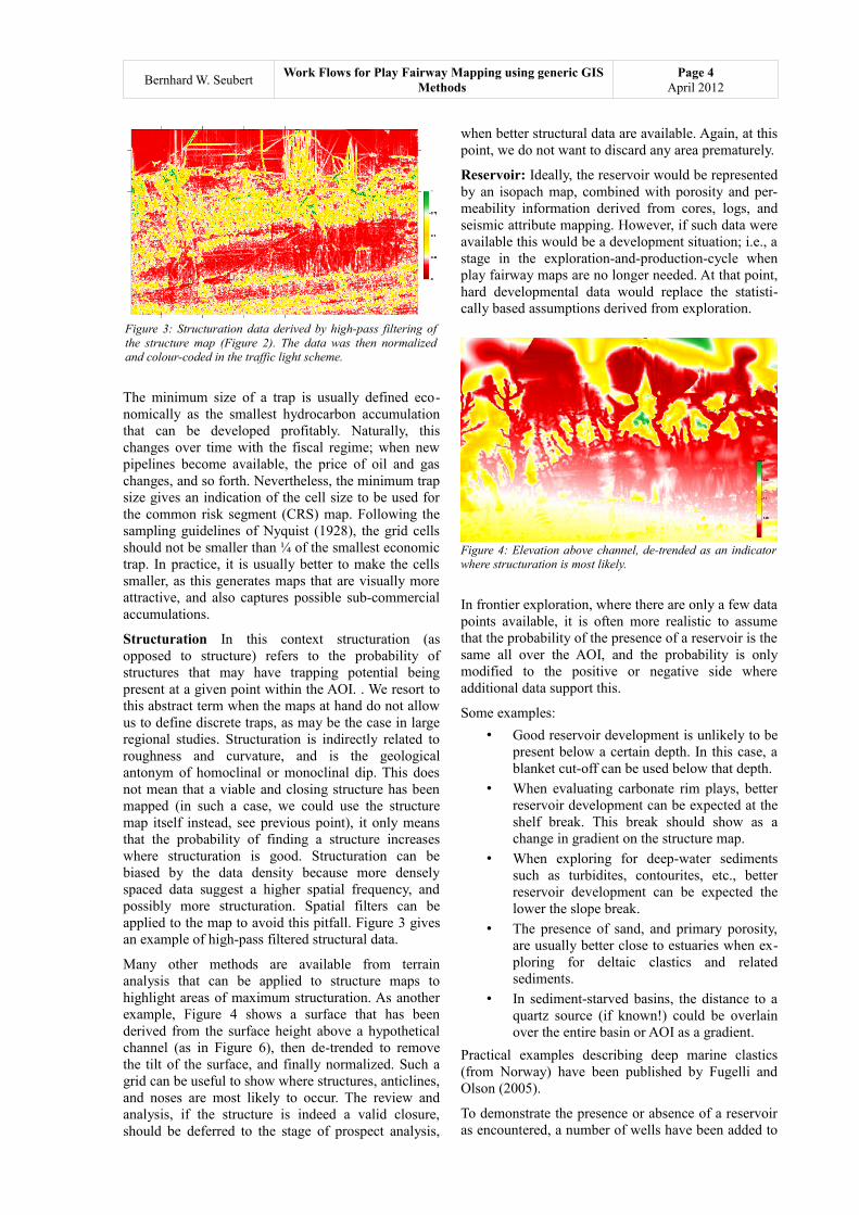
Structuration In this context structuration (as opposed to structure) refers to the probability of structures that may have trapping potential being present at a given point within the AOI. . We resort to this abstract term when the maps at hand do not allow us to define discrete traps, as may be the case in large regional studies. Structuration is indirectly related to roughness and curvature, and is the geological antonym of homoclinal or monoclinal dip. This does not mean that a viable and closing structure has been mapped (in such a case, we could use the structure map itself instead, see previous point), it only means that the probability of finding a structure increases where structuration is good. Structuration can be biased by the data density because more densely spaced data suggest a higher spatial frequency, and possibly more structuration. Spatial filters can be applied to the map to avoid this pitfall. Figure 3 gives an example of high-pass filtered structural data.

Many other methods are available from terrain analysis that can be applied to structure maps to highlight areas of maximum structuration. As another example, Figure 4 shows a surface that has been derived from the surface height above a hypothetical channel (as in Figure 6), then de-trended to remove the tilt of the surface, and finally normalized. Such a grid can be useful to show where structures, anticlines, and noses are most likely to occur. The review and analysis, if the structure is indeed a valid closure, should be deferred to the stage of prospect analysis,

when better structural data are available. Again, at this point, we do not want to discard any area prematurely.

Reservoir: Ideally, the reservoir would be represented by an isopach map, combined with porosity and per-meability information derived from cores, logs, and seismic attribute mapping. However, if such data were available this would be a development situation; i.e., a stage in the exploration-and-production-cycle when play fairway maps are no longer needed. At that point, hard developmental data would replace the statisti-cally based assumptions derived from exploration.

In frontier exploration, where there are only a few data points available, it is often more realistic to assume that the probability of the presence of a reservoir is the same all over the AOI, and the probability is only modified to the positive or negative side where additional data support this.

Some examples:

• Good reservoir development is unlikely to be present below a certain depth. In this case, a blanket cut-off can be used below that depth.

• When evaluating carbonate rim plays, better reservoir development can be expected at the shelf break. This break should show as a change in gradient on the structure map.

• When exploring for deep-water sediments such as turbidites, contourites, etc., better reservoir development can be expected the lower the slope break.

• The presence of sand, and primary porosity, are usually better close to estuaries when ex-ploring for deltaic clastics and related sediments.

• In sediment-starved basins, the distance to a quartz source (if known!) could be overlain over the entire basin or AOI as a gradient.

Practical examples describing deep marine clastics (from Norway) have been published by Fugelli and Olson (2005).

To demonstrate the presence or absence of a reservoir as encountered, a number of wells have been added to

Figure 4: Elevation above channel, de-trended as an indicator where structuration is most likely.

Figure 3: Structuration data derived by high-pass filtering of the structure map (Figure 2). The data was then normalized and colour-coded in the traffic light scheme.


Methods

April 2012

the basic structural data in Figure 2 and are shown in Figure 5.

Technically, the map representing the probability of reservoir presence can be compiled from several maps that depict and combine the various aspects of reservoir presence. For example, combining a sand/shale ratio map with a depth (~porosity) map may provide a more realistic view. When combining several maps into one petroleum systems element, a weighting could be introduced. Finally, the resulting composite map must be normalized (discussed later).

Even at this stage, it is clear how easily one may un-wittingly overcomplicate this process with the addition of extra algorithms, or other considerations. It is human nature to continue to add more detail if more information is available. However, it is crucial to consider how much another subtle modification would actually add to the final outcome, and whether the uncertainty in another element is so large that it outweighs such detailed treatment of one particular aspect.

Source and Maturity

This element is probably the most difficult to incorporate into PFM at an early stage. It also touches upon matters of coincidence (when, in geological time, did it reach maturity?) in conjunction with migration (e.g., if it was mature at time T, were the hydrocarbons expelled for migration at the same time or later, did they find a migration pathway, did the faults exist at the time of migration, and if so, did they impact upon the migration path?).

The sub-elements are:

Presence of Source: Owing to the notorious tendency of oil companies not to drill synclines, there are many mature and established petroleum provinces where the actual nature of the source (stratigraphic position, facies, activation energies, yield, etc.) is poorly con-strained by measurements, and often only inferred. At this point, we must be very careful not to assume that a lack of evidence for source presence means that that there is no source present.

Maturity and Timing: Did the source rock actually reach maturity? On a map, the area of probable maturity may be approximated by a depth map similar to Figure 8.

Other questions include: when was maturity reached? Was the source later overcooked, thus raising the risk of a fill and spill (gas replacement) situation?

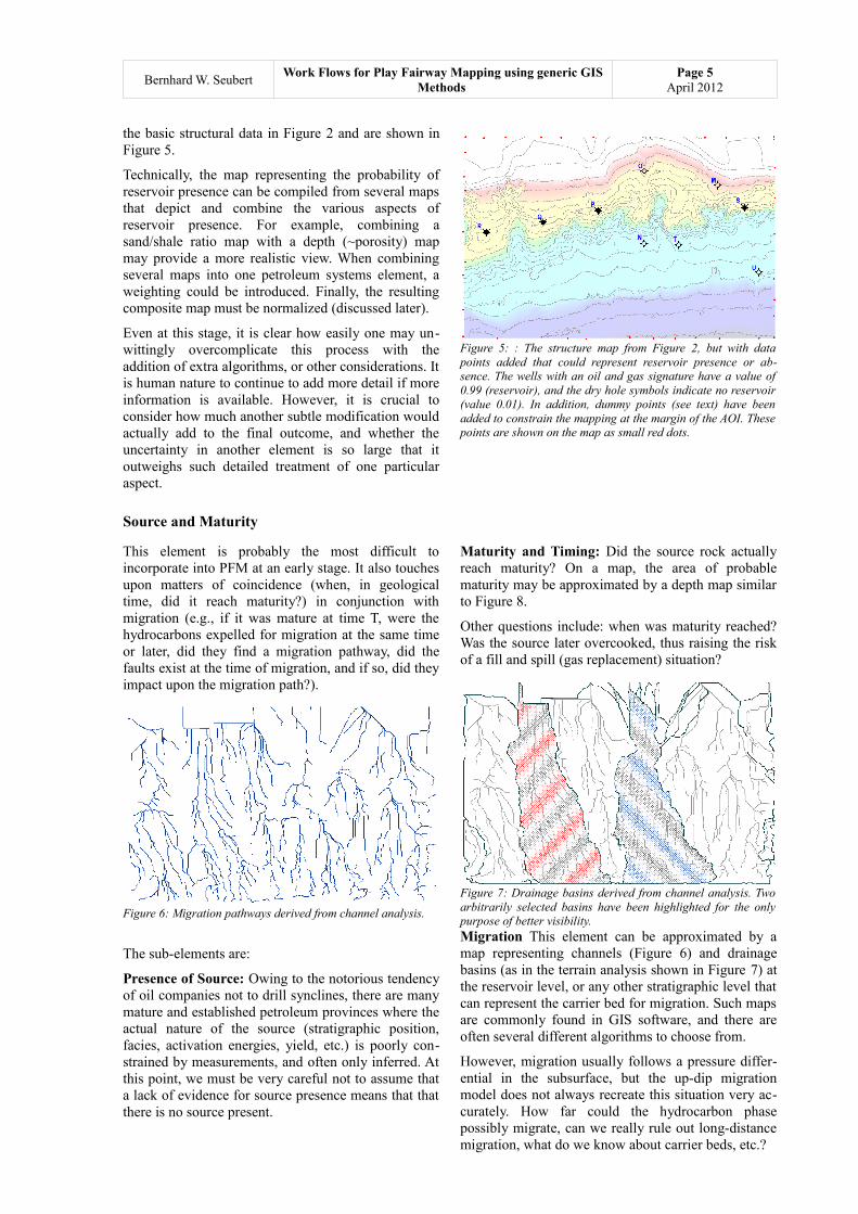
Migration This element can be approximated by a map representing channels (Figure 6) and drainage basins (as in the terrain analysis shown in Figure 7) at the reservoir level, or any other stratigraphic level that can represent the carrier bed for migration. Such maps are commonly found in GIS software, and there are often several different algorithms to choose from.

However, migration usually follows a pressure differ-ential in the subsurface, but the up-dip migration model does not always recreate this situation very ac-curately. How far could the hydrocarbon phase possibly migrate, can we really rule out long-distance migration, what do we know about carrier beds, etc.?

Figure 7: Drainage basins derived from channel analysis. Two arbitrarily selected basins have been highlighted for the only purpose of better visibility.

Figure 5: : The structure map from Figure 2, but with data points added that could represent reservoir presence or ab-sence. The wells with an oil and gas signature have a value of 0.99 (reservoir), and the dry hole symbols indicate no reservoir (value 0.01). In addition, dummy points (see text) have been added to constrain the mapping at the margin of the AOI. These points are shown on the map as small red dots.

Figure 6: Migration pathways derived from channel analysis.


Methods

April 2012

Another approach used to gauge the probability that a structure has received hydrocarbon charge is to add a buffer as an envelope around these channels. Such a buffer area would highlight those places where migrant hydrocarbons were more likely to reach a trap and fill it.

In Figure 15, the charge and migration model is much more basic than these illustrations might actually suggest. This simplification has been made to empha-size the flow, rather than details of the various possible map construction. In Figure 8, we assume that anything below –3900 m is in the oil window, and therefore has a 95% chance of being charged. Away

from the kitchen, it is simply assumed that the probability of charge decreases towards the northern margin of the map where it reaches the background value of 0.5 (50 percent).

As with the reservoir, when assessing matters of source presence, maturity, and migration, it is easy to become overly concerned with the many details of basin modeling, instead of concentrating on the main aim; i.e., to make a map that classifies the prospectiv-ity of an under-explored area into good, medium, and not good. Too much detail at this point may actually be counterproductive. Less is more!

Figure 8: For a basic evaluation, let us assume that the basin is filled with a source rock of constant thickness, which reaches maturity below a certain depth. The oil window is illustrated by a planar surface at –3900 m. The area up-dip of this kitchen could receive hydrocarbon charge that migrates out of this kitchen area. The area where charge is available to be trapped could be ap-proximated by a series of buffers (see Figure 11).


Methods

April 2012

Seal

Seal is the resistance of the overburden to hydraulic fracturing and/or seepage losses by means of over-coming the capillary entry pressure of the cap-rock.

In the first approximation, the seal capacity of a formation above a trap could be represented by its thickness (minus water depth). More useful, is a com-bination of thickness and bulk density (from logs or estimated from regional compaction curves).

If available, a map of the horizontal stress vectors would help to gauge the reduction in the maximum vertical stress before hydraulic fracturing occurs, and hence reduces the quality of the seal. Such maps

would be most useful in areas where thrust tectonic activity is known to occur or, even better, can be mapped by seismic survey or in outcrop.

In addition, any map that shows faults, or the density of fault traces per unit area, could be used to modify the basic overburden map to develop a better under-standing of the regional seal potential.

It is useful to note here that faults, if they can be mapped from the available data, can give an indication of the timing of structuration and matters of co-incidence (see next point).

Figure 9: Seal (the probability that hydrocarbon charge is retained in the trap) can, in the simplest cases, be represented by the overburden thickness. In this simplistic case, the normalized thickness between two surfaces is taken as a proxy for the seal capacity. For anything below –2000 m (the olive-green surface) seal is not relevant. Clearly, no seal is possible at zero depth (orange red sur -face). Anything in between is a linear interpolation, then normalized to 0 < z < 1.


Methods

April 2012

Coincidence The timing of events, or the critical moment; i.e., coincidence, is one of the more elusive elements. Fault patterns, and the fault density (fault traces per unit area), can provide some indication of whether the potential accumulation may have been destroyed over geological time. A more elegant re-presentation would be a surface defined by the envelope of fault traces in a section. The younger the fault envelope, the more unlikely that the trap has survived. Such mapping would require good dating of the sediment layers, something that is rarely available in rank exploration.

Timing, determining the ‘right moment’ or ‘critical moment’, is problematic, elusive, and usually evade proper treatment on a map. Unfortunately, this paper has little to add regarding a solution to this conundrum.

As may be appreciated already, there is a wide field of overlapping definitions and differences in usage employed by different companies and institutions. For example, seal, leakage, and trap integrity can be addressed from various angles. Some workers like to define a parameter named retention potential, which is a combination of seal and trap integrity (which has a component of timing), while others like to consider the trap only as the trapping structure, and deal with seal and integrity separately. All approaches are possible, and the generation of PFMs does not follow a single, unique path. After all, the purpose of PFMs is to arrive at a three-way classification of an area. As long as definitions and criteria are applied consistently across the AOI and map sheets, different approaches will, and do, lead to an appropriate answer.

Figure 10: The resulting seal probability map (based on the assumptions in Figure 9) might look like this. Note that the scale of this map is the probability that an effective seal does exist, not the actual value of the seal capacity, or the possible maximum column height

Good seal for theentire green area

Possible seal problemsin the yellow band

Red areas have asignificant seal risk


Methods

April 2012

Map Construction: Extrapolation Methods

In map analysis, Tobler’s first law of geography applies: ‘everything is related to everything else, but near things are more related than distant things’ (Tobler, 1970). At the other end of the spatial-scale spectrum, there is white map space, areas where abso-lutely nothing is known about a given property. This is related to the sill in kriging terminology (Figure 12). Therefore, an arbitrary background value must be assigned to the white map area. This value is based purely on assumptions about the unknown. A value of 0.5 (50% probability) is a good starting point, because it indicates that the element may, or may not, be present. In practical mapping, we may want to vary this 50% by ± 5% or less of spatial noise, spectral whitening if you will, to avoid contouring a flat surface, which often leads to ugly map artifacts, and without adding more information to the map.

In science, every measurement has an inherent element of uncertainty associated with it. Away from the control point where the measurement was taken, the uncertainty of the measurement in-creases. The method used to understand and describe how the un-certainty changes in all map directions varies, and is almost an art form. Krige (1951) proposed an elegant, but mathematically demanding, method that requires a good understanding of the statistical properties of the underlying popu-lation. More im-portantly, kriging re-quires a sufficient number of data points, which are often not available in frontier exploration. At this early stage, data are extrapolated from a very few data points by means of commonsense and speculation. In the early stages of exploration, primitive methods must replace kriging, which is best applied in a later stage such as during development, when more data is available and can get proper statistical treatment.

Nevertheless, at every step of the evaluation process we need to remind ourselves that when constructing PFMs we are assessing the probability of occurrence of something at a given point in map space, and at a location distal to our data points. So, how meaningful are the data points for something that is a significant distance away from them?

In the following section, a selection of the many available methods that can be used to fill map space with very few data points, and some good geological reasoning, will be discussed.

In this context, the art of mapping is one of relating the few data points available, and making assumptions regarding the properties of the white space. Without doubt, kriging is the most thorough and elegant method for this purpose. However, it is mathe-matically demanding, and therefore carries the risk that invalid relationships are buried deep in the mathe-matical formulae, which are difficult to untangle and opaque to management (who usually prefer a simple answer to a complex truth) Most importantly, kriging requires sufficient data.

In the following, this paper will discuss several of many methods and that can be employed to fill maps

space with very few data points and some good geological reasoning.

Extrapolation. To maintain simplicity, four fundamental algorithms of extrapolation are shown (Figure 14 a–e): linear, exponential, point-fitting (spline), and Voronoi polygons (shown in Figure 13). These are only a few of the possible algorithms that can be used to connect data points to the undefined white space, the average background. This shows that none of the conventional gridding and extrapolation methods is particularly useful when it comes to representing matters of reservoir presence, porosity, and formation thickness.

The buffer, is an envelope in a given distance from the data points. This “halo” relates to the distance between ‘nugget’ and ‘sill’ in Kriging (Figure 12).

Figure 11: Buffer rings with various values approaching the background value. The change in value occurs in constant distance from the control points (wells).

backgroundvalue, 0.5

more likely,~ 0.65

very likely,~ 0.09

less likely,~ 0.35

unlikely,~ 0.1


Methods

April 2012

Figure 11 also shows why considering such a buffer zone between the data point and the white map space may provide a better representation than extrapolation based on gridding. The corresponding profile through a buffer – or several buffer rings – would be a step function. One of the advantages of a buffer is that it can be further edited by hand to follow any guiding indicator. For example, instead of using a buffer ring with an arbitrary radius, the buffer could follow a mappable geological feature or seismic attribute. Again, with a view to more elaborate methods, this would be a simplified application of kriging with external drift.

Dummy values (point, linear, or area) may be added to the data set to further constrain mapping. The need to introduce such dummy values greatly depends on the gridding algorithm applied. Certain algorithms have the tendency to generate spurious results at the corners of the map, and in low data areas, because they tend to extrapolate the curvature or the change of curvature of the mapped surface. A few additional points added into the data list usually prevent this, and introduces more geological plausibility (see Figure 5).

Gradient, tilt, and trend surfaces are modifiers that may be applied in some situations to add a gradual bias to any given map. Trend surfaces can also be applied to cut through the mapped surface, for example to illustrate basinal areas, to highlight heights where erosion may have taken place, etc.

Such gradients, or gradient surfaces, can be con-structed with the usual GIS tools in two different ways.

• By defining and calculating the desired values at a given map location and compiling the data in a spreadsheet or in a CSV or other list format from which it can be gridded using the appropriate software and gridding algorithm.

• Alternatively, the desired feature can be digitized in a GIS program or helper application, and then the shape (point, line, or area) converted to a number of data points that can then be gridded.

Another approach, and an important manipulation, is to calculate a trend surface from the data. In the simplest case, a first-order trend surface is a tilted plane where exactly half of the grid cells are above the surface, and half below.

Figure 13: Voronoi polygons (i.e., Thiessen polygons) are constructed from separating lines that are exactly half-distance between two data points (the red arrow illustrates this). This extrapolation method is of limited value when constructing PFMs.

Figure 12: A variogram illustrating how the variance of a value to be mapped changes with distance away from the measure-ment point. At the measurement point itself, the variance can be zero or still have a non-zero value. The sill is the variance that is reached at ∞ distance. In practice, this sill variance is reached much earlier at a given range. Exactly how the variance changes away from the control point is a matter of fitting complex mathematical models to a data set.


Methods

April 2012

Figure 14: A synopsis (in 3D) of several methods used to extrapolate data into the map space. From top to bottom (a) using concentric buffer rings, (b) Voronoi polygons, a step function, (c) linear interpolation, and (d) a spline function that honors the data points, but gives a poor interpolation. Please refer to Figures 11 and 13 for an explanatory map view of the Voronoi and buffer functions.

(a)

(b)

(c)

(d)


Methods

April 2012

Map Construction: Normalization and corrective Multiplication Factors

Eventually, we will arrive—even though via different and play specific methods—at three, four, or even five maps that each represent the probability of petroleum system elements being present. Some companies use five elements, others four, or even only three elements. In the latter case, the company may address seal and coincidence under the aspect trap, with the consideration that a filled trap has structural integrity and seal, and was at the right place to receive charge.

The maps, each representing one petroleum systems element, are combined by grid multiplication, the dot product, or inner product of the matrices. To make this possible, the matrices must have the same dimensions of m and n. It is therefore important to define the map size, geographical coordinate system, grid, coverage, and number of nodes at the earliest possible stage of the project. Again, all maps that have been mentioned before must have the same size. Absent values (no data values) such as -999.25, 1 * 1031 or – even worse – zero, as they are implemented in certain software must be avoided at all cost. Consider the argument before: the maps show the probability of occurrence, it it is either there, not there or we don't know, – but absent values cannot exist.

However, before the maps of the various elements can be multiplied, care must be taken that the grid values of every map fall between 0 and 1. Again, there are several ways to achieve this, either:

• the map representing each petroleum system element already fulfills this requirement; i.e., all data are positive and fall between 0 and 1. This does not necessarily mean that the smallest value must be 0 and the largest 1 (c.f. prospect evaluation); or

• the grid must be normalized, or scaled, so that their values range from zero to one.

Note that both steps can lead to a different weighting of the petroleum systems elements. In my view, both may be correct depending upon the circumstances and purpose of the map.

Formula 2:Normalisation

For purposes of terminology, it is suggested that the terms ‘relative’ or ‘absolute’ are used when describing and discussing the results of the PFM constructed.

Furthermore, when multiplying maps with a different number of elements, the resulting middle value is different as shown here:

0.5∗0.5∗0.5 = 0.125 [three parameters ]0.5∗0.5∗0.5∗0.5 = 0.0625 [ four parameters]

0.5∗0.5∗0.5∗0.5∗0.5 = 0.0312 [ five parameters]

This relationship must be borne in mind when comparing PFMs made using a different number of elements, or when comparing PFMs to the outcome of prospect assessment and risking. Differences between the possible outcomes can be compensated for by using a corrective multiplication factor. For example, when comparing a four-parameter map with a five-parameter prospect evaluation, the latter should be multiplied by a factor of 0.5 to make the values com-parable. In calculus, this is the multiplication of a grid (or matrix) by a scalar. Multiplying by 0.5 does not in-troduce any bias, neither positive nor negative.

Drawing the various elements together, Figure 15 gives a visual representation of the matrix multi-plication of the various elements and the resulting map. The histogram (Figure 15h), provides an in-dication of a possible alternative interpretation of such a map. We see a clear modal maximum at about 0.125. This suggests that anything above this level could be regarded as more attractive for exploration.

Figure 15i, the summary of this exercise, is somewhat surprising, insofar as the (apparently) most promising areas coincide with those where there was no reservoir in the well data points. This strongly suggests that PFMs should only be used as a first-pass review tool to highlight the more interesting tracts of the AOI. A case-by-case investigation of the more interesting areas is always required.

Again, it is important to emphasize that every map, and every element, in Figure 15 could have been constructed in a number of different ways, and the choice of the most suitable method is based on the data available for a given area and the geological reality, or rather our perception of it.

anorm =a i − amin

amax − amin


Methods

April 2012

Figure 15: Summary of the work flow. The maps on the left are (color-coded) grids of the petroleum systems elements. The map on the right is the summary; i.e., the final PFM calculated by multiplication of the four grids. A histogram has been added as a key to understanding the distribution of the values. Finally, in the map at bottom right, the maximum levels of the PFM have been contoured, highlighted, and overlain onto the structure map from Figure 2.


Methods

April 2012

Discussion and Outlook

As with the transition from Newtonian physics to quantum physics, when attempting to model petro-leum systems based on insufficient data we have to rid ourselves of the notion that everything can be calcu-lated and predicted, if only we had enough data and the right algorithms. PFMs are used in the very early stages of exploration, precisely that time when there is very little known about the AOI, at a time when such data are not yet available and must be substituted with geological commonsense. We should not outsmart ourselves with elaborate algorithms that are unable to support the observations and data. More importantly, we need to remind ourselves that PFMs are nothing more than a three-way classification of an AOI that attempts to depict the probability of hydrocarbon occurrence at a given location. Even more importantly, we must ask ourselves ‘can we really rule out....?’, so that we do not run the risk of discarding prospective areas prematurely, a grave and costly mistake for an oil company to make.

As explorationists, we should not follow those naysayers (they are usually 80% right) who make a career out of being negative; even though the statistics are on their side. Drilling four or five dry wells before a discovery can be, and is, a profitable business, and many oil companies have repeatedly demonstrated this. Our purpose as explorers is to promote the, albeit unlikely, 20% chance of success and not to give up all too early.

Looking forward, other algorithms to map the proba-bility of hydrocarbon occurrence are possible. These are, for example, methods borrowed from population biology. The fundamental niche from biology would

then be the framework within which hydrocarbon ac-cumulations can exist (temperature, distance to source, just to name a few of the parameters). For example, source could be equated to food, nutrients in biology, and the total volume of food available. That may not be enough to sustain a population, or in hydrocarbon world, some traps may remain under-filled or not charged at all. A set of hydrocarbon accumulations that belong to one common play type could be seen as one species. The advantage of such a methodology is that it can address and evaluate several play types and their interdependency at the same time. For example, the primary accumulation (play A), and another play that depends on spill or leakage (play B) from A, could be modeled in a similar manner to prey and predator relationships in biology.

A further advantage of such an approach is that it can also illustrate the development of hydrocarbon distri-bution over geological time, instead of on a map showing a temporal snapshot at time zero. The approach of Tobler (1970) to modeling urban growth is an illustration of a similar concept. As irritating as such biological approaches may initially appear, we quickly appreciate that very similar laws govern both processes. Software for such simulations is widely available, and only our imagination limits the imple-mentation of such novel concepts in petroleum exploration. Moreover, the beauty of such time-lapse modeling is that we would look at, and evaluate, the intermediate stages of the development of the petroleum system. This allows for the review and plausibility-checking of intermediate stages, rather than considering only the map of the end product at geological time zero.

Summary

• PFMs constitute only a very basic three-way classification of an AOI. Care is required to avoid becoming overly focused on a single element when other elements remain rela-tively uncertain, as is often the case in the early stages of exploration.

• Care should also be taken not to discard part of the AOI too early in the cycle of evaluation. It is preferable, and economically more prudent, to err on the optimistic side.

• PFMs are compiled for one play-type only. Depending on the play-type, different ap-proaches and maps are necessary. Therefore, PFMs of different plays, or such maps origi-nating from different companies, cannot be directly compared.

• A correcting multiplier must be introduced when PFMs, or prospect evaluations based on three, four, or five elements, are related to each other.

Acknowledgments

Data: The grid data used for Figure in this paper are marine multi-beam bathymetry data from the Bremer Sub-basin in Australia. These data are available for download under Creative Common Attribution 3.0; the full citation for the data set can be found in Spinoccia (2011). The Bremer Sub-basin lies between Albany and Esperance in southern Western Australia. The

Bremer Sub-basin, referred to previously as the Albany Sub-basin of the Bremer Basin, extends over an area of 11500 km2 with water depths ranging from 100 to 4600 m.


Methods

April 2012

It is emphasize, that the grids, maps, and data shown in this context have no other purpose than the demon-stration of the concept.

This paper was prepared and solely funded by PT PetroPEP Nusantara, a company consulting in the field of petroleum geoscience, based and registered in Jakarta, Indonesia.

The opinions in this document are solely the profes-sional opinions and judgments of the author, and under no circumstances whatsoever reflect the thoughts, processes, or ideas of any company, institu-tion, or other legal entity.

Text References

Duff, B.A., and Hall, D.M., 1996, A model-based approach to evaluation of exploration opportunities, in Dore, A.G., and Sinding-Larsen, R., eds., Quantification and Prediction of Hydrocarbon Resources: Stavanger, Elsevier, Norwegian Petroleum Society Special Publications, p. 183-196.

Fugelli, E.M.G., and Olsen, T.R., 2005, Risk assessment and play fairway analysis in frontier basins: Part 2—Examples from offshore mid-Norway: Bulletin of the American Association of Petroleum Geologists, v. 89, no. 7, p. 883-896.

Grant, S., Milton, N., and Thompson, M., 1996, Play fairway analysis and risk mapping: an example using the Middle Jurassic Brent Group in the northern North Sea, in Dore, A.G., and Sinding-Larsen, R., eds., Quantification and Prediction of Hydrocarbon Resources: Stavanger, Elsevier, Norwegian Petroleum Society Special Publications, p. 167-181.

Krige, D.G., 1951, A statistical approach to some mine valuations and allied problems at the Witwatersrand, Master’s Thesis: Witwatersrand, South Africa, University of Witwatersrand.

Magoon, L.B., and Dow, W.G., 1994, The Petroleum System, Chapter 1, in The Petroleum System— from Source to Trap:

Tulsa, OK, The American Association of Petroleum Geologists (AAPG), Memoir 60, p. 3-24.

Nyquist, H., 1928, Certain Topics in Telegraph Transmission Theory: Transactions of the American Institute of Electrical Engineers, v. 47, p. 617-644.

Olaya, V., 2004, A gentle introduction to SAGA GIS: AESIADesarrollo y Proyectos Medioambientales, S.L., Madrid,Spain.

Sandwell, D. T., and Smith, W. H. F, 2009, Global marine gravity from retracked Geosat and ERS-1 altimetry: Ridge segmentation versus spreading rate: Journal of Geophysical Research, v. 114, no. B01411, 18p.

Spinoccia, M., 2011, XYZ multibeam bathymetric grids of the Bremer Sub-Basin: Canberra, Australia, Commonwealth Scientific and Industrial Research Organisation (CSIRO), 12 files 112Mb zipped.

Tobler, W.R.A., 1970, A computer movie simulating urban growth in the Detroit region: Economic Geography, v. 46, no. 2, p. 234-240.

Software References

Disclaimer: Note that neither the author nor the company PT PetroPEP Nusantara endorses or recommends any of these computer applications. Nor is it suggested that any or all of these programs are ‘fit for the purpose’.This is only an incomplete list that has been compiled for the sole purpose of providing a starting point for the reader when reviewing computer programs that may, or may not, be useful in the context of this document, or for a purpose related or consequential to the content of this document.

Boehner, J. et al., 2001, SAGA - System for Automated Geoscientific Analyses: Göttingen, Hamburg, - Germany. http://saga-gis.org.

Golden Software, Inc., 2011, Surfer, version 10,: Golden, CO. USA, Golden Software, Inc., Surface Mapping Systems. http://www.goldensoftware.com

MapWindow GIS Team, 2011, MapWindow Programmable Geographic Information System: Idaho Falls, USA, Idaho State University. http://www.mapwindow.org

Sherman, G.E (and his team), 2011, Quantum GIS (QGIS): Surface Mapping Systems. http://qgis.org/

This document titled “Work Flows for Play Fairway Mapping using generic GIS Methods” by Bernhard W. Seubert is licensed under a Creative Commons Attribution 3.0 Unported License.

The document was made available online as PDF document in May 2012 at http://www.petropep.com

http://saga-gis.org/

http://www.petropep.com/

http://creativecommons.org/licenses/by/3.0/



http://qgis.org/

http://www.mapwindow.org/

http://www.goldensoftware.com/

work flows for play fairway mapping using generic gis methods flows … · bernhard w. seubert work...

Documents