working paper series 2012 - eth z · international development issn 1470-2320 working paper series...

International Development

ISSN 1470-2320

Working paper Series 2012

No.12-128

The Demographic Dividend in India:

Gift or curse? A State level analysis on differing age structure and its implications for

India’s economic growth prospects

Vasundhra Thakur

Published: April 2012

Development Studies Institute

London School of Economics and Political Science

Houghton Street Tel: +44 (020) 7955 7425/6252

London Fax: +44 (020) 7955-6844

WC2A 2AE UK Email: [email protected]

Web site: www.lse.ac.uk/depts/ID

of 29

- Abstract The age structure of a population plays a key role in promoting economic growth through an increase in the ratio of the working age population. This positive influence is conditioned on the presence of good policies and institutions. India is experiencing an unprecedented increase in the working age ratio and this is being hailed as India’s opportunity to undergo faster growth. This paper shows that the age structure is not homogenous throughout the Indian States. Whether India will be able to capitalize on its favorable age structure depends on how well the BIMARU states are able to reform their economy.

of 29

CONTENTS

1. Introduction 4

2. Relationship between Demographic Change and Economic Growth 6

3. Theoretical Background 8 3.1 The Demographic Transition Theory 8 3.2 Theoretical Estimation: Age Structure and Economic Growth 11

4. Indian Demographic Trends 12

5. Empirical Estimation 14 5.1 Data Description and Summary Statistics 14 5.2 Empirical Evidence: Age Structure and Economic Growth 16

6. The Future of the Indian Demographic Dividend 18

7. Limitations and Extensions 23

8. Conclusion 23 Bibliography Appendix Appendix I: Stata Output Tables Tables Table 1: Summary Statistics over States and Time 15 Table 2: Growth Rate of Working Age Ratio of Select States 16 Table 3: Growth in Per Capita Income of Select States 16 Table 4: Working Age Ratio of Select States 16 Table 5: Regression Results 17 Table 6: Demographic Indicators India 2001:2025 19 Table 7: State Characteristics and Demographic Dividend in 2001 21 Table 8: State Characteristics and Demographic Dividend in 2026 21 Table 9: Percentage distribution of India’s Working Age Population by State 22 Figures Figure 1: Change in Working Age Ratio over time in select States 15

of 29

Section 1: Introduction The influence of population on macro-economic performance has long been debated upon by social scientists. Of the many aspects of population change, it is the size and growth rate of a population that has been at the fore of the debate. An emerging dimension of demography that has now entered the debate is the influence of age structure on economic growth. An increase in the share of the young working age group can be beneficial for growth because such people are more productive and contribute more to the economy. Due to the positive effects of an increase in the working age group, this bulk in the age structure is also called a ‘demographic dividend.’ However, there is nothing automatic about this dividend, if complementary institutions and policies are not in place, this dividend could turn out to be a ‘curse’ rather that a ‘gift’ because a large cohort of young unemployed people can turn into an economic disaster (explained in greater detail in next section). Given that the dimension of age structure has only recently got attention, comparatively few papers have been published which empirically analyze the phenomena. An influential paper by Bloom and Canning (2004) undertakes a cross-country analysis from 1965 to 1995. They find that a favorable age structure has a positive impact on income growth provided that the country has a high degree of openness to trade. Several papers have focused on a single country analysis. Estimates show that around one-third of the East Asian miracle can be attributed to experiencing a ‘demographic dividend’ (Bloom and Williamson, 1998; Bloom et al 2000; and Mason 2001). Similarly, Bloom et al (2007) carried out a similar exercise for Africa which still faces unfavorable demographic factors; they find that Africa is on the brink of earning the demographic dividend. However, they remain cautious about this translating into economic growth because to harness the dividend efficiently, good institutions must be in place. While some African countries have undergone institutional reform, the others countries facing significant increases in their productive age groups like Ghana, Malawi and Namibia need to improve their institutional and policy environment. India is the country of interest for this paper. The motivation for the studying India is compelling: it is both a demographic and an (emerging) economic giant in the world. It is home to around 17.5% of the world’s population and one in every six person in this world is an Indian. Additionally, India is a continuing force on the global economic scene. According to the World Bank, while India grew at 9.7% in 2010, the developed economies of the world had a dismal performance with the USA growing at only 2.9%, United Kingdom at 1.3% and Germany at 3.6%. At present, India is identified as undergoing the demographic transition. With a median age of 22.5 years and a dependency ratio of just a little above 0.4, a ‘demographic dividend’ in India is currently underway (Registrar General of India, 2001). Given the sheer size of India’s population, how it deals with the ‘demographic dividend’ has consequences for the entire world. At present, there is much excitement over the Indian demographic transition and its possible effects on growth. Lee (2003) estimates that even if income per person remains constant, a decrease in dependents will boost income per capita by 22%. Observers note that India’s long term growth prospects look particularly positive compared to China on the grounds that while the latter has already undergone the demographic transition by artificially inducing it through its one-child policy and is now rapidly aging, India is only on the cusp of receiving a demographic dividend (Nilekani, 2009; Economist 2011). Newspapers, both local and global, are rife with references to the dividend as a route for India to develop its economy while at the same time emphasizing that jobs, education and skills will have to be developed for a

of 29

positive effect (Basu, 2007; and Sabhrawal, 2011). While the optimism for India’s future due to the demographic dividend is understandably held back because the country as a whole has to undergo many reforms to fully reap the demographic dividend, a critical component is being missed out; inter-state variations. India is not undergoing a homogenous demographic transition and some States are deep into the transition while some have only just begun. The southern states of Kerala and Tamil Nadu have already received most of the demographic dividend and the growth in their working age ratio is declining whereas the BIMARU states (consisting of Bihar, Madhya Pradesh, Rajasthan and Uttar Pradesh) just starting and their working age ratio is rapidly increasing. These BIMARU states typically underperform compared to the rest of the Indian States and the acronym taken in its literal sense means ‘unwell’ in the Hindi language. The main aim of this paper is two-fold. The first is to examine the impact of age structure on economic growth across Indian States. The second aim is to analyze whether the positive relationship which has historically been experienced in India between working age ratios and economic growth is at serious risk of altering with the BIMARU states entering into the demographic transition. The issue of divergence between Indian States has been discussed in the literature. Bose (2007) finds that there is a growing North-South divide in India in terms in most demographic and health dimensions. There will continue to be a population explosion in the northern BIMARU states. Oddly, given the excitement around the Indian demographic dividend, only a handful of academic papers have been published which rigorously test for the size and potential of the Indian dividend. James (2008) tests for the relationship between growth of the working age population and growth rate of income per capita 1971-2001. Though the author confirms the positive effect of a large working age population on economic growth, his analysis does not test for the growth in the share of the working age population. Thus the hypothesis does not isolate the difference between overall population growth which takes place in all age groups including the working age ones and a demographic dividend where population growth occurs mostly in the working age groups. Kumar (2010) overcomes this deficiency by introducing a variable for growth in the share of working age populations. The author estimates the relationship over 1981-2001 and finds that in the past, Indian States with a higher ratio of working age populations grew faster than the rest. However, looking at the future the paper remains skeptical about growth prospects for India citing that the BIMARU States will contribute over 52% of the increase in the working age populations which have poor infrastructure and policies to absorb the growing workforce in their economies. However, Aiyar and Mody (2011) who also confirm similar results remains optimistic citing that the demographic dividend which will mostly take place in the northern lagging States will present them with a chance to converge and catch up with the southern and western States who will face a reduction in their share of working age population. This paper goes a step ahead of rest of the literature and estimates the relationship with updated data for the decade 2001-2011, which no paper to the best of my knowledge has done yet. Most of the literature has found that till 2001, there is a positive influence of growth in working age ratio on economic growth and could only guess for the future impact of the emergence of the BIMARU states in receiving the demographic dividend. However, as rapid growth in working age ratio is being experienced in the backward Indian States, contrary to previous literature, this paper finds that it has overall negative consequences for economic growth. This negative relation is driven by the fact that appropriate policies and institutions

of 29

are not in place in these backward states to capitalize on the demographic dividend. However, this trend is not irrevocable. These backward states have only just started experiencing rapid growth in their working age ratios and will not lead the country in terms of an actual working age ratio much after 2026. To overturn this negative trend, targeted policies and interventions (identified in the next section) need to be undertaken now on an urgent basis. The rest of the paper is organized as follows. Section 2 follows the evolution of the debate on the relationship between demographic change and economic growth. Section 3 will flesh out a theoretical framework for the rest of the paper. First the demographic transition theory will be discussed and the channels through which the demographic dividend influences growth. Section 3 will also derive a theoretical estimation for the relationship between age structure and economic growth. Next an empirical exercise will be carried out to test the derived theory in section 4. Section 5 will discuss the future of the Indian demographic dividend in light of population projections and lastly Section 6 and 7 will discuss the limitation of this study and conclude. SECTION 2: Relationship between Demographic Change and Economic Growth The general consensus on the relationship between demographic vectors and economic growth has changed a lot over years. The arguments have touched on opposite ends of the spectrum where some argue that sustained population growth will be catastrophic while some argue that it will lead to more affluence. Broadly speaking, there are three schools of thought to this debate, namely; optimistic, pessimistic and neutral. Pessimistic School The debate can be traced back to the 1790s where the pessimistic school held much sway. Thomas Malthus is seen as the founding father of the pessimist school which foresaw doom if population growth was left unchecked. Their ideas were grounded in the theory of diminishing returns to scale put forward by David Ricardo, the pessimistic approach earning the theory to be named as a ‘dismal science’ (Reinhart, 2007:75). Malthus had stressed that societies with high fertility rates would have lower income levels than those with lower rates because high population levels would drive down the price of labor and increase the price of food. He argued that increase in food production would not be able to keep up with increase in population because while population grew geometrically, food production only increased arithmetically (Malthus, 1798). He believed that nature had its own checks to balance the world’s population. An increase in population would depress wages and lead to a shortage of food. As a result, there would be widespread starvation and famines and the population would come back to equilibrium. The other pessimistic view about high population growth is that of resource dilution. A growing population leads to a dilution of capital since it now needs to be shared amongst more people. Most of the pessimism was directed at the developing economies of the world where high population growth and low income levels existed and the pessimists believed this to be no coincidence. Optimistic school The pessimism gave way to a more optimistic view on population growth. While there was a massive growth in population the predicted disasters never materialized. World population had exploded in just 50 years from 2.5 billion in 1950 to 6 billion in 2000, instead of declining per capita income actually has instead grown exponentially (Birdsall et al, 2001). The optimistic school is grounded in the realization of economies of scale and specialization. Connections were made between population growth, innovation and increasing returns to scale. The line of argument goes that as the stock of human population grows so does the

of 29

stock of human capital; which is a major contributor to economic growth (Kuznets, 1967; Simon, 1981). Optimists have stressed that increased population would pressurize humans to innovate and find new ways of sustaining themselves. Following this reasoning, Simon concluded that in the long run, the prices of natural resources tended to decline rather than the other way round. While increasing returns to scale have usually been viewed as the being limited to the manufacturing and services sector, a surge in productivity have also been witnessed in the agriculture sector with the ‘green revolution.’ Esther Boserup, who specializes in the field of food production shows how similar pressure induced innovation in the field of food production. Rising populations have induced humans to innovate and food production technologies have constantly evolved since the beginning of time (Boserup 1965). The recent green revolution which uses intensive farming, irrigation, fertilizer and hybrid seeds has improved agriculture production markedly around the world. The Revisionists Following soon at the heels of the optimists is the more neutralist point of view. Here population growth is thought to neither hinder nor promote economic growth. Countries with weak institutions typically also had high population growth and the effect of these two aspects needed to be isolated. So while rapid population growth had an overall negative effect on the economy, this causation was weakened when one took into account the country specific characteristics of institutions, policies, markets and technology (Birdsall et al, 2001). Bloom and Canning (2004) contend that this consensus led to population and reproductive health as a potential determinant of economic growth being given a backseat by key development agencies. Age Structure Recently a new dimension of demography is being discussed which challenges the revisionist view and places changes in population characteristics as a major determinant of economic growth; age structure. Namely that an increase in the share of the working age group; identified in this paper as between 15-59 years of age, will have a positive impact on economic growth. This theory is influenced by the Life Cycle Hypothesis and the human capital approach (Navaneetham 2002). The Life Cycle Hypothesis fleshed out by Franco Modigliani in the 1950s posits that the level of income varies systematically over the different phases of a person’s life cycle. In order to achieve a smooth consumption throughout the period of their lives, a person’s level of savings fluctuates over different cycles (Modigliani 1988). Thus, a person’s behavior alters as he/she passes through different age groups, which translates into different economic outcomes over time. A young child is simply a net consumer and investments are needed for the child’s health, education and other needs. However, a person becomes a net producer when he/she moves into the working age group. The person supports his/her dependents and at the same time will save for their retirement when their productivity levels are not expected to be as high. As old age dawns, the person is again a net consumer living off what they had saved in the past. This micro-level behavior has big implications for the economy as a whole. A country with a favorable age structure, i.e. a decline in the dependency ratio people will be able to save more rather than diverting their excess incomes towards the upkeep of their dependents. It is a common economic assumption that savings equal investment (Keynes, 1936). If all the savings are diverted towards productive investments, faster economic growth will be experienced.

of 29

Interestingly the pessimistic school of thought was well aware of the consequences of age structure. However, given that the age structure when they were researching the low income countries was characterized as having a large number of young dependents, they only drew out negative conclusions from their analysis. Coale and Hoover (1958) on studying India and Mexico’s rapid population growth found high fertility and mortality rates. As a result, the countries had high dependency ratio with an extremely young population. They concluded that having a high ratio of dependents who lesser chances of surviving led to resource dilution and non-productive consumption diverted finds away productive investment. However, age structures do not remain constant and they do change as a country embarks on the demographic transition (explained below in the next section). As the age structure becomes more favorable in the working age populations, conditions become more conducive for economic growth. Depending on the policy environment, this increase in labor supply can generate more output in the economy. Also with fewer dependents, the economy will be able to save more which translates into greater investment rates. The implications of a change in age structure on economic growth can be immense. Bloom and Williamson (1998) attribute almost a third of the East Asian miracle to a favorable age structure i.e. an increase in labor supply. The next section will explain in detail the demographic transition which causes a change in the age structure of a population. It will also elaborate on how it influences economic growth and the complementary tools which are needed to capitalize on the favorable age structure. Section 3. Theoretical Background Section 3.1. The Demographic Transition Theory The demographic transition can be defined as a process where “societies experience modernization and progress from a pre-modern regime of high fertility and high mortality to a postmodern one in which both are low (Kirk, 1996:361). The transition is a worldwide phenomenon and is experienced by every country as it embarks on economic and social development. Since modernization has taken place at different time periods in different regions, the demographic transition has also occurred at different times across the world. The transitions first took place in North Western Europe with a decline in mortality around the 1800s. Eastern and Southern Europe soon followed suit. However, lower income countries did not start their transitions until the early twentieth century and took off especially after the World War II (Lee 2003). A striking fact about the current transitions is the speed by which they are being played out. According to Kirk (1996), the mortality transition took about 75-100 years in Northern Europe. This decreased to only 20-25 years in Eastern Europe. The current transitions taking place in developing countries are undergoing change even faster. Another interesting trend is that mortality decline is taking place even in conditions of low income. This is probably because of the spillover effects of advances in medicinal technology and scientific breakthroughs for curing many diseases. The demographic transition can be classified into 3 stages. In the first phase, both fertility and mortality rates are high. Here, the economy is in a Malthusian trap where any population growth will be kept in control through ‘preventive’ and ‘positive’ checks. The second phase kicks off with a fall in mortality. The mortality decline in the eighteenth century can be attributed to development of the modern state, establishment of law and order which oversaw reduction of deaths from random and local wars (Kirk, 1996). Human longevity is

of 29

also a consequence of medical breakthroughs in medicine, improvements in transport and agriculture, which help avert famines and improves nutrition. In almost all the countries where the demographic transition took place earlier, it took place in the conditions of rising incomes. A major difference being experienced in the contemporary transitioning countries is that mortality rates are falling without much increase in income, i.e. income growth is a sufficient but not necessary prerequisite for starting the demographic transition. Once mortality decline is underway, fertility decline follows next. The causes of fertility decline are much debated upon. Perhaps the most important determinant is the preceding decline in mortality. The basic economic theory of fertility states that every couple wishes to have an ideal number of surviving children. In conditions of high mortality they produce more children. However, in the face of declining mortality, they witness an increase in the number of surviving children and adjust their fertility rates accordingly (Lee, 2003). The impact of contraceptive technology and family planning is contentious. The author of this paper believes that contraceptive technology is simply a tool rather than a cause for declining fertility. Faced with changing preferences and lower mortality, people decline their fertility through all means possible. During the spectacular fertility decline experienced in Japan in the 1950s, a survey showed that around a third of all couples had practiced contraception at some point and sterilization was also widely used (Davis, 1963). While Japan had high tolerance levels of such tools, in places where contraception was looked down upon people responded through other means like late marriage, increased celibacy etc. Of course, there are more dimensions to this debate. Fertility decline is caused by a set of complicated and inter woven factors. However, it will go beyond the scope of this paper to address all the different strands of literature discussing causes of fertility decline. Fertility decline occurs after mortality decline almost always with a lag of a generation or two. Due to this lag there is a period where the same number of children are being born, however their chances of surviving has increased. Thus the second phase is characterized by rapid population growth and resulting changes in age structure and dependency ratios. The third phase starts when both fertility and mortality rates are low and the population growth stabilizes (Lee, 2003). In the first stage, the median population age is very young and population growth very low. In the second stage, when mortality falls, there is a population explosion and child dependency ratios rise rapidly. Once fertility levels also fall, the population growth is kept in check. However, this lag has many implications on age structure where there is a generation or two of rapid population growth which gives rise to the term ‘baby boomers’. As these baby boomers transition through different age groups, the age structure of the total population is skewed towards that particular age group. It is when this bulk of population enters the working age group; it is referred to as the demographic dividend. In this case, majority of the population is concentrated in the 15-59 age group and total dependency ratios fall to unprecedented levels. However, in the third phase, as a result of increased life expectancy, the median age goes up and old age dependency ratio grows. At the end of the transition, the total dependency is back to the initial levels, however there are now more elderly than children (Lee, 2003) Potential Benefits of the Demographic Dividend The benefits of having an age structure with more working age people and lesser dependents works through many mechanisms;

of 29

The most obvious benefit comes from having a bigger labor force. A larger share of people who are productive and able to contribute positively to the economy can be beneficial for economic growth (Bloom et al, 2003). Another aspect of the demographic transition is that of greater female emancipation. Lower fertility rates and longer lives create conditions for greater female empowerment as they find more time to break away from their traditional roles within the household and seek to join the labor force (McNay, 2005; Sen, 2000). An interesting example is from the experience of Indonesia where a fall in fertility rates was recorded from 5.5 births per woman to only 2.6 births from 1950 to 1999. At the same time, female labor participation rates increased from 30.6% to 53.2% (Bauer, 2001). This influx of female labor also adds to the above mentioned channel of increased labor supply. According to estimates, greater female agency played an important part in the East Asian miracle by women joining the labor force and keeping wages low while the countries pursued export led industrialization (Ibid). Furthermore, empowered women are more likely to educate, spend resources on their child health, which contributes to building human capital (Dreze et al, 1996). An important channel through which the benefit of the dividend manifests is an increase in the savings rate. Following from the Life Cycle Hypothesis, a person saves more when they are in their productive years for their retirement. In the conditions of a demographic dividend, an economy will save even more because there are fewer number of dependents and hence the resources which would have been consumed by the dependents can instead be saved. Several papers have found a positive relationship between a greater working age ratio and national savings rate (Kelley and Schmidt, 1996; and Mason, 1987) Private household savings play an important part in economic growth as seen in East Asia where it provided capital accumulation which fueled growth (Krugman 1994). The transition also brings about a change in human behavior. While it is difficult to fully measure this impact, having longer lives, lesser children and a better quality of life changes people’s attitudes and values in life. People begin to value education and health more, spend more on lesser number of children and can make long term plans, which they couldn’t do earlier (Bloom et al, 2002). Capitalizing on the Demographic Dividend It must be stressed that there is nothing automatic about translating the demographic dividend into a gift. All the above mentioned mechanisms just provide an opportunity for growth and achieving that depends heavily on the policy and institutional environment. Bloom et al (2002) identify a few variables namely; health, family planning, education and economic policies which must be prioritized to make good use of a demographic dividend. New economic activities will be generated due to an increase in the share of workers. However, care must be taken to ensure that the right kind of economic activities are generated. Economic activities can be divided into two types; Schumpeterian and Malthusian activities (Reinhart, 2007). Schumpeterian activities have the characteristics of increasing returns to scale, employing skilled and healthy labor and economic environment with imperfect competition, stable prices and sticky wages all of which creates a burgeoning middle class. Malthusian activities on the other hand have diminishing returns, unskilled labor and an inhibitory economic environment and whatever gains are made accrue to a select elite few (Ibid). Merging the policies identified in Bloom et al (2003) with the

of 29

distinction between good and bad economic activities this paper identifies the priority areas which need to be addressed to maximize the demographic gift. i) The biggest challenge and a critical factor to harnessing the demographic dividend is providing productive employment for the growth in the worker supply. Having a growth in the workforce is of no use until they have jobs through which they can contribute to the economy. However, a distinction must be made between simple low paid jobs which do not contribute anything beyond simple sustenance and productive jobs which enhance innovation and accelerate economic growth. On the contrary if job creation is not enough to absorb the bulge in labour supply, the country will be in a position with a large cohort of young unemployed people who have no future prospects and will be prone to violence and crime (Cincotta et al, 2003). ii) While the demographic transition plays out on its own, health and family planning policies can magnify the demographic trends taking place. The transition only starts with improvements in the public health. This includes lowering the infant mortality rate, improving maternal health and general health and sanitation improvements to ensure that that the quality and length of life is extended. A resulting drop in mortality will put into motion the mechanisms of the demographic transition which is necessary to cause a change in the age structures. Reducing fertility is an important aspect of the transition. Therefore it is imperative that family planning is encouraged. As mortality decreases, the ideal family size for households also decreases. Knowledge about the various tools of family planning and couples need for contraception must be met so that they can make optimum decisions about reducing fertility in the face of declining mortality. iii) Building human capital is essential and having a young population is not enough until they have certain skills to contribute effectively to the economy. In addition to starting the transition, health improvements are also needed to ensure a healthy workforce which can undertake Schumpeterian activities. Education is very important to build up the human capital so that a skilled workforce is present which can innovate and promote faster growth. Thus what policies are undertaken by a country experiencing an increasing share of workers will decide whether the chance is seized to create rapid economic growth or the country slips into a Malthusian trap. Section 3.2. Theoretical Estimation: Age Structure and Economic Growth In order to examine the impact of age structure we derive a theoretical model of estimation borrowed from Barro and Sala-i-Martin (2004) and used by various papers studying a similar relationship. (Bloom and Canning, 2004; Aiyar and Mody, 2011). Following Barro and Sala-i-Martin’s extensively researched model of economic growth, every country converges to its steady State from its initial State. g(z) = λ (z*-z0) Here z represents the income per worker. z* is the steady State of income per worker and z0 is the initial income per worker. λ is the speed with which a country converges to its steady State level. Now, the steady State income per worker is determined by many variables which impact worker productivity. Taking this into account, the above model can be re-written as;

of 29

g(z) = λ(Xβ - z0) (1) Where X represents all the variables that impact human productivity and β is its beta coefficients. To theorize the relationship between the variables of interest; share of working age population and income per capita, one follows the estimation derived in Bloom and Canning (2004). A simple relationship can be written as

(2)

Here, N is the total population, WA is the working age population, L represents the labor force and Y is the total income. Thus, the above equation simply states that income per capita is equal to income per worker multiplied by the labor absorption rate in the economy and the share of working age population. Substituting, Log (Y/N) = y; Log(Y/L) = z; Log (L/WA) = p; Log (WA/N) = w We can rewrite (2) as; y = z + p + w (3) For simplicity one will assume that the absorption rate is constant. Deriving this equation in terms of growth, g(y) = g(z) + g(w) (4) Now, substituting (1) and (2) into (3), we get g(y) = λ (Xβ - z0) + g(w) g(y) = λ (Xβ +p+ w0-y0)+ g(w) (5) Equation (5) will form the base of the empirical strategy. Here growth of income per capita is dependent on the initial share of working age population, initial income per capita, growth rate of working age population, participation rate and other variables affecting human productivity. This paper is not interested in the participation rate and one will assume that it will be captured in the constant term the empirical exercise is carried out. Section IV: India Demographic Variables and Trends Aggregate demographic changes have been impressive in India. Mortality indicators have fallen dramatically and estimates show that life expectancy grew from 24 years in 1920 to 62 years recently. This is an increase of 0.48 years per calendar year (Lee 2006:171). A fall in fertility rates has been more gradual but it has decreased nonetheless. In 1972, fertility rate was very high at 5.2 births per woman (SRS, Registrar General 2011). This estimate fell to 2.6 births in 2009. Similarly, dependency ratios have also fallen in India to around 0.4. However, taking country aggregate figures at its face value would not give an accurate picture of the different changes taking place within India. India is made up of 32 States and union

of 29

territories. There are huge differences on an inter-state level and economic, social and demographic indicators are far from homogenous. The 2008 fertility rate in India of 2.6 births masks large variations where below replacement level fertility rates have been achieved in Tamil Nadu while there are some States like Bihar where fertility rate is still high at 3.9 births. A recent survey by The Economist highlights the huge differences between different Indian States. The survey matched different Indian States to other countries of the world with similar levels of economic and demographic indicators. On a GDP per capita basis, the high performing State of Haryana has the same levels as that of the middle income country, Armenia and the worst performing State, Bihar’s income per capita is equivalent to one of the poorest countries in Africa, Eritrea. On the account of population, India’s most populous State, Uttar Pradesh fit in a population of 195.8 million in 2008 which was equal to the entire population of Brazil. Andhra Pradesh with a smaller population size was only comparable to Swaziland. These wide variations between States have had an impact on the characteristics of the Indian demographic transition. Overall, the demographic window of opportunity opened in the 1980s and is expected to play out till 2025 (Navaneetham, 2002 p.24). However, the transition is not taking place evenly within the country. In fact, the Indian demographic transition has been described to graphically look like a camels two humped back (Nilekani, 2009). Thus the States can be divided into two kinds, the demographic ‘leaders’ and the ‘laggards’. The demographically advanced States include Kerala, Tamil Nadu and Karnataka. These States have been estimated to have been receiving the demographic dividend until now and their window of opportunity is now gradually closing whereas, the window of opportunity has only recently opened for the laggards in 2001 and will continue to do so until 2031 (Navaneetham 2009, p.21). Net State Domestic Product per capita, an indicator for per capita income has also continued to diverge amongst States. In 1997-98, nine rich States of India1 contributed 58% to the national income whereas the backward States consisting of the four BIMARU States, Orissa and Assam contributed only 27% to the national income. This share has been falling over the years and in 2004, the backward States only contributed only 25% to the national income. While their share in national income had been decreasing, the share of the laggard States in total population has been increasing steadily (Khomiakova, 2008). The dissimilarities also extend themselves to the structural makeup of the State economies. The geographic distribution of manufacturing industry, services and agriculture is highly uneven. To give an overview of the structural make up of India, the Western region (Maharashtra, Gujarat) is made up of large industries and is well to do, the North Western States (Himachal Pradesh, Punjab and Haryana) are dominated by agriculture and prosperous as well. The Eastern States are moderately successful with agriculture and the Southern States (Karnataka, Andhra Pradesh, and Tamil Nadu) have a prosperous high-tech industry and service sector. The ill performing BIMARU States do not perform well in any of the three sectors (Ibid). Given these sizable inter-state variations, it is important than any discourse on the Indian demographic transition concentrates on the State level. As we can see, all Indian States are not receiving the demographic dividend at the same time. Therefore, to study the likelihood of

1 These rich States are Punjab, Maharashtra, Haryana, Gujarat, West Bengal, Karnataka, Kerala, Tamil Nadu and Andhra Pradesh.

of 29

India optimally harnessing the demographic dividend, one needs to identify where the greater incidence of an increase in the share of the working age populations is taking place and whether the policies in those States are conducive for reaping the dividend. Those cautious of the likely benefits of the demographic dividend in India point out that the largest population growth is taking place in the BIMARU States which have the lowest income per capita and contributes the least in all the three sectors of agriculture, industry and services. These States follow what Erik Reinhart would call a Malthusian model of growth. However, as is the critical argument of this paper, it is not the population growth but the age structure that matters when one is talking about the demographic ‘window of opportunity.’ There is of course no doubt that the BIMARU states are weighing down on the rest of the country both because of its demographic size and its poor economic performance. Nonetheless, when talking in the context of the demographic dividend, we must retain the focus on age structure rather that total population. Hence, whether the BIMARU States will hamper India’s chances of harnessing the demographic dividend depends on whether it is experiencing such a window of opportunity and is forgoing any chance of using it effectively. This paper will now first check whether the theoretical model of demographic change and economic growth holds true in practice and identify which States are currently experiencing a (and will continue to do so in the near future) demographic dividend and its implications for India’s economic future. Section 5: Empirical Estimation Section 5.1. Data Description and Summary Statistics A balanced panel dataset for 17 major Indian States with data with ten year intervals from 1981-2011 is being used. For the purpose of analysis, a database of income per capita, total population, age structure and other socio-economic indicators has been created for major Indian States by decade. Due to data constraints, only data from 20 out of 28 States could be used. Data on 7 union territories was also incomplete and because of their small size, they were dropped from the dataset. The remaining States accounted for 88% of the total population in India in 2001, thus they make a good representative sample. Adjustments were made to the data to account for the newly carved States of Jharkhand, Chattishgarh and Uttarkhand in 2000. For the sake of continuity, data for these States from 2001 were added to their parent States of Bihar, Madhya Pradesh and Uttar Pradesh to enable comparisons over the same geographical area consistently through time. The data on total population, age structure and literacy rate is from the successive decadal Census of India. Data on the age structure variable for the year 2011 are projected figures also released by the Census of India. Due to the reporting style of the Census, the working age population is defined as from 15-59 years and could not be extended to 64, as is conventional. Per capita income is calculated from data on the Net State Domestic Product (NSDP) released by the Central Statistics Organization and compiled by the EPW Research Foundation. Comparable data on NSDP were only available for the time period 1981, 1991, 2001 and 2011, which are indexed to the 1999-2000 constant prices. NSDP data prior to 1981 are indexed to 1970-1971 prices and could not be used for comparison. The National Human

of 29

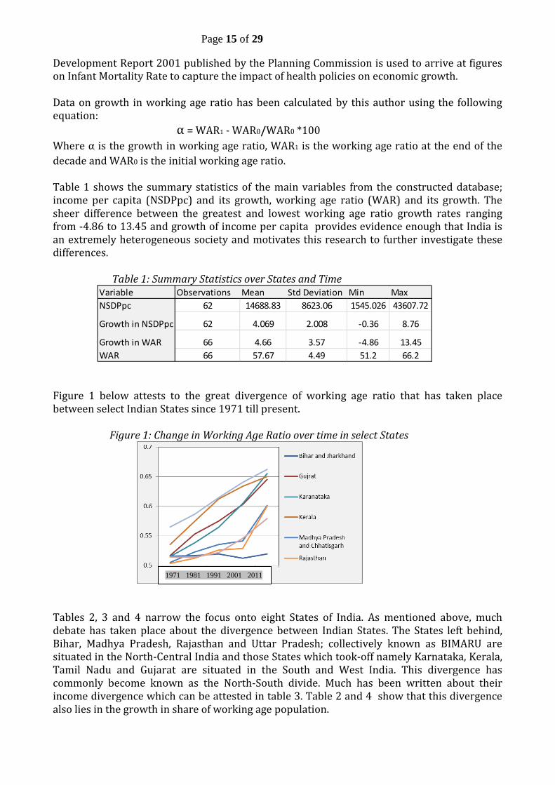
Development Report 2001 published by the Planning Commission is used to arrive at figures on Infant Mortality Rate to capture the impact of health policies on economic growth. Data on growth in working age ratio has been calculated by this author using the following equation: α = WAR1 - WAR0/WAR0 *100 Where α is the growth in working age ratio, WAR1 is the working age ratio at the end of the decade and WAR0 is the initial working age ratio. Table 1 shows the summary statistics of the main variables from the constructed database; income per capita (NSDPpc) and its growth, working age ratio (WAR) and its growth. The sheer difference between the greatest and lowest working age ratio growth rates ranging from -4.86 to 13.45 and growth of income per capita provides evidence enough that India is an extremely heterogeneous society and motivates this research to further investigate these differences. Table 1: Summary Statistics over States and Time

Variable Observations Mean Std Deviation Min MaxNSDPpc 62 14688.83 8623.06 1545.026 43607.72

Growth in NSDPpc 62 4.069 2.008 -0.36 8.76

Growth in WAR 66 4.66 3.57 -4.86 13.45WAR 66 57.67 4.49 51.2 66.2

Figure 1 below attests to the great divergence of working age ratio that has taken place between select Indian States since 1971 till present. Figure 1: Change in Working Age Ratio over time in select States

Tables 2, 3 and 4 narrow the focus onto eight States of India. As mentioned above, much debate has taken place about the divergence between Indian States. The States left behind, Bihar, Madhya Pradesh, Rajasthan and Uttar Pradesh; collectively known as BIMARU are situated in the North-Central India and those States which took-off namely Karnataka, Kerala, Tamil Nadu and Gujarat are situated in the South and West India. This divergence has commonly become known as the North-South divide. Much has been written about their income divergence which can be attested in table 3. Table 2 and 4 show that this divergence also lies in the growth in share of working age population.

1971 1981 1991 2001 2011

of 29

Table 2 and 3

Table 4

In 1971, the differences between the laggard and leading States were not that pronounced. However, by 2011 these differences have been magnified by a big factor. As an example, in 1971 the share of working age population was 51.5% and 56.5% in laggard Bihar and leader Tamil Nadu respectively. However, by 2011 the gap has increased to 52% in Bihar and 66% in Tamil Nadu. Similar trends can be found in growth of income per capita as well. These statistics can intuitively dictate that the changes in economic growth are anchored in demographic dynamics. The next section will test for this relationship by conducting an empirical estimation. Section 4.2. Empirical Evidence: Age Structure and Economic Growth Using the constructed dataset for 17 major Indian States for the period 1981-2011, one will gauge the impact of the share of working age ratio on economic growth. From the derived theoretical framework in Section 3.2, the paper will estimate various specifications of the following equation (5) as following: g_NSDPpci,t = β1NSDPpc,i,t-1 + β2WARi,t-1 + β3g_WARi,t-1 + γ’Xit +fi +ηt+ εi,t (6)

of 29

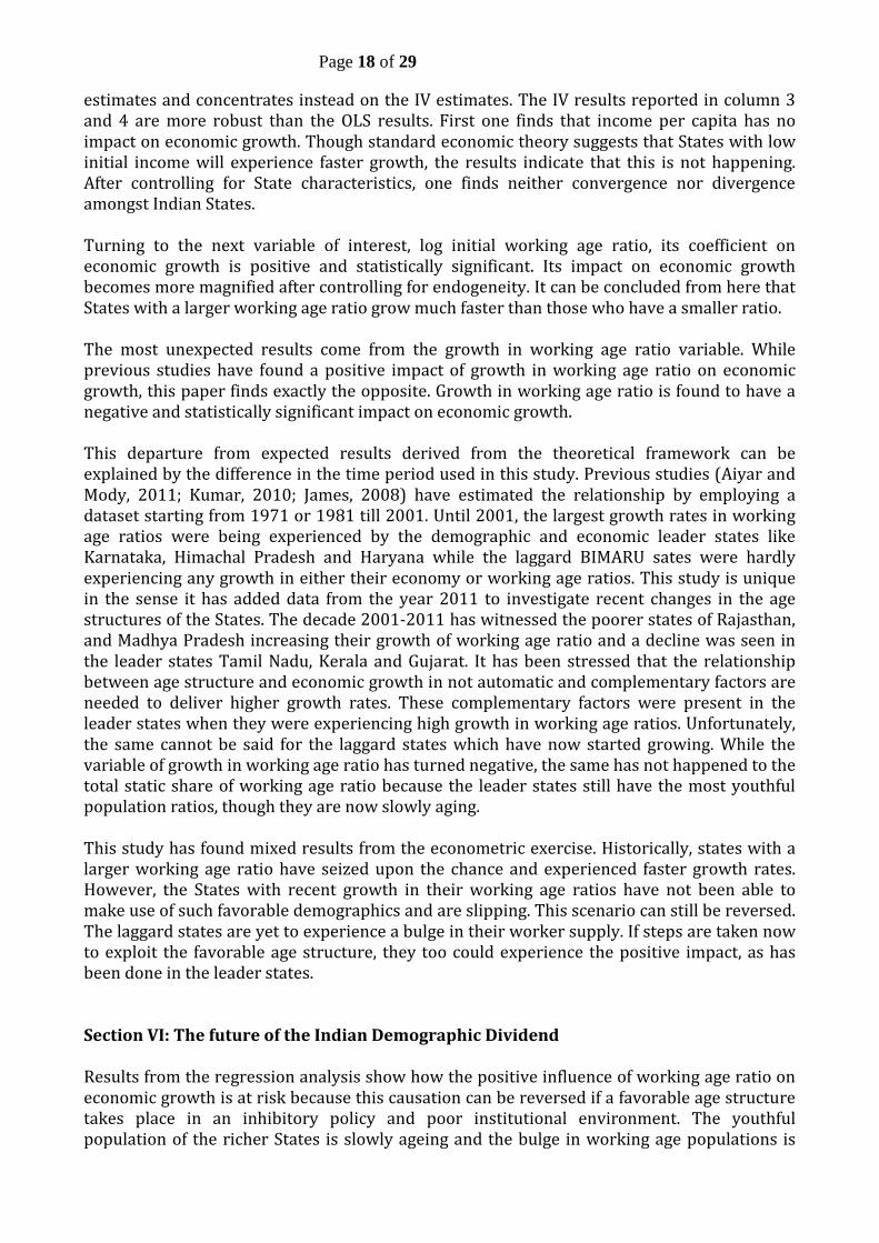
Where the g_NSDPpci,t is the annual average per capita NSDP growth (growth in income per capita) over the previous 10 year period. NSDPpc,i,t-1 is the initial income per capita at the beginning of the 10 year period, WARi,t-1 is the initial working age ratio in the total population at the beginning of the 10 year period and g_WARi,t-1 is the growth in the share of working age ratio over the 10 year period. X represents the control variables we have included in the estimations which might impact steady state labor productivity. Literacy rate has been used as an indicator of quality of labor and infant mortality rate (number if infant deaths per 1000 births) is used as a proxy for health status in the economy and total fertility rate is used as a proxy for women’s agency and the current state of the demographic transition. Time and State specific fixed effects are included to control any time or state specific shocks. Table 5 presents the results from the estimation. The first and second column presents the results from the simple OLS regression. A random effects model has been used which was chosen after running a Hausman test which indicated that the error term was not correlated with the regressors. Here the signs of the variables are as expected, however only the log of initial working age ratio appears to be significant. A greater initial working age ratio appears to have a large, positive and statistically significant impact on growth rate. In column 2 the control variable are added and none appear to be statistically significant. Table 5: Regression Results

Such poor results could be due to a potential bias of endogeneity. There is a potential of reverse causality between economic growth and growth in working age ratio. Thus the simple OLS regression could be inadequate to examine the specified relationship. To correct for this bias, the growth in the share of working age ratio has been instrumented for by other variables. In column 3, total fertility rate is used as an instrument. Other things remaining constant, a low birth rate should be related to a large working age ratio. Aiyar and Mody (2011) have identified that having only one instrument for growth of working age ratio is not enough to carry out a test of over-identifying restrictions (i.e. that instruments are uncorrelated with error process) which is a necessary post-estimation test. Taking this into account, an additional instrument, literacy rate has been added. A large difference can be seen between the OLS and IV estimates. To formally identify which estimates are correct, a test of exogeneity has been run. The null hypothesis that the variables are exogenous is not rejected by a very small margin. To be sure, one has dropped the OLS

of 29

estimates and concentrates instead on the IV estimates. The IV results reported in column 3 and 4 are more robust than the OLS results. First one finds that income per capita has no impact on economic growth. Though standard economic theory suggests that States with low initial income will experience faster growth, the results indicate that this is not happening. After controlling for State characteristics, one finds neither convergence nor divergence amongst Indian States. Turning to the next variable of interest, log initial working age ratio, its coefficient on economic growth is positive and statistically significant. Its impact on economic growth becomes more magnified after controlling for endogeneity. It can be concluded from here that States with a larger working age ratio grow much faster than those who have a smaller ratio. The most unexpected results come from the growth in working age ratio variable. While previous studies have found a positive impact of growth in working age ratio on economic growth, this paper finds exactly the opposite. Growth in working age ratio is found to have a negative and statistically significant impact on economic growth. This departure from expected results derived from the theoretical framework can be explained by the difference in the time period used in this study. Previous studies (Aiyar and Mody, 2011; Kumar, 2010; James, 2008) have estimated the relationship by employing a dataset starting from 1971 or 1981 till 2001. Until 2001, the largest growth rates in working age ratios were being experienced by the demographic and economic leader states like Karnataka, Himachal Pradesh and Haryana while the laggard BIMARU sates were hardly experiencing any growth in either their economy or working age ratios. This study is unique in the sense it has added data from the year 2011 to investigate recent changes in the age structures of the States. The decade 2001-2011 has witnessed the poorer states of Rajasthan, and Madhya Pradesh increasing their growth of working age ratio and a decline was seen in the leader states Tamil Nadu, Kerala and Gujarat. It has been stressed that the relationship between age structure and economic growth in not automatic and complementary factors are needed to deliver higher growth rates. These complementary factors were present in the leader states when they were experiencing high growth in working age ratios. Unfortunately, the same cannot be said for the laggard states which have now started growing. While the variable of growth in working age ratio has turned negative, the same has not happened to the total static share of working age ratio because the leader states still have the most youthful population ratios, though they are now slowly aging. This study has found mixed results from the econometric exercise. Historically, states with a larger working age ratio have seized upon the chance and experienced faster growth rates. However, the States with recent growth in their working age ratios have not been able to make use of such favorable demographics and are slipping. This scenario can still be reversed. The laggard states are yet to experience a bulge in their worker supply. If steps are taken now to exploit the favorable age structure, they too could experience the positive impact, as has been done in the leader states. Section VI: The future of the Indian Demographic Dividend Results from the regression analysis show how the positive influence of working age ratio on economic growth is at risk because this causation can be reversed if a favorable age structure takes place in an inhibitory policy and poor institutional environment. The youthful population of the richer States is slowly ageing and the bulge in working age populations is

of 29

shifting to other low-demographic transition States. How India reaps the rest of its demographic dividend thus depends heavily on how these States develop socially and economically. In this section, one will measure the past performance of the Indian States expected to contain the largest working age ratio and growth in their working age ratio in the future, to gauge whether they will be able to harness the impending demographic dividend. For this purpose, the population projection data released by the Registrar General of India (2006) has been used to estimate the inter-state demographic dividend. To analyze the conditions of the policies and institutions in these particular States, the baseline for this analysis will be the latest National Human Development Report (2001) by the Planning Commission, Government of India. This particular report has been chosen because it fits in well with policies this paper has identified as critical to capitalize on the demographic dividend (See Section 3.1). The report presents a database on the status of human development in all the States of India on various dimensions and this paper has employed variables covering economic, educational, health, and gender equality dimensions. The human development index (HDI) value and ranking amongst States in 2001 reflects the overall condition of human development in the society. There is increasing consensus that poverty defined simply as low income is inadequate and should be seen as a measure of capability deprivation (Sen, 2000). Grabbing the demographic dividend will involve improving the quality of life and people’s ability to enjoy a decent standard of living and not just increasing incomes. These two indicators capture this essence and “broadens the notion of human well-being and deprivation (..) from just material attainments to outcomes (..) that support better opportunities for people” (NHDR 2001;3). Human development is measured across three dimensions of well-being: ability to live and long and healthy life, ability to read and write and ability to enjoy a decent standard of living. While generally it has been found that economically developed States have usually ad high levels of HDI and vice versa of less developed ones. However, for middle income States, the correlation is not that clear because it includes Kerala which has consistently performed well in terms of HDI and Andhra Pradesh which has not. Total labor force participation rate in 1999-2000 and growth in employment from 1993-1994 to 1999-2000 have been used to capture the condition of the job markets. Unfortunately, no indicator is available to measure employment in high-value jobs. Female labor participation rate 1999-2000 is used to reflect women’s agency. Public spending on education and health as percentage of GSDP 1999 shows the weight States put on developing human capital. The percentage of people living below poverty line is used to capture material deprivation. All these variables have a direct impact on the ability of a State to harness the demographic dividend. If a State expected to yield a large demographic dividend performs low in these set indicators, then its future growth prospects could be predicted to be very bleak unless immediate action is undertaken to rectify their shortcomings. Table 6: Demographic Indicators India 2001:2025

of 29

Table 6 first reports the projected levels of key demographic trends in India. Table 7 presents in descending order the States which had the largest share of working age population in 2001. In 2001, the prosperous Southern and Western States of Tamil Nadu, Kerala, Andhra Pradesh, Karnataka and Gujarat came in the top 5 of this list with working age populations between 60 to 64. These States have typically had better institutions and good economic structures. This combination of appropriate policies and favorable age structure had translated into high economic growth as has been verified by the econometric analysis above. Looking at the near future, the working age population will continue to grow in the leader States till 2011-21 and then start to fall. As evident from Table 8, the scenario for 2026 in terms of static age structure looks promising. The rich States of Haryana, Punjab, Maharashtra, Andhra Pradesh and Himachal Pradesh will step into the shoes of the rich southern and western States to become the leaders in terms of working age population share. The share of working age populations in these five States will be between 65.5 to 67 percent of total population. The top three States of Haryana, Punjab and Maharashtra rank fifth, second, and fourth respectively out of a group of 15 States in the HDI. While no data is available for Himachal Pradesh, it has historically achieved a high rank in HDI as well. Haryana, Punjab and Himachal also had the lowest percentage of people below poverty line. Andhra Pradesh and Himachal Pradesh have the greatest labor force participation rate and also greater women's agency compared to all the other states in the database. Thus these States will be able to absorb the bulk in their working age population in the future. Looking at these figures, one may conclude that the States which will have the greatest working age ratio in 2026 will be well equipped to exploit the demographic window of opportunity it receives. However the picture misses out on a critical component: the growth in the share of working age ratios. The same optimism does not hold when looking at the States which are expected to experience the fastest growth rate in the working age ratios on table 8. The backward BIMARU States have the greatest growth rates of working age ratio with only the rich State of Haryana as the non BIMARU State in the top five. Between 2001 and 2026, in a period of 25 years, working age population will grow by 19.8% in Rajasthan, 17.3% in Haryana and 16.8% in Bihar. In 2001, Bihar, Uttar Pradesh and Madhya Pradesh had a large chunk of their populations living below the poverty line with Bihar touching 42.6%. In the HDI ranks, out of 15 States, Bihar ranks at number 15, Uttar Pradesh at 13 and Madhya Pradesh at 12. Bihar and Uttar Pradesh also have very low labor force participation rates, casting doubt on their ability to absorb the increasing growth in their labor force. Growth rate of employment is reasonable by India standards in the BIMARU states. However, given the large bulk of working age population on its way, this will have to increase. On a positive note, Rajasthan which will be experiencing the greatest increase in working age ratios does not perform as poorly as the rest of the other laggard states. It ranks number 9 out of 15 in the HDI and has 15.28% of people living below poverty line. That is half of the poverty figures from the other BIMARU states. Compared to the rest of the Indian States, Rajasthan has also a high number of total labor and women labor force participation rate. Thus it can be concluded that the BIMARU State of Rajasthan is on the path of curing itself of its historical bad performance. So while the first two states experiencing the greatest growth in working age ratios, Rajasthan and Haryana, have scored decently over the different indicators, the remaining of the top five states, Bihar, Uttar Pradesh and Madhya Pradesh score the lowest over the set indicators.

of 29

Table 7: State Characteristics and Demographic Dividend in 2001 21

State 2011Growth in Working Age Ratio

Labour Force Participation Rate (1999-00)

Female Labour Participation Rate (1999-00)

Growth in Employment (1993-94 to 1999-00)

% of population l iving BPL

HDI Rank (2001)

HDI value (2001)

Public Spending on Education as % Of GSDP (1999)

% Public spending on Health (1999)

Tamil Nadu 64 0.312 65.7 47.6 0.8 21.12 3 0.531 3.08 1.35Kerala 63.4 -0.63 57.8 35.3 1.6 12.72 1 0.638 3.25 0.95Andhra Pradesh 60.8 7.73 69.9 54.2 1.1 15.77 10 0.416 2.43 1.61Karanataka 60.8 7.07 65.6 45.4 1.6 20.04 7 0.478 2.92 1.01Gujarat 60.5 8.099 65.4 44.6 2.1 14.07 6 0.479 2.78 0.94Himachal Pradesh 60.2 8.8 72.5 63.4 1.4 7.63 . . 7.06 2.63West Bengal 60.1 8.81 55 22.2 1.1 27.02 8 0.472 2.71 0.94Punjab 59.9 10.18 59.4 33.9 2.6 6.16 2 0.394 2.87 0.86Maharashtra 59.6 10.23 64.8 46.3 1 25.02 4 0.778 2.21 0.61Orissa 59 10.33 62.6 40.6 1.3 47.15 11 0.404 3.92 1.25India 57.7 11.43 61.8 38.5 1.6 26.1 0.472 0.5 0.25Haryana 57.1 17.338 54.2 27.4 0.6 8.74 5 0.5 2.57 0.71Madhya Pradesh 55.1 15.78 68.3 50.7 1.8 37.43 12 0.394 2.69 0.94Rajasthan 53.9 19.85 67.2 50.2 1.5 15.28 9 0.424 3.96 1.35Uttar Pradesh 52.9 15.87 58.1 29.1 1.7 31.15 13 0.388 3.09 0.91Bihar 47 16.8 57.3 26.3 2.5 42.6 15 0.36 4.02 0.75 Table 8: State Characteristics and Demographic Dividend in 2026

State 2026Growth in Working Age Ratio

Labour Force Participation Rate (1999-00)

Female Labour Participation Rate (1999-00)

Growth in Employment (1993-94 to 1999-00)

% of population l iving BPL

HDI Rank (2001)

HDI value (2001)

Public Spending on Education as % Of GSDP (1999)

% Public spending on Health (1999)

Haryana 67 17.33 54.2 27.4 0.6 8.74 5 0.5 2.57 0.71Punjab 66 10.18 59.4 33.9 2.6 6.16 2 0.394 2.87 0.86Maharashtra 65.7 10.23 64.8 46.3 1 25.02 4 0.778 2.21 0.61Andhra Pradesh 65.5 7.73 69.9 54.2 1.1 15.77 10 0.416 2.43 1.61Himachal Pradesh 65.5 8.8 72.5 63.4 1.4 7.63 . . 7.06 2.63Gujarat 65.4 8.09 65.4 44.6 2.1 14.07 6 0.479 2.78 0.94West Bengal 65.4 8.81 55 22.2 1.1 27.02 8 0.472 2.71 0.94Karanataka 65.1 7.072 65.6 45.4 1.6 20.04 7 0.478 2.92 1.01Orissa 65.1 10.33 62.6 40.6 1.3 47.15 11 0.404 3.92 1.25Rajasthan 64.6 19.85 67.2 50.2 1.5 15.28 9 0.424 3.96 1.35India 64.3 11.43 61.8 38.5 1.6 26.1 0.472 0.5 0.25Tamil Nadu 64.2 0.31 65.7 47.6 0.8 21.12 3 0.531 3.08 1.35

Madhya Pradesh 63.8 15.78 68.3 50.7 1.8 37.43 12 0.394 2.69 0.94

Kerala 63 -0.63 57.8 35.3 1.6 12.72 1 0.638 3.25 0.95

Uttar Pradesh 61.3 15.87 58.1 29.1 1.7 31.15 13 0.388 3.09 0.91Bihar 54.9 16.8 57.3 26.3 2.5 42.6 15 0.36 4.02 0.75

of 29

Table 9 shows the each State’s share of India’s total working age population. Uttar Pradesh, one of the worst performing states across all selected indicators will be home to 17% of all of India’s working age population. Together, the three worst performing states for human development in 2001 (from the selection of big Indian States); Bihar, Uttar Pradesh and Madhya Pradesh will together contain 31.2% of India’s youth in 20262. Again, this spells bad news for the future where a big increase will take place in the worst performing states. Table 9: Percentage distribution of India’s Working Age Population by State

StateTotal WAP in 2026 (in 000)

Share of WAP as % of India's total WAP population

India 899651Uttar Pradesh 152550 16.95Maharashtra 87652 9.74Bihar 73007 8.11West Bengal 65778 7.31Andhra Pradesh 61641 6.85Madhya Pradesh 55982 6.22Rajasthan 52682 5.85Tamil Nadu 46134 5.12Gujarat 45265 5.03Karanataka 43568 4.84Orissa 29526 3.28Jharkhand 23983 2.66Kerala 23462 2.6Haryana 20825 2.31Punjab 20676 2.29Chattisgarh 18152 2.01Uttarkhand 7516 0.83Himachal Pradesh 4961 0.55

At present, the future of the Indian Demographic Dividend looks dim. To reap the benefits of a favorable age structure, the states of Bihar, Uttar Pradesh and Madhya Pradesh will need to undergo serious reforms to improve the health and education conditions, create meaningful employment much faster and tackle widespread poverty immediately.

2 Rajasthan has now been dropped from being part of the BIMARU States since it has been performing well.

of 29

Section 7: Limitations and possible extension to this study This study has answered some important questions. However, there is room for improvement. First, the data could be further enriched by adding more time series for before 1981. This study could not employ data for the time period 1971-1981 because comparable NSDP data was only available in constant 1970-1971 prices and not available in constant 1999-2000 prices. It was beyond the scope of this study to splice the incomparable 1971 data to 1999-2000 prices. This could be picked up for further work because the study could be improved with a richer dataset. Second this study has been unable to control for the effect of inter-state migration. It can be argued that states experiencing higher growth rates will attract greater inward migration, which can potentially be a majority of labor and young people looking for better job prospects. However, certain studies point that migration in Indian states is not elastic with income differentials due to many barriers like local labor unions, linguistic and cultural differences3 (Cashin and Sahay, 1996). Nonetheless, this study could be improved by not leaving this to chance and adding to the data to account for migration effects Third, one caveat which arises from the comparative exercise in Section 6 is the danger of judging a State’s performance in 2026 based on its results in 2001. 2001 was the latest year for which results for the selected variables are available and published by the Planning Commission. Nonetheless, several papers have found past institutions can be highly correlated to the present institutions (Acemoglu et al, 2001). Though that is not to say that a State cannot change the current economic and social development path it is on. Thus, the findings can at best be taken as a guesstimate of the impact of the demographic dividend in the future. Section 8: Conclusion The main hypothesis of this study was that a rapid growth in the working age ratios in the BIMARU states, the economically backward states, will hamper India’s chances of fully capitalizing on the demographic dividend. This hypothesis is derived from the fact that the relationship between age structure and economic growth is not automatic. In order to reap the benefits of the demographic dividend, appropriate policies and institutions need to be in place. These policies have been identified as creating high skilled jobs, optimum health policies and enhancing the human capital, all of which are seriously lacking in the backward states. Using data from major States over three decades, 1991-2011, this study finds that in line with the theoretical prediction, states with a greater working age ratio have historically enjoyed higher growth rates. The results for the influence of growth in working age ratios is contrary to what has been found in the rest of the literature, but still in line with the main hypothesis. The study finds that ceteris paribus, a growth in the working age ratios has been negatively influencing economic growth. The contrast in the results of this variable from the rest of the literature is due to the fact that this is the first study (to the best of the author’s knowledge) that has employed data for the decade 2001-2011 in the regression analysis. The decade 2001-2011 saw rapid rates of growth in the working age ratios in the economically and

of 29

socially low performing States and tapering growth in the high performing States. Thus the bad policy environment in the backward states is holding these States from exploiting their favorable structure and instead making the situation worse by adding greater unemployment. Looking at the future, the rich states Haryana, Punjab, Maharashtra, Andhra Pradesh and Himachal Pradesh will contain the most favorable age structures in 2026. These States have sound policies and can be predicted to create productive job opportunities for its population. However, in the period 2001-2026, the BIMARU states will experience rapid growth in working age ratios and will Bihar. Madhya Pradesh and Uttar Pradesh will account for 31.2% of India’s labour force. These States have scored low on the human development index ranking, have low labour force participation rated and gigantic number of people living below poverty line. Unless immediate action is not undertaken to improve the state of infrastructure and policies in these States the Indian Demographic Dividend will be at serious risk of turning into a curse rather than a gift.

of 29

Bibliography Acemoglu, D., J.A. Robinson and S. Johnson. 2001. The Colonial Origins of Comparative Development: An Empirical Investigation. American Economic Review, volume 91, December, p. 1369-1401 Aiyar, S., A. Mody. (2011). The Demographic Dividend: Evidence from the Indian States. IMF Working Paper. No 38. IMF. Washington D.C. Barro, R., and Sala-I-Martin. (1995) Economic Growth, New York: McGraw-Hill. Basu, K. (2007). India’s Demographic Dividend. BBC News (Online). 25 July. Available from: http://news.bbc.co.uk/1/hi/world/south_asia/6911544.stm (Last accessed on 23 August 2011) Bauer, J. (2001). Demographic change, development, and the economic status of women in East Asia, in A. Mason. Population Change and Economic Development in East Asia. Challenges Met, Opportunities Seized, Stanford University Press, p. 359- 384. Birdsall, N., A. Kelley and S. Sinding. (2001). Population Matters: Demographic Change, Economic Growth and Poverty in the Developing World. Oxford University Press Bloom, D., D. Canning, G. Fink and J. Finlay. (2007) Realising the Demographic Dividend: Is Africa any Different? Program on the Global Demography of Aging. Harvard University. Bloom, D. and D, Canning. (2004) Global Demographic Change: Dimensions and Economic Significance. NBER Working Paper 10817, NBER. Bloom, D., and D. Canning. (2003). Contraception and the Celtic Tiger. Economic and Social Review. Vol. 34, No. 3, p. 229-247. Bloom, D., D. Canning, and J. Sevilla. 2002. The Demographic Dividend: A New Perspective on the Economic Consequences of Population Change. Santa Monica, California: RAND, MR–1274 Bloom, D., D. Canning, and P. Malaney. (2000). Demographic Change and Economic Growth in Asia. Population and Development Review, 26 p. 257–90. Bloom, D., and J. D. Sachs. (1998). Geography, Demography and Economic Growth in Africa. Brookings Papers on Economic Activity, 2 p. 207–95. Bloom, D., and J. G. Williamson, (1998). Demographic Transitions and Economic Miracles in Emerging Asia. World Bank Economic Review, 12 p. 419–56. Bose, A. (2006). Beyond Population Projections: Growing North-South Disparity. Economic and Political Weekly. No. 42(15), Apr. 14, p. 1327-1329 Boserup, E. (1965/2005) The Conditions of Agricultural Growth. George Allen and Unwin Ltd, London.

http://news.bbc.co.uk/1/hi/world/south_asia/6911544.stm

of 29

Cashin, P. and Sahay, R. (1996). Internal Migration, Center-State Grants and Economic Growth in the States of India. IMF Staff Papers Vol. 43, No. 1. Coale, A. J., E. Hoover. (1958). Population and Economic Development in Low-Income Countries, Princeton, Princeton University Press Cincotta, R. P., R. Engelman and D. Anastasion (2003) The Security Demographic. Population Action International. Washington DC. Davis, K. (1963) The Theory of Change and Response in Modern Demographic History. Population Index 29, No. 4. Dreze, J., A.C. Guio, M.Murthi (1996) Demographic Outcomes, Economic Development and Women’s Agency. Economic and Political Weekly Economist (2011) Comparing Indian States and Territories with Countries: An Indian Summary . The Economist. (Online). 24 Aug. Available from: http://www.economist.com/content/indian-summary. (Last Accessed on 23 August, 2011) EPW Research Foundation (2009). Domestic Product of States of India: 1960-61 to 2006-07. New Delhi. EPWRF James, K.S., (2008) Glorifying Malthus: Current Debate on Demographic Dividend in India. Economic and Political Weekly, No. 43(25), June 21, p.63-69. Kelley, A., R. Schmidt. (1996). Saving, Dependency, and Development. Journal of Population Economics. Vol. 9, 1996. Khomiakova, T.,(2008). Spatial Analysis of Regional Divergence in India: Income and Economic Structure Perspectives. The International Journal of Economic Policy Studies, Vol 3, p.138-161. Kirk, D. ( 1996). Demographic Transition Theory. Population Studies 50, no.3 p.361-387. Krugman, P., (1994).The Myth of Asia’s Miracle. Foreign Affairs, Vol. 73, p. 62-78 Kumar, U. (2010). India’s Demographic Transition: Boon or Bane? A State-Level Perspective MPRA Paper no 24922 Keynes, J.M., (1936). The General Theory of Employment, Interest and Money. New York. Harcourt, Brace and Company. Kuznets, S., (1967). Population and Economic Growth. Proceedings of the American Philosophical Society, Vol. 111, p. 170-193. Lee, R. D. (2003).The Demographic Transition: Three Centuries of Fundamental Change. Journal of Economic Perspectives 17: 167–90. Mason, A. (1987), National Saving Rates and Population Growth: A New Model and New Evidence, in D. G. Johnson and R.D. Lee (eds.), Population Growth and Economic Development: Issues and Evidence, University of Wisconsin Press, Madison.

http://www.economist.com/content/indian-summary

http://links.jstor.org/sici?sici=0032-4728%28199611%2950%3A3%3C361%3ADTT%3E2.0.CO%3B2-N

of 29

Mason, A. (1988), Saving, Economic Growth, and Demographic Change. Population and Development Review 14, p.113-44. Mason, A.,(2001). Population Change and Economic Development in East Asia: Challenges Met, Opportunities Seized. California: Stanford University Press McNay, K. (2005). The implications of the demographic transition for women, girls and gender equality: A review of developing country evidence. Progress in Development Studies 5(2) p. 115-34. Modigliani, F., (1988). The Role of Intergenerational Transfers and Life Cycle Saving in the Accumulation of Wealth. The Journal of Economic Perspectives, Vol. 2, No. 2. p. 15-40. Navaneetham, K., (2002). Age Structural Transition and Economic Growth: Evidence for South and Southeast Asia. Economics of Ageing at the XXIV IUSSP General Population Conference. Salvador, Brazil, 18-24 August 2001. Navaneetham, K., Dharamlingam, A., (2000). Age Structural Transitions, Demographic Dividend and Millennium Development Goals in South Asia: Opportunities and Challenges. XXVI IUSSP International Population Conference. Marrakech, Morocco, 27 September- 2 October, 2009. Nilekani, N. (2009). Imagining India: Ideas for the New Century. London: Allen Lane. Malthus, T,. (1798). An Essay on The Principle of Population. London. J. Johnson. McNay, K. (2005). The implications of the demographic transition for women, girls and gender equality: A review of developing country evidence. Progress in Development Studies 5(2) p. 115 Mitra, S. and R. Nagarajan, (2005). Making Use of the Window of Demographic Opportunity, An Economic Perspective. Economic and Political Weekly. No. 40(50), p. 5327- 5332. Planning Commission (2002). National Human Development Report 2001. Planning Commission of India, Government of India, New Delhi. R.A. (2011). Growing Tiger. The Economist. (Online) 31 March. Available from: http://www.economist.com/blogs/freeexchange/2011/03/demographics (Last accessed on 23 August, 2011) Registrar General of India. (2006). Population Projections for India and the States 2001- 2026. Office of the Registrar General of India and Census Commissioner, Government of India, New Delhi. Registrar General of India (2011). Census of India Data (Online). Available from http://censusindia.gov.in/ Reinert, E,S.,(2007). How Rich Countries Got Rich and Why Poor Countries Stay Poor. Constable and Robinson.

http://www.economist.com/blogs/freeexchange/2011/03/demographics

of 29

Sabhrawal, M. (2011) Can India’s Demographic Dividend Deliver Prosperity? Economic Times (Online) 17 April. Available from: http://articles.economictimes.indiatimes.com/2011-04-17/news/29425620_1_labour-laws-job-seekers-job-creation (Last Accessed on 23 August, 2011) Sen, A.,(2001). Development as Freedom. Oxford University Press, New Delhi, India Simon, J., (1981). The Ultimate Resource. Princeton University Press, Princeton, N.J. Appendices Appendix I. Stata Output Tables 1.1 OLS Regression Results

rho 0 (fraction of variance due to u_i) sigma_e 1.9536065 sigma_u 0 _cons -61.77176 23.91572 -2.58 0.010 -108.6457 -14.8978 2011 .8052575 .9419911 0.85 0.393 -1.041011 2.651526 2001 .7574837 .6623467 1.14 0.253 -.5406919 2.055659 year g_WAPshare .0326287 .1090007 0.30 0.765 -.1810086 .2462661 log_intlWAR 16.27648 6.31503 2.58 0.010 3.899252 28.65372log_intlNSDP -.015617 .6798264 -0.02 0.982 -1.348052 1.316818 growth Coef. Std. Err. z P>|z| [95% Conf. Interval]

corr(u_i, X) = 0 (assumed) Prob > chi2 = 0.0089Random effects u_i ~ Gaussian Wald chi2(5) = 15.36

overall = 0.2825 max = 3 between = 0.2635 avg = 2.6R-sq: within = 0.2810 Obs per group: min = 2

Group variable: state1 Number of groups = 17Random-effects GLS regression Number of obs = 45

1.2 Hausman Test Results

Prob>chi2 = 0.5944 = 3.69 chi2(5) = (b-B)'[(V_b-V_B)^(-1)](b-B)

Test: Ho: difference in coefficients not systematic

B = inconsistent under Ha, efficient under Ho; obtained from xtreg b = consistent under Ho and Ha; obtained from xtreg 2011.year -1.265629 .8052575 -2.070886 1.963274 2001bn.year -.190325 .7574837 -.9478088 .6786765 g_WAPshare .0111257 .0326287 -.0215031 .117493 log_intlWAR 46.94621 16.27648 30.66973 19.60473log_intlNSDP -.1425086 -.015617 -.1268916 .8069127 fixed random Difference S.E. (b) (B) (b-B) sqrt(diag(V_b-V_B)) Coefficients

. hausman fixed random

http://articles.economictimes.indiatimes.com/2011-04-17/news/29425620_1_labour-laws-job-seekers-job-creation

http://articles.economictimes.indiatimes.com/2011-04-17/news/29425620_1_labour-laws-job-seekers-job-creation

of 29

1.3 IV Regression Results

.

17.state1 tfr 10.state1 12.state1 13.state1 14.state1 15.state1 16.state1 4.state1 5.state1 6.state1 7.state1 8.state1 9.state1Instruments: log_intlNSDP log_intlWAR 2001.year 2011.year 3.state1Instrumented: g_WAPshare _cons -113.9185 55.98622 -2.03 0.042 -223.6494 -4.187483 17 -.1270271 .8983314 -0.14 0.888 -1.887724 1.63367 16 -.6217409 1.585973 -0.39 0.695 -3.73019 2.486708 15 -1.434564 1.002195 -1.43 0.152 -3.398831 .5297027 14 1.734546 1.638413 1.06 0.290 -1.476685 4.945776 13 -1.71673 .6356479 -2.70 0.007 -2.962577 -.4708831 12 -.0805952 1.625887 -0.05 0.960 -3.267275 3.106085 10 .5045054 .4940665 1.02 0.307 -.4638472 1.472858 9 .0762684 2.022275 0.04 0.970 -3.887318 4.039855 8 -.8203895 .8395579 -0.98 0.328 -2.465893 .8251137 7 1.1543 .808239 1.43 0.153 -.4298197 2.738419 6 1.048385 .8859485 1.18 0.237 -.688042 2.784812 5 2.676246 1.414216 1.89 0.058 -.0955666 5.448059 4 -.4686409 1.100358 -0.43 0.670 -2.625303 1.688021 3 -1.290364 2.236031 -0.58 0.564 -5.672904 3.092176 state1 2011 2.512474 1.964837 1.28 0.201 -1.338537 6.363484 2001 1.060704 .5686831 1.87 0.062 -.0538945 2.175302 year log_intlWAR 28.98005 13.81625 2.10 0.036 1.900703 56.05939log_intlNSDP .2917162 .457283 0.64 0.524 -.604542 1.187974 g_WAPshare -.4297401 .196393 -2.19 0.029 -.8146633 -.0448168 growth Coef. Std. Err. z P>|z| [95% Conf. Interval] Robust

Root MSE = 1.3995 R-squared = 0.5193 Prob > chi2 = 0.0000 Wald chi2(19) = 145.38Instrumental variables (2SLS) regression Number of obs = 41

. ivregress 2sls growth log_intlNSDP log_intlWAR ( g_WAPshare= tfr) i.year i.state1, vce(robust)

17.state1 tfr literacyrate 10.state1 12.state1 13.state1 14.state1 15.state1 16.state1 4.state1 5.state1 6.state1 7.state1 8.state1 9.state1Instruments: log_intlNSDP log_intlWAR 2001.year 2011.year 3.state1Instrumented: g_WAPshare _cons -115.6781 49.87838 -2.32 0.020 -213.438 -17.91832 17 -.1136899 .8908284 -0.13 0.898 -1.859681 1.632302 16 -.5608247 1.426928 -0.39 0.694 -3.357551 2.235902 15 -1.466058 .906087 -1.62 0.106 -3.241956 .3098398 14 1.780514 1.398892 1.27 0.203 -.9612632 4.522291 13 -1.70894 .6220418 -2.75 0.006 -2.928119 -.4897601 12 -.0764046 1.607638 -0.05 0.962 -3.227318 3.074509 10 .5130391 .4861964 1.06 0.291 -.4398884 1.465967 9 .1212506 1.745906 0.07 0.945 -3.300663 3.543164 8 -.854113 .7478089 -1.14 0.253 -2.319791 .6115655 7 1.147552 .8088756 1.42 0.156 -.4378149 2.732919 6 1.045082 .8821806 1.18 0.236 -.6839605 2.774124 5 2.689631 1.35738 1.98 0.048 .0292145 5.350047 4 -.4719482 1.096022 -0.43 0.667 -2.620112 1.676216 3 -1.170764 2.033985 -0.58 0.565 -5.157301 2.815773 state1 2011 2.406383 1.851658 1.30 0.194 -1.2228 6.035566 2001 1.037769 .6233455 1.66 0.096 -.1839659 2.259504 year log_intlWAR 29.41878 12.28004 2.40 0.017 5.350349 53.48722log_intlNSDP .2858939 .4574881 0.62 0.532 -.6107663 1.182554 g_WAPshare -.4162967 .2073268 -2.01 0.045 -.8226498 -.0099435 growth Coef. Std. Err. z P>|z| [95% Conf. Interval] Robust

Root MSE = 1.3936 R-squared = 0.5233 Prob > chi2 = 0.0000 Wald chi2(19) = 147.60Instrumental variables (2SLS) regression Number of obs = 41

. ivregress 2sls growth log_intlNSDP log_intlWAR ( g_WAPshare= tfr literacyrate) i.year i.state1, vce(robust)

working paper series 2012 - eth z · international development issn 1470-2320 working paper series...

Documents