Working Papers

Household structure and income inequality

Andrea Brandolini (Bank of Italy, Research Department)

and Giovanni D’Alessio

(Bank of Italy, Research Department)

ChilD n. 6/2001

1

2

Forthcoming in: D. del Boca and R. G. Repetto (eds.),

Women Work, Family and Social Policies in Italy. New York: Peter Lang.

HOUSEHOLD STRUCTURE AND INCOME INEQUALITY

Andrea Brandolini (Bank of Italy, Research Department)

and Giovanni D’Alessio

(Bank of Italy, Research Department)*

Abstract

This paper examines the effects of demographic structure on the evolution of inequality in Italy from 1977 to 1995, and on its inequality ranking relative to 11 of the other 14 European Union countries in the mid-1990s. The composition of Italian households was substantially different in 1995 both from that observed in the two preceding decades, and from that recorded in other EU countries. The distance between mean equivalent disposable household incomes in various demographic groups varied significantly over time and between countries. Nevertheless, demographic effects on inequality appear on the whole to be secondary. The following results hold, irrespective of the correction for demographic differences: (1) inequality in the distribution of equivalent disposable incomes between persons showed considerable fluctuations but no particular medium-term tendency in Italy; (2) in the mid-1990s Italy was, together with the United Kingdom, the EU country with the highest inequality, a result which is only partly explained by the regional dualism of the Italian economy.

* Address for correspondence: Mr Andrea Brandolini, Bank of Italy, Research Department, via Nazionale 91, 00184 Rome, Italy. Tel. +39-06-47923568. Fax: +39-06-47923720. E-mail: brandolini.andrea@insedia.interbusiness.it. We should like to thank Salvatore Chiri, Marco Magnani and Luigi Federico Signorini for their comments on earlier versions of the paper. The core files of the Historical Archive of the Bank of Italy’s Survey of Households’ Income and Wealth, from which the microdata for Italy have been taken, were initially created by Luigi Cannari and Giovanni D’Alessio, and have subsequently been revised and supplemented by Giovanni D’Alessio and Massimo Gallo. The archive which has derived from them was created by Giovanni D’Alessio and Ivan Faiella. Microdata of the Luxembourg Income Study for the United Kingdom are taken from the Family Expenditure Survey for 1995 and are Crown Copyright; they were made available by the United Kingdom Office for National Statistics through the ESRC Data Archive and their use has been authorised. Neither the Office for National Statistics, nor the ESRC Data Archive are responsible for the analysis or interpretation of the data given here. Lastly, the views expressed here are solely those of the authors and do not necessarily reflect those of the Bank of Italy.

3

1. Introduction

There is a close link between the demographic characteristics of a population and

the distribution of income among its members. The age structure matters because the size

and composition of personal incomes (from work, property and transfer) vary during the

lifecycle, as well as for the fact individual experiences reflect the different historical

periods in which people live. Employment opportunities tend to vary between individuals

born during a baby-boom and those belonging to smaller cohorts. The potential income

and career opportunities of newly hired people depend on the macroeconomic and

institutional conditions prevailing when they enter into the labour market; their pensions

are affected by the conditions of the moment when they leave the market. Likewise,

distribution of household income depends on the size and composition of the households

and is influenced by the way in which decisions are made to leave the family of origin, to

set up new families, and to procreate. On the other hand, the causal relationship is not

unidirectional, since the resources available to people are themselves a determining

factor behind these decisions.

The diversity of demographic structures may contribute as much to lessen as to

amplify the differences observed in comparisons of economic inequalities across time or

regions. The aim of this paper is to measure the influence of demographic variables on the

distribution of income in Italy, based on its historical progression in the period 1977-

1995, and on international comparisons with other countries in the European Union in the

mid-1990s. The term demographic variables will be used to indicate the age and sex of

the head of the household, and the size of the household unit, variables already examined

by Simon Kuznets (1976, p. 1) in one of the first systematic studies on the subject:

“These characteristics of size and age of the family or household unit, changing in a systematic way through the lifetime span of the unit, are what we mean by the demographic aspects of the size distribution of income. They bear partly on the problem of the recipient unit (size) and partly on the time span over which income and its inequalities are to be considered (age of head, or age phases in general).” The first part of the paper examines the relationship between demographic structure

and income inequality, and describes the methodology used to break down the latter into a

component caused by the distance between homogeneous groups of the population, into

one explained by dispersion within the groups, and into one ascribed to the relative

4

weight of the groups. The second part provides documentary evidence of demographic

and distribution trends in Italy over the years 1977-1995, on the basis of microdata from

the Historical Archive (HA) of the Bank of Italy’s Survey of Households’ Income and

Wealth (SHIW). In the third part, the level of income inequality in Italy is compared with

those in 11 of the other 14 EU countries, using microdata from the Luxembourg Income

Study (LIS), an international project for the collection and dissemination of information

on the distribution of income.

The analysis conducted in this paper establishes two basic facts. Firstly, the

inequality of “equivalent” (i.e. corrected for the household size) household incomes, net

of interest and dividends, exhibited large fluctuations in Italy between 1977 and 1995, but

no particular medium-term tendency. Secondly, in the early 1990s Italy was, together with

the United Kingdom, the EU country in which total equivalent incomes were distributed in

the most unequal manner.

Do these results depend on different demographic structure? The composition of

Italian households in 1995 was indeed substantially different from that observed in the

two previous decades and in other EU countries. Moreover, the distance between mean

equivalent household incomes in various demographic groups varied significantly over

time and between countries. For example, the situation for heads of household below the

age of 40 worsened between 1977 and 1995, while it improved for heads aged over 65;

and in no other EU country was the equivalent income of households of old people so

high in relative terms. Yet, demographic differences played only a secondary role–both

among the factors which caused the evolution of inequality in Italy, and among those that

explain the deviations from the levels recorded in the other EU countries.

2. Demography and economic inequality

2.1 The relationship between demographic structure and economic inequality

The relationship between demographic structure and economic inequality can be

examined from various points of view. The first level of analysis involves an assessment

of the distance between homogeneous demographic groups: to what degree men have, on

average, higher levels of income than women, or older persons than young. A classic

example is the analysis of gender pay differences, in order to determine whether there is

5

discrimination in the labour market. Another example is the study of cohort effects.

Typically, the income of an individual is hump-shaped over his or her life cycle: it tends

to grow from the moment of entry into the labour market up to the age of about 60, later

dropping when employment income is replaced by pension income. The exact form of the

curve is, however, not fixed, and it responds to the redistribution between generations

caused by changes in market relationships and in the orientation of economic policies.1

The average gap between demographic groups adds to the dispersion within these

groups: the degree of inequality measured for the distribution as a whole reflects the

average differences between people in different stages of their lives as much as it does

the variability between people who belong to the same cohort. The second level of

analysis aims to separate these two components, evaluating the portion of the overall

inequality which can be attributed to the gap between the average income of the

demographic classes. All other conditions being equal, greater distance between the

groups tends to increase the overall inequality,2 but to a degree that depends on their

relative weight: the greater the weight of groups with particularly eccentric (high or low)

average values, the greater the overall inequality will be.

Coming back to the example of the cohorts, even if average incomes are supposed

to develop at the same rate and to maintain relative gaps unaltered, the evolution of the

1 In 1975 Paglin advanced the view that perfect equality is defined as “... equal incomes for all

families at the same stage of their life cycle, but not necessarily equal incomes between different age groups” (1975, p. 602). In practice, Paglin suggested that measures of inequality be cleansed of the part which could be attributed to differences between the average incomes of the cohorts. Recalculating “corrected” Gini indices for the distribution of household income in the United States, Paglin found that the “true” degree of inequality had been overestimated by more than one-third, and that there had actually been a significant decline between 1947 and 1972, in contrast with the then prevalent opinion of basic stability. In the debate sparked off by Paglin’s paper, critics questioned the normative foundations (is it right to ignore differences between cohorts when judging the equity of distribution?), the cardinal interpretation of the inequality index (considered as nonsense by Mookherjee and Shorrocks, 1982, p. 899) and the particular methodological solution (the inequality attributed by Paglin to variations in income throughout the life cycle depends on the arbitrary choice of age groups; the Gini index does not lend itself to an exact decomposition into between and within inequality, but it gives rise to a residual term which is difficult to interpret unambiguously). See the comments by Danziger, Haveman and Smolensky (1977), Johnson (1977), Kurien (1977), Minarik (1977), Nelson (1977) and Wertz (1979) and the responses from Paglin (1977, 1979); subsequently, Formby and Seaks (1980), Mookherjee and Shorrocks (1982), Atkinson (1983, pp. 70-6), Cowell (1984), Formby, Seaks and Smith (1989) and the reply by Paglin (1989), Asher and Defina (1995).

2 This statement holds only for exactly decomposable measures of inequality; it is not true for the Gini index.

6

population age structure is by itself sufficient to impart a specific long-term tendency to

the distribution. On the theoretical level,3 von Weizsäcker (1989, 1994) has shown that

the direct effect of the ageing of the population is, ceteris paribus, that of augmenting

income inequality; the final outcome may be the opposite, once the indirect effects of the

budget constraint of the government are taken into account. Other socio-demographic

mechanisms can lead to similar results. For example, Rivlin (1975, p. 5) suggested that a

drive towards a more unequal distribution was caused in the United States after the

Second World War by the growing fragmentation of families: “Young people move out of

the parental household sooner than they used to, old people are less likely to live with

their children, and women–especially black women–are more likely to be family heads

than they were a couple of decades ago”.

The third level of analysis attempts to identify the effect that different demographic

composition has on the comparison of inequality between two or more societies. The

exercise necessarily refers to hypothetical situations, responding to questions such as

“how would inequality have evolved in Italy if the population had not aged?” or “what

would the concentration of income be in Germany if the demographic structure of the

country were the same as in Italy?” As in any counterfactual analysis, this too is not

without its drawbacks; in particular, reconstructing the level of inequality in a country on

the basis of the demographic composition of another means assuming, among other things,

that the average incomes of the groups are not dependent on their number. In spite of its

mechanical nature, the exercise is still useful for making an initial estimate of the extent to

which differences in demographic structures matter in distribution comparisons.

2.2 The decomposition of inequality

As seen above, our analysis of the impact of demography on inequality has three

main objectives: (1) to assess the divergence in the mean incomes of homogeneous groups

of households; (2) to measure how much of the overall inequality can be attributed to the

3 Von Weizsäcker’s (1989, 1994) model describes a population consisting of workers of different

ages and of pensioners. The former earn salaries that increase with age; the latter receive pensions proportional to the rights they have accrued, and paid on the basis of a pay-as-you-go system. The ageing of the population is registered by the increase in the share of pensioners and by the rise in the average age of the workers. For a more detailed model for the labour market alone, see von Weizsäcker (1988).

7

distance between these groups rather than to inequalities within them; (3) to show how

comparisons are influenced by differences in the underlying demographic structure. To

achieve these objectives, we resort to an exactly decomposable measure of inequality

that separates the effect of the relative weight of each group both from the distance

between the groups, and from the inequality within the groups (see Appendix A). The

measure used in this paper is the mean logarithmic deviation,

(1) ??

???

????

??

??n

i

iyn

L1

log1 ,

where yi indicates the income of unit i, ? the average income and n the total number of

units. If the units are partitioned into K groups according to some demographic

characteristic, the overall inequality as measured by (1) can be exactly decomposed into

within-groups, LW, and between-groups, LB, as follows:

(2) ????

???

????

??

?????

K

k

kk

K

kkk

BW wLwLLL11

log ,

where wk, ? k and Lk are the share in population, the average income, and the mean

logarithmic deviation of each group k, respectively. Since in spatial and temporal

comparisons, all three of them may vary, it is worth rewriting (2) as

(3) PK

k

kk

K

kkk

PBW LwLwLLLL ????

????

??

?????? ??

?? 11log ,

where the weights kw are those of the reference population and the total mean is duly

recalculated at fixed weights, i.e. ? ??? k kkw .4 In (3) the within-groups and between-

groups components are corrected for differences in the weight of each population group,

and the effect of the demographic structure is taken up in the residual term LP . In this

paper, the reference situation coincides with the year 1995 in the historical analysis, and

with Italy in the international comparison.5

4 Unlike in other works which have used a similar methodology (Mookherjee and Shorrocks, 1982;

Cowell, 1984; Tsakloglou, 1993; Jenkins, 1995) attention focuses here on relative average incomes (?k/?) rather than on absolute ones (?k); this requires that the overall mean is recalculated with fixed weights.

5 A shift-share analysis was used by Semple (1975) to evaluate the effect of changes in the composition of households on the evolution of income distribution in the United Kingdom in the period from 1961 to 1973, and by Danziger and Plotnick (1977), using data for the United States in 1965 and in 1974. Both papers focused on the Gini index.

8

2.3 The hypotheses behind the measurement of inequality

Demographic variables such as the size of the household and the characteristics of

its components have a direct influence on the statistical measurement of inequality. To

interpret the results correctly, it is thus necessary to focus on the definitional hypotheses

below, ensuring they are as consistent as possible in their temporal and geographical

contexts. Referring to Appendix B for a broader discussion of these issues, the following

are the hypotheses adopted in this work. First of all, the economic unit of aggregation,

i.e. the basic unit for sharing of resources, is the household. This is defined as a group of

persons living together who, independently of their kinship, share their income wholly or

in part. Generally speaking, all databases used in this paper conform to this definition, but

for minor discrepancies. The only important exception concerns the Swedish data, which

refer to a particularly restricted concept of the family, including only parents (as a couple

or single) and children under the age of 18. Secondly, to take into consideration the

economies of scale generated by cohabitation, aggregate incomes for each unit have been

corrected using an equivalence scale. More precisely, equivalent incomes have been

obtained by dividing household incomes by the number of equivalent persons N 0.5, where

N is the number of members of the household and 0.5 is a value that accounts for

economies of scale. Thirdly, it is assumed that intra-household distribution is

egalitarian, i.e. that household incomes are placed together and shared equally among all

members of the household. Lastly the welfare unit, i.e. the elementary unit for which the

welfare is assessed using the equivalent income as proxy, is the person. Distribution is

thus measured between individuals, attributing to each person the equivalent income of

the household to which he or she belongs.

3. Effects of demographic evolution on inequality from 1977 to 1995 in Italy

3.1 Data: the Historical Archive of the Survey of Households’ Income and Wealth

The Bank of Italy has been surveying the budgets of Italian households since 1965,

but only recently, in conjunction with much greater recourse to microeconomic data, have

they become an important source for studying the behaviour of Italian households (see

Brandolini, 1999, for a historical description and an overall assessment). In this paper

9

we rely on data from the historical archive of the survey (version 1.1, released in October

2000; see Banca d’Italia, 2000), which includes information collected as from 1977,

since individual data for previous surveys are no longer available.

The archive contains the historical series of elementary variables recorded on an

ongoing and homogeneous basis, and the series of variables derived from them, such as

household income and wealth, obtained using standardised methodologies. Two series of

household incomes are used in this paper: the first, and longer, includes income from

work (as employees or self-employed), pensions, public transfers, income from real

properties, and the imputed rental income from owner-occupied dwellings; the second

series also includes interest on financial assets, net of interest paid on mortgages, but only

as from 1987.

The archive also contains two types of weights. The first type only takes into

consideration the different probability of extraction of the households, and generates

marginal distributions for the principal socio-demographic characteristics which present

excessive variation compared with the values from various official sources, impairing the

comparability of data from different surveys.6 The second type of weights is obtained by

post-stratifying the samples: the marginal distributions of components by sex, age group,

type of job, geographical area and demographic size of the municipality of residence, as

registered in population and labour force statistics, are re-established by using iterative

raking techniques. In order to provide greater stability to our estimates, in this paper we

use the latter weights, in the version re-scaled so that their sum add up to the total Italian

population.

3.2 Household structure

The Italian population rose between 1977 and 1995 by over 2 per cent, from 56 to

57.3 million.7 The increase was concentrated almost entirely in the South (inclusive of

6 In the case of surveys carried out after 1984, the original weights have been maintained unchanged.

The original weights for previous surveys have been corrected to take into consideration the fact that the samples were then extracted from the electoral lists, entailing a probability of inclusion of a household which was proportional to the number of adult members.

7 Figures on distributions and relative mean incomes by household characteristics are reported in Appendix C for both Italy and other European countries.

10

Sicily and Sardinia; from 19.7 to 20.9 millions), while the population in the Centre was

essentially stable (10.7 to 11 millions) and in the North it declined slightly (from 25.7 to

25.4 millions). The number of households, as defined by the SHIW, grew by about 16 per

cent, from 17.4 to 20.2 million; contrary to what was observed in the population, the

increase was greater in the North than in the Centre and the South. From 1977 to 1995, the

population resident in the South grew in proportion to the total in terms of people, but

declined in terms of households.8

The proportion of households consisting of a single person almost doubled over the

same period (from 10 to 18 per cent), while that of households with five or more

members declined from 16 to 10 per cent. Households consisting of two persons were the

modal value in 1995. The average household size fell from 3.2 to 2.8 members. This drop

was more noticeable in the North (from 3.1 to 2.6) than in the Centre (from 3.3 to 3.0) and

in the South (from 3.4 to 3.1).

As concerns the characteristics of the head of the household,9 between 1977 and

1995, households with a female head rose considerably (from 12 to 28 per cent of the

total), with a similar trend in all geographical areas of the country. The process of ageing,

which has involved the population as a whole, shows up in the rise in the share of heads

over the age of 65 (from 23 to 29 per cent), who have become the modal group.

8 The increase in the influx of immigrants over the past few years has become particularly significant

in Italy. The SHIW can only partially take the phenomenon into account, both because extraction of the sample from population registers excludes foreign households without a residence permit, and because there is no specific demand concerning migratory movements. Using place of birth, registered only as from 1989, as a proxy, the SHIW-HA reports a modest increase between 1989 and 1995, both in the members and in the household heads born abroad (from 1.1 to 1.6 and from 0.9 to 1.3 per cent, respectively).

9 The definition of the household head reflects both statistical conventions and social customs. In the SHIW, the head is he or she who declares to be “responsible for the economic and financial choices of the household”. Recently, the Italian Central Statistical Office (Istat) has introduced the notion of the “reference person”, who is the “nominee on the household certificate in the registry office of the municipality of residence” (Istat, 1998, p. 7). In the European Community Household Panel the definition of the head changes from one country to another. From the second wave of the panel, Eurostat adopted the notion of the reference person: “Where possible, the reference person was taken to be an economically active person in the following order of priority: the head if economically active, otherwise the head’s spouse or partner if economically active; otherwise the oldest economically active person. In a household not containing any economically active person, the head was automatically taken as the reference person” (Eurostat, 1996, p. 19). Calculations based on notions other than the one used by the SHIW, such as the definition of the reference person used by Eurostat or one that considers the head to be the person who has the highest level of income, do not modify our results to any significant degree.

11

Correspondingly–perhaps partly due to the greater difficulty encountered by the young in

entering the jobs market–the number of household heads below the age of 30 drops from 8

to 5 per cent.

These trends can be summarised by classifying households in categories which

combine various demographic characteristics, such as the sex and age of the head and the

presence of the spouse, and of adult or younger children and other members. The increase

in the share of lone people mentioned earlier concerns older women almost exclusively:

in 1995 they account for one tenth of all Italian households. The increase for men is

modest and almost nil for women under the age of 65. The weights of couples with no

children or with one or two children remain fairly stable throughout the period,

accounting for about three-fifths of the total. The proportion of households consisting of a

single parent and one or more children exhibits an increase from 5 to 7 per cent of the

total; the increase is almost entirely due to households with one adult child, while the

share of those with a minor remains stable at a very low level (around 0.5 per cent).

Lastly, the decline in large households can be seen in the reduction of the proportion of

couples with three or more children (from 11 to 8 per cent of the total) and of the “other

households”, i.e. those including other relatives or members in no way related to the

household head (from 13 to 9 per cent).

3.3 The evolution of the overall inequality of incomes

Table 1 shows some indices of inequality, described in Appendix A, calculated on

incomes net of interest on financial assets for the years 1977-1995, and on total incomes

for 1987-1995. The trends of the various measures from 1977 to 1995 are similar (Figure

1); the relative coefficients of simple correlation range from 0.91 to 1.

[Table 1 here]

[Figure 1 here]

The indices of inequality show some growth between 1977 and 1979, a sharp drop

in the following three years and another rise between 1982 and 1987. In 1989 and 1991,

they fall right down to the lowest levels of 1982 and then, in 1993 and 1995, return to the

levels of 1977. The indices calculated on the total income confirm the growth of

inequality between 1991 and 1993. The frequency of data, initially annual and then

biennial as from the late 1980s, makes it difficult to pinpoint the link with the business

12

cycle, but qualitatively the relationship seems to have been positive at least until the early

1990s: the dispersion of incomes tended to increase in periods of economic expansion

and decrease during recessions. Without considering fluctuations from one year to the

next, there would appear to be no particular medium-term trend.

3.4 Inequality between demographic groups

The mean values of equivalent incomes (net of interest on financial assets) vary

significantly from one demographic group to another.10 One-person households have the

lowest mean values, even though the gap narrowed slightly between 1977 and 1995. In

particular, there has been a clear improvement, in relative terms, in the condition of older

people who live alone: in 1977, women in this condition obtained 53 per cent of the

average income, and men 71 per cent. Just short of 20 years later, the figures had risen to

71 and 82 per cent, respectively. Conversely, the situation of larger households has

gradually worsened: their equivalent incomes have declined from values that were close

to the average in the early 1980s to about one tenth below average in the 90s. As concerns

gender differences, male heads of household receive equivalent incomes between 10 and

20 per cent higher than those of female heads. The gap does not show any precise trend

and at the end of the period it was virtually the same as at the beginning.

Mean equivalent incomes (net of financial earnings) of households classified by the

age of their head show a typical hump-shaped curve in 1995: they rise up from the young

to the intermediate groups and reach of a maximum in the 51-65 year segment, before

declining for the older age group (Figure 2). This profile of incomes by age underwent

important variations between 1977 and 1995: the situation for household heads below the

age of 40 worsened considerably, while for those aged over 65, it improved. The gradual

development of a more generous welfare system may have influenced this result as much

as a growing concentration of unemployment in the younger sectors of the population. An

inversion of the (average) position of households of older people in relation to young

people points to the existence of important mechanisms for redistribution among

10 Annual fluctuations should be considered with caution, because in several cases they are

influenced by the low sample size of demographic groups.

13

generations. It would be inappropriate to exclude them from an assessment of economic

inequality as proposed by Paglin (1975).

[Figure 2 here]

3.5 Demographic composition and inequality of incomes

The breakdown of the mean logarithmic deviation into homogeneous demographic

groups makes it possible to measure how much of the total inequality can be attributed to

the distances between the groups of households rather than to inequality within them.11 On

the basis of the results of the breakdown, demographic characteristics explain the total

inequality only to a very small extent (Table 2). With the mean logarithmic deviation of

total equivalent income in 1995 set at 100, cancellation of the differences in the average

incomes would lead to a modest reduction of the index: from 0.6 per cent for the groups

defined on the basis of the sex of the household head, to 3.3 per cent for those based on

household type. The degree of inequality which can be attributed to the between-group

component tends to be higher in the previous years, but the effect is still modest. The

largest effect is obtained with the division by household type, which includes a number of

demographic characteristics: if the various groups had had the same mean equivalent

incomes, the mean logarithmic deviation would have been lower, especially at the end of

the 1970s, but its trend over time would have remained substantially the same (Figure 3).

[Table 2 here]

[Figure 3 here]

Moving onto the impact of changes in the demographic structure on the evolution of

inequality, the calculation of the mean logarithmic deviation with the weights of the

demographic groups in 1995 brings about limited change in the index. The greatest change

occurs in the classification by the sex of the household head. If the composition of the

household heads had been the same in 1977 as it was in 1995, overall inequality would

11 The results, which are not given, for other decomposable measures (namely the Theil index and

half the squared coefficient of variation) give similar indications about the importance of the demographic effects. Generally speaking, the greater the number of groups into which the population is divided, the greater the weight of the between-group component will be in relation to the within-group. At the extreme, if each household formed a separate group, the latter component would be zero (Tsakloglou, 1992).

14

have been 3.3 per cent higher, mainly due to the greater weight attributed to women,

among whom dispersion of incomes was higher. In the following years, there was some

convergence both in average incomes and in the variability within the two types of

household. The impact of the composition by the sex of the head also gradually attenuated

(Figure 4). Decompositions by the other demographic characteristics are less informative.

The drop in the number of members per household, the ageing of the population, and the

evolution of household types do not appear to have influenced trends in inequality to any

significant extent.

[Figure 4 here]

As a term of comparison and for the importance it has in the Italian context, the

main logarithmic deviation has been broken down also by geographical area of residence

of the households (Table 3). The gap between mean incomes in the main three areas

explains a significant part of the overall inequality, about 12 per cent in 1995; this gap

has tended to widen since the mid-80s. If no geographical differences had existed, the

inequality measures in the years being examined would have shown fluctuations similar to

those of the total index, but with a slightly declining overall trend (Figure 5). On the other

hand, in spite of the different growth rate of the population in the various areas, changes

in the relative weights did not influence the profile of the index over time. Lastly, the

degree of inequality proved to be generally higher in the South than the substantially

similar levels reached in the central and northern regions. This difference increased

slightly in the period 1977-1995.

[Table 3 here]

[Figure 5 here]

4. Inequality and demographic structures in selected EU countries

4.1 Data: the Luxembourg Income Study

The Luxembourg Income Study is an international project for the dissemination of

information about the distribution of income. It was launched in 1983 under the joint

sponsorship of the government of Luxembourg and the Centre for Population, Poverty, and

Policy Studies. The LIS is based in Luxembourg and is funded on a continuing basis by

national research councils and by other institutions of the member countries. The project

15

has led to the creation of a database in which the economic microdata from national

surveys are reclassified according to standardised criteria and are completed with full

and detailed illustrative documentation. Since harmonisation is effected at a later stage,

and not when drawing up the samples and drafting the questionnaires (as is the case, for

example, for the European Community Household Panel), some national peculiarities

remain. Despite the enormous progress made, they still make comparability of data

between countries only partial.12 At the end of February 2001, the LIS database contained

over 90 surveys covering 25 countries, from which the most recent for 12 EU countries

were chosen (Table 4).13 The data for Italy included in the LIS are those of the SHIW for

1995.14 All the LIS estimates discussed in this paper were computed on 24 February

2001.

[Table 4 here]

As already pointed out, the definition of “household” is basically the same as that of

the SHIW in all the surveys used, except for the one in Sweden, in which a particularly

restricted notion is adopted (parents, together or singly, and children under 18).

Compared with the original sources (including the SHIW), one important modification

introduced during standardisation of the data, is the re-coding of the declared household

head whenever it is a woman and her male husband or partner is present. This

reclassification has significant effects on the estimate of income differentials according to

the sex of the household head. As concerns income, we used the “disposable income”

variable (DPI) contained in the LIS archive, which includes the entire household’s

monetary income, net of tax and social security contributions. The definition of DPI

12 Factors of differentiation include: (a) the nature of the original data which, in some cases, are

taken from sample surveys, while in other cases they come partly or entirely from administrative records; (b) the size of the national samples in relation to the population of each country (the relative exiguousness of the German sample, in particular, is cause for some concern); (c) the ability of the original data to provide an accurate picture of the income available to the households. For further discussion, see chapter 3 of Atkinson, Rainwater and Smeeding (1995), where it is stressed that “complete comparability is impossible” (p. 26).

13 The LIS database does not include data for Greece and Portugal; data from the 1995 survey for Austria have not been used since they exclude incomes from self-employment and property.

14 The LIS figures for Italy reported below need not coincide with the corresponding SHIW-HA figures, because of the different sample weights used.

16

differs from that used in the previous historical analysis in that it excludes in-kind labour

earnings and imputed rental income from owner-occupied dwellings.15

4.2 Household structure

Household structure varies considerably from one European country to another.

Households are more extended in Ireland and Spain, where the average size is about 3.5

persons per unit. They are smallest in Scandinavian countries, although the particularly

low figure for Sweden also reflects the different definition of the household. In Germany,

the Netherlands, the United Kingdom, France, and Belgium the average number of

members is between 2.3 and 2.5, while Luxembourg and Italy exhibit a somewhat higher

household size (Figure 6). The same differences can be seen in the percentage

composition: while in Ireland and Spain households with five or more members account

for 31 and 22 per cent of the total respectively, in Denmark and Finland they are no more

than 6 per cent; conversely, there are half as many one-person units in the first two

countries as there are in the other two. Modal values are represented by households with

five or more members in Ireland, and with four members in Spain; with a single member

in Denmark, Finland, Germany and Sweden; and with two members in the other countries.

[Figure 6 here]

Differences by sex and age of household head are also considerable. The highest

proportion of female household heads is to be found in northern European countries

(between 27 and 31 per cent in Finland, Germany, Denmark and Sweden); while at the

other extreme we have Ireland and Spain, with levels below 20 per cent; in Italy, the

incidence of female heads is equal to 22 per cent.16 In composition by age, Italy is at an

extreme: it has the highest proportion of heads aged over 65 (28 per cent, more than 4

percentage points higher than the average in other countries), but it has the lowest number

15 Comparison of mean incomes across countries is made particularly complex by the different

representativeness of the sample data with respect to the corresponding aggregates of national accounts, both for the different years they refer to (from 1987 for Ireland to 1996 for Belgium). This problem is compounded by the choice of exchange rate necessary to adapt all the incomes to a common currency unit. For these reasons, and bearing in mind that this work focuses on measuring “relative” inequalities (i.e. independent of the level of income), we have chosen not to comment, nor to give the mean values.

16 This value is almost 7 percentage points below the SHIW-HA figure reported in section 3.2, due to the reclassification of the household head operated by the LIS.

17

of heads aged under 30 (5 per cent). Except in Spain (7.5 per cent), the incidence of

young household heads is markedly below the levels in other countries (from 12 to 17 per

cent, up to 22 in Denmark and 25 in Sweden).

The various household types tend to be distributed differently in the various

countries. In Italy, the most common types are couples with one or two children (each

accounting for about a fifth of the total); in Denmark, the most frequent are lone males

aged under 65 and couples without children with a non-elderly household head (17-18

per cent); in France, Germany and the United Kingdom, the most common type is the

couple without children, even though couples with one or two children are also frequent.

Spain comes closest to the Italian profile even though with some characteristics

accentuated: couples with two children are far more numerous than those with a single

child, and couples with three or more children are also much more common (14 per cent).

There are important differences in single-parent households: incidence tends to

vary between 5 and 7 per cent of the total, but it reaches 10 per cent in the United

Kingdom. Single parents with one child under the age of 18 account for between 2 and 3

per cent in Germany, Scandinavian countries and the United Kingdom, while they are

almost non-existent in Italy and Spain. On the contrary, Italy is the country with the

greatest proportion (almost 4 per cent) of units consisting of a single parent and an adult

child. Households consisting of a single parent and more than one child generally

constitute between 2 and 3 per cent of the total, except in the United Kingdom where they

account for 5 per cent.

“Other households”, which include relatives other than children, or unrelated

persons, account for about 15 per cent of the total in Spain, between 7 and 10 per cent in

Finland, Luxembourg and Italy, and less than 5 per cent in the other countries. In Denmark

and the Netherlands the figure is below 1 per cent.

4.3 Comparison of overall inequality of incomes

The LIS is currently the best database for comparing the degree of inequality in the

distribution of income in industrialised countries. However, the comparability of data

remains imperfect and the results must be interpreted with caution. Another reason for

caution comes from the fact that the comparison was carried out for a single year in each

country and is thus affected by their individual economic conditions. This diversity is

18

probably amplified by the fact that the latest surveys available for EU countries cover a

period of a decade, from 1987 for Ireland to 1996 for Belgium, though in 9 out 12 cases

they refer to the years 1994-96.

The various indices practically all indicate the presence of a group of countries

with lower levels of inequality (the Scandinavian countries and Luxembourg) and another

group in which levels of inequality are decidedly higher (the United Kingdom and Italy).

The remaining countries are in an intermediate position, with nations in central Europe

somewhat closer to the Nordic ones (Table 5; Figure 7).

[Table 5 here]

[Figure 7 here]

Thus, as in previous studies based on the same source (e.g. Atkinson, Rainwater

and Smeeding, 1995; Gottschalk and Smeeding, 1997), the equivalent disposable

household incomes appear more equally distributed in Scandinavia and in the Benelux

countries. However, a radical change in the ranking concerns Italy, which has joined the

United Kingdom in having the most unequal income distribution among EU countries. This

result–brought about by the sharp rise in inequality experienced in the early 1990s–

depends only partly on the territorial dualism of the Italian economy: correcting for the

gap in average incomes between the Centre-North and the South, the mean logarithmic

deviation of household incomes would be lowered to that of Ireland (the third country in

the ranking), below the level registered in the United Kingdom, but still well above those

observed in the other continental economies.

4.4 Inequality between demographic groups

In all countries there are higher average values of equivalent income for male heads

than for women. The most unfavourable differentials for women are found in the United

Kingdom and in Denmark, while the opposite is true of Ireland, Luxembourg and Spain.

Italy lies between these two groups.17 This ordering stems from the fact that only a

minority of women, presumably those with higher levels of income, are independent in

17 The choice of who is the head of the household has important effects on estimates of the income

differentials by sex. In Italy, equivalent household incomes of female headed households are about one tenth lower than those of male headed in the SHIW-HA data, as opposed to about a sixth in the LIS data.

19

Ireland and Spain. As concerns household size, lone persons and, in most cases, large

households obtain lower mean incomes than the national average. The best-off household

types are generally non-elderly couples without children, or couples with one child;

diminishing income levels are seen in couples with two or three children. The least

privileged are old people living alone, especially women, and single parents with

children under 18 (particularly in Germany and the United Kingdom). The situation of

single-parent households with one or more children appears to be critical in the United

Kingdom where, unlike in Italy, they are relatively common.

When compared with other countries, the profile of equivalent household incomes

by age group in Italy is notable for the lower values in the central groups, especially in

the 31 to 40 year range, and for the near-average value of household heads aged over 65

(Figure 8).18 In no other EU country is the equivalent household income of old people so

high in relative terms. The German profile is the closest to the Italian one, even though

characterised by a less favourable situation for younger heads of household. In France

and in the United Kingdom, the pattern is different from that of other countries since the

highest average income is in the 41 to 50 year age group, rather than in the 51 to 65 group.

Sweden and Denmark are at the other end of the spectrum from Italy and show a much

more arched profile by age group.

[Figure 8 here]

4.5 Demographic composition and inequality of incomes

When the groups are identified on the basis of household size, between 10 and 31

per cent of the mean logarithmic deviation measured for Finland, Denmark, and Sweden

can be attributed to the different composition of the population as compared with Italy

(Table 6). This figure goes down to 8 per cent in Belgium and 5 in the Netherlands, and is

no higher than 4 per cent in the other countries in which the average household size is

lower than in Italy. Negative values suggest that, ceteris paribus, inequality would rise in

Spain and Ireland (by 2 and 6 per cent, respectively) if the distributions of households by

18 In addition to the reasons mentioned earlier (different weights and reclassification of the

household heads), the profile of Italy by age group in Figure 8 is different from the one in Figure 2 also because the definition of income includes interest on financial assets and excludes imputed rental income from owner-occupied dwellings.

20

size were the same as that observed in Italy. The effects due to the different structure of

the population are similar, even though more limited, for the other demographic variables.

In most cases, alignment with the distribution in Italy would tend to widen the gap

between Italy and the other countries. Significant corrections in the opposite direction

would occur in the case of Ireland, by aligning household size, and, to a lesser extent, in

the case of the Netherlands, Belgium, and France, by aligning the age groups of the heads

(Figure 9).

[Table 6 here]

[Figure 9 here]

Once the differences in demographic structures are removed, comparisons with

other European countries show that, in Italy, inequalities within groups tend to be greater

than between groups. The difference is particularly great when the comparison is made

with Scandinavian countries, where the groups are both more uniform internally, and

more differentiated one from the other. In particular, the very arched age-group profile

found in Finland, Denmark, and, Sweden is reflected in the high contribution of between-

group inequality to the overall index at fixed weights–between 9 and 17 per cent, against

2 per cent in Italy.

The differences between Italian households and those of other European countries

(particularly in terms of their size and the age of the head of the household) are very

conspicuous in many cases. However, they are of little help to explain why inequality is

greater in Italy: all other factors being equal, when the same demographic structure is

imposed, the distribution of incomes in other countries is generally corrected in the

direction of less inequality, including the case of the United Kingdom. The reasons for the

higher level of inequality in Italy should thus be sought in the differences within

demographic groups, which can only superficially be considered homogeneous.

5. Conclusions

Between 1977 and 1995, the average size of Italian households has fallen; the share

of both female and elderly household heads has increased, whereas that of young

household heads has declined; the number of lone persons and single-parent households

with children has risen, while the number of households with other relatives or unrelated

21

members has fallen. At the end of this process, the demographic structure of Italy was

different from the prevailing one in the rest of the EU, and the differences between Italy

and Nordic countries were even greater. Along with Ireland and Spain, Italy was

distinguished by its larger households and lower proportion of female heads. It was at the

end of the age spectrum, with a much higher proportion of older household heads than

young.

What are the effects of these demographic differences on comparisons of economic

inequality over time or across countries? This paper has attempted to respond to this

question by decomposing the overall inequality–as measured by the mean logarithmic

deviation–into three component parts: the dispersion of incomes within groups defined on

the basis of a particular demographic characteristic; the distance between the average

incomes of these groups; the effect that can be attributed to their weight. The

decomposition exercise was carried out using Italian data from the SHIW-HA for 1977-

1995, together with European data taken from the LIS for the early 1990s.

From 1977 to 1995, there were significant fluctuations in inequality in Italy, but no

particular medium-term trend. The frequency of data, initially annual and then biannual,

makes it difficult to pinpoint a link with the business cycle, but qualitatively the

relationship seems to have been positive, at least until the early 1990s: distribution

tended to widen during periods of economic expansion and to narrow during recessions.

In the same period, the trend of mean equivalent incomes by demographic group has led to

an improvement, in relative terms, for households with a single member and for older

heads of household, and to a gradual worsening for young heads and larger households.

Gender differentials have not shown any precise trend and equivalent incomes of male

heads of household remained between 10 and 20 per cent above those of female heads.

The effect of demographic changes on distributive trends was almost negligible, except

for a slight bias towards greater inequality imparted by the increase in the share of female

heads of household.

During the 1990s, the dispersion of equivalent incomes between persons in Italy

was the same as in the United Kingdom and higher than in other European nations, of

which Nordic countries proved to be the most egalitarian; this result was only partly,

although significantly, influenced by the territorial dualism of the Italian economy. In all

countries, mean equivalent incomes were higher for non-elderly couples (without

22

children or with a single child) and for male heads of household, while they were lower

for large households or for those with a single member, and for aged female heads of

household. These differentials varied from country to country: the gaps between the sexes

were greater in the United Kingdom and in Denmark, and least pronounced in Ireland,

Luxembourg and Spain, with Italy in an intermediate position. Italy was notable for the

particular age profile of mean equivalent disposable household incomes: it was less

arched than in other nations, and the relative disadvantage for households of old people

was distinctly smaller. When compared with other countries, it does not seem that

differences in the levels of inequality can be attributed to any great extent to the different

demographic structures. Nor would the inequality ranking of the various countries be

substantially changed if all of them had the same household composition as in Italy.

Bearing in mind its demographic diversity, Italy appears to be the country with the most

unequal distribution, in many cases with gaps that would be even greater than those

observed.

To sum up, neither the changes in inequality experienced by Italy from 1977 to

1995, nor its position in relation to other countries appear to depend on the composition

of its population. The secondary role played by demographic variables confirms the

results obtained by other studies using similar methodologies (e.g. Danziger and Plotnick,

1977; Mookherjee and Shorrocks, 1982; Cowell, 1984; Tsakloglou, 1993; Goodman,

Johnson and Webb, 1994; Jenkins, 1995; Asher and Defina, 1995; Rainwater and

Smeeding, 1998). Even so, it is necessary to state the limits within which this conclusion

is true.

First of all, the decomposition exercise tends to provide a mechanical view of

demographic factors, which are artificially isolated from those of a different nature. On

one side, demographic changes are not exogenous, but they respond to socio-economic

circumstances: the growth in the number of old women who live alone in Italy, for

instance, certainly reflects a lengthening of the average lifespan, but it is also caused by a

modification of the parent-child relations, as well as by improved economic conditions

and, in particular, improved social security. On the other side, demographic effects are

identified under the assumption, admittedly unrealistic, that the distribution of incomes

within and between groups is independent of the group size.

23

Secondly, the lesser influence of demographic variables registered in Italy may

depend on a more composite household structure–where a number of generations and

various sources of income often coexist–which makes the classification based on the

simple variables used here that much less significant than in other countries. In any case,

even in countries in which these classifications describe more or less homogeneous

situations, the ability of demographic factors to provide explanations is limited, meaning

that research into other causes of economic inequalities remains to be done.

24

Appendix A: Measures of inequality As early as 1967, Theil had proposed some inequality measures based on the notion

of entropy precisely because they can be exactly decomposed. Shorrocks (1980) and Cowell (1980) gave a full characterisation of the class of additively decomposable measures that satisfy some reasonable restrictions (differentiability and homogeneity of degree zero in income and population size) and have shown that it coincides with the family of the generalised measures of entropy:

(A1) ???

?

???

????

?

????

??

????

??

???? ?

?

?

? 111

12

n

i

iyn

E ,

where ? is a free parameter comprised between -? and ? : the index E? is more sensitive to the values in the upper (lower) tail of the distribution, the greater (lesser) is ? . Similar results were independently arrived at by Bourguignon (1979). The condition of additivity was removed by Shorrocks (1984), while a summary of the main results is contained in Shorrocks (1988).

The mean logarithmic deviation is obtained from (A1) with ?=0. Two other frequently used measures are the Theil index and half the squared coefficient of variation, which are obtained with ? equal to 1 and 2, respectively. All the indices of class (A1) vary between 0 (absolute equality) and ? (maximum inequality), with the exception of the Theil index and half the squared coefficient of variation, whose upper limits are log(n) and (n-1)/2, respectively. Exactly decomposable measures can be obtained through monotonic transformations of the Atkinson indices.

The Gini concentration index–which measures the mean distance of each income from all the other incomes, expressed in relation to the mean–is not exactly decomposable. Its decomposition into within-groups and between-groups components generates a residual, whose value depends on the degree of “overlapping” of groups over the variables being examined. Mookherjee and Shorrocks (1982) and Cowell (1988) discussed examples in which the residual has the “perverse” effect of generating an increase in inequality as it diminishes within groups, while relative weights and average incomes remain unchanged (for an interpretation of the residual, see: Pyatt, 1976; Silber, 1989; Lambert and Aronson, 1993). The Gini index is equivalent to twice the area included between the Lorenz curve and the 45° line, and varies, for non-negative values, between 0 (absolute equality) and 1 (maximum inequality).

The other measures used in this paper are the decile and quintile ratios. The former is defined as the ratio of the ninth to the first decile point, and the latter as the ratio of the fourth to the first quintile point. Both measures are independent of extreme values.

Appendix B: Aggregation unit, equivalence scales, intra-household distribution, and welfare unit

Distribution of individual incomes refers to the ability to procure economic means

to satisfy one’s own needs through market transactions (salaries, wages, interest on financial assets, etc.) and public and private transfers (pensions, social assistance, alimonies, etc.). It is distinguished from the distribution of resources actually available to people for the redistribution process carried out within the household: on the one hand,

25

individual incomes are aggregated (entirely or partly) in an overall household income;19 on the other hand, the welfare of persons, for given income, depends on the number and nature of the household members and the way the resources are shared between them. Measuring inequality thus means to specify hypotheses about the basic unit for which the incomes are to be aggregated, the treatment of economies of scale generated by household life, the intra-household distribution, and the welfare unit.

The economic unit of aggregation – The definition of the basic unit for sharing resources is hardly unambiguous, since it can be differentiated on the basis of family ties, age, sharing of incomes and/or expenses, and on living together. Broadly speaking, the family may be defined as a set of people living together linked by partner status and/or parent-child relations, and the household as a set of persons who live together, independently of their family links (kinship, affectionate, or even friendship) and share their incomes wholly or in part; lodgers and persons who live together for economic reasons may or may not be considered part of the household. Alternative definitions may refer to the tax law or the register office rules rather than the de facto situations described above.

In this paper, the household, excluding lodgers, is the aggregation unit. Its definition in the SHIW has remained unaltered over time, so that a historical analysis of the SHIW data can be carried out on relatively homogeneous samples. Greater caution is required for comparisons at the international level: despite apparently similar definitions in most LIS surveys, some differences are likely to remain. These include, for example, the classification of young people who, for reasons of study or national service, live away from home. In one case (Sweden), the unit observed refers to a particularly restricted definition of the family unit, which includes only parents (single or couples) and children under the age of 18.

The broader the definition of household, the more the measure of inequality tends to decrease, since the dispersion of individual incomes is abated by their aggregation and supposedly egalitarian distribution (see below) among all members of the unit.20 For example, examining equivalent incomes in the United Kingdom in 1983, Johnson and Webb (1983) calculated that the Gini index fell from 28.5 to 26.1 per cent, replacing the household for the family as aggregation unit. More recently, Redmond (1998) repeated the exercise for Australian data in 1995/96 and found that the corresponding variation was from 32.8 to 30.8 per cent.

Equivalence scale – The second problem is how to take into consideration the diversity of needs and the capacity for transforming income into welfare.21 It is normal practice to correct household incomes using an equivalence scale, i.e. a series of deflators which vary according to the type of unit. Many equivalence scales are referred to in the literature: they vary both by method of derivation and by the number of variables they take into consideration. An effective way of summarising them is the parametric scale put forward by Buhmann et al. (1988), which defines equivalent income as the total

19 On the redistributive role played by the household in Italy, see D’Alessio and Signorini (2000). 20 See Lam (1997, pp. 1024-31) for a brief review of the relationship between the distribution of

combined incomes of couples and the distribution of incomes of spouses taken separately. 21 Brandolini and D’Alessio (1998) discuss the measurement of well-being with variables other than

income (or consumption expenditure) and, in particular, attempting to apply the notion of functionings proposed by Sen (1985, 1987, 1993).

26

household income divided the number of equivalent persons N ?, where N is the number of members and ? is a parameter to be set measuring economies of scale. When ? equals 0, the equivalent income coincides with the household income, and it does not depend on the number of people who live on a given amount; when ? equals 1, the income is assessed in per capita terms, and it is assumed that the household does not generate economies of scale; there are other reasonable and acceptable values between these two extremes. Atkinson, Rainwater and Smeeding (1995, p. 19, Table 2.2) refer to over 50 values, from a minimum of 0.12 to a maximum of 0.91, implicit in the equivalence scales used by statistical institutes and government agencies in OECD countries. Repeating the exercise for five scales used in Italy, Brandolini and Sestito (1994, p. 344, Table C.1) obtain values of ? between 0.57 and 0.75.

To appreciate the extent to which the equivalence scale influences the degree of measured inequality, in Figure B1 we graphed the Gini indices calculated for different values of ? (applied to the same underlying income distributions) against the values of ? itself. As for the British data studied by Coulter, Cowell and Jenkins (1992a, 1992b), we too obtain a U-shape profile for the SHIW-HA. Comparison between the two curves for 1977 and 1995 shows that the distance between the two years varies with the value of ?, although the concentration is consistently higher in 1977. Bearing these observations in mind, in this paper we have followed the common practice to take ? equal to 0.5.

[Figure B1 here]

Intra-household distribution – The division of resources within the household takes place through complex mechanisms, which result from individual behaviours, social habits and legal regulations. The issue has been much debated for developing countries in relation to the different allocation of food among household members, particularly to the detriment of the female members (e.g. Sen, 1985, Appendix B). Its relevance is, however, more wide-ranging, and it may extend to the institutional design: examples include those clauses in measures of economic support drawn to protect the weakest members in a household (Haddad and Kanbur, 1992; Kanbur and Haddad, 1994). The importance of the issue does however contrast with the paucity of information. For this reason, the practice of assuming that household incomes are equally shared between all members of the household has been adopted here. As shown by Haddad and Kanbur (1990), this hypothesis means that the degree of inequality between persons is underestimated by all the indices generally used.

Welfare unit – While taking into consideration the distributive role of the household, the elementary unit for which the welfare is assessed (using the equivalent income as proxy) is the person (Danziger and Taussig, 1979; Ebert, 1997). Distribution is consequently measured between individuals, to whom the equivalent income of their household is attributed. This means counting the equivalent income of each household as many times as it has members. The effect on the Gini index of the modification of the reference unit from person to household is generally of considerable importance, as can be seen when comparing the continuous and broken curves in Figure B1.

Processing elementary data – Like other dispersion measures, the mean logarithmic deviation is particularly sensitive to extreme values, which are more likely to contain measurement errors (Cowell and Victoria-Feser, 1996). It has also the problem of not being defined for non-positive income values. To obviate both problems, equivalent incomes below the 3rd percentile and above the 97th have been re-coded to equal the

27

value of the corresponding percentile (bottom-top coding). This procedure allowed us to obtain more stable estimates, although at the cost of their being distorted.

Appendix C. Statistical tables

Table C1

DISTRIBUTION OF HOUSEHOLDS AND HOUSEHOLD MEMBERS BY GEOGRAPHICAL AREA OF RESIDENCE IN ITALY, 1977-1995

Household members Households

Percentage share Percentage share

Year

North Centre South and Islands

Total

Total number (thou-sands)

North Centre South and Islands

Total

Total number (thou-sands)

1977 47.5 18.5 34.0 100.0 55,973 47.5 18.5 34.0 100.0 17,380 1978 48.5 17.7 33.8 100.0 56,184 48.5 17.7 33.8 100.0 17,468 1979 49.0 17.3 33.7 100.0 56,344 49.0 17.3 33.7 100.0 17,875 1980 49.5 17.2 33.3 100.0 56,447 49.5 17.2 33.3 100.0 18,007 1981 49.6 19.0 31.5 100.0 56,514 49.6 19.0 31.5 100.0 18,153 1982 48.3 18.5 33.3 100.0 56,524 48.3 18.5 33.3 100.0 17,796 1983 47.7 19.8 32.5 100.0 56,563 47.7 19.8 32.5 100.0 18,209 1984 49.1 19.6 31.2 100.0 56,565 49.1 19.6 31.2 100.0 18,580 1986 48.4 19.3 32.3 100.0 56,598 48.4 19.3 32.3 100.0 18,701 1987 47.0 19.6 33.4 100.0 56,594 47.0 19.6 33.4 100.0 18,724 1989 47.9 19.3 32.9 100.0 56,649 47.9 19.3 32.9 100.0 19,504 1991 47.6 20.1 32.3 100.0 56,744 47.6 20.1 32.3 100.0 19,630 1993 49.1 18.7 32.1 100.0 56,960 49.1 18.7 32.1 100.0 19,675 1995 48.5 18.2 33.2 100.0 57,269 48.5 18.2 33.2 100.0 20,151

Sources and notes: authors’ calculations on data from the SHIW-HA (Version 1.1, October 2000). Figures may not add up to 100 because of rounding.

28

Table C2

DISTRIBUTION OF HOUSEHOLDS BY NUMBER OF MEMBERS IN ITALY, 1977-1995

Year 1 member

2 members

3 members

4 members

5 or more members

Total Average number of members

1977 9.7 24.8 25.4 24.0 16.1 100.0 3.2 1978 9.8 23.8 26.3 23.8 16.3 100.0 3.2 1979 13.4 23.6 23.4 23.3 16.3 100.0 3.2 1980 11.8 25.4 25.0 21.8 16.0 100.0 3.1 1981 12.8 24.6 24.6 23.3 14.8 100.0 3.1 1982 10.4 25.5 24.2 23.9 16.0 100.0 3.2 1983 12.3 25.0 23.9 24.5 14.3 100.0 3.1 1984 14.3 24.0 25.2 22.9 13.7 100.0 3.0 1986 14.5 24.5 24.0 23.5 13.5 100.0 3.0 1987 14.8 23.8 23.8 25.2 12.5 100.0 3.0 1989 17.3 24.8 23.7 23.1 11.0 100.0 2.9 1991 18.2 23.7 23.9 23.6 10.6 100.0 2.9 1993 17.5 24.6 23.5 23.6 10.7 100.0 2.9 1995 18.3 25.4 23.5 22.9 9.9 100.0 2.8

Sources and notes: authors’ calculations on data from the SHIW-HA (Version 1.1, October 2000). Figures may not add up to 100 because of rounding.

Table C3

DISTRIBUTION OF HEADS OF HOUSEHOLD BY SEX AND AGE IN ITALY, 1977-1995

Year Sex Age Total

males females up to 30 from 31 to 40

from 41 to 50

from 51 to 65

over 65

1977 88.2 11.8 7.7 17.8 21.3 30.3 22.8 100.0 1978 87.0 13.0 5.5 18.6 20.6 32.7 22.5 100.0 1979 86.3 13.7 6.8 17.7 22.6 30.6 22.3 100.0 1980 85.7 14.3 6.2 16.9 21.3 32.7 22.9 100.0 1981 84.8 15.2 8.2 18.2 20.1 28.5 25.0 100.0 1982 87.8 12.2 7.4 17.0 21.2 31.3 23.1 100.0 1983 85.2 14.8 6.0 17.6 21.7 31.8 22.9 100.0 1984 84.1 15.9 6.4 18.6 21.1 30.8 23.1 100.0 1986 81.8 18.2 6.3 18.9 20.4 30.1 24.3 100.0 1987 81.8 18.2 6.7 17.7 20.7 29.8 25.0 100.0 1989 80.5 19.5 7.4 16.8 21.0 28.6 26.2 100.0 1991 78.8 21.2 6.5 16.3 20.2 29.5 27.6 100.0 1993 71.9 28.1 6.5 18.3 20.0 27.3 27.8 100.0 1995 71.7 28.3 5.4 17.9 19.4 28.2 29.2 100.0

Sources and notes: authors’ calculations on data from the SHIW-HA (Version 1.1, October 2000). Figures may not add up to 100 because of rounding.

Table C4

DISTRIBUTION OF HOUSEHOLDS BY HOUSEHOLD TYPE IN ITALY, 1977-1995

Singles Couples Couples with children Single parents with children Year

male up to 65

female up to 65

male over 65

female over 65

household head up to 65

household head over 65

1 child 2 children 3 or more children

with child up to 17 years

up to 65 with child over 17

over 65 with child over 17

with 2 or more children

Other house-holds

Total

1977 1.8 2.9 1.4 3.6 10.3 9.7 20.8 20.5 11.3 0.2 0.9 1.0 2.6 13.0 100.0 1978 1.1 2.8 1.6 4.4 10.6 8.7 21.4 20.5 11.1 0.3 0.8 1.2 2.6 13.0 100.0 1979 3.0 3.4 1.8 5.2 10.1 8.8 19.4 19.9 11.1 0.5 1.2 0.7 2.1 12.7 100.0 1980 1.7 3.1 1.7 5.3 10.9 8.6 21.1 19.1 11.0 0.5 1.7 0.8 1.9 12.6 100.0 1981 1.1 3.9 2.4 5.3 9.5 9.6 21.0 20.4 11.1 0.5 1.2 1.6 2.4 9.8 100.0 1982 1.7 2.3 2.1 4.2 10.2 10.0 20.7 20.7 10.8 0.3 1.1 1.1 2.2 12.5 100.0 1983 1.5 3.9 1.7 5.2 10.2 9.4 20.1 21.2 10.5 0.5 1.2 1.0 2.3 11.2 100.0 1984 2.9 3.4 1.9 6.1 9.9 8.8 22.1 20.1 9.5 0.5 1.9 1.3 2.2 9.5 100.0 1986 2.0 3.6 1.7 7.2 10.5 8.8 20.3 21.1 9.8 0.5 1.6 1.0 2.3 9.6 100.0 1987 2.1 3.1 2.5 7.1 9.2 8.3 20.5 22.3 9.2 0.6 1.5 1.6 2.3 9.9 100.0 1989 3.5 3.5 2.2 8.2 10.1 8.9 20.4 20.9 8.0 0.6 1.6 1.5 2.2 8.6 100.0 1991 3.2 3.9 1.9 9.3 9.4 8.9 20.2 21.5 7.5 0.7 1.8 1.4 2.5 8.1 100.0 1993 3.1 3.1 1.7 9.6 8.7 9.4 19.0 21.2 7.9 0.6 1.8 1.6 3.0 9.2 100.0 1995 3.0 3.1 1.9 10.3 9.5 9.2 19.2 20.6 7.5 0.4 2.1 1.6 2.7 9.0 100.0

Sources and notes: authors’ calculations on data from the SHIW-HA (Version 1.1, October 2000). Figures may not add up to 100 because of rounding.

30

Table C5

RELATIVE MEAN INCOMES BY HOUSEHOLD CHARACTERISTIC IN ITALY, 1977-1995

Household characteristic

1977 1978 1979 1980 1981 1982 1983 1984 1986 1987 1989 1991 1993 1995

Number of members 1 0.79 0.65 0.82 0.83 0.75 0.74 0.75 0.84 0.81 0.78 0.84 0.88 0.80 0.83 2 0.91 0.91 0.87 0.89 0.96 0.91 0.90 0.96 0.97 0.96 0.98 0.99 1.00 1.02 3 1.13 1.09 1.05 1.09 1.10 1.05 1.07 1.09 1.08 1.10 1.11 1.10 1.10 1.09 4 1.04 1.05 1.03 0.99 1.04 1.04 1.04 1.04 1.04 1.04 1.01 1.01 1.03 1.01 5 or more 0.92 0.96 1.02 1.02 0.92 0.99 0.99 0.91 0.94 0.91 0.91 0.91 0.89 0.91

Sex of household head male 1.01 1.01 1.01 1.01 1.01 1.01 1.01 1.02 1.02 1.02 1.02 1.01 1.03 1.02 female 0.90 0.82 0.82 0.91 0.88 0.88 0.83 0.81 0.85 0.82 0.88 0.91 0.87 0.92

Age of household head up to 30 1.05 1.00 0.95 0.92 0.95 0.96 0.87 0.93 0.88 0.86 0.97 0.94 0.92 0.91 from 31 to 40 0.96 0.93 0.96 0.99 1.00 1.00 0.99 0.95 0.97 0.98 0.96 0.93 0.94 0.92 from 41 to 50 0.98 1.04 1.01 1.01 1.01 1.01 1.02 0.98 1.05 1.00 1.04 1.04 1.02 1.00 from 51 to 65 1.11 1.08 1.12 1.09 1.08 1.06 1.08 1.12 1.07 1.09 1.07 1.07 1.10 1.10 over 65 0.84 0.87 0.80 0.82 0.86 0.86 0.84 0.88 0.87 0.91 0.87 0.92 0.91 0.95

Household type single male up to 65 1.21 0.93 1.21 1.07 1.07 0.92 1.07 1.30 1.23 1.22 1.17 1.29 1.11 1.15 single female up to 65 0.90 0.79 0.83 0.94 0.89 0.86 0.87 0.87 0.83 0.79 0.93 1.00 0.90 0.95 single male over 65 0.71 0.51 0.79 0.82 0.72 0.75 0.58 0.80 0.79 0.72 0.78 0.89 0.74 0.82 single female over 65 0.53 0.55 0.60 0.69 0.60 0.60 0.61 0.62 0.69 0.68 0.68 0.68 0.67 0.71 couple with household head up to 65

1.09

1.03

1.00

1.01

1.11

1.05

1.02

1.11

1.09

1.11

1.12

1.14

1.19

1.18

couple with household head over 65

0.71

0.71

0.70

0.72

0.81

0.73

0.76

0.77

0.81

0.84

0.79

0.81

0.88

0.90

couple with 1 child 1.13 1.13 1.08 1.10 1.11 1.05 1.06 1.09 1.09 1.10 1.13 1.09 1.12 1.10 couple with 2 children 1.01 1.03 1.00 0.97 1.02 1.03 1.03 1.03 1.01 1.02 1.00 1.00 1.03 1.00 couple with 3 or more children

0.85

0.89

0.92

0.91

0.88

0.94

0.94

0.84

0.89

0.84

0.85

0.88

0.85

0.89

single parent with child up to 17

0.51

0.94

0.98

1.03

0.72

0.72

0.80

0.84

0.76

0.62

0.85

0.81

0.77

0.99

single parent up to 65 with child over 17

1.03

1.07

0.91

1.06

1.24

1.03

0.92

1.08

0.98

0.90

1.11

1.19

0.95

0.99

single parent over 65 with child over 17

0.90

0.97

0.80

0.60

0.83

1.20

0.87

0.84

0.97

0.83

0.94

0.95

0.82

0.90

single parent with 2 or more children

1.15

0.83

0.88

1.10

1.06

0.98

0.93

1.00

0.96

0.90

0.91

1.07

0.80

0.96

other household 1.12 1.11 1.18 1.15 1.10 1.10 1.14 1.09 1.11 1.14 1.09 1.04 1.08 1.04

Area of residence North 1.15 1.14 1.09 1.09 1.09 1.10 1.09 1.09 1.11 1.15 1.13 1.13 1.15 1.16 Centre 1.03 1.10 1.26 1.25 1.13 1.10 1.08 1.13 1.09 1.09 1.08 1.07 1.11 1.09 South 0.80 0.77 0.75 0.75 0.81 0.82 0.84 0.82 0.82 0.78 0.79 0.80 0.77 0.75

Total 1.00 1.00 1.00 1.00 1.00 1.00 1.00 1.00 1.00 1.00 1.00 1.00 1.00 1.00

Sources and notes: authors’ calculations on data from the SHIW-HA (Version 1.1, October 2000). Measures calculated for the distribution of equivalent disposable incomes between persons, where incomes are net of interest on financial assets; bottom- and top-coded incomes; equivalence coefficients equal to N0.5, where N is the number of household members.

31

Table C6

DISTRIBUTION OF HOUSEHOLDS BY NUMBER OF MEMBERS IN SELECTED EU COUNTRIES

Country 1 member

2 members

3 members

4 members

5 or more members

Total Average number of members

Belgium 26.7 34.0 17.0 14.7 7.7 100.0 2.5 Denmark 44.0 29.8 12.5 10.5 3.2 100.0 2.0 Finland 36.8 31.5 14.0 11.7 6.0 100.0 2.2 France 28.3 31.9 16.7 14.6 8.4 100.0 2.5 Germany 33.2 31.4 16.4 13.8 5.3 100.0 2.3 Ireland 16.6 18.8 16.2 17.6 30.8 100.0 3.6 Italy 17.2 24.8 23.8 23.8 10.3 100.0 2.9 Luxembourg 23.0 27.8 20.8 19.4 9.0 100.0 2.7 Netherlands 29.9 34.7 13.5 15.1 6.7 100.0 2.4 Spain 10.0 22.3 20.8 25.0 22.0 100.0 3.4 Sweden 53.0 27.6 8.2 7.8 3.4 100.0 1.8 United Kingdom 26.1 35.7 17.0 14.5 6.7 100.0 2.4

Sources and notes: authors’ calculations on data from the LIS (24 February 2001). Figures may not add up to 100 because of rounding.

Table C7

DISTRIBUTION OF HEADS OF HOUSEHOLD BY SEX AND AGE IN SELECTED EU COUNTRIES

Country Sex Age Total

males females up to 30 from 31 to 40

from 41 to 50

from 51 to 65

over 65

Belgium 77.6 22.4 10.9 19.1 20.4 23.6 26.0 100.0 Denmark 71.8 28.2 21.7 17.6 18.4 19.4 23.0 100.0 Finland 72.6 27.4 16.7 19.5 22.1 21.2 20.5 100.0 France 75.2 24.8 13.4 20.2 20.3 21.5 24.6 100.0 Germany 72.0 28.0 13.3 21.4 15.8 24.2 25.4 100.0 Ireland 81.4 18.6 12.1 23.2 17.4 25.6 21.7 100.0 Italy 78.5 21.5 5.0 18.0 20.2 29.1 27.7 100.0 Luxembourg 75.5 24.5 11.8 22.5 18.3 25.2 22.1 100.0 Netherlands 77.3 22.7 17.4 22.2 20.0 21.1 19.3 100.0 Spain 84.8 15.2 7.5 18.7 20.0 30.8 23.0 100.0 Sweden 69.2 30.8 25.0 16.2 16.8 19.4 22.5 100.0 United Kingdom 73.9 26.1 14.8 20.4 19.1 21.9 23.9 100.0

Sources and notes: authors’ calculations on data from the LIS (24 February 2001). Figures may not add up to 100 because of rounding.

Table C8

DISTRIBUTION OF HOUSEHOLDS BY HOUSEHOLD TYPE IN SELECTED EU COUNTRIES

Singles Couples Couples with children Single parents with children Country

male up to 65

female up to 65

male over 65

female over 65

house-hold head up to 65

house-hold head over 65

1 child 2 children 3 or more children

with child up to 17 years

up to 65 with child over 17

over 65 with child over 17

with 2 or more children

Other house-holds

Total

Belgium 7.9 6.3 2.7 9.7 18.1 10.6 14.3 13.6 7.1 1.3 2.0 0.8 2.6 3.0 100.0 Denmark 17.0 12.3 3.8 10.9 17.7 7.9 10.5 10.1 3.1 2.8 0.9 0.1 2.2 0.7 100.0 Finland 13.0 11.7 2.3 9.8 19.0 6.8 9.5 10.0 4.9 2.2 1.0 0.5 2.1 7.1 100.0 France 8.1 8.6 2.5 9.1 15.9 10.2 14.2 13.7 7.5 1.8 1.3 0.7 2.4 3.9 100.0 Germany 9.6 8.7 1.9 13.0 17.8 8.7 14.3 13.2 4.7 2.2 1.4 0.6 1.9 2.1 100.0 Ireland - - - - - - - - - - - - - - - Italy 2.8 3.2 1.7 9.5 9.3 8.8 19.5 21.4 7.5 0.4 2.2 1.6 2.8 9.3 100.0 Luxembourg 5.6 5.8 1.4 10.2 16.2 6.7 17.5 17.3 6.0 1.2 1.3 1.1 2.0 7.7 100.0 Netherlands 9.6 9.9 2.2 8.2 24.0 7.6 11.6 14.7 6.5 1.2 1.1 0.4 2.1 0.8 100.0 Spain 1.7 2.2 1.1 5.0 8.1 8.9 16.5 21.3 14.3 0.5 1.0 1.3 2.7 15.4 100.0 Sweden 23.2 16.0 3.7 10.1 15.9 8.7 6.4 7.3 3.3 3.0 - - 2.4 - 100.0 United Kingdom 7.4 7.0 2.9 8.9 19.5 9.2 12.6 12.6 5.6 3.0 1.0 0.9 4.9 4.6 100.0

Sources and notes: authors’ calculations on data from the LIS (24 February 2001). Figures may not add up to 100 because of rounding.

33

Table C9

RELATIVE MEAN INCOMES BY HOUSEHOLD CHARACTERISTIC IN SELECTED EU COUNTRIES

Household characteristic

Belgium Den-mark

Finland France Ger-many

Ireland Italy Luxem-bourg

Nether-lands

Spain Sweden United King-dom

Number of members 1 0.77 0.74 0.76 0.86 0.89 0.75 0.81 0.88 0.88 0.83 0.79 0.80 2 0.96 1.04 1.05 1.05 1.08 1.00 1.03 1.04 1.12 0.92 1.16 1.07 3 1.08 1.14 1.09 1.06 1.05 1.15 1.09 1.03 1.02 1.07 1.07 1.04 4 1.08 1.09 1.05 1.03 0.98 1.06 1.00 0.98 0.97 1.03 1.05 1.04 5 or more 1.01 0.98 0.99 0.91 0.92 0.96 0.91 1.00 0.91 0.98 0.94 0.88

Sex of household head

male 1.04 1.06 1.04 1.04 1.04 1.00 1.02 1.01 1.03 1.01 1.06 1.07 female 0.77 0.71 0.77 0.79 0.80 0.97 0.84 0.92 0.78 0.91 0.78 0.69

Age of household head

up to 30 0.92 0.86 0.83 0.82 0.84 1.02 0.91 0.92 0.95 0.98 0.77 0.88 from 31 to 40 0.98 1.04 0.99 0.98 0.95 0.91 0.88 0.95 1.00 0.98 0.99 0.95 from 41 to 50 1.10 1.14 1.11 1.10 1.08 0.98 1.00 1.05 1.05 0.99 1.12 1.18 from 51 to 65 1.09 1.14 1.10 1.06 1.11 1.15 1.11 1.09 1.07 1.08 1.20 1.10 over 65 0.80 0.73 0.83 0.94 0.94 0.93 0.98 0.93 0.85 0.89 0.91 0.80

Household type

single male up to 65 0.88 0.82 0.82 0.95 0.97 1.07 1.06 0.99 1.21 1.00 single female up to 65 0.79 0.75 0.79 0.87 0.88 0.89 0.90 0.87 0.90 0.88 single male over 65 0.72 0.66 0.82 0.95 0.97 0.88 0.82 0.91 0.83 0.74 single female over 65 0.67 0.64 0.64 0.76 0.81 0.70 0.78 0.77 0.66 0.60 couple with household head up to 65

1.10

1.20

1.14

1.15

1.19

1.17

1.13

1.23

1.04

1.27

couple with household head over 65

0.80

0.79

0.95

1.02

1.00

0.92

0.90

0.89

0.77

0.84

couple with 1 child 1.11 1.22 1.13 1.10 1.08 1.10 1.03 1.06 1.06 1.17 couple with 2 children 1.09 1.10 1.06 1.04 0.98 1.00 0.96 0.97 1.02 1.07 couple with 3 or more children

1.01

0.98

0.97

0.92

0.91

0.87

1.00

0.91

0.94

0.88

single parent with child up to 17

0.62

0.76

0.78

0.70

0.57

0.90

0.79

0.66

0.77

0.58

single parent up to 65 with child over 17

0.86

1.03

0.97

0.96

0.99

0.99

0.97

0.84

0.98

0.97

single parent over 65 with child over 17

0.94

0.84

0.84

0.88

1.04

0.94

1.17

0.98

0.85

0.84

single parent with 2 or more children

0.82

0.73

0.86

0.71

0.70

0.93

0.83

0.68

0.95

0.58

other household 1.05 1.04 1.04 0.93 1.04 1.07 1.07 0.95 1.09 1.06

Total 1.00 1.00 1.00 1.00 1.00 1.00 1.00 1.00 1.00 1.00 1.00 1.00

Sources and notes: authors’ calculations on data from the LIS (24 February 2001). Measures calculated for the distribution of equivalent disposable incomes between persons; bottom- and top-coded incomes; equivalence coefficients equal to N0.5, where N is the number of household members.

Bibliography

Asher, M. A. and R. H. Defina (1995), “Age-Adjustment of Income Inequality Trends: A Methodological Critique”, Journal of Economic and Social Measurement, vol. 21, pp. 33-44.

Atkinson, A. B. (1983), The Economics of Inequality, 2nd ed., Oxford, Clarendon Press. Atkinson, A. B., L. Rainwater and T. M. Smeeding (1995), Income Distribution in

OECD Countries. Evidence from the Luxembourg Income Study, Paris, OCSE. Banca d’Italia (2000), Indagine sui bilanci delle famiglie italiane, CD-ROM Versione

1.1, October. Bourguignon, F. (1979), “Decomposable Income Inequality Measures”, Econometrica,

vol. 47, pp. 901-920. Brandolini, A. (1999), “The Distribution of Personal Income in Post-War Italy: Source

Description, Data Quality, and the Time Pattern of Income Inequality”, Giornale degli Economisti e Annali di Economia, vol. 58, pp. 183-239.

Brandolini, A. and G. D’Alessio (1998), “Measuring Well-Being in the Functioning Space”, mimeo, Rome, Banca d’Italia.

Brandolini, A. and P. Sestito (1994), “La distribuzione dei redditi familiari in Italia: 1977-1991”, in N. Rossi (ed.), La transizione equa. 1992-1993. Secondo rapporto CNEL sulla distribuzione e redistribuzione del reddito in Italia, pp. 335-382, Bologna, Il Mulino.

Buhmann, B., L. Rainwater, G. Schmaus and T. M. Smeeding (1988), “Equivalence Scales, Well-Being, Inequality, and Poverty: Sensitivity Estimates Across Ten Countries Using the Luxembourg Income Study (LIS) Database”, Review of Income and Wealth, vol. 34, pp. 115-142.

Coulter F. A. E., F. A. Cowell and S. P. Jenkins (1992a), “Equivalence Scale Relativities and the Extent of Inequality and Poverty”, Economic Journal, vol. 102, pp. 1067-1082.

Coulter, F. A. E., F. A. Cowell and S. P. Jenkins (1992b), “Differences in Needs and Assessment of Income Distribution”, Bulletin of Economic Research, vol. 44, pp. 77-124.

Cowell, F. A. (1980), “On the Structure of Additive Inequality Measures”, Review of Economic Studies, vol. 47, pp. 521-531.

Cowell, F. A. (1984), “The Structure of American Income Inequality”, Review of Income and Wealth, vol. 30, pp. 351-375.

Cowell, F. A. (1988), “Inequality Decomposition: Three Bad Measures”, Bulletin of Economic Research, vol. 40, pp. 309-312.

Cowell, F. A. and M.-P. Victoria-Feser (1996), “Robustness Properties of Inequality Measures”, Econometrica, vol. 64, pp. 77-101.

D’Alessio, G. and L. F. Signorini (2000), “Disuguaglianza dei redditi individuali e ruolo della famiglia in Italia”, Banca d’Italia, Temi di discussione, No. 390, December.

Danziger, S. and R. Plotnick (1977), “Demographic Change, Government Transfer, and Income Distribution”, Monthly Labor Review, vol. 100, No. 4, pp. 7-11.

Danziger, S. and M. K. Taussig (1979), “The Income Unit and the Anatomy of Income Distribution”, Review of Income and Wealth, vol. 25, pp. 365-375.

Danziger, S., R. Haveman and E. Smolensky (1977), “The Measurement and Trend of Inequality: Comment”, American Economic Review, vol. 67, pp. 502-512.

35

Ebert, U. (1997), “Social Welfare When Needs Differ: An Axiomatic Approach”, Economica, vol. 64, pp. 233-244.

Eurostat (1996), The European Community Household Panel (EHCP): Survey Methodology and Implementation. Volume 1, Theme 3, Series E, Luxembourg, Office for Official Publications of the European Communities.

Formby, J. P. and T. G. Seaks (1980), “Paglin’s Gini Measure of Inequality: A Modification”, American Economic Review, vol. 70, pp. 479-482.

Formby, J. P., T. G. Seaks and W. J. Smith (1989), “On the Measurement and Trend of Inequality: A Reconsideration”, American Economic Review, vol. 79, pp. 256-264.

Goodman, A., P. Johnson and S. Webb (1994), “The U.K. Income Distribution 1961-91: The Role of Demographic and Economic Changes”, mimeo, London, Institute for Fiscal Studies.

Gottschalk, P. and T. M. Smeeding (1997), “Cross-National Comparisons of Earnings and Income Inequality”, Journal of Economic Literature, vol. 35, pp. 633-687.

Haddad, L. and R. Kanbur (1990), “How Serious Is the Neglect of Intra-household Inequality?”, Economic Journal, vol. 100, pp. 866-881.

Haddad, L. and R. Kanbur (1992), “Intrahousehold Inequality and the Theory of Targeting”, European Economic Review, vol. 36, pp. 372-378.

Istat (1998), “La distribuzione quantitativa del reddito in Italia nelle indagini sui bilanci di famiglia. Anno 1996”, Informazioni, No. 62.

Jenkins, S. (1995), “Accounting for Inequality Trends: Decomposition Analyses for the UK, 1971-86”, Economica, vol. 62, pp. 29-63.

Johnson, P. and S. Webb (1989), “Counting People with Low Incomes: the Impact of Recent Changes in Official Statistics”, Fiscal Studies, vol. 10, No. 4, pp. 66-82.

Johnson, W. R. (1977), “The Measurement and Trend of Inequality: Comment”, American Economic Review, vol. 67, pp. 502-504.

Kanbur, R. and L. Haddad (1994), “Are Better Off Households More Unequal or Less Unequal?”, Oxford Economic Papers, vol. 46, pp. 445-458.

Kurien, C. J. (1977), “The Measurement and Trend of Inequality: Comment”, American Economic Review, vol. 67, pp. 517-519.

Kuznets, S., (1976), “Demographic Aspects of the Size Distribution of Income: An Exploratory Essay”, Economic Development and Cultural Change, vol. 25, No. 1, pp. 1-94.

Lam, D. (1997), “Demographic Variables and Income Inequality”, in M. R. Rosenzweig and O. Stark (eds.), Handbook of Population and Family Economics, pp. 1015-1059, Amsterdam, Elsevier Science.

Lambert, P. J. and J. R. Aronson (1993), “Inequality Decomposition Analysis and the Gini Coefficient Revisited”, Economic Journal, vol. 103, pp.1221-1227.

Minarik, J. J. (1977), “The Measurement and Trend of Inequality: Comment”, American Economic Review, vol. 67, pp. 513-516.

Mookherjee, D. and A. F. Shorrocks (1982), “A Decomposition Analysis of the Trend in UK Income Inequality”, Economic Journal, vol. 92, pp. 886-902.

Nelson, E. R. (1977), “The Measurement and Trend of Inequality: Comment”, American Economic Review, vol. 67, pp. 497-501.

Paglin, M. (1975), “The Measurement and Trend of Inequality: A Basic Revision”, American Economic Review, vol. 65, pp. 598-609.

Paglin, M. (1977), “The Measurement and Trend of Inequality: Reply”, American Economic Review, vol. 67, pp. 520-531.

36

Paglin, M. (1979), “The Measurement of Inequality: Reply”, American Economic Review, vol. 69, pp. 673-677.

Paglin, M. (1989), “On the Measurement and Trend of Inequality: Reply”, American Economic Review, vol. 79, pp. 265-266.

Pyatt, G. (1976), “On the Interpretation and Disaggregation of Gini Coefficients”, Economic Journal, vol. 86, pp. 243-255.

Rainwater, L. and T. M. Smeeding (1998), “Demography and Income Packaging: What Explains the Income Distribution?”, in H. P. Galler and G. Wagner (eds.), Empirische Forschung und wirtschaftspolitische Beratung. Fetschrift für Hans-Jürgen Krupp zum 65. Geburstag, pp. 99-118, Frankfurt, Campus Verlag.

Redmond, G. (1998), “Households, Families and the Distribution of Income”, Social Policy Research Centre Newsletter, No. 71, pp. 1, 4-5.

Rivlin, A. M. (1975), “Income Distribution–Can Economists Help?”, American Economic Review Papers and Proceedings, vol. 65, No. 2, pp. 1-15.

Semple, G. A. (1975), “The Effects of Changes in Household Composition on the Distribution of Income, 1961-73”, Economic Trends, No. 266, pp. 99-105.

Sen, A. K. (1985), Commodities and Capabilities, Amsterdam, North Holland. Sen, A. K. (1987), The Standard of Living, Cambridge, Cambridge University Press. Sen, A. K. (1993). Capability and Well-Being, in M. C. Nussbaum and A. K. Sen (eds.),

The Quality of Life, pp. 30-53, Oxford, Clarendon Press. Shorrocks, A. F. (1980), “The Class of Additively Decomposable Inequality Measures”,

Econometrica, vol. 48, pp. 613-625. Shorrocks, A. F. (1984), “Inequality Decomposition by Population Subgroups”,

Econometrica, vol. 52, pp. 1369-1385. Shorrocks, A. F. (1988), “Aggregation Issues in Inequality Measurement”, in W. Eichorn

(ed.), Measurement in Economics, Heidelberg, Physica Verlag. Silber, J. (1989), “Factor Components, Population Subgroups and the Computation of the

Gini inequality index”, Review of Economics and Statistics, vol. 71, pp.107-115. Theil, H. (1967), Economics and Information Theory, Amsterdam, North Holland. Tsakloglou, P. (1992), “Multivariate Decomposition of Inequality: Greece 1974, 1982”,

Greek Economic Review, vol. 14, pp. 89-102. Tsakloglou, P. (1993), “Aspects of Inequality in Greece. Measurement, Decomposition

and Intertemporal Change: 1974, 1982”, Journal of Development Economics, vol. 40, pp. 53-74.

von Weizsäcker, R. K. (1988), “Age Structure and Income Distribution Policy”, Journal of Population Economics, vol. 1, pp. 33-55.

von Weizsäcker, R. K. (1989), “Demographic Change and Income Distribution”, European Economic Review, vol. 33, pp. 377-388.

von Weizsäcker, R. K. (1994), “Public Pension Reform, Demographics, and Inequality”, Centre for Economic Policy Research, Discussion Paper, No. 978, June.

Wertz, K. L. (1979), “The Measurement of Inequality: Comment”, American Economic Review, vol. 69, pp. 670-672.

37

Table 1

INEQUALITY OF EQUIVALENT DISPOSABLE INCOMES IN ITALY, 1977-1995

Year Mean equivalent income

Mean logarithmic deviation

Theil index

Half the squared coefficient of variation

Gini index

Quintile ratio

Decile ratio

Incomes net of interest on financial assets

1977 3,649 0.156 0.150 0.162 0.307 2.66 4.49 1978 4,288 0.149 0.143 0.155 0.299 2.55 4.32 1979 5,264 0.166 0.160 0.178 0.315 2.66 4.53 1980 6,517 0.134 0.131 0.142 0.287 2.50 3.91 1981 7,362 0.126 0.124 0.136 0.279 2.41 3.75 1982 9,122 0.116 0.114 0.122 0.269 2.36 3.65 1983 10,470 0.121 0.118 0.126 0.274 2.39 3.76 1984 12,004 0.130 0.127 0.138 0.283 2.43 3.80 1986 13,170 0.128 0.124 0.133 0.280 2.43 3.86 1987 15,088 0.145 0.140 0.151 0.297 2.58 4.19 1989 18,577 0.116 0.113 0.121 0.269 2.38 3.58 1991 21,309 0.111 0.107 0.112 0.262 2.39 3.57 1993 22,592 0.156 0.144 0.151 0.301 2.64 4.42 1995 24,695 0.158 0.146 0.153 0.302 2.66 4.44

Total income

1987 15,618 0.153 0.148 0.162 0.305 2.63 4.33 1989 19,288 0.124 0.122 0.132 0.278 2.42 3.75 1991 21,956 0.118 0.113 0.119 0.269 2.43 3.69 1993 23,428 0.168 0.156 0.166 0.313 2.72 4.68 1995 25,430 0.167 0.155 0.166 0.312 2.72 4.60

Sources and notes: authors’ calculations on data from the SHIW-HA (Version 1.1, October 2000). Measures calculated for the distribution of equivalent disposable incomes between persons; bottom- and top-coded incomes; equivalence coefficients equal to N0.5, where N is the number of household members.

Table 2

DECOMPOSITION OF THE MEAN LOGARITHMIC DEVIATION IN ITALY, 1977-1995

Year Household size Sex of the household head Age class of the household head Household type Total

Within- groups at fixed weights

Between-groups at fixed weights

Demographic effect

Within- groups at fixed weights

Between-groups at fixed weights

Demographic effect

Within- groups at fixed weights

Between-groups at fixed weights

Demographic effect

Within- groups at fixed weights

Between-groups at fixed weights

Demographic effect

value share value share value share value share value share value share value share value share value share value share value share value share

Income net of interest on financial assets

1977 0.153 98.5 0.005 3.3 -0.003 -1.7 0.160 102.7 0.001 0.6 -0.005 -3.3 0.151 97.4 0.005 2.9 -0.001 -0.3 0.144 92.5 0.015 9.7 -0.003 -2.2 0.156 1978 0.141 95.1 0.007 5.0 -0.000 -0.0 0.152 102.5 0.003 2.3 -0.007 -4.8 0.146 98.5 0.003 2.3 -0.001 -0.7 0.138 92.6 0.014 9.5 -0.003 -2.1 0.149 1979 0.161 96.8 0.003 2.1 0.002 1.1 0.167 100.6 0.004 2.1 -0.004 -2.7 0.160 96.3 0.007 4.1 -0.001 -0.4 0.154 93.1 0.011 6.8 0.000 0.2 0.166 1980 0.129 96.3 0.003 2.3 0.002 1.4 0.140 104.9 0.001 0.6 -0.007 -5.5 0.129 96.5 0.005 3.6 -0.000 -0.2 0.124 93.0 0.010 7.3 -0.000 -0.3 0.134 1981 0.121 96.1 0.004 3.6 0.000 0.4 0.128 101.5 0.002 1.2 -0.003 -2.8 0.123 98.0 0.003 2.4 -0.001 -0.4 0.118 93.5 0.010 7.7 -0.001 -1.1 0.126 1982 0.113 97.9 0.004 3.4 -0.002 -1.3 0.118 102.3 0.001 1.2 -0.004 -3.4 0.114 98.6 0.003 2.4 -0.001 -1.1 0.109 94.3 0.009 7.7 -0.002 -2.0 0.116 1983 0.117 96.7 0.004 3.5 -0.000 -0.2 0.122 100.4 0.003 2.5 -0.004 -2.9 0.118 96.9 0.004 3.4 -0.000 -0.3 0.113 93.3 0.009 7.4 -0.001 -0.7 0.121 1984 0.127 97.9 0.003 2.3 -0.000 -0.2 0.129 99.2 0.004 3.0 -0.003 -2.2 0.125 96.7 0.004 3.0 0.000 0.3 0.121 93.3 0.010 7.9 -0.002 -1.2 0.130 1986 0.125 97.2 0.003 2.1 0.001 0.7 0.127 99.3 0.002 1.9 -0.002 -1.2 0.125 97.5 0.003 2.5 -0.000 -0.1 0.121 94.6 0.007 5.3 0.000 0.1 0.128 1987 0.139 96.4 0.004 2.8 0.001 0.8 0.142 98.3 0.004 2.5 -0.001 -0.8 0.141 97.8 0.003 1.8 0.001 0.4 0.134 93.0 0.009 6.4 0.001 0.5 0.145 1989 0.113 97.3 0.003 2.7 -0.000 -0.1 0.115 98.9 0.002 1.4 -0.000 -0.3 0.113 97.3 0.003 2.6 0.000 0.1 0.107 92.6 0.009 7.6 -0.000 -0.2 0.116 1991 0.109 97.7 0.002 2.1 0.000 0.1 0.113 101.0 0.001 0.7 -0.002 -1.7 0.110 98.2 0.002 2.1 -0.000 -0.3 0.105 94.1 0.007 6.3 -0.000 -0.4 0.111 1993 0.151 97.0 0.004 2.6 0.001 0.4 0.154 98.6 0.002 1.4 -0.000 -0.0 0.153 98.0 0.003 1.8 0.000 0.2 0.146 93.8 0.009 5.9 0.000 0.3 0.156 1995 0.155 98.3 0.003 1.7 - - 0.157 99.4 0.001 0.6 - - 0.155 98.3 0.003 1.7 - - 0.152 96.5 0.006 3.5 - - 0.158

Total income

1987 0.147 96.5 0.004 2.7 0.001 0.8 0.150 98.1 0.004 2.5 -0.001 -0.6 0.149 97.8 0.003 1.9 0.001 0.3 0.142 93.2 0.010 6.3 0.001 0.5 0.153 1989 0.121 97.3 0.003 2.7 -0.000 -0.1 0.123 98.9 0.002 1.3 -0.000 -0.2 0.121 97.6 0.003 2.4 -0.000 -0.0 0.115 92.9 0.009 7.2 -0.000 -0.2 0.124 1991 0.116 97.9 0.002 2.0 0.000 0.2 0.119 100.9 0.001 0.7 -0.002 -1.6 0.116 98.1 0.003 2.1 -0.000 -0.3 0.112 94.6 0.007 5.8 -0.000 -0.4 0.118 1993 0.163 97.2 0.004 2.5 0.001 0.3 0.166 98.6 0.002 1.4 -0.000 -0.0 0.165 97.9 0.003 1.9 0.000 0.2 0.158 94.2 0.009 5.6 0.000 0.3 0.168 1995 0.164 98.3 0.003 1.7 - - 0.166 99.4 0.001 0.6 - - 0.164 98.1 0.003 1.9 - - 0.161 96.7 0.006 3.3 - - 0.167

Sources and notes: authors’ calculations on data from the SHIW-HA (Version 1.1, October 2000). Measures calculated for the distribution of equivalent disposable incomes between persons; bottom- and top-coded incomes; equivalence coefficients equal to N0.5, where N is the number of household members. “Value” refers to the absolute contribution of the component to the total index; “share” refers to the percentage impact of the same contribution on the total index.

39

Table 3

DECOMPOSITION OF THE MEAN LOGARITHMIC DEVIATION IN ITALY BY AREA OF RESIDENCE, 1977-1995

Year Within-groups at fixed weights

Between-groups at fixed weights

Demographic effect Total

value share value share value share

Income net of interest on financial assets

1977 0.143 92.0 0.013 8.2 -0.000 -0.2 0.156 1978 0.133 89.5 0.016 10.7 -0.000 -0.2 0.149 1979 0.146 87.8 0.021 12.6 -0.001 -0.4 0.166 1980 0.114 85.0 0.020 15.3 -0.000 -0.3 0.134 1981 0.116 91.8 0.011 8.4 -0.000 -0.2 0.126 1982 0.106 92.0 0.009 8.1 -0.000 -0.1 0.116 1983 0.114 93.8 0.008 6.3 -0.000 -0.1 0.121 1984 0.120 92.5 0.010 7.6 -0.000 -0.1 0.130 1986 0.118 92.4 0.010 7.6 -0.000 -0.0 0.128 1987 0.129 89.2 0.016 10.8 0.000 0.0 0.145 1989 0.103 88.6 0.013 11.4 0.000 0.1 0.116 1991 0.099 89.2 0.012 10.9 -0.000 -0.1 0.111 1993 0.139 89.1 0.017 11.0 -0.000 -0.1 0.156 1995 0.138 87.7 0.019 12.3 0.000 0.0 0.158

Total income

1987 0.135 88.3 0.018 11.7 0.000 0.0 0.153 1989 0.109 87.9 0.015 12.0 0.000 0.1 0.124 1991 0.105 88.3 0.014 11.8 -0.000 -0.1 0.118 1993 0.149 88.5 0.019 11.6 -0.000 -0.1 0.168 1995 0.145 87.1 0.022 12.9 0.000 0.0 0.167

Sources and notes: authors’ calculations on data from the SHIW-HA (Version 1.1, October 2000). Measures calculated for the distribution of equivalent disposable incomes between persons; bottom- and top-coded incomes; equivalence coefficients equal to N0.5, where N is the number of household members. “Value” refers to the absolute contribution of the component to the total index; “share” refers to the percentage impact of the same contribution on the total index.

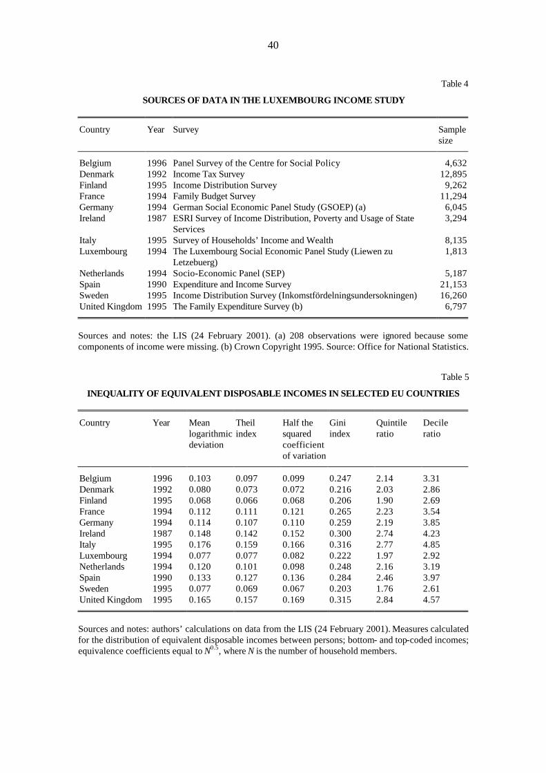
40

Table 4

SOURCES OF DATA IN THE LUXEMBOURG INCOME STUDY

Country Year Survey Sample size

Belgium 1996 Panel Survey of the Centre for Social Policy 4,632 Denmark 1992 Income Tax Survey 12,895 Finland 1995 Income Distribution Survey 9,262 France 1994 Family Budget Survey 11,294 Germany 1994 German Social Economic Panel Study (GSOEP) (a) 6,045 Ireland 1987 ESRI Survey of Income Distribution, Poverty and Usage of State

Services 3,294

Italy 1995 Survey of Households’ Income and Wealth 8,135 Luxembourg 1994 The Luxembourg Social Economic Panel Study (Liewen zu

Letzebuerg) 1,813

Netherlands 1994 Socio-Economic Panel (SEP) 5,187 Spain 1990 Expenditure and Income Survey 21,153 Sweden 1995 Income Distribution Survey (Inkomstfördelningsundersokningen) 16,260 United Kingdom 1995 The Family Expenditure Survey (b) 6,797

Sources and notes: the LIS (24 February 2001). (a) 208 observations were ignored because some components of income were missing. (b) Crown Copyright 1995. Source: Office for National Statistics.

Table 5

INEQUALITY OF EQUIVALENT DISPOSABLE INCOMES IN SELECTED EU COUNTRIES

Country Year Mean logarithmic deviation

Theil index

Half the squared coefficient of variation

Gini index

Quintile ratio

Decile ratio

Belgium 1996 0.103 0.097 0.099 0.247 2.14 3.31 Denmark 1992 0.080 0.073 0.072 0.216 2.03 2.86 Finland 1995 0.068 0.066 0.068 0.206 1.90 2.69 France 1994 0.112 0.111 0.121 0.265 2.23 3.54 Germany 1994 0.114 0.107 0.110 0.259 2.19 3.85 Ireland 1987 0.148 0.142 0.152 0.300 2.74 4.23 Italy 1995 0.176 0.159 0.166 0.316 2.77 4.85 Luxembourg 1994 0.077 0.077 0.082 0.222 1.97 2.92 Netherlands 1994 0.120 0.101 0.098 0.248 2.16 3.19 Spain 1990 0.133 0.127 0.136 0.284 2.46 3.97 Sweden 1995 0.077 0.069 0.067 0.203 1.76 2.61 United Kingdom 1995 0.165 0.157 0.169 0.315 2.84 4.57

Sources and notes: authors’ calculations on data from the LIS (24 February 2001). Measures calculated for the distribution of equivalent disposable incomes between persons; bottom- and top-coded incomes; equivalence coefficients equal to N0.5, where N is the number of household members.

Table 6

DECOMPOSITION OF THE MEAN LOGARITHMIC DEVIATION IN SELECTED EU COUNTRIES

Country Household size Sex of the household head Age class of the household head Household type Total

Within- groups at fixed weights

Between-groups at fixed weights

Demographic effect

Within- groups at fixed weights

Between-groups at fixed weights

Demographic effect

Within- groups at fixed weights

Between-groups at fixed weights

Demographic effect

Within- groups at fixed weights

Between-groups at fixed weights

Demographic effect

value share value share value share value share value share value share value share value share value share value share value share value share

Belgium 0.091 88.4 0.003 3.3 0.009 8.3 0.098 95.5 0.004 4.3 0.000 0.2 0.099 96.0 0.007 6.8 -0.003 -2.8 0.088 85.3 0.008 7.5 0.007 7.2 0.103 Denmark 0.059 74.4 0.005 6.2 0.016 19.5 0.069 86.9 0.008 9.8 0.003 3.4 0.063 79.0 0.013 16.3 0.004 4.7 0.056 69.8 0.013 16.1 0.011 14.0 0.080 Finland 0.058 85.2 0.003 4.5 0.007 10.4 0.062 91.6 0.005 6.8 0.001 1.6 0.062 91.5 0.006 9.1 -0.000 -0.6 0.054 80.1 0.006 9.6 0.007 10.4 0.068 France 0.106 94.1 0.002 2.0 0.004 3.9 0.108 95.9 0.004 3.5 0.001 0.6 0.112 99.6 0.003 2.4 -0.002 -2.0 0.102 90.5 0.006 5.4 0.005 4.1 0.112 Germany 0.108 94.7 0.002 1.7 0.004 3.6 0.109 95.4 0.004 3.2 0.002 1.4 0.110 96.6 0.003 3.0 0.000 0.4 0.102 89.7 0.005 4.8 0.006 5.5 0.114 Ireland 0.151 102.2 0.005 3.3 -0.008 -5.5 0.149 100.6 0.000 0.0 -0.001 -0.6 0.142 96.1 0.004 3.0 0.001 0.9 - - - - - - 0.148 Italy 0.172 98.2 0.003 1.8 - - 0.174 98.9 0.002 1.1 - - 0.172 98.0 0.004 2.0 - - 0.170 96.9 0.005 3.1 - - 0.176 Luxembourg 0.075 97.6 0.001 1.0 0.001 1.4 0.076 98.7 0.001 0.7 0.000 0.6 0.075 97.5 0.002 3.0 -0.000 -0.5 0.072 93.3 0.003 4.2 0.002 2.5 0.077 Netherlands 0.111 92.7 0.003 2.2 0.006 5.1 0.116 96.5 0.004 3.5 0.000 0.0 0.120 99.4 0.003 2.7 -0.003 -2.1 0.104 86.9 0.006 5.4 0.009 7.7 0.120 Spain 0.133 99.8 0.002 1.8 -0.002 -1.6 0.134 100.6 0.001 0.4 -0.001 -1.0 0.131 98.6 0.002 1.6 -0.000 -0.2 0.129 96.9 0.006 4.7 -0.002 -1.6 0.133 Sweden 0.049 63.8 0.004 5.3 0.024 30.8 0.070 90.4 0.005 5.9 0.003 3.7 0.057 74.0 0.007 9.6 0.013 16.4 - - - - - - 0.077 United Kingdom

0.158

96.1

0.004

2.3

0.003

1.6

0.152

92.6

0.010

5.9

0.003

1.5

0.150

91.0

0.010

6.0

0.005

3.0

0.140

85.1

0.016

9.7

0.009

5.2

0.165

Sources and notes: authors’ calculations on data from the LIS (24 February 2001). Measures calculated for the distribution of equivalent disposable incomes between persons; bottom- and top-coded incomes; equivalence coefficients equal to N0.5, where N is the number of household members. “Value” refers to the absolute contribution of the component to the total index; “share” refers to the percentage impact of the same contribution on the total index.

42

Figure 1

INCOME INEQUALITY IN ITALY, 1977-1995

0.09

0.10

0.11

0.12

0.13

0.14

0.15

0.16

0.17

0.18

0.19

1977 1978 1979 1980 1981 1982 1983 1984 1985 1986 1987 1988 1989 1990 1991 1992 1993 1994 1995

0.24

0.25

0.26

0.27

0.28

0.29

0.30

0.31

0.32

0.33

0.34

Mean logarithmic deviation Half the squared coefficient of variationTheil index Gini index (right-hand axis)

Sources and notes: authors’ calculations on data from the SHIW-HA (Version 1.1, October 2000). Measures calculated for the distribution of equivalent disposable incomes between persons, where incomes are net of interest on financial assets; bottom- and top-coded incomes; equivalence coefficients equal to N0.5, where N is the number of household members.

Figure 2

AGE PROFILE OF INCOMES IN ITALY, 1977 AND 1995

0.75

1.00

1.25

Up to 30 years 31 to 40 years 41 to 50 years 51 to 65 years Over 65 years

1977

1995

Sources and notes: authors’ calculations on data from the SHIW-HA (Version 1.1, October 2000). Ratio to the overall mean of the mean equivalent disposable incomes (net of interest on financial assets) of households with heads in the age group indicated; bottom- and top-coded incomes; equivalence coefficients equal to N0.5, where N is the number of household members; households counted as many times as there are members.

43

Figure 3

TOTAL AND WITHIN-GROUP INEQUALITY BY HOUSEHOLD TYPE IN ITALY, 1977-1995

0.09

0.10

0.11

0.12

0.13

0.14

0.15

0.16

0.17

0.18

0.19

1977 1978 1979 1980 1981 1982 1983 1984 1985 1986 1987 1988 1989 1990 1991 1992 1993 1994 1995

Mean logarithmic deviation Within-groups component

Sources and notes: authors’ calculations on data from the SHIW-HA (Version 1.1, October 2000). Measures calculated for the distribution of equivalent disposable incomes between persons, where incomes are net of interest on financial assets; bottom- and top-coded incomes; equivalence coefficients equal to N0.5, where N is the number of household members.

Figure 4

TOTAL AND FIXED-WEIGHT INEQUALITY BY SEX OF THE HOUSEHOLD HEAD IN ITALY, 1977-1995

0.09

0.10

0.11

0.12

0.13

0.14

0.15

0.16

0.17

0.18

0.19

1977 1978 1979 1980 1981 1982 1983 1984 1985 1986 1987 1988 1989 1990 1991 1992 1993 1994 1995

Mean logarithmic deviation Mean logarithmic deviation at fixed weights

Sources and notes: authors’ calculations on data from the SHIW-HA (Version 1.1, October 2000). Measures calculated for the distribution of equivalent disposable incomes between persons, where incomes are net of interest on financial assets; bottom- and top-coded incomes; equivalence coefficients equal to N0.5, where N is the number of household members.

44

Figure 5

TOTAL AND WITHIN-GROUP INEQUALITY BY AREA OF RESIDENCE IN ITALY, 1977-1995

0.09

0.10

0.11

0.12

0.13

0.14

0.15

0.16

0.17

0.18

0.19

1977 1978 1979 1980 1981 1982 1983 1984 1985 1986 1987 1988 1989 1990 1991 1992 1993 1994 1995

Mean logarithmic deviation Within-groups component

Sources and notes: authors’ calculations on data from the SHIW-HA (Version 1.1, October 2000). Measures calculated for the distribution of equivalent disposable incomes between persons, where incomes are net of interest on financial assets; bottom- and top-coded incomes; equivalence coefficients equal to N0.5, where N is the number of household members.

Figure 6

MEAN HOUSEHOLD SIZE IN SELECTED EU COUNTRIES (average number of members)

0.0 0.5 1.0 1.5 2.0 2.5 3.0 3.5 4.0

Ireland

Spain

Italy

Luxembourg

France

Belgium

United Kingdom

Netherlands

Germany

Finland

Denmark

Sweden

Sources and notes: authors’ calculations on data from the LIS (24 February 2001).

45

Figure 7

INCOME INEQUALITY IN SELECTED EU COUNTRIES

0.00 0.03 0.06 0.09 0.12 0.15 0.18

Finland

Sweden

Luxembourg

Denmark

Belgium

France

Germany

Netherlands

Spain

Ireland

United Kingdom

Italy

Mean logarithmic deviation

0.00 0.03 0.06 0.09 0.12 0.15 0.18

Finland

Sweden

Luxembourg

Denmark

Belgium

France

Germany

Netherlands

Spain

Ireland

United Kingdom

Italy

Half the squared coefficient of

variation

0.00 0.03 0.06 0.09 0.12 0.15 0.18

Finland

Sweden

Luxembourg

Denmark

Belgium

France

Germany

Netherlands

Spain

Ireland

United Kingdom

Italy

Theilindex

0.00 0.05 0.10 0.15 0.20 0.25 0.30 0.35

Finland

Sweden

Luxembourg

Denmark

Belgium

France

Germany

Netherlands

Spain

Ireland

United Kingdom

Italy

Giniindex

Sources and notes: authors’ calculations on data from the LIS (24 February 2001). Measures calculated for the distribution of equivalent disposable incomes between persons; bottom- and top-coded incomes; equivalence coefficients equal to N0.5, where N is the number of household members. Countries listed in descending order, from top to the bottom, according to the value of the mean logarithmic deviation.

46

Figure 8

AGE PROFILE OF INCOMES IN SELECTED EU COUNTRIES

0.75

1.00

1.25

Up to 30 years 31 to 40 years 41 to 50 years 51 to 65 years Over 65 years

Italy, 1995France, 1994Germany, 1994Sweden, 1995United Kingdom, 1995

Sources and notes: authors’ calculations on data from the LIS (24 February 2001). Ratio to the overall mean of the mean equivalent disposable incomes of households with heads in the age group indicated; bottom- and top-coded incomes; equivalence coefficients equal to N0.5, where N is the number of household members; households counted as many times as there are members.

47

Figure 9

DEMOGRAPHIC EFFECTS ON INEQUALITY IN SELECTED EU COUNTRIES

-15 -12 -9 -6 -3 0 3 6 9

Finland

Sweden

Luxembourg

Denmark

Belgium

France

Germany

Netherlands

Spain

Ireland

United Kingdom

Householdsize

-15 -12 -9 -6 -3 0 3 6 9

Finland

Sweden

Luxembourg

Denmark

Belgium

France

Germany

Netherlands

Spain

Ireland

United Kingdom

Sex of the household head

-15 -12 -9 -6 -3 0 3 6 9

Finland

Sweden

Luxembourg

Denmark

Belgium

France

Germany

Netherlands

Spain

Ireland

United Kingdom

Age of the household head

-15 -12 -9 -6 -3 0 3 6 9

Finland

Luxembourg

Denmark

Belgium

France

Germany

Netherlands

Spain

United Kingdom

Householdtype

Sources and notes: authors’ calculations on data from the LIS (24 February 2001). Percentage variations in the mean logarithmic deviation obtained by imposing the demographic structure of Italy, expressed as a percentage of the mean logarithmic deviation of Italy. Measures calculated for the distribution of equivalent disposable incomes between persons; bottom- and top-coded incomes; equivalence coefficients equal to N0.5, where N is the number of household members. Countries listed in descending order, from top to the bottom, according to the value of the mean logarithmic deviation.

48

Figure B1 SENSITIVITY OF THE GINI INDEX TO VARIATIONS IN THE PARAMETER ?

OF THE EQUIVALENCE SCALE IN ITALY, 1977 AND 1995

0.29

0.30

0.31

0.32

0.33

0.34

0.35

0.0 0.1 0.2 0.3 0.4 0.5 0.6 0.7 0.8 0.9 1.0

1977distributionbetween persons

1977distribution between households

1995distributionbetween persons 1995

distributionbetween households

Sources and notes: authors’ calculations on data from the SHIW-HA (Version 1.1, October 2000). Indices calculated for the distribution of equivalent disposable incomes, counting each household once (distribution among households), or as many times as it has members (distribution among persons); bottom- and top-coded incomes; equivalence coefficients equal to N?, where N is the number of household members.