TOURISM AND REGIONAL GROWTH IN EUROPE

Raffaele Paci Emanuela Marrocu

WORKING PAPERS

2 0 1 2 / 3 5

C O N T R I B U T I D I R I C E R C A C R E N O S

C E N T R O R I C E R C H E E C O N O M I C H E N O R D S U D ( C R E N O S )

U N I V E R S I T À D I C A G L I A R I U N I V E R S I T À D I S A S S A R I

C R E N O S w a s s e t u p i n 1 9 9 3 w i t h t h e p u r p o s e o f o r g a n i s i n g t h e j o i n t r e s e a r c h e f f o r t o f e c o n o m i s t s f r o m t h e t w o S a r d i n i a n u n i v e r s i t i e s ( C a g l i a r i a n d S a s s a r i ) i n v e s t i g a t i n g d u a l i s m a t t h e i n t e r n a t i o n a l a n d r e g i o n a l l e v e l . C R E N o S ’ p r i m a r y a i m i s t o i m p r o v e k n o w l e d g e o n t h e e c o n o m i c g a p b e t w e e n a r e a s a n d t o p r o v i d e u s e f u l i n f o r m a t i o n f o r p o l i c y i n t e r v e n t i o n . P a r t i c u l a r a t t e n t i o n i s p a i d t o t h e r o l e o f i n s t i t u t i o n s , t e c h n o l o g i c a l p r o g r e s s a n d d i f f u s i o n o f i n n o v a t i o n i n t h e p r o c e s s o f c o n v e r g e n c e o r d i v e r g e n c e b e t w e e n e c o n o m i c a r e a s . T o c a r r y o u t i t s r e s e a r c h , C R E N o S c o l l a b o r a t e s w i t h r e s e a r c h c e n t r e s a n d u n i v e r s i t i e s a t b o t h n a t i o n a l a n d i n t e r n a t i o n a l l e v e l . T h e c e n t r e i s a l s o a c t i v e i n t h e f i e l d o f s c i e n t i f i c d i s s e m i n a t i o n , o r g a n i z i n g c o n f e r e n c e s a n d w o r k s h o p s a l o n g w i t h o t h e r a c t i v i t i e s s u c h a s s e m i n a r s a n d s u m m e r s c h o o l s . C R E N o S c r e a t e s a n d m a n a g e s s e v e r a l d a t a b a s e s o f v a r i o u s s o c i o - e c o n o m i c v a r i a b l e s o n I t a l y a n d S a r d i n i a . A t t h e l o c a l l e v e l , C R E N o S p r o m o t e s a n d p a r t i c i p a t e s t o p r o j e c t s i m p a c t i n g o n t h e m o s t r e l e v a n t i s s u e s i n t h e S a r d i n i a n e c o n o m y , s u c h a s t o u r i s m , e n v i r o n m e n t , t r a n s p o r t s a n d m a c r o e c o n o m i c f o r e c a s t s . w w w . c r e n o s . i t i n f o @ c r e n o s . i t

C R E N O S – C A G L I A R I V I A S A N G I O R G I O 1 2 , I - 0 9 1 0 0 C A G L I A R I , I T A L I A

T E L . + 3 9 - 0 7 0 - 6 7 5 6 4 0 6 ; F A X + 3 9 - 0 7 0 - 6 7 5 6 4 0 2

C R E N O S - S A S S A R I V I A T O R R E T O N D A 3 4 , I - 0 7 1 0 0 S A S S A R I , I T A L I A

T E L . + 3 9 - 0 7 9 - 2 0 1 7 3 0 1 ; F A X + 3 9 - 0 7 9 - 2 0 1 7 3 1 2 T i t l e : TOURISM AND REG IONAL GROWTH IN EUROPE F i r s t Ed i t i on : November 2012 Second Ed i t i on : Oc tobe r 2013

Tourism and regional growth in Europe

Raffaele Paci and Emanuela Marrocu

University of Cagliari, CRENoS

Abstract

The paper analyzes the impact of domestic and international tourism on the economic growth process for 179 European regions. The econometric analysis is based on a spatial growth regression framework where the rate of GDP per capita growth at the regional level for the period 1999-2009 is influenced by tourism flows, in addition to the traditional growth variables. Besides controlling for initial conditions, we also include a wide set of covariates to account for the endowment of human and technological capital and for the geographical, social and institutional features of the regions. The results, confirmed by several robustness checks, demonstrate that regional growth is positively affected by domestic and international tourism. Keywords: regional economic growth; tourism flows; spatial dependence; Europe

JEL: R11, L83, C31

Acknowledgments: The research leading to these results received funding from the Regione Autonoma Sardegna (LR7 2011, Project F71J11000980002). The authors would like to thank Andrea Zara for excellent assistance in preparing the database. We have benefited from valuable comments by participants at the conferences NARSC in Ottawa, IATE in Ljubljana and ERSA in Palermo.

Forthcoming in: Papers in Regional Science

October 2013

   

1

1. Introduction

Tourism represents one of the most relevant and fastest growing industries in the world. The

decrease in travel costs, the rise of large inbound markets such as Russia and China, the increase in

point-to-point flights and the ease of acquiring information on destinations are all elements that

make the tourism sector a significant source of external revenues and a key driver of economic

growth for local economies.

The economic literature has widely analyzed the role of international tourism in the

development process at the country level (Ghali, 1976; Lanza and Pigliaru, 1994; Hazari and Sgro,

1995; Sinclair, 1998). The so-called Tourism-Led Growth (TLG) hypothesis has been investigated

in a number of empirical contributions in cross-country studies at the global level (Sequeira and

Maçãs Nunes, 2008; Lee and Chang, 2008; Figini and Vici, 2010) and in time series analyses of

individual countries in Latin America, Asia and Europe.1 The effectiveness of tourism in driving

economic growth has proven particularly strong for small economies specializing in tourism, such

as several island states (Brau et al., 2007). Regarding European countries in particular, tourism’s

positive role in influencing economic dynamics has been shown by Balaguer and Cantavella-Jordà

(2002) and Capó Parrilla et al. (2007) for Spain, Dritsakis (2004) for Greece and Proença and

Soukiazis (2005) for Portugal. In general, the mechanisms driving the positive relationship between

international tourism and long-run growth are the significant inflows of foreign currency,

stimulation of inter-industry linkages, incentives for public infrastructure investment and the

multiplier effects on employment.2

In the literature cited above, the territorial unit of analysis is the country, and therefore, most

contributions have focused on international tourism flows while neglecting domestic ones because

they do not represent an additional source of external revenue for the nation as a whole. However, it

should be noted that domestic tourists constitute the most important component of total tourism, and

hence, they are expected to considerably influence local economic performance. According to the

World Travel and Tourism Council (WTTC, 2012), domestic tourism flows (i.e., the journeys of

resident tourists within their own countries) represented 70% of total tourism revenues in 2011.

Regarding Europe, in 2010, the number of holiday trips by European Union (EU) residents within

                                                            1 The literature on the relationship between growth and tourism at the country level is extensive and rapidly growing, and unsurprisingly, the results are mixed and inconclusive given the wide range of territorial coverage and methodologies employed. It is outside of the scope of this paper, which focuses on the regional dimension, to provide a comprehensive review. See Brida and Pulina (2010) for a recent survey of the TLG hypothesis and Song et al. (2012) for a general overview of this approach. 2 The literature has recently proposed the so-called TKIG hypothesis (tourism exports, capital goods imports, growth) in which the growth-enhancing effect of tourism may also be channeled through the imports of capital goods acquired thanks to the foreign currency made available by international tourism inflows (Nowak et al., 2007). In our paper, based on a regional framework that includes both domestic and international tourists, it is not possible to distinguish between the TLG and TKIG hypotheses.

2

their own countries surpassed one billion, with domestic tourist flows representing 77% of the total

trips (European Union, 2011).

Therefore, to fully evaluate the role of tourism in economic growth, it is essential to consider

both the domestic and the international tourism flows, and this can only be thoroughly

accomplished when the analysis is conducted at the regional level. For a specific region, say Illes

Baleares, it is irrelevant whether a tourist arrives from another area of Spain, say Madrid or

Barcelona, or from abroad, say Paris or New York. In any of these cases, the arrival of this tourist

represents a source of external revenue for the local economy that improves the regional

performance.3 However, primarily due to a lack of regional data, only two studies thus far have

analyzed the relationship between tourism and economic growth at the regional level: Proença and

Soukiazis (2005) for the regions of Portugal and Cortés-Jiménez (2008) for the Spanish and Italian

regions.4

The aim of this paper is to analyze the influence of domestic and international tourism on

the economic growth rate over the period 1999-2009 for a wide and highly differentiated set of 179

regions belonging to ten European countries: Austria, France, Germany, Greece, Italy, the

Netherlands, Portugal, Spain, Sweden and the United Kingdom. The territorial breakdown is based

on Eurostat’s NUTS (Nomenclature of Territorial Units for Statistics) classification, and we

consider the NUTS2 level, which defines regions as the basic territorial unit for the application of

regional policies.

The econometric analysis is based on a growth regression framework, derived from an

augmented Cobb-Douglas production function (Mankiw et al., 1992), where we specify the regional

rate of per capita GDP growth as a function of tourism flows, as well as the standard right-hand side

growth model variables. We also consider a wide set of controls to account for the geographical,

social and institutional features of the regions.

In contrast to previous contributions, we adopt an empirical approach – based on spatial

econometric techniques – which allows us to properly account for the role of spatial spillovers in

influencing the local growth process. We thus provide original evidence on the crucial issue of

positive externalities acquired from proximate territories.

As a proxy for tourism flows, we consider the number of nights spent in the destination

region by domestic and international tourists. Given the lack of information on the monetary

expenditures of tourists at the regional level, this indicator is more appropriate because it accounts

                                                            3 As is well-known, tourists have different expenditure potential, preferences and interests, and it is important for managers in the destination to differentiate among them. However, on average, a national visitor is as important for the aggregate revenue of the region as an international one. 4 Marrocu and Paci (2011) show that tourism arrivals positively affect the efficiency levels of European regions, as they provide valuable information on the external demand to the local economy.

3

for the length of stay, which varies across regions. However, to check the robustness of our results,

the empirical model is also estimated using the number of arrivals.

The countries considered in this paper are highly representative of the tourism flows of

Europe as a whole, as the tourists’ overnight stays in the ten countries considered amount to more

than 80% of total tourism in the EU. Thus, our analysis provides a wide-ranging and informative

picture of the relationship between tourism and growth because it focuses on countries with varying

degrees of specialization in tourism.

The paper is organized as follows. In section 2, we present the main features of tourism

flows, which constitute our variable of interest in analyzing the regional growth process. In section

3, the empirical framework is discussed in conjunction with certain estimation issues. The

dependent and explanatory variables are presented in section 4. The econometric results of the

baseline model are presented in section 5, while some extensions and robustness checks are

discussed in section 6. Section 7 concludes.

2. Tourism flows in Europe

In this section, we provide a brief overview of our variable of interest, tourism flows, which

are considered an additional driver of economic growth in the European regions. We begin by

analyzing the main figures at the country level and then examine the regional patterns in greater

detail. It is important to note that our set of countries is highly differentiated, as it comprises highly

developed and industrialized nations, such as Germany and France, and small, relatively less

developed countries where the tourism sector plays a significant role, such as Greece and Portugal.

Moreover, the set of regions considered includes widely renowned tourism destinations, such as

national capitals (Paris, London, Rome, Berlin and Madrid), cultural cities (Venice, Florence and

Barcelona), top “sea & sun” destinations (Illes Baleares, Sardegna, Algarve, Andalucia and the

Greek Islands) and mountains destinations in the Alps (Bozen, Tirol, Rhône Alpes). Moreover, our

sample includes several other regions, both fast and slow growing, where tourism is not particularly

developed. Such high sample variability is important to correctly assess the role of tourism in

influencing economic performance in the overall economy.

In Table 1, we report the number of overnight stays by domestic (which also include intra-

regional flows) and international tourists in the initial and final years of the period 1999-2009. The

number of visitors’ overnight stays is the most general indicator of tourism flows because it also

accounts for the length of the stay. Overall, the total number of nights spent by tourists in the ten

countries in 2009 amounts to 1.8 billion, and the domestic component accounts for the highest share

(62%), which is quite stable over the decade.

4

The country with the largest tourism flow is Italy (370 million in 2009), followed by

Germany (314) and France (290). It is evident from these sizeable values that tourism has an

important impact on economic activity. For instance, the WTTC (2011) estimates that in Italy in

2009, the tourism sector directly generated revenues of 50 billion euro (3% of GDP), which

increase to 130 billion (8% of GDP) when the indirect and induced effects are also included.

The composition of total tourism flows is strongly differentiated among countries: the

domestic share ranges from a very low level in Greece (29%) and Austria (30%) to a very high level

in Sweden (76%) and Germany (83%), while Italy and Spain exhibit a more balanced composition

between domestic and international tourist flows.

To fully appreciate the relevance of the different compositions of tourist flows, it is

important to note that, according to international definitions (United Nations World Tourism

Organization, Eurostat), a “tourist” is defined as a person who spends at least one night in official

tourist accommodation establishments.5 Moreover, the official statistics do not permit

distinguishing between business and leisure tourists.6 In wealthy and populous European countries,

such as Germany or the United Kingdom, the higher share of domestic tourism can be partly

explained by the presence of a large business component.7 Table 1 also reports the dynamics of

tourism nights over the last decade, which witnessed an overall annual average growth rate equal to

1.4% for the domestic component and 1.6% for the international one. Again, there is substantial

variability among countries and components. The highest growth rates are observed for domestic

tourism in Spain (5.2%) and Greece (3.9%), due to the improved economic conditions registered in

that period in these two countries. International tourism experienced a substantial increase in

Germany (4%) and Spain (3.4%), while the Netherlands and Portugal reported small declines.

In Map 1 and Map 2, we depict the regional distribution of overnight tourism stays for the

domestic and international components for the year 2009, while the top ten regions are listed in

Table 2. A visual inspection of the maps reveals that both domestic and international tourism flows

exhibit a well-defined geographical pattern. To formally test for the presence of spatial association

in the regional distribution of tourists, we conducted Moran’s I test using the inverse of the distance

between any pair of regions in kilometers as the spatial weight matrix. The results of Moran’s I test,

equal to 3.65 for domestic flows and to 4.28 for the international ones, are highly statistically                                                             5 The available data do not include tourists staying in relatives’ or friends’ houses. Therefore, the effects of tourism flows on regional performance may be underestimated. 6 According to WTTC (2012), the leisure component accounts for 78% of total tourism revenues in the European Union. 7 The WTTC (2012) reports that countries with high shares of business tourism in GDP also present high shares of domestic tourism in GDP. For instance, Germany exhibits high values for both shares (38% and 63%, respectively) and the same is true in the United Kingdom (36% and 69%); however, Greece (6% and 45%) and Portugal (13% and 36%) present low values for both indicators. Overall, the cross-country correlation between business and domestic tourism (in GDP) is equal to 0.53.

5

significant in both cases. This means that tourism destinations are spatially associated, which may

be the result of the presence of natural elements (such as being on coasts or in the mountains) but

may also be due to communication processes activated by previous tourist flows, which can

generate positive externalities. This type of cross-regional correlation is likely to affect the

relationship between growth and tourism and hence the empirical analysis is performed within a

spatial econometric framework.

Two interesting results emerge regarding the regional ranking of tourism destinations. First,

there are remarkable differences between the domestic and international rankings. Some

destinations clearly specialize in internal tourism, such as Emilia Romagna in Italy, Mecklenburg in

Germany, Dorset and Somerset in the UK or Provence in France. Other regions only appear among

the top destinations for international tourism, such as Illes Balears (which is the most attractive

destination in Europe, with 48 million nights spent in 2009), London and the Italian region of Lazio,

where Rome is located. Few areas are able to be highly attractive for both domestic and

international tourists: Île de France for the world-renowned destination of Paris and other regions

(Cataluña, Veneto, Toscana and Andalucía) that combine the attractiveness of cultural cities

(Barcelona, Venice, Florence and Seville) with the “sea & sun” holiday product.

The second result refers to the high variability in the tourism destinations with respect to the

growth rates of domestic and international tourism over the period 1999-2009. The strong

competition among destinations has induced several changes in the rankings, especially for

domestic tourism. A relevant example of these remarkable changes in tourism destinations is

provided by traditional coastal destinations around Wales in the UK, where we observe the highest

reduction in domestic tourism in Europe: East Wales (-7.4% annual average change over the 1999-

2009 decade) and Dorset and Somerset (-3.4%), accompanied by a substantial increase in nearby

alternative destinations, such as West Wales (10.8%) and Gloucestershire (9.6%). Moreover, the

dynamics of the international component of tourism are also highly variable: among the most

popular destinations, some have very positive performances, such as Berlin (18.7% annual average)

and Sardegna (10.2%), which stand in sharp contrast to the remarkable decline experienced by other

destinations, such as Algarve (-2.1%) and Bretagne (-2%).

Map 3 displays the share of the domestic component in total tourism at the regional level in

2009. As mentioned above, there are regions that almost entirely specialize in domestic tourism,

such as Mecklenburg in Germany, where a substantial share of total tourism flows (25 million

nights) is composed by domestic tourists (97%). Similar figures are found for other German regions

because of the significant number of domestic flows represented by business trips. The changes in

certain UK destinations, such as Cornwall (domestic share equal to 94%) and Dorset (92%), are

6

more related to the presence of traditional domestic leisure tourism. Conversely, there are popular

destinations where the share of domestic tourism is very low, such as the Austrian mountain

destination of Tirol (9%) or the islands of Kriti (9%) in Greece and Illes Balears (13%) in Spain.

Finally, in Map 4, we report the pattern of regional specialization in the tourism sector. The

specialization index is computed from a supply side perspective as the regional share of beds

available in tourist accommodation establishments relative to the regional GDP share.8 This index

of comparative advantage takes a value above 1 if the region is relatively specialized in tourism

activities and below 1 if it is not specialized. Among the highly specialized tourism regions, we find

several islands in Greece (Notio Aigaio, Ionia Nisia, Kriti), Spain (Illes Balears), France (Corse),

Italy (Sardegna) and a coastal region of Portugal (Algarve), which are essentially summer

destinations for “sea & sun” holidays. We also observe small mountain regions in the Alps

(Bolzano, Trento, Valle d’Aosta, Tirol, Karnten) that are attractive destinations in both winter and

summer. From the visual inspection of Map 4, it is clear that regions specializing in tourism (the 83

regions in the highest two classes) show a high degree of spatial correlation, as most regions’

specialization in tourism activities is determined by common geographical features such as being

located on the coast or in the mountains. Finally, the regions specializing in tourism are also

characterized by relatively lower levels of per capita GDP, but exhibit higher growth rates (0.37%)

with respect to the other regions (-0.03).

It is important to note that our sample includes several regions where the tourism industry is

very small compared to other economic activities. This regional variability is essential to ensure that

the econometric analysis can assess the role of tourism in regional economic performance, not only

in areas specializing in tourism, but more generally in the full set of European regions.

3. The empirical framework

3.1 Estimation issues

Tourism’s role in regional economic dynamics is analyzed using a growth model derived

from a human capital augmented Cobb-Douglas aggregate production function à la Mankiw-

Romer-Weil (1992). In addition to the standard right-hand side variables included in traditional

growth models, we also explicitly consider tourism flows as an additional potential driver of local

economic performance and a set of controls at both the regional and national levels. As is widely

recognized by economic growth scholars, there is no consensus in the empirical growth literature on

                                                            8 We also computed the tourism specialization index using employment in the “Hotel, restaurant and bar” sector. However, this measure was inadequate because of the high incidence of restaurant and bar activities that in certain regions (as is the case for pubs in the UK) primarily serve local residents rather than external consumers, and hence may not be directly associated with tourism.

7

which determinants should be included in a statistical model. Brock and Durlauf (2001) note that

growth theories are “open-ended”, as most of them are compatible, rather than mutually exclusive,

meaning that the roles different factors play in the growth process can be investigated in a single

model. In this study, we thus contribute to the current debate on the possible drivers of economic

growth by analyzing whether tourism activities enhance our understanding of regional economic

development while accounting for the documented role of institutional and geographical factors.

It is important to note that the evidence provided in this study, as is also the case in most

empirical growth analysis, has to be interpreted with caution. As emphasized by Durlauf et al.

(2009), in growth analysis it is extremely difficult to identify proper causal effects because genuine

sources of exogenous variability are very rare; almost every socio-economic factor can have an

effect on growth and can in turn be influenced by growth. However, the analysis of income

dynamics is valuable because it contributes to revealing (or ruling out) important correlations

between growth and different economic factors.

The estimation of growth models at the regional scale entails addressing two important

methodological issues. The first relates to the endogeneity of the regressors, and the second

concerns cross-sectional dependence; as the observation units are regions, they typically exhibit

significant spatial association. In the case of empirical growth models, the two issues are inherently

intertwined, and a unique framework is required to address them both. The non-spatial empirical

literature on economic growth has primarily focused on endogeneity issues, while spatial matters

were simply addressed by including additional variables with geographical content (Durlauf et al.,

2009). Therefore, most attention has been devoted to the question of how to address endogeneity

problems, which may be caused by a number of different sources, namely, unobservable

heterogeneity, measurement errors and reverse causality. One of the most effective approaches to

address the endogeneity issue is based on the panel version of the Generalized Method of Moments

(GMM) (Arellano and Bond, 1991; Blundell and Bond, 1998), which has been widely applied in

empirical studies, including those related to the analysis of the relationship between growth and

tourism (see, among others, Cortés-Jiménez, 2008; Seetanah, 2011). However, the GMM method

requires the model to satisfy a potentially large number of moment conditions and, most important

for a regional level analysis, it is derived under the assumption that the error term cannot be

correlated across units. Therefore, such an assumption is rarely satisfied in the case of regional data

due to the likely presence of spatial correlation9, which must be properly addressed. For this reason,

                                                            9 Note that the issue of spatial correlation has been neglected in previous studies conducted at the country level, despite that most countries specializing in tourism are spatially clustered due to geographical first nature conditions, and therefore, the results provided are likely to be affected by omitted variable bias.

8

differently from other recent contributions in tourism economics, we adopt an empirical approach

that enables us to simultaneously account for endogeneity and spatial correlation.

At the regional level, spatial correlation is often the result of the spillovers generated by the

interactions among agents, firms and institutions. The existence of positive externalities leads to the

concentration of economic activities in particular areas, where inputs are made more productive,

yielding increasing returns to scale and growth effects, as predicted by new economic geography

models and endogenous growth theory (Romer, 1986). However, the role of spatial spillovers in

determining diversified growth paths and varying speeds of convergence has generally been

overlooked in non-spatial growth empirics. Since the publication of the US regional convergence

study by Rey and Montouri (1999), spatial models have been adopted to investigate regional growth

issues. As emphasized by Abreu et al. (2005) and Fingleton and López-Bazo (2006), spatial

dependence in long-run growth rates is primarily due to substantive economic mechanisms (factor

mobility, knowledge diffusion and pecuniary externalities), the economic underpinnings of which

have been analyzed in depth by agglomeration and economic geography scholars (Ottaviano and

Thisse, 2004).

In our analysis, we address the spatial association issue by augmenting the standard growth

model with regressors featuring spatial patterns and we deal with the endogeneity problem by

including the explanatory variables lagged by five periods. This lag is expected to eliminate the

possible correlation between the error term and the regressors. As a robustness check, our main

results are contrasted with a cross-sectional growth model, where the explanatory variables are

included with a ten-year lag to further reduce potential endogeneity.

3.2 The empirical model

The empirical model that accounts for both endogeneity and spatial features is specified in

per capita log-linearized form as follows:

ttitjjtitititititti

CDXSFhkktourismyyti _;,,4,3,2,1_; ,

(1)

where i=1, …, 179 regions, t=2004 and 2009, =5, j=1,…, 10 countries and is the error term.

Our sample comprises regional observations for the period 1999-2009. The dependent variable ( y )

is the annual average rate of per capita GDP growth, computed over two five-year periods, 1999-

2004 and 2004-2009. This procedure, standard in the empirical growth literature (Islam, 1995;

Temple 1999), enables us to avoid the undue influence of business cycle fluctuations, which would

9

be reflected in year-on-year growth rates, and detect medium-to-long term growth patterns. Model

(1) above is estimated by pooling the resulting observations for the two periods for the 179 regions.

Following the standard approach employed to estimate growth models (Durlauf et al. 2009),

the right-hand side variables are included in the model lagged at their initial period values; in our

case, this entails a five-year lag (=5). Such a lag allows us to consider a period long enough for the

explanatory variables to exert their effects on the growth rate and reduce the potential problem of

endogeneity due to simultaneous reverse causality. In addition to the number of nights of tourism

stays (tourism), we include the initial period’s level of per capita GDP (y) to control for

convergence and catch-up dynamics and the traditional production inputs of physical capital stock

(k) and human capital (hk).10

To account for the existence of proximity externalities, we also include spatial factors (SF)

selected on the basis of the model specification, which will be discussed in detail in section 5.

Moreover, we include a set of regional controls gathered in the matrix X, a set of time invariant

dummies for the 10 countries (CD) considered in this study and, finally, time dummies () to

account for common shocks. The regional controls comprise the demographic and settlement

structure, the endowments of technological and social capital, the degree of cultural diversity and

first nature factors.11

4. Variables and data description

In this section, we provide detailed definitions of the variables considered in the estimation

model, as well as a brief description of their main characteristics. For the sake of simplicity, the

summary statistics presented in Table 3 refer to the whole period considered, 1999-2009; the

detailed definitions and sources of the variables are reported in Appendix 1.

Our dependent variable is the annual average rate of real per capita GDP growth, which

exhibits highly differentiated dynamics across regions, ranging from the minimum negative value of

-2.6% in the Austrian region of Vorarlberg to the maximum of 4.4% in Attiki (Greece). The high

variability in the per capita GDP growth rate is also indicated by the coefficient of variation, which

exhibits the highest value of all of the variables.

Following a well-established literature (refer, among others, to Abramovitz 1986, Barro and

Sala-i-Martin, 1991), we include the initial level of per capita GDP in the growth model, which is

                                                            10 Because all variables are included in per capita terms, the labor input is omitted. 11 Ideally, we should also include a measure of the degree of openness of the region among the explanatory variables; unfortunately, data on trade at the regional level are not available for Europe. The inclusion of the country dummies may account for the omission of variables, such as the degree of openness, as long as they are primarily characterized by national patterns.

10

expected to have a negative sign in the presence of a regional convergence process, and physical

and human capital as main production inputs.

Our variable of interest, discussed in detail in section 2, is represented by tourism flows

measured by the number of overnight stays, of which we consider both the domestic and

international components. As argued previously, this variable is preferred to the number of arrivals,

as it allows for a more thorough assessment of the contribution of tourism activities to overall

economic performance. However, to check the robustness of our results, we also estimate the

preferred model specification by including tourism flows measured in terms of arrivals.

The total stock of physical capital is calculated for each region by applying, over a long

period beginning in the 1985, the perpetual inventory method based on gross investment in the

previous year and assuming an annual depreciation rate of 10%.12 This is a general measure that

includes both private and public capital stocks.

The human capital variable accounts for the accumulation of intangible knowledge, which

has been demonstrated to significantly affect economic dynamics at both the country (Benhabib and

Spiegel, 1994) and regional levels (Dettori et al., 2012). Our human capital indicator is expressed as

the number of economically active individuals (in thousands) that have attained at least a tertiary

education degree (ISCED 5-6). Mankiw et al. (1992) show that in the augmented formulation of the

Solow growth model, human capital can be included either in terms of accumulation or in levels. In

this paper, we prefer to employ the stock notion of human capital because, in contrast to measures

such as enrolment rates13, it accounts for the contribution to the economy provided by active

individuals who have attained the highest levels of education. Moreover, this variable is also

supposed to account for the heterogeneity in efficiency growth across regions (Marrocu and Paci,

2013a). Note that this approach has been followed in previous contributions in regional economics

(Rodriguéz-Pose and Crescenzi, 2008; Sterlacchini, 2008; Fisher et al., 2009).

The literature has shown that the growth process may also be influenced by other factors that

characterize the local environment, and thus, we include them in the general specification of our

model. These additional factors can be broadly divided into tangible and intangible assets. The

latter, which usually include technological capital, social capital, education and creativity, have

been found to exert a positive effect on local economic dynamics. On the other hand, tangible assets

                                                            12 In a preliminary analysis, we also considered a specification that included the investment rate in place of the capital stock, but it was not significant; we thus prefer to include the capital stock, which is also intended to control for possible heterogeneity in the initial level of technology and the steady-state position toward which the regions are converging. The overall evidence is robust to the inclusion of either investment or the stock of capital; the results are available from the authors upon request. 13 Note also that the Eurostat series on student enrolments at different educational levels have several missing data, while the Eurostat data on the level of human capital is complete and more reliable as it is retrieved from the Labor Force Survey.

11

(population density, infrastructure and physical capital) may have both positive or adverse effects

on economic growth. Depending on the territorial characteristics of the local economies, negative

influences may arise as the result of congestion or crowding out effects.

The first factor considered refers to the demographic structure of the regions, and this is

usually proxied by population density (computed as the resident population per square kilometer).

However, to account for the high territorial heterogeneity across the European regions, in this study

we prefer a more complex index of the regional settlement structure, which is a discrete variable

that defines six groups of regions according to both population density and city size. The resulting

territorial hierarchy thus comprises regions with the least densely populated areas without urban

centers, for which the index takes a value of one, up to regions with very densely populated areas

and large cities, for which the index assumes the maximum value of six. Given its piecewise nature,

this variable is considered more appropriate for capturing possible nonlinearities in population

density. We expect a positive correlation with the growth rate because a high concentration of

people implies greater local demand and a wider supply of local public services, which are expected

to enhance firms’ productivity growth (Ciccone and Hall, 1996).

The second factor is technological capital that may be considered, at least partially, a public

good generating external spillovers (Griliches, 1979). Therefore, firms located in areas with intense

technological activities exhibit greater productivity growth, and this in turn is expected to increase

the performance of the entire local economy. Following a well-established literature (Griliches,

1990), we employ the number of patent applications presented to the European Patent Office by

inventors resident in the considered regions as the indicator for technological capital.14

The economic performance of a region may also be influenced by its degree of social capital

– a complex mixture of shared norms, ties and trust – which is expected to improve the economic

growth of the local community by decreasing transaction costs and facilitating coordination among

agents (Knack and Keefer, 1997). It is difficult to measure a complex and informal phenomenon

such as social capital (Glaeser et al., 2002), and several indicators have been employed in empirical

studies. In this paper, we employ the level of general trust as a proxy for regional social capital (La

Porta et al., 1997), which has been shown to positively affect the economic performance of

European regions (Marrocu and Paci, 2013a). More precisely, we use the share of the population

who report believing that individuals are helpful, as reported by the European Social Survey.15

                                                            14 Patent counts have the advantage of providing a long time span along with large regional and sectoral coverage; moreover, it has been proved that they are closely correlated with other measures of technology, like research and development expenditures and new products (Acs et al. 2002). 15 Note that such indicator is time-invariant and for Germany, France and the United Kingdom it is available only at the NUTS1 level (macro-regions); therefore, we assume the same value for all NUTS2 regions included in the corresponding NUTS1 macro-region.

12

Another variable related to the concept of social capital is the level of tolerance, which

signals the presence of an open society able to accept external population, attract innovative firms

and highly educated and skilled people, who ultimately are expected to enhance economic

performance (Florida, 2002). As a measure of tolerance, we compute the share of population that

has not mentioned the item “don’t like as neighbors: immigrants/foreign workers” as a response in

the European Value Studies (EVS) questionnaire. Moreover, following the traditional approach in

empirical studies of growth since the seminal work by Barro and Sala-i-Martin (1991), we control

for the possible influences of geographic first nature factors. More specifically, we include a climate

indicator, proxied by the annual average temperature, which is expected to have a negative effect on

regional performance. Finally, we include a full set of country dummies to control for institutional

characteristics, common to regions belonging to the same state, and unobservable heterogeneity at

the national level.

5. Econometric analysis

5.1 Model specification

Based on the discussion presented in the previous sections on the relevance of externalities

generated by proximate regions, the first step of our estimation strategy involves selecting a model

specification that properly accounts for substantive spatial dependence. In this case, the candidate

models are the cross-regressive model, which entails the inclusion of spatial lags for the explanatory

variable supposed to channel the external effects; the spatial autoregressive model, which includes

the spatial lag of the dependent variable; and the spatial Durbin model, which requires the inclusion

of spatial lags for the dependent and independent regressors. The first specification implies the

existence of local spillovers, while for the other two specifications spillovers are global because

they are propagated throughout the system of regional units through a complex structure of

interactions (Anselin, 2003 and 2010).

In our study we first investigate whether our data is consistent with the existence of global

spillovers by estimating the spatial autoregressive specification and spatial Durbin one. Following

the traditional specification approach in spatial econometrics, in the first stage of our analysis we

estimate the non-spatial version (the SP term is excluded) of model (1) by applying the Generalized

Least Squares (GLS) method and then we test the residuals for spatial dependence by applying the

robust version of the Lagrange Multiplier (LM) tests. These are devised to detect either the

existence of spatially correlated errors (spatial error) or the omission of a spatially lagged dependent

variable (spatial lag). In performing the tests, we employ a weighting matrix whose entries are

13

inversely related to the bilateral geographical distance for each pair of regions (in kilometers)16. The

estimated model is reported in the first column of Table 4. Spatial random shocks are not found to

be relevant,17 as only the spatial lag test is significant at the 10% level. However, estimation of the

spatial autoregressive model resulted in a non-significant coefficient for the spatially lagged

dependent variable and non-significant spillover effects. The spatial Durbin model yielded similar

results, which are likely due to the very complex externalities structure implied by such

specification that puts too strong a requirement on the data, especially at the territorial level

considered in this paper (NUTS 2 regions). The interpretation of these findings is that our data are

not compatible with the existence of global spillovers. Following Anselin (2003, 2010), Fingleton

and López-Bazo (2006) and recent methodological development in spatial econometrics (Elhorst,

2010 and Halleck Vega and Elhorst, 2013), we thus consider the cross-regressive specification

based on the inclusion of spatial lags for the initial levels of the per capita GDP, physical capital,

human capital and tourism flows. The relevance of the initial income level is directly linked to the

existence of agglomeration and knowledge diffusion effects, as are broadly documented by new

economic geography models and endogenous growth theory. The spatial lags of both physical

capital and human capital were not found to be significant; this result may be because the

externality effects they induce are already accounted for by the more comprehensive per capita

GDP spatial lag.18 Conversely, the spatial lag of tourism overnight stays was highly significant,

indicating that the high degree of spatial correlation exhibited by inter-regional tourism flows (De la

Mata and Llano-Verduras, 2012; Marrocu and Paci, 2013b) has predictive power with respect to

growth performance. Such correlation in tourism flows is induced by interactions among visitors

and tourist operators at both the origin and destination locations,19 which can activate another

source of production externalities yielding positive growth effects.

The model estimated with the additional spatial regressors does not exhibit any evidence of

remaining residual spatial correlation, as indicated by the LM test reported at the bottom of column

(2) in Table 4. For this model specification, which is the most general one, some control variables

were not significant; this is the case for technological capital, social capital, cultural diversity and

climate. For some of these, we also consider alternative indicators, but they did not exhibit higher

                                                            16 Following the recommendations in Kelejian and Prucha (2010) the weight matrix is max-eigenvalue normalized. 17 This result is consistent with the arguments in Fingleton and López-Bazo (2006) who state that random shocks, which imply a spatial autoregressive process for the error term, play a secondary role in the case of growth processes. 18 Another possible explanation is that their effects can only be detected at a finer regional scale. 19 This type of spatial dependence is the result of learning (at destination locations) and communication (at the origin) processes as tourists share their travel experiences within their networks of family and friends. Locations adjacent to a visited destination are usually visited during the same holiday or become the destinations for future trips. Moreover, recommendations of visited destinations spreads around the tourists’ areas of origin, by decreasing the uncertainty for potential visitors regarding that specific place and increasing the propensity to travel to that destination among consumers in the contiguous areas, they induce origin dependence (Yoon and Uysal, 2005).

14

significance levels. For technological capital the alternative proxy was the stock (rather than the

flow) of patents cumulated over the last five years or the share of R&D expenditures in GDP. For

cultural diversity, we also consider the percentage of foreign born-population. The non-significant

results for some control variables may be due to the quality of the data; the proxies currently

available for a large set of regions considered at the NUTS2 level may be not sufficiently accurate

to describe complex phenomena such as social capital or cultural diversity.20 However, as such

factors are highly persistent, it could also be the case that their effects are, at least in part, accounted

for by the initial level of per capita GDP and by its spatial counterpart term.21

For parsimony, our preferred specification excludes the non-significant control variables and

hence the estimated model reported in the third column of Table 4 represents the starting point of

the investigation on the contribution of tourism activities to regional economic growth.

5.2 Baseline model results

In the model reported in the last column of Table 4, the tourism variable, measured in terms

of overnight stays, exhibits a significant and positive coefficient (0.27), indicating that the growth

rate of regional income per capita is notably correlated with hospitality activities. The latter, if we

cautiously rely on a causal interpretation of the estimated parameter, could be considered a relevant

additional source of economic growth, especially for territories that do not have a comparative

advantage in other types of production but are endowed with natural or cultural resources. We will

address this issue in greater depth in section 6.1, where we discuss the evidence obtained for regions

that specialize in tourism activities. The effect of tourism is strongly enhanced by the flows of

visitors recorded in nearby areas, as the significant coefficient of the spatially lagged term is

estimated at 3.65. This signals the relevance of the positive externalities occurring due to the flows

of information associated with individuals’ journeys, which can activate further tourist flows and

increase the demand for the products experienced at the destination sites (Marrocu and Paci, 2011;

Brau and Pinna, 2013).

Focusing on the other results, we found that the coefficient of the initial level of per capita

GDP, negative and highly significant, is consistent with the prediction of convergence and catching-

up models. Its spatially lagged counterpart is also highly significant, with a positive and sizeable

coefficient (1.23). This indicates the importance of being located within a wealthy area, where there

                                                            20 In order to check whether the results are due to high multicollinearity among the control variables included in model 2 of Table 4, we have computed the Variance Inflation Factors (VIF) for the whole set of controls. They turned out to be well below the threshold value of 5 (the only exception being the technological capital with a VIF of 7), indicating that multicollinearity is not an issue in our estimated model. 21 A complementary explanation may relate to the fact that such variables might have a positive effect on the level rather than the growth rate of GDP (Dettori et al., 2012).

15

is significant potential to acquire the beneficial effects of agglomeration and knowledge diffusion,

ultimately resulting in enhanced income dynamics. This result is reinforced for the regions that rank

in the highest positions of the territorial hierarchy, as is demonstrated by the positive and significant

coefficient of the settlement structure typology variable. Densely populated regions with large

centers are likely to attract the most innovative, high value-added type of productions, and they are

thus expected to exhibit more rapid growth.22

As emphasized by the substantial empirical growth literature initiated by the seminal paper

by Mankiw et al. (1992), human capital represents a highly relevant driver of economic growth; in

our estimated model, it exhibits a significant and sizeable effect of 1.04. Highly educated

individuals, especially those specializing in science and high-tech fields, tend to concentrate in large

urban centers, where they play a crucial role in developing or enhancing the innovative productions

discussed above (Marrocu and Paci, 2012). Finally, the stock of physical capital does not turn out to

significantly affect regional growth performance. The non-significant results for both physical and

technological capital may be because, as we mainly consider the most advanced economies in

Europe, they are likely to only have level effects and not additional growth ones. The latter, as

noted in the discussion above, are primarily determined by intangible factors or particular activities,

as is the case for tourism, which are increasingly characterized by high degrees of innovativeness

and high-tech services to meet the increasingly demanding preferences of heterogeneous

consumers.

5.3 Tourism components

Although the two components of tourism - domestic and international - are inherently

associated (they exhibit a significant correlation coefficient of 0.43) because they are driven by the

same fundamentals (e.g. the degree of attractiveness of a given region), we have also investigated

whether some insights can be provided on their possible different effects on the local economic

growth performance.

In order to avoid multicollinearity problems, in the models reported in columns (1) and (2)

of Table 5 the two tourism components are included one at time.23 The main result is that the

domestic component is a more effective (0.30) indicator of the role hospitality activities play in

economic growth than the international one (0.20). As discussed in the second section, the domestic

component represents, on average, more than 60% of total overnight stays by tourists and exhibits a

                                                            22 Similar results were found when we included the simple population density variable. 23 Moreover, when they are both included in the same empirical model, the high standard errors yielded non-significant t-statistics for both components. The identification of the effect exerted by each component would require another estimation framework, one based on the specification of a simultaneous system that also accounts for the structural links between the two tourism components. However, this type of analysis is beyond the scope of this study.

16

more stable pattern over time when compared to international tourists. The higher coefficient

associated with the domestic tourists may be reasonable due to the fact that the domestic component

also includes intra-regional overnight stays: at a finer spatial scale (provinces or municipalities)

intra-regional flows may activate the same kind of positive externalities discussed for the baseline

model.

It is noteworthy that the domestic component is associated with a sizeable effect due to

tourists visiting contiguous regions. This result can be attributed to the intensity of information and

knowledge flows that occur within the same country, and it is reasonable to argue that they are

facilitated by common norms and beliefs and the absence of language barriers. In the case of the

international component, the same term is not significant because interactions among international

tourists are likely to be much more loose and volatile.

Additional growth effects are observed for tourists visiting regions in which the national

capital city is located (specification 3 of Table 5 where, to save space, we only report the results of

model that includes total tourist nights). This positive result (0.82), primarily driven by international

tourists, is due to the European capital cities being the urban centers with the greatest historical,

artistic and cultural heritage in the world, where world-renowned museums, famous churches and

unique buildings (for instance, the Coliseum in Rome or the Acropolis in Athens) are located.

Finally, note that for all the three models reported in Table 5, the evidence previously discussed on

the determinants of regional growth other than tourism is confirmed. The only exception is the

settlement typology index, which is no longer significant in model 3. This is likely because its effect

is now subsumed by that exerted by the interaction term represented by the nights spent by tourists

in regions with the capital city. These regions exhibit the highest values for the settlement typology

index, eight regions out of ten take the maximum value of six and the other two (Stockholm and

Lisbon) a value of five.

The evidence provided by the last model in Table 5 indicates that tourism may play different

roles in economic growth depending on the characteristics of the territories. Therefore, in the next

section, we propose a deeper investigation of this issue by extending the analysis and focusing on

regional tourism specialization.

6. Model extensions and robustness analysis

6.1 Tourism specialization

To examine the different growth-enhancing effects of tourism, we perform a subsample

analysis. We thus distinguish between regions exhibiting productive specialization in hospitality

activities and regions specializing in other economic activities. Regions exhibiting a value of the

17

tourism specialization index greater than 1.05 belong to the first group, which thus comprises 83

regions.24 As explained in section 2, the specialization index is measured in terms of the regional

share of beds available in tourist accommodation establishments relative to the regional share of

GDP.25 The regions specialized in tourism have been depicted in the two highest classes of Map 4

and comprise several islands and coastal regions and also small mountain regions in the Alps. The

results in Table 6 are reported for both regions specializing in tourism and those that do not. The

tourism coefficient for the first group is sizeable and highly significant, while for the second group

significance is only obtained at the 16% level. It is worth noting that the tourism estimate obtained

for the specialized regions is more than twice that observed for the full sample of regions (0.79 vs.

0.27).26 The results reported for model 1 in Table 6 also confirm the relevance of tourism overnight

stays spent in neighboring regions; note that the spatial lag term is computed with respect to all

other regions, regardless of whether they specialize in tourism. It is interesting to note that the

spatial lag of the tourism variable is also large in magnitude and significant in the case of the

relatively non-specialized regions. This result seems to confirm the relevance of knowledge and

information conveyed by tourists, which are spread beyond specialized territories and are effective

in activating externalities beneficial to the growth process. These may be realized directly by

tourists’ day trips to locations close to their initial destinations or indirectly by increasing the

production of goods and services demanded by proximate regions specializing in hospitality

activities, as well as by the sharing of large sized infrastructures (ports, airports, conference and

exhibition centers) which induce the emergence of territorial clusters.

It is important to highlight that regions highly specialized in tourism activities are on

average characterized by lower levels of GDP per capita with respect to the full sample. This is

reflected in the coefficient of the initial level of per capita GDP, which is much lower with respect

to the estimates reported in the previous tables for the full sample. Moreover, less wealthy regions

are often surrounded by regions with similar per capita income levels due to historically

unfavorable agglomeration patterns, which have ruled out long-run growth types of specialization

such as those related to high-tech production. In our estimated models, this is indicated by the non-

significant coefficients of the spatial lag of the initial level of per capita GDP and the settlement

                                                            24 We have preferred to set 1.05 as cut-off point to exclude those regions that are very close the “neutral” value of 1. Indeed in the range 1-1.05 there are only 5 regions and even if we include them among our sample of specialized regions the estimation results do not change. 25 We also computed the index of relative specialization in terms of population rather than GDP. The estimation results are very similar given the high correlation coefficient (0.96) between the two measures of relative specialization. This confirms that our preferred indicator of specialization is robust to rescaling methods. 26 Similar results, not reported to save space, were also found when conducting the analysis by considering the domestic and international components of tourism nights.

18

structure variable. Note that human capital is also found to be less growth enhancing for regions

specializing in tourism.

The subsequent model results presented in Table 6 provide further evidence that tourism

may have differentiated effects according to certain regional characteristics. The results reported for

models 3 and 4 refer to the subsample of regions highly intensive in international tourism (45)27 and

the group of regions (90) with coastal territories, which are presumed to have a natural comparative

advantage in attracting tourists. In both cases, the results indicate that tourism has a greater effect on

growth than that reported by the baseline model; the coefficient on total tourism overnight stays is

estimated at 0.48 and 0.35 for highly international tourism intensive regions and coastal regions,

respectively. Conversely, this coefficient is substantially lower than that found for regions

specializing in the tourism sector (model 1). The relevance of this specialization is confirmed when

we re-estimate models 3 and 428 by restricting the sample to regions (22 cases) that are

simultaneously specialized and intensively involved in international tourism (the tourism night

coefficient is 0.72) or regions (57 cases) that are specialized and have coastal areas (estimated

coefficient 0.94). Therefore, the evidence provided indicates that the differentiated effect of tourism

activities is primarily due to supply side factors related to the prevailing regional production pattern.

It is worth noting that the results discussed above do not imply that it is always beneficial for

a region to specialize in tourism. The pattern of productive specialization is not neutral with respect

to growth outcomes over long time horizons. Being specialized in tourism may prevent a region

from exploiting other specialization trajectories (such as those related to high-tech production),

which may ultimately result in higher per capita income levels. Therefore, it is crucial for regions

with a comparative advantage in hospitality activities to manage their resources with care,

particularly when these take the form of natural (park areas, well-preserved beaches) or historical

endowments. As emphasized by Lanza and Pigliaru (1994) and Brau et al. (2007), territories

specializing in tourism can charge high prices when supplying high quality “tourism products”, and

hence, their terms of trade can improve and compensate for lost growth due to not being specialized

in high-tech production.29 Moreover, high quality tourism services could also trigger effective

                                                            27 To identify this group of regions, we compute an index provided by the ratio of the regional proportion of international tourism relative to the corresponding sample proportion. Regions with values of such index greater than 1 are considered intensively involved in international tourism. Among them we find several sea & sun destinations in Greece, Spain and Italy and also the regions where the capital and cultural cities are located like Paris, London, Rome, Madrid, Wien, Florence and Venice. 28 To save space, we do not report the results of these models in Table 6, but they are available from the authors upon request. 29 Biagi and Pulina (2009) find that tourists’ demand is significantly driven by the quality of supply in the case of Sardinia (Italy), a region highly specialized in coastal tourism, which makes it one of the favorite destinations of both national and international tourism flows.

19

complementarities in enhancing local production (food, restaurants and handcrafts) and innovative,

knowledge-intensive services (telecommunications, transport).

6.2 Robustness analysis

In the final part of our analysis, we conduct robustness checks on the main results discussed

above. In Table 7, we report the results obtained by estimating the three variants of our baseline

models in terms of arrivals, rather than overnight stays, which alternatively include the aggregate,

domestic or international component. The main results regarding the influence of tourism on growth

are confirmed, both as regional internal productive activities and in terms of spillovers acquired

from proximate regions. All of the estimated coefficients are significant, and their magnitudes are

larger than that reported for the case of the models considering the number of tourism nights, as

each arrival accounts for approximately 3 overnight stays. The evidence on the relevance of the

other explanatory variables in shaping the regional growth process is also substantiated; the only

exception is the spatial lag of initial per capita GDP, which produces less robust results when the

individual components of tourism are considered, while it confirms the evidence provided in the

case of tourism nights for the aggregate indicator of hospitality activities.

Finally, in Table 8, we present the results of models that include both the tourism nights and

arrivals, estimated on a cross-sectional sample of regions. As recently argued by Hauk and

Wacziarg (2009), cross-sectional estimation tends to be less affected by endogeneity because it is

primarily based on between variation. In general, the tourism estimates are lower in magnitude with

respect to those found for the models discussed in the previous section. Although the coefficient is

only marginally significant (13% level) for total overnight stays and not significant for its

international component, overall the cross-sectional results confirm previously discussed evidence

on the positive and significant role of tourism activities in influencing regional economic growth.

7. Concluding remarks

The analysis presented in this paper was motivated by the increasingly important role played

by the tourism industry in the world economy. The extensive empirical literature on the effects of

tourism on long-run growth has largely analyzed international flows, as it has primarily focused on

studies at the country level. As a consequence, domestic flows have been overlooked, as they did

not represent a source of external revenues at the national level.

Moreover, the European scenario is characterized by large income disparities among

territories because of the existence of localized knowledge spillovers and networks, which induce

the spatial agglomeration of economic activities. Therefore, both academic scholars and policy-

20

makers have shifted their attention from the national to the regional level when analyzing growth

processes and designing policy interventions aimed at sustaining long-run sources of economic

development.

Consequently, to assess the potential growth-enhancing effects of tourism flows in Europe,

the most appropriate territorial level of analysis is the regional one, where not only the international

but also the national component of visitors can significantly contribute to driving growth outcomes.

We investigate this issue within a spatial growth regression framework using a sample of 179

regions belonging to ten European countries over the period 1999-2009. By accounting for more

than 80% of total tourism flows, the sample is highly representative of the larger EU27 area and

exhibits remarkable variability because it includes regions with very different types of tourism (sea

& sun, mountains, natural and cultural destinations) and with varying degrees of specialization in

hospitality activities.

The main results indicate that both the domestic and international components of tourism are

significant drivers of regional economic growth in Europe. Moreover, for the domestic component,

the effects are reinforced by the tourism flows of neighboring regions thanks to the existence of

spatial spillovers generated by the interactions among visitors and tourism operators at both the

destination and origin. Such interactions facilitate the flow of information, which in turn, activates

further visitor flows and increases the demand for goods produced in the tourism locations.

Additional positive effects are found for tourists visiting the regions in which the national capital

cities are located.

The results must be interpreted with caution because within an empirical growth framework,

it is particularly difficult to identify truly causal relationships because of the inherent and

unavoidable endogeneity. However, our results are consistent across a number of robustness checks.

These entail different model specifications, the use of an alternative indicator of tourism arrivals

and the inclusion of additional controls for geographical, social and institutional features.

Significant correlations between economic growth and the tourism indicators are also found when

the models are estimated using a cross-sectional sample referring to the entire period instead of the

sample comprising two five-year sub-periods.

Finally, a remarkable result is found when the analysis is performed for the subsample of

regions that are relatively more specialized in tourism services that exhibit, especially for domestic

tourism, significantly higher effects with respect to the full set of regions. This result implies that

both hospitality operators and policy strategies should be carefully designed to preserve the high-

quality value of the destinations’ touristic assets, especially when they are in the form of natural

endowments or represent cultural and historical heritage. This is expected to ensure a long-run

21

source of growth and could offset the loss of the potential gains implied by other types of

productive specialization, such as those in innovative manufacturing or knowledge-intensive

services.

22

References

Abramowitz M (1986) Catching up, forging ahead and following behind. Journal of Economic History 46: 385–406

Abreu M, de Groot HLF, Florax RJGM (2005) Space and growth. Région et Dévellopement 21: 13–44

Acs Z, Anselin L, Varga A (2002) Patents and innovation counts as measures of regional production of new knowledge. Research Policy 31: 1069–1085

Anselin L (2003) Spatial externalities, spatial multipliers, and spatial econometrics. International Regional Science Review 26: 153–166

Anselin L (2010) Thirty years of spatial econometrics. Papers in Regional Science 89: 3–25

Arellano M, Bond S (1991) Some tests of specification for panel data: Monte Carlo evidence and an application to employment equations. Review of Economic Studies 58: 277–97

Balaguer J, Cantavella-Jordà M (2002) Tourism as a long-run economic growth factor: the Spanish case. Applied Economics 34: 877–884

Barro R, Sala-i-Martin X (1991) Convergence across States and Regions. Brookings Papers on Economic Activity 1: 107–182

Benhabib J, Spiegel M (1994) The role of Human Capital in Economic Development: evidence from aggregate cross-country data Journal of Monetary Economics 34: 143–174

Biagi B, Pulina M (2009) Bivariate VAR models to test Granger causality between tourist demand and supply: implications for regional sustainable growth. Papers in Regional Science 88: 231–245

Blundell R, Bond S (1998) Initial conditions and moments restrictions in dynamic panel data models. Journal of Econometrics 87: 115–143

Brau R, Lanza A, Pigliaru F (2007) How fast are small tourism countries growing? Evidence from the data for 1980-2003. Tourism Economics 13: 603–613

Brau R, Pinna AM (2013) Moving of people for moving of goods? The World Economy, Published on line 25 JUL 2013, DOI: 10.1111/twec.12104.

Brida JG, Pulina M (2010) A literature review on the tourism-led-growth hypothesis, WP CRENoS 2010/17

Brock W, Durlauf S (2001) Growth empirics and reality. World Bank Economic Review 15: 229–72

Capó Parrilla J, Riera Font A, Nadal JR (2007) Tourism and long-term growth a Spanish perspective. Annals of Tourism Research 34: 709–726

Ciccone A, Hall R (1996) Productivity and the density of economic activity. American Economic Review 86: 54–70

Cortés-Jiménez I (2008) Which type of tourism matters to the regional economic growth? The cases of Spain and Italy. International Journal of Tourism Research 10: 127–140

De la Mata T, Llano-Verduras C (2012) Spatial pattern and domestic tourism: An econometric analysis using inter-regional monetary flows by type of journey. Papers in Regional Science 91: 437–470

Dettori B, Marrocu E, Paci R (2012) Total Factor Productivity, intangible assets and spatial dependence in the European regions. Regional Studies 46: 1401–1416

23

Dritsakis N (2004) Tourism as a long-run economic growth factor: an empirical investigation for Greece using causality analysis. Tourism Economics 10: 305–316

Durlauf SN, Johnson PA, Temple JRW (2009) The methods of growth econometrics. In: Mills TC, Patterson K (eds) Palgrave Handbook of Econometrics, vol. 2. Houndmills, UK: Palgrave Macmillan, 1119–1179

Elhorst JP (2010) Applied spatial econometrics: raising the bar. Spatial Economic Analysis 51: 9–28

European Union (2011) Statistics in focus 49.2011. Eurostat, Brussels.

Figini P, Vici L (2010) Tourism and growth in a cross-section of countries. Tourism Economics 16: 789–805

Fingleton B and López-Bazo E (2006) Empirical growth models with spatial effects. Papers in Regional Science 85: 177–198

Fischer MM, Bartkowska M, Riedl A, Sardadvar S, Kunnert A (2009). The impact of human capital on regional labor productivity in Europe. Letters in Spatial and Resource Sciences 2: 97–108

Florida R (2002) The rise of the creative class and how it's transforming work, leisure, community, and everyday life. New York: Basic Books

Ghali MA (1976) Tourism and Economic Growth: An Empirical Study. Economic Development and Cultural Change 24: 527–538

Glaeser E, Laibson D, Sacerdote B (2002) An economic approach to social capital. Economic Journal 112: 437–458

Griliches Z (1979) Issues in Assessing the Contribution of Research and Development to Productivity Growth. The Bell Journal of Economics 10: 92–116

Griliches Z (1990) Patent statistics as economic indicators: a survey. Journal of Economic Literature 28: 1661–1707

Hauk WRJr, Wacziarg R (2009) A Monte Carlo study of growth regressions. Journal of Economic Growth 14: 103–147

Halleck Vega SM, Elhorst JP (2013) On spatial econometric models, spillover effects, and W. Paper presented at the 53rd ERSA Congress, Palermo, Italy

Hazari BR, Sgro PM (1995) Tourism and growth in a dynamic model of trade. Journal of International Trade and Economic Development 4: 243–252

Islam N (1995) Growth empirics: a panel data approach. Quarterly Journal of Economics 110: 1127–70

Kelejian HH, Prucha IR (2010) Specification and estimation of spatial autoregressive models with autoregressive and heteroskedastic disturbances. Journal of Econometrics, 157: 163–198

Knack S, Keefer P (1997) Does social capital have an economic payoff? A cross-country investigation. Quarterly Journal of Economics 112: 1251–1288

La Porta R, Lopez-de-Silanes F, Shleifer A, Vishny RW (1997) Trust in large organizations. American Economic Review 87: 333–338

Lanza A, Pigliaru F (1994) The tourist sector in the open economy. Rivista Internazionale di Scienze Economiche e Commerciali 41: 15–28

Lee C.C., C.P. Chang (2008) Tourism development and economic growth: a closer look at panels, Tourism Management, 29, 180–192

24

Mankiw NG, Romer D, Weil D (1992) A contribution to the empirics of economic growth, Quarterly Journal of Economics 107: 407–437

Marrocu E, Paci R (2011) They arrive with new information. Tourism flows and production efficiency in the European regions. Tourism Management 32: 750–758

Marrocu E, Paci R (2012) Education or Creativity: what matters most for economic performance?. Economic Geography 88: 369-401

Marrocu E, Paci R (2013a) Regional development and creativity. International Regional Science Review 36, 354-391

Marrocu E, Paci R (2013b) Different tourists to different destinations. Evidence from spatial interaction models. Tourism Management 39: 71-83

Nowak J-J, Sahli, M, Cortés-Jiménez I (2007) Tourism, capital good imports and economic growth, theory and evidence for Spain. Tourism Economics 13: 515–536

Ottaviano GIP, Thisse JF (2004) Agglomeration and Economic Geography. In Henderson JV, Thisse JF(eds) Handbook of Regional and Urban Economics: Cities and Geography. Elsevier, Amsterdam 2563–2608

Proença S, Soukiazis E (2005) Tourism as an alternative source of regional growth in Portugal: a panel data analysis at NUTS II and III levels. Portuguese Economic Journal 6: 43–61

Rey S, Montouri B (1999) U.S. regional income convergence: A spatial econometric perspective. Regional Studies 33: 143–156

Rodríguez-Pose A, Crescenzi R (2008) Research and development, spillovers, innovation systems, and the genesis of regional growth in Europe. Regional Studies 42: 51–67

Romer PM (1986) Increasing Returns and Long-run Growth. Journal of Political Economy 94: 1002–1037

Seetanah B. (2011) Assessing the Dynamic Economic Impact of Tourism for Island Economies. Annals of Tourism Research 38: 291–308

Sequeira TN, Maçãs Nunes P (2008) Does tourism influence economic growth? A dynamic panel data approach. Applied Economics 40: 2431–2441

Sinclair MT (1998) Tourism and economic development: a survey. Journal of Development Studies 34: 1–51

Song H, Dwyer L, Li G, Cao Z. (2012) Tourism economics research: A review and assessment. Annals of Tourism Research 39: 1653–1682

Sterlacchini A (2008) R&D, higher education and regional growth: Uneven linkages among European regions. Research Policy 37: 1096–1107

Temple J (1999) The new growth theory evidence. Journal of Economic Literature 37: 112–156

World Travel and Tourism Council (2011) Italy Economic Impact. WTTC

World Travel and Tourism Council (2012) European Union Economic Impact Report. WTTC

Yoon Y, Uysal M (2005) An Examination of the Effects of Motivation and Satisfaction on Destination Loyalty: A Structural Model. Tourism Management 26: 45–56

25

Map 1. Domestic tourism overnight stays 2009 (thousands)

Map 2. International tourism overnight stays 2009 (thousands)

26

Map 3. Share of domestic tourism overnight stays 2009 (% over total tourism)

Map 4. Specialization in tourism sector 2009

27

 

Table 1. Tourist overnight stays by country

Code Country 1999 2009 1999 2009 1999 2009 domest. intern.

AT Austria 25.5 30.6 63.8 72.2 28.5 29.8 2.0 1.3DE Germany 245.8 260.0 38.5 54.1 86.5 82.8 0.6 4.0EL Greece 13.9 19.3 42.0 46.7 24.8 29.3 3.9 1.1ES Spain 87.9 133.9 104.0 139.6 45.8 48.9 5.2 3.4FR France 158.8 192.8 99.3 98.1 61.5 66.3 2.1 -0.1IT Italy 181.6 211.3 126.7 159.5 58.9 57.0 1.6 2.6NL Netherlands 55.8 59.5 27.5 25.0 67.0 70.4 0.7 -0.9PT Portugal 15.2 17.9 20.7 19.9 42.2 47.3 1.8 -0.4SE Sweden 31.3 36.1 8.6 11.3 78.4 76.1 1.5 3.2UK United Kingdom 182.3 181.0 77.3 79.7 70.2 69.4 -0.1 0.3

Total 998.1 1142.4 608.5 706.2 62.1 61.8 1.4 1.6

Source: our elaboration on Eurostat data

Domestic (million)

International (million)

Domestic over total (%)

Growth rate 1999-2009

(% annual average)

28

Table 2. Top ten regions for tourism flows (million overnight stays)

Domestic

Rank Region Country 1999 Rank Region Country 2009

1 Emilia-Romagna IT 26.4 1 Île de France FR 29.8

2 Oberbayern DE 21.0 2 Emilia-Romagna IT 29.5

3 Schleswig-Holstein DE 19.3 3 Andalucía ES 28.0

4 Toscana IT 19.0 4 Veneto IT 24.5

5 Île de France FR 18.9 5 Mecklenburg DE 24.5

6 Cataluña ES 18.2 6 Cataluña ES 24.3

7 Dorset, Somerset UK 17.7 7 Toscana IT 21.9

8 Veneto IT 17.4 8Provence-Alpes-Côte d'Azur

FR 21.4

9 Mecklenburg DE 16.2 9 Valencia ES 20.6

10 Andalucía ES 16.0 10 Oberbayern DE 20.0

International

Rank Region Country 1999 Rank Region Country 2009

1 Illes Balears ES 42.2 1 Illes Balears ES 48.1

2 London UK 36.3 2 London UK 38.3

3 Île de France FR 33.8 3 Cataluña ES 36.7

4 Tirol AT 27.0 4 Veneto IT 35.9

5 Veneto IT 26.5 5 Île de France FR 33.8

6 Cataluña ES 24.3 6 Tirol AT 30.3

7 Andalucía ES 17.0 7 Andalucía ES 22.2

8 Toscana IT 16.1 8 Lazio IT 20.4

9 Bolzano IT 15.2 9 Toscana IT 19.0

10 Notio Aigaio EL 14.9 10 Bolzano IT 17.7

Source: our elaboration on Eurostat data

29

   

Table 3. Descriptive statistics

Variable Min Max Mean St. dev. Var coeff.

GDP per capita , % annual average growth, 1999-2009 -2.6 4.4 0.2 1.2 7.63

Domestic tourism, thousand overnight stays 353.3 26379.8 5576.1 4823.9 0.87

International tourism, thousand overnight stays 46.8 42182.8 3399.2 6375.7 1.88

Capital stock, per capita, thousand euro 14.2 75.0 35.7 11.2 0.31

Human capital , per capita, % 0.7 19.0 9.0 4.2 0.46

Technology, patents per million population 0.1 635.5 110.3 119.2 1.08

Trust, % 26.5 95.6 80.1 13.1 0.16

Tolerance, % 45.3 100.0 88.4 9.9 0.11

Climate, annual mean temperature 5.8 20.8 13.7 2.8 0.20

If not otherwise specified all explanatory variables refer to 1999

30

    

Table 4. Regional growth and tourism flows: baseline model specificationDependent variable: GDP per capita, annual average growth rate

1 2 3

GDP per capita, initial level -3.45 *** -3.60 *** -3.26 ***

(-4.91) (-5.02) (-4.94)

Total tourism overnight stays 0.34 *** 0.27 ** 0.27 **

(2.56) (1.94) (1.96)

Physical capital -0.10 -0.11 -0.10

(-0.22) (-0.23) (-0.23)

Human capital 0.95 *** 0.95 *** 1.04 ***(3.00) (2.945 (3.33)

Settlement structure typology 0.16 * 0.18 ** 0.17 **(1.88) (2.06) (2.11)

Technological capital 0.24 * 0.19

(1.73) (1.32)

Social capital: trust -0.003 -0.003

(-0.18) (-0.22)

Cultural diversity: tolerance -0.003 0.000

(-0.25) (0.02)

Climate -0.10 -0.07

(-1.38) (-0.96)Spatial lag initial level GDP per capita 1.13 ** 1.23 ***

(2.26) (2.52)

Spatial lag tourism overnight stays 3.02 ** 3.65 ***(2.23) (2.84)

r2 (actual, fitted values) 0.49 0.50 0.50

Robust LM test no spatial lag, p -value 0.06 0.10 0.19

Robust LM test no spatial error, p -value 0.65 0.52 0.32

Observations: 179 regions; 2 time periods

The dependent variable is averaged over the periods 1999-2004 and 2004-2009

All explanatory variables refers to the inial year of each sub-period

Log-transformed variables: GDP pc, physical capital, human capital and tourism

Estimation method: Generalized Least Squares

All regressions include country and time dummies

The spatial weight matrix is the inverse distance matrix, max-eigenvalue normalized

t-statistics in parenthesis (computed with roboust standard errors )

Level of significance: *** 1%, ** 5%, * 10%

31

    

Table 5. Regional growth and tourism flows componentsDependent variable: GDP per capita, annual average growth rate

1 2 3

GDP per capita, initial level -3.14 *** -3.20 *** -3.70 ***

(-4.93) (-4.53) (-5.40)

Domestic tourism overnight stays 0.30 **

(1.91)

International tourism overnight stays 0.20 **

(1.91)

Total tourism overnight stays 0.24 *

(1.81)

Total tourism nights* dummy capital 0.82 **

(2.28)

Physical capital -0.06 -0.03 -0.18

(-0.14) (-0.05) (-0.38)

Human capital 1.03 *** 1.04 *** 0.92 ***

(3.30) (3.26) (2.91)

Settlement structure typology 0.17 ** 0.12 0.11

(2.05) (1.58) (1.32)

Spatial lag initial level GDP per capita 1.37 *** -0.06 1.41 ***

(3.21) (-0.30) (2.86)

Spatial lag tourism overnight stays 5.66 *** 1.30 4.48 ***

(3.69) (1.36) (3.37)

r2 (actual, fitted values) 0.51 0.49 0.51

Robust LM test no spatial error, p -value 0.39 0.39 0.32

Observations: 179 regions; 2 time periods

The dependent variable is averaged over the periods 1999-2004 and 2004-2009

All explanatory variables refers to the inial year of each sub-period

Log-transformed variables: GDP pc, physical capital, human capital and tourism

Estimation method: Generalized Least Squares

All regressions include country and time dummies

The spatial weight matrix is the inverse distance matrix, max-eigenvalue normalized

t-statistics in parenthesis (computed with roboust standard errors )

Level of significance: *** 1%, ** 5%, * 10%

32

Table 6. Regional growth and tourism: extension on sub-samples of regions Dependent variable: GDP per capita, annual average growth rate

GDP per capita, initial level -6.36 *** -3.17 *** -2.92 * -3.20 ***

(-5.64) (-3.23) (-1.86) (-3.25)

Total tourism overnight stays 0.79 *** 0.50 0.48 * 0.35 *

(4.25) (1.45) (1.82) (1.89)

Physical capital -0.14 -0.38 -0.59 -0.14

(-0.29) (-0.40) (-0.52) (-0.25)

Human capital 0.73 ** 1.00 * 0.74 1.45 ***

(2.16) (1.66) (1.22) (3.43)

Settlement structure typology 0.09 0.22 * 0.48 ** 0.17

(0.85) (1.66) (2.44) (1.45)

Spatial lag initial level GDP per capita 0.60 1.88 ** 2.68 ** 0.89

(0.92) (2.3) (2.11) (1.13)

Spatial lag tourism overnight stays 2.95 ** 5.88 *** 6.63 ** 2.57

(1.97) (2.25) (2.25) (1.19)

r2 (actual, fitted values) 0.54 0.49 0.45 0.60

Number of regions 83 96 45 90

Observations: number of regions per 2 time periods

The dependent variable is averaged over the periods 1999-2004 and 2004-2009

All explanatory variables refers to the inial year of each sub-period

Log-transformed variables: GDP pc, physical capital, human capital and tourism

Estimation method: Generalized Least Squares

All regressions include country and time dummies

The spatial weight matrix is the inverse distance matrix, max-eigenvalue normalized

t-statistics in parenthesis (computed with roboust standard errors )

Level of significance: *** 1%, ** 5%, * 10%

4

coastal regionsspecialized in

tourism activity

1 2

non-specialized in tourism activity

3

international tourism intensive

33

Table 7. Regional growth and tourism arrivalsDependent variable: GDP per capita, annual average growth rate

1 2 3

GDP per capita, initial level -3.46 *** -3.05 *** -3.81 ***

(-5.19) (-4.79) (-5.34)

Total tourism arrivals 0.38 **

(2.15)

Domestic tourism arrivals 0.41 **

(1.97)

International tourism arrivals 0.25 **

(2.08)

Physical capital -0.15 -0.13 0.01

(-0.33) (-0.28) (-0.13)

Human capital 0.97 *** 0.95 *** 0.96 ***

(3.11) (3.04) (3.09)

Settlement structure typology 0.19 ** 0.17 ** 0.18 **

(2.33) (1.94) (2.32)

Spatial lag initial level GDP per capita 0.37 * -0.11 -1.22 ***

(1.61) (-0.54) (-3.21)

Spatial lag tourism arrrivals 5.62 *** 7.62 *** 3.32 ***

(3.49) (3.44) (3.78)

r2 (actual, fitted values) 0.51 0.50 0.51

Robust LM test no spatial error, p -value 0.38 0.42 0.48

Observations: 179 regions; 2 time periods

The dependent variable is averaged over the periods 1999-2004 and 2004-2009

All explanatory variables refers to the inial year of each sub-period

Log-transformed variables: GDP pc, physical capital, human capital and tourism

Estimation method: Generalized Least Squares

All regressions include country and time dummies

The spatial weight matrix is the inverse distance matrix, max-eigenvalue normalized

t-statistics in parenthesis (computed with roboust standard errors )

Level of significance: *** 1%, ** 5%, * 10%

34

 

Table 8. Regional growth and tourism: robustness on cross-section sampleDependent variable: GDP per capita, annual average growth rate, 1999-2009

1 2 3 4 5 6

overnight stays arrivals

GDP per capita, initial level -1.80 *** -1.74 *** -1.79 *** -1.84 *** -1.69 *** -1.98 ***

(-5.21) (-5.16) (-4.81) (-5.30) (-5.01) (-5.19)

Total tourism 0.10 0.18 **

(1.52) (2.15)

Domestic tourism 0.12 * 0.19 **

(1.69) (2.06)

International tourism 0.06 0.13 **

(1.20) (2.10)

Physical capital 0.56 * 0.59 * 0.61 * 0.55 * 0.58 * 0.69 **

(1.72) (1.84) (1.87) (1.71) (1.79) (2.12)

Human capital 0.67 *** 0.66 *** 0.64 ** 0.64 *** 0.62 ** 0.62 **

(2.62) (2.60) (2.47) (2.52) (2.41) (2.42)

Settlement structure typology 0.08 ** 0.08 ** 0.07 * 0.09 ** 0.09 ** 0.08 **

(2.04) (2.02) (1.80) (2.27) (2.12) (1.97)

Spatial lag initial level GDP per capita 0.69 *** 0.63 *** 0.21 ** 0.34 *** 0.22 ** 0.04

(2.97) (3.10) (1.95) (2.98) (2.05) (0.22)

Spatial lag tourism 1.36 ** 1.70 ** 0.77 * 1.46 * 1.88 * 0.56

(2.16) (2.18) (1.68) (1.78) (1.63) (1.23)

r2 (actual, fitted values) 0.73 0.73 0.72 0.73 0.72 0.73

Robust LM test no spatial error, p -value 0.23 0.20 0.36 0.26 0.33 0.30

Observations: 179 regions

All explanatory variables refers to the inial year, 1999

Log-transformed variables: GDP pc, physical capital, human capital and tourism

Estimation method: Generalized Least Squares

All regressions include country dummies

The spatial weight matrix is the inverse distance matrix, max-eigenvalue normalized

t-statistics in parenthesis (computed with roboust standard errors )

Level of significance: *** 1%, ** 5%, * 10%

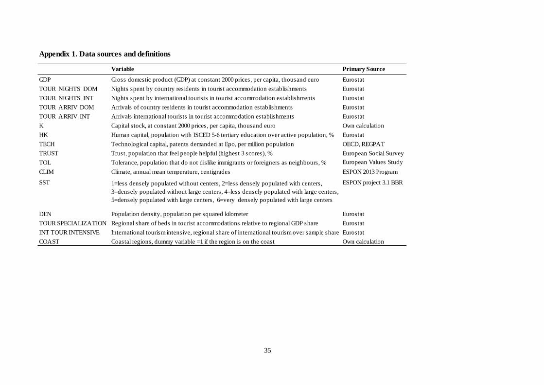
35

 

Appendix 1. Data sources and definitions

Variable Primary Source

GDP Gross domestic product (GDP) at constant 2000 prices, per capita, thousand euro Eurostat

TOUR NIGHTS DOM Nights spent by country residents in tourist accommodation establishments Eurostat

TOUR NIGHTS INT Nights spent by international tourists in tourist accommodation establishments Eurostat

TOUR ARRIV DOM Arrivals of country residents in tourist accommodation establishments Eurostat

TOUR ARRIV INT Arrivals international tourists in tourist accommodation establishments Eurostat

K Capital stock, at constant 2000 prices, per capita, thousand euro Own calculation

HK Human capital, population with ISCED 5-6 tertiary education over active population, % Eurostat

TECH Technological capital, patents demanded at Epo, per million population OECD, REGPAT

TRUST Trust, population that feel people helpful (highest 3 scores), % European Social Survey

TOL Tolerance, population that do not dislike immigrants or foreigners as neighbours, % European Values Study

CLIM Climate, annual mean temperature, centigrades ESPON 2013 Program

SST 1=less densely populated without centers, 2=less densely populated with centers, 3=densely populated without large centers, 4=less densely populated with large centers, 5=densely populated with large centers, 6=very densely populated with large centers

ESPON project 3.1 BBR

DEN Population density, population per squared kilometer Eurostat

TOUR SPECIALIZATION Regional share of beds in tourist accommodations relative to regional GDP share Eurostat

INT TOUR INTENSIVE International tourism intensive, regional share of international tourism over sample share Eurostat

COAST Coastal regions, dummy variable =1 if the region is on the coast Own calculation

Ultimi Contributi di Ricerca CRENoS I Paper sono disponibili in: Uhttp://www.crenos.itU

12/34 Fab io Cer ina , “Endogenous Growth and Susta inable Tour ism”

12/33 Miche l e Ba t t i s t i ,F i l i ppo Be l l o c , Mas s imo De l Gat t o , “Unbundl ing technology adopt ion and t fp a t the f i rm leve l . Do intang ib les mat ter?”

12/32 Mass imo De l Gat t o , F i l i ppo d i Mauro , J o s eph Grube r , Ben jamin Mande l , “The “Revea led” Compet i t iveness of U.S . Exports ”

12/31 Marin e l l a Cadon i , Robe r ta Me l i s , Al e s sandro Trudda , “Financ ia l Cr is i s : a new measure for r i sk of pens ion funds assets”

12/30 Oliv i e r o A. Carbon i , Pao l o Rus su , “Globa l Indeterminacy in a Tour ism Sector Model”

12/29 Oliv i e r o A. Carbon i , Pao l o Rus su , “A Model of Economic Growth wi th Publ ic F inance : Dynamics and Analy t ic So lut ion”

12/28 Maria Giovanna Brandano , C laud i o De to t t o , Mar co Vann in i , “Comparat ive ef f ic iency of producer cooperat ives and convent iona l f i rms in a sample of quas i - twin companies”

12/27 Bianca B iag i , Mar ia Giovanna Brandano , Diony s ia Lambi r i , “Does tour ism affect house pr ices? Some ev idence f rom Ita ly”

12/26 Gabr i e l e Cardu l l o , Maur iz i o Con t i , Giovann i Su l i s , “Sunk Capi ta l , Unions and the Hold-Up Problem: Theory and Evidence f rom Sectora l Data”

12/25 Fab io Cer ina , Fab i o Manca , “Catch me i f you learn : deve lopment-spec i f ic educat ion and economic growth”

12/24 Andrea Pozz i , Fab iano S ch i va rd i , “Demand or product iv i ty : What determines f i rm growth?”

12/23 Dimi t r i Pao l in i , Juan d e Dio s Tena , “Inst i tut iona l Complex i ty and Manager ia l Eff ic iency : A S imple Model”

12/22 Migue l Ja ra , Dimi t r i Pao l in i , Juan d e Dio s Tena , “Management Eff ic iency in Footba l l : An Empir ica l Ana lys i s of two Extreme Cases”

12/21 Marta Fodd i , S t e f ano Usa i , “Regiona l innovat ion performance in Europe”

12/20 Juan d e Dio s Tena , C laud i o De to t t o , Dimi t r i Pao l in i , “Do manager ia l sk i l l s mat ter? An ana lys i s of the impact of manager ia l fea tures on performance for the I ta l i an footba l l”

12/19 Claud io De to t t o , Bryan C. McCannon , Mar co Vann in i , “Unders tanding Ransom Kidnapping and I ts Durat ion”

12/18 Anna Mar ia P inna , “Vis i t and Buy . An Empir ica l Ana lys i s on Tour ism and Exports”

12/17 Edoardo Ot ran to , “Spi l lover Effects in the Vola t i l i ty of F inanc ia l Markets”

12/16 Manue la De idda , Adr iana Di Lib e r t o , Mar ta Fodd i , Giovann i Su l i s , “Employment Subs id ies , Informal Economy and Women’s Trans i t ion into Work in a Depressed Area : Evidence f rom a Matching Approach”

12/15 A. Debón , S . Habe rman , F . Mont e s , Edoardo Ot ran t o , “Model ef fect on pro jected morta l i ty ind icators”

www.crenos.it