workshop on approaches and applications of inductive
TRANSCRIPT

Workshop on Approaches and Applications of InductiveProgramming (AAIP)
to be held on August 7th 2005 in conjunction with the 22nd InternationalConference on Machine Learning (ICML 2005) in Bonn, Germany.
Organized by Emanuel Kitzelmann, Roland Olsson, Ute Schmid


Contents
Foreword 5
Program Committee 7
Invited Talks 8Stephen Muggleton:
Learning the Time Complexity of Logic Programs . . . . . . . . . . . . . 9Jurgen Schmidhuber:
How to Learn a Program: Optimal Universal Learners & Goedel Machines 11Fritz Wysotzki:
Development of Inductive Synthesis of Functional Programs . . . . . . . . 13
Full Papers 15Emanuel Kitzelmann, Ute Schmid:
An Explanation Based Generalization Approach to Inductive Synthesis ofFunctional Programs . . . . . . . . . . . . . . . . . . . . . . . . . . . . . . 15
Oleg Monakhov, Emilia Monakhova:Synthesis of Scientific Algorithms based on Evolutionary Computationand Templates . . . . . . . . . . . . . . . . . . . . . . . . . . . . . . . . . 29
A. Passerini, P. Frasconi, L. De Raedt:Kernels on Prolog Proof Trees: Statistical Learning in the ILP Setting . . 37
M. R. K. Krishna Rao:Learning Recursive Prolog Programs with Local Variables from Examples 51
Work in Progress 59Ramiro Aguilar, Luis Alonso, Vivian Lopez, Marıa N. Moreno:
Incremental discovery of sequential patterns for grammatical inference . . 59Palem GopalaKrishna:
Data-dependencies and Learning in Artificial Systems . . . . . . . . . . . 69
Author Index 81
3


Foreword
The ICML workshop AAIP 2005 – “Approaches and Applications of Inductive Program-ming” – was held at the 22nd International Conference on Machine Learning (ICML2005) in Bonn, Germany on 7th of August 2005. The main goal of AAIP was to bringtogether researchers from different areas of machine learning who are especially inter-ested in the inductive synthesis of programs from input/output examples.
Automatic induction of programs from input/output examples is an active area of re-search since the sixties and of interest for machine learning research as well as for auto-mated software engineering. In the early days of inductive programming research therewere proposed several approaches to the synthesis of Lisp programs from examples ortraces. Due to only limited progress, interest decreased in the mid-eighties and researchfocused on inductive logic programming (ILP) instead. Although ILP proved to be apowerful approach to learning relational concepts, applications to learning of recursiveclauses had only moderate success. Learning recursive programs from examples is alsoinvestigated in genetic programming and other forms of evolutionary computation. Hereagain, functional programs are learned from sets of positive examples together with anoutput evaluation function which specify the desired input/output behavior of the pro-gram to be learned. A fourth approach is learning recursive programs in the context ofgrammar inference.
Currently, there is no single prominent approach to inductive program synthesis. Instead,research is scattered over the different approaches. Nevertheless, inductive programmingis a research topic of crucial interest for machine learning and artificial intelligence ingeneral. The ability to generalize a program – containing control structures as recursionor loops – from examples is a challenging problem which calls for approaches goingbeyond the requirements of algorithms for concept learning. Pushing research forwardin this area can give important insights in the nature and complexity of learning as wellas enlarging the field of possible applications.
Typical areas of application where learning of programs or recursive rules are calledfor, are first in the domain of software engineering where structural learning, softwareassistants and software agents can help to relieve programmers from routine tasks, giveprogramming support for endusers, or support of novice programmers and programmingtutor systems. Further areas of application are language learning, learning recursivecontrol rules for AI-planning, learning recursive concepts in web-mining or for data-format transformations.
Today research on program induction is scattered over different communities. The AAIP2005 workshop brought together researchers from these different communities with thecommon interest on induction of general programs regarding theory, methodology andapplications. The three invited speakers represent inductive program synthesis researchin the areas of classical functional synthesis (Fritz Wysotzki, TU Berlin, Germany),inductive logic programming (Stephen Muggleton, Imperial College London, UK), and
5

optimal universal reinforcement learning (Jurgen Schmidhuber, IDSIA, Manno-Lugano,Switzerland). The four full papers and two work in progress reports are distributed overall areas mentioned above, that is, they address inductive functional synthesis, inductivelogic programming, evolutionary computation, and grammatical inference.
In our opinion, getting acquainted with other approaches to this problem, their rel-ative merits and limits, will strengthen research in inductive programming by cross-fertilization. We hope, that for the machine learning community at large the challengingtopic of program induction which is currently rather neglected, might come in the focusof interest.
We want to thank the all members of the program committee for their support in promot-ing the workshop and for reviewing submitted papers and we thank the ICML organizers,especially the workshop chair Hendrik Blockeel for technical support.
We are proud to present you the proceedings of the first workshop ever striving to coverall areas of program induction!
Emanuel Kitzelmann(Dept. of Information Systems and Applied Computer Science, Otto-Friedrich-University Bamberg, Germany)
Roland Olsson(Faculty of Computer Science, Østfold College, Norway)
Ute Schmid(Dept. of Information Systems and Applied Computer Science, Otto-Friedrich-University Bamberg, Germany)
6

Program Committee
Pierre FlenerComputing Science Division, Department of Information Technology, Uppsala Uni-versity, Sweden
Colin de la HigueraEURISE, Universite de Saint-Etienne, France
Emanuel Kitzelmann (co-organizer)Dept. of Information Systems and Applied Computer Science, Bamberg University,Germany
Steffen LangeDept. of Computer Science, University of Applied Sciences Darmstadt, Germany++49-6151-16-8441, [email protected]://www.fbi.fh-darmstadt.de/slange/
Stephen MuggletonComputational Bioinformatics Laboratory, Department of Computing, ImperialCollege,London, UK
Roland Olsson (co-organizer)Faculty of Computer Science, Østfold college, Halden, Norway
M.Jose RamırezDepartamento de Sistemas Informaticos y Computacion (DSIC), Universidad Politecnicade Valencia, Spain
Ute Schmid (co-organizer)Dept. of Information Systems and Applied Computer Science, Bamberg University,Germany
Fritz WysotzkiDept. of Electrical Engineering and Computer Science, Technical University Berlin,Germany
7


Learning the Time Complexity of LogicPrograms
Stephen Muggleton [email protected]
Computational Bioinformatics LaboratoryDepartment of ComputingImperial College, London, UK
One of the key difficulties in machine learning recursive logic programs is as-sociated with the testing of examples. Inefficient hypotheses, though usuallyof least interest to the learner, take more time to test. Almost by definition,efficient learners require a bias towards low-complexity hypotheses. However,it is unclear how such a bias can be implemented. To these ends, in this pre-sentation we address the problem of recognising inefficient logic programs. Tothe author’s knowledge, this problem has not been considered previously in theliterature. A successful approach to recognition of inefficient logic programsshould bring the prospects of effective machine learning of recursive logic pro-grams closer. In general the problem of recognising the time complexity ofan arbitrary program is incomputable since halting is undecidable. However,partial solutions cannot be ruled out. In this presentation we provide an ini-tial investigation of the problem based on developing a framework for machinelearning higher-order patterns associated with various complexity orders.
9


How to Learn a Program:Optimal Universal Learners & Goedel Machines
Jurgen Schmidhuber [email protected]
IDSIAManno-Lugano, Switzerland
Rational embedded agents should try to maximize future expected reward. Ingeneral, this requires learning an algorithm that uses internal states to remem-ber relevant past sensory inputs. Most machine learning algorithms, however,just learn reactive behaviors, where output depends only on the current input.Is there an optimal way of learning non-reactive behaviors in general, unknownenvironments? Our new insights affirm that the answer is yes. I will discussboth theoretical results on optimal universal reinforcement learning & GoedelMachines, and mention applications of the recent Optimal Ordered ProblemSolver.
Links related to this talk:
Cogbotlab:http://www.idsia.ch/~juergen/cogbotlab.html
Universal learning machines / Goedel Machines:http://www.idsia.ch/~juergen/unilearn.htmlhttp://www.idsia.ch/~juergen/goedelmachine.html
Optimal Ordered Problem Solver:http://www.idsia.ch/~juergen/oops.html
11


Development of Inductive Synthesis ofFunctional Programs
Fritz Wysotzki [email protected]
Technische Universitat Berlin
Inductive program synthesis is yet in the state of fundamental research. Thetask consists of inductive construction of a program from pairs of given input-output examples or instantiated initial parts of the intended program usingspecific methods of generalisation. Well known is the field of Inductive LogicProgramming (ILP) which is concerned with the induction of logical programs.The pioneering work in synthesis of functional programs was done by Summers1977 using the programming language LISP. Summers approach was restrictedto structural list problems i.e. his algorithms depend on the structure of a listbut not of its content. After Summers other work on synthesis of functionalprograms was done using LISP, too. The main topic of this lecture will be thesynthesis of functional programs in an abstract formalism, i.e. without using aspecial programming language. The basis are mainly theoretical investigationsand programmed realisations of the algorithms which have been performedat the TU Berlin over many years. The lecture starts with some historicalremarks, after that the theoretical basis is introduced. It is a term algebraincluding a special non-strict term (corresponding to the IF-THEN-ELSE) forrealizing tests. A functional program is represented by a system of equationsthe left hand side of which are function variables (Onames of subprogramsO)with parameters (Oformal parametersO), the right hand sides are terms, whichmay contain the function variables and there is a special term representingthe Omain programO. This system is called Recursive Program Scheme (RPS,Courcelle and Nivat 1978). It can be OsolvedO syntactically by an orderedsequence of finite terms (KLEENE-sequence), approximating the fixpoint so-lution which is an infinite term. This corresponds to unfolding the RPS.Theinduction principle works as follows: If one has a finite example term (i.e. withinstantiated variables) one can try to Oexplain itO as being an element of aKLEENE-sequence of an RPS. Extrapolation with introduction of variables asgeneralisation principle and folding gives a hypothetical RPS which explainsthe given example term. The reliability of the hypothesis depends on the po-sition of the given term in the KLEENE-sequence. One of the main problemswhich will be discussed is the detection and induction of subprograms in theexample term by finding an appropriate segmentation. Another problem is howto get the example term. Two domain dependent approaches will be discussed:the integration of (mutually excluding) production rules and planning. In thelatter case from a problem solving graph a shortest path tree (Universal Plan)is constructed. In the second step by a generalisation procedure similar tosubsumption used in ILP a goal hierarchy is computed. This goal tree is thentransformed into an initial program (program tree) which can be used as a ba-sis for inductive construction of a RPS mentioned above. The main principlesof our approach to the inductive construction of functional programs will bedemonstrated by examples.
13


An Explanation Based Generalization Approach to Inductive Synthesis ofFunctional Programs
Emanuel Kitzelmann [email protected]
Ute Schmid [email protected]
Department of Information Systems and Applied Computer Science, Otto-Friedrich-University, Bamberg
AbstractWe describe an approach to the inductive syn-thesis of recursive equations from input/output-examples which is based on the classical two-step approach to induction of functional Lispprograms of Summers (1977). In a first step, I/O-examples are rewritten to traces which explainthe outputs given the respective inputs based ona datatype theory. This traces can be integratedinto one conditional expression which representsa non-recursive program. In a second step, thisinitial program term is generalized into recursiveequations by searching for syntactical regulari-ties in the term. Our approach extends the classi-cal work in several aspects. The most importantextensions are that we are able to induce a set ofrecursive equations in one synthesizing step, theequations may contain more than one recursivecall, and additionally needed parameters are au-tomatically introduced.
1. Introduction
Automatic induction of recursive programs frominput/output-examples (I/O-examples) is an active area ofresearch since the sixties and of interest for AI researchas well as for software engineering (Lowry & McCarthy,1991; Flener & Partridge, 2001). In the seventies andeighties, there were several approaches to the synthesisof Lisp programs from examples or traces (see Biermannet al., 1984 for an overview). The most influential approachwas developed by Summers (1977), who put inductivesynthesis on a firm theoretical foundation.
Summers’ early approach is an explanation based gener-alization (EBG) approach, thus it widely relies on algo-rithmic processes and only partially on search: In a firststep, traces—steps of computations executed from a pro-gram to yield an output from a particular input—and predi-cates for distinguishing the inputs are calculated for eachI/O-pair. Construction of traces, which are terms in the
classical functional approaches, relies on knowledge of theinductive datatype of the inputs and outputs. That is, tracesexplain the outputs based on a theory of the used datatypegiven the respective inputs. The classical approaches forsynthesizing Lisp-programs used the general Lisp datatypeS-expression. By integrating traces and predicates into aconditional expression a non-recursive program explainingall I/O-examples is constructed as result of the first syn-thesis step. In a second step, regularities are searched forbetween the traces and predicates respectively. Found reg-ularities are then inductively generalized and expressed inform of the resulting recursive program.
The programs synthesized by Summers’ system contain ex-actly one recursive function, possibly along with one con-stant term calling the recursive function. Furthermore, allsynthesizable functions make use of a small fixed set ofLisp-primitives, particularly of exactly one predicate func-tion, atom, which tests whether its argument is an atom,e.g., the empty list. The latter implies two things: First,that Summers’ system is restricted to induce programs forstructural problems on S-expressions. That means, that ex-ecution of induced programs depends only on the structureof the input S-expression, but never on the semantics of theatoms contained in it. E.g., reversing a list is a structuralproblem, yet not sorting a list. The second implication is,that calculation of the traces is a deterministic and algorith-mic process, i.e. does not rely on search and heuristics.
Due to only limited progress regarding the class of pro-grams which could be inferred by functional synthesis,interest decreased in the mid-eighties. There was a re-newed interest of inductive program synthesis in the fieldof inductive logic programming (ILP) (Flener & Yilmaz,1999; Muggleton & De Raedt, 1994), in genetic program-ming and other forms of evolutionary computation (Olsson,1995) which rely heavily on search.
We here present an EBG approach which is based on themethodologies proposed by Summers (1977). We regardthe functional two-step approach as worthwhile for the fol-lowing reasons: First, algebraic datatypes provide guid-
15

An Explanation Based Generalization Approach to Inductive Synthesis of Functional Programs
ance in expressing the outputs in terms of the inputs as firstsynthesis step. Second, it enables a seperate and therebyspecialized handling of a knowledge dependent part and apurely syntactic driven part of program synthesis. Third,both using algebraic datatypes and seperating a knowledge-dependent from a syntactic driven part enables a more ac-curate utilization of search than in ILP or evolutionary pro-gramming. Fourth, the two-step approach using algebraicdatatypes provides a systematic way to introduce auxiliaryrecursive equations if necessary.
Our approach extends Summers in several important as-pects, such that we overcome fundamental restrictions ofthe classical approaches to induction of Lisp programs:First, we are able to induce a set of recursive equations inone synthesizing step, second, the equations may containmore than one recursive call, and third, additionally neededparameters are automatically introduced. Furthermore, ourgeneralization step is domain-independent, in particular in-dependent from a certain programming language. It takesas input a first-order term over an arbitrary signature andgeneralizes it to a recursive program scheme, that is, a setof recursive equations over that signature. Hence it canbe used as learning component in all domains which canrepresent their objects as recursive program schemes andprovide a system for solving the first synthesis step. E.g.,we use the generalization algorithm for learning recursivecontrol rules for AI planning problems (cp. Schmid &Wysotzki, 2000; Wysotzki & Schmid, 2001).
2. Central Concepts and an Example
The three central objects dealt with by our system are(1) sets of I/O-examples specifying the algorithm to beinduced, (2) initial (program) terms explaining the I/O-examples, and (3) recursive program schemes (RPSs) rep-resenting the induced algorithms. Their functional role inour two-step synthesis approach is shown in Fig. 1.
An example for I/O-examples is given in Tab. 1. The exam-ples specify the lasts function which takes a list of lists asinput and yields a list of the last elements of the lists as out-put. In the first synthesis step, an initial term is constructedfrom these examples. An initial term is a term respecting anarbitrary first-order signature extended by the special con-stant symbol Ω, meaning the undefined value and directinggeneralization in the second synthesis step. Suitably in-terpreted, an initial term evaluates to the specified outputwhen its variable is instantiated with a particular input ofthe example set and to undefined for all other inputs.
Tab. 2 gives an example of an initial term. It shows the re-sult of applying the first synthesis step to the I/O-examplesfor the lasts function as shown in Tab. 1. if means the 3arynon-strict function which returns the value of its second pa-
Table 1. I/O-examples for lasts
[] 7→ [],[[a]] 7→ [a],
[[a,b]] 7→ [b],[[a,b,c]] 7→ [c],
[[a,b,c,d]] 7→ [d],[[a], [b]] 7→ [a,b],
[[a], [b,c]] 7→ [a,c],[[a,b], [c], [d]] 7→ [b,c,d],
[[a,b], [c,d], [e, f ]] 7→ [b,d, f ],[[a], [b], [c], [d]] 7→ [a,b,c,d]
rameter if its first parameter evaluates to true and otherwisereturns the value of its third parameter; empty is a predicatewhich tests, whether its argument is the empty list; hd andtl yield the first element and the rest of a list respectively;cons constructs a list from one element and a list; and []denotes the empty list.
Table 2. Initial term for lastsif(empty(x), [],cons(hd(if(empty(tl(hd(x))), hd(x),if(empty(tl(tl(hd(x)))), tl(hd(x)),if(empty(tl(tl(tl(hd(x))))), tl(tl(hd(x))),
Ω)))) ,if(empty(tl(x)), [],cons(hd(if(empty(tl(hd(tl(x)))), hd(tl(x)),
Ω)) ,if(empty(tl(tl(x))), [],cons(hd(if(empty(tl(hd(tl(tl(x))))), hd(tl(tl(x))),
Ω)) ,if(empty(tl(tl(tl(x)))), [],
Ω)))))))
Calculation of initial terms relies on knowledge of thedatatypes of the example inputs and outputs. For our exem-plary lasts program inputs and outputs are lists. Lists areuniquely constructed by means of the empty list [] and theconstructor cons. Furthermore they are uniquely decom-posed by the functions hd and tl. That allows to calculatea unique term which expresses an example output in termsof the input. For example, consider the third I/O-examplefrom Tab. 1: If x denotes the input [[a,b]], then the termcons(hd(tl(hd(x))), []) expresses the specified output [b] interms of the input. Such traces are constructed for eachI/O-pair. The overall concept for integrating the resultingtraces into one initial term is to go through all traces in par-allel position by position. If the same function symbol iscontained at the current position in all traces, then it is in-
16

An Explanation Based Generalization Approach to Inductive Synthesis of Functional Programs
I/O-examples
1. Step: Explanation,
based on knowledge of datatypes−−−−−−−−−−−−−−−−−−−→ Initial Term
2. Step: Generalization,
purely syntactic driven−−−−−−−−−−−−−−−→ Recursive Program Scheme
Figure 1. Two synthesis steps
troduced to the initial term at this position. If at least twotraces differ at the current position, then it is introduced anif -expression. Therefore a predicate function is calculatedto discriminate the inputs according to the different traces.Construction of the initial term proceeds from the discrim-inated inputs and traces for the second and third branch ofthe if -tree respectively. We describe the calculation of ini-tial terms from I/O-examples, i.e. the first synthesis step,in Sec. 4.
In the second synthesis step, initial ground terms are gener-alized to a recursive program scheme. Initial terms are con-sidered as (incomplete) unfoldings of an RPS which is to beinduced by generalization. An RPS is a set of recursiveequations whose left-hand-sides consist of the names ofthe equations followed by their parameter lists and whoseright-hand-sides consist of terms over the signature fromthe initial terms, the set of the equation names, and the pa-rameters of the equations. One equation is distinguishedto be the main one. An example is given in Tab. 3. ThisRPS, suitably interpreted, computes the lasts function asdescribed above and specified by the examples in Tab. 1. It
Table 3. Recursive Program Scheme for lasts
lasts(x) = if(empty(x), [],
cons(hd(last(hd(x))), lasts(tl(x))))
last(x) = if(empty(tl(x)),x, last(tl(x)))
results from applying the second synthesis step to the ini-tial term shown in Tab. 2. Note that it is a generalizationfrom the initial term in that it not merely computes the lastsfunction for the example inputs but for input-lists of arbi-trary length containing lists of arbitrary length.
The second synthesis step does not depend on domainknowledge. The meaning of the function symbols is irrel-evant, because the generalization is completely driven bydetecting syntactical regularities in the initial terms. Tounderstand the link between initial terms and RPSs in-duced from them, we consider the process of incremen-tally unfolding an RPS. Unfolding of an RPS is a (non-deterministic and possibly infinite) rewriting process whichstarts with the instantiated head of the main equation of anRPS and which repeatedly rewrites a term by substitutingany instantiated head of an equation in the term with ei-ther the equally instantiated body or with the special sym-
bol Ω. Unfolding stops, when all heads of recursive equa-tions in the term are rewritten to Ω, i.e., the term containsno rewritable head any more. Consider the last equationfrom the RPS shown in Tab. 3 and the initial instantia-tion x 7→ [a,b,c]. We start with the instantiated headlast([a,b,c]) and rewrite it to the term:
if(empty(tl([a,b,c])), [a,b,c], last(tl([a,b,c])))
This term contains the head of the last equation instantiatedwith x 7→ tl([a,b,c]). When we rewrite this head againwith the equally instantiated body we obtain:
if(empty(tl([a,b,c])), [a,b,c],
if(empty(tl(tl([a,b,c]))), tl([a,b,c]),
last(tl(tl([a,b,c]))))
This term now contains the head of the equation instanti-ated with x 7→ tl(tl([a,b,c])). We rewrite it once againwith the instantiated body and then replace the head in theresulting term with Ω and obtain:
if(empty(tl([a,b,c])), [a,b,c],
if(empty(tl(tl([a,b,c]))), tl([a,b,c]),
if(empty(tl(tl(tl([a,b,c])))), tl(tl([a,b,c])),Ω)))
The resulting finite term of a finite unfolding process is alsocalled unfolding. Unfoldings of RPSs contain regularitiesif the heads of the recursive equations are more than oncerewritten with its bodies before they are rewritten with Ωs.The second synthesis step is based on detecting such regu-larities in the initial terms.
We describe the generalization of initial terms to RPSs inthe following section. The reason why we first describe thesecond synthesis step and only afterwards the first synthesisstep is, that the latter is governed by the goal of construct-ing a term which can be generalized in the second step.Therefore, for understanding the first step, it is necessaryto know the connection between initial terms and RPSs asestablished in the second step.
3. Generalizing an Initial Term to an RPS
Since our generalization algorithm exploits the relation be-tween an RPS and its unfoldings, in the following we willfirst introduce the basic terminology for terms, substitu-tions, and term rewriting as for example presented in Der-showitz and Jouanaud (1990). Then we will present defi-nitions for RPSs and the relation between RPSs and their
17

An Explanation Based Generalization Approach to Inductive Synthesis of Functional Programs
unfoldings. The set of all possible RPSs constitutes thehypothesis language for our induction algorithm. Somerestrictions on this general hypothesis language are intro-duced and finally, the componentes of the generalizationalgorithm are described.
3.1. Preliminaries
We denote the set of natural numbers starting with 0 by N
and the natural numbers greater 0 by N+. A signature Σis a set of (function) symbols with α : Σ→ N giving thearity of a symbol. We write TΣ for the set of ground terms,i.e. terms without variables, over Σ and TΣ(X) for the setof terms over Σ and a set of variables X . We write TΣ,Ωfor the set of ground terms—called partial ground terms—constructed over Σ∪ Ω, where Ω is a special constantsymbol denoting the undefined value. Furthermore, wewrite TΣ,Ω(X) for the set of partial terms constructed overΣ∪Ω and variables X . With T ∞
Σ,Ω(X) we denote the set ofinifinite partial terms over Σ and variables X . Over the setsTΣ,Ω, TΣ,Ω(X) and T ∞
Σ,Ω(X) a complete partial order (CPO)≤ is defined by: a) Ω≤ t for all t ∈ TΣ,Ω,TΣ,Ω(X),T ∞
Σ,Ω(X)
and b) f (t1, . . . , tn)≤ f (t ′1, . . . , t′n) iff ti ≤ t ′i for all i ∈ [1;n].
Terms can uniquely be expressed as labeled trees: If a termis a constant symbol or a variable, then the correspondingtree consists of only one node labeled by the constant sym-bol or variable. If a term has the form f (t1, . . . , tn), thenthe root node of the corresponding tree is labeled with fand contains from left to right the subtrees correspondingto t1, . . . , tn. We use the terms tree and term as synonyms.A position of a term/tree is a sequence of positive naturalnumbers, i.e. an element from N
∗+ . The set of positions
of a term t, denoted pos(t), contains the empty sequence εand the position iu, if the term has the form t = f (t1, . . . , tn)and u is a position from pos(ti), i ∈ [1;n]. Each positionof a term uniquely denotes one subterm. We write t|u fordenoting that subterm which is determined as follows: (a)t|ε = t, (b) if t = f (t1, . . . , tn) and u is a position in ti, thent|iu = ti|u, i ∈ [1;n]. We say that position u is smaller thanposition u′, u ≤ u′, if u is a prefix of u′. If u is a positionof term t and u′ ≤ u, then u′ is a position of t. For a term tand a position u, node(t,u) denotes the fixed symbol f ∈ Σ,if t|u = f (t1, . . . , tn) or t|u = f respectively. The set of allpositions at which a fixed symbol f appears in a term is de-noted by pos(t, f ). The replacement of a subterm t|u by aterm s in a term t at position u is written as t[u← s]. Let Udenote a set of positions in a term t. Then t[U← s] denotesthe replacement of all subterms t|u with u ∈U by s in t.
A substitution σ is a mapping from variables to terms. Sub-stitutions are naturally continued to mappings from termsto terms by σ( f (t1, . . . , tn)) = f (σ(t1), . . . ,σ(tn)). Substi-tutions are written in postfix notation, i.e. we write tσ in-stead of σ(t). Substitutions β : X → TΣ from variables to
ground terms are called (variable) instantiations. A term pis called pattern of a term t, iff t = pσ for a substitution σ .A pattern p of a term t is called trivial, iff p is a variableand non-trivial otherwise. We write t ≤s p iff p is a patternof t and t <s p iff additionally holds, that p and t can notbe unified by variable renaming only.
A term rewriting system (TRS) over Σ and X is a set ofpairs of terms R ⊆ TΣ(X)×TΣ(X). The elements (l,r) ofR are called rewrite rules and are written l→ r. A term t ′
can be derived in one rewrite step from a term t using R
(t→R t ′), if there exists a position u in t, a rule l→ r ∈R,and a substitution σ : X → TΣ(X), such that (a) t|u = lσand (b) t ′ = t[u← rσ ]. R implies a rewrite relation→R⊆TΣ(X)×TΣ(X) with (t, t ′) ∈→R if t→R t ′.
3.2. Recursive Program Schemes
Definition 1 (Recursive Program Scheme). Given a sig-nature Σ, a set of function variables Φ = G1, . . . ,Gn fora natural number n > 0 with Σ∩Φ = /0 and arity α(Gi) > 0for all i ∈ [1;n], a natural number m ∈ [1;n], and a set ofequations
G =
G1(x1, . . . ,xα(G1)) = t1,
...
Gn(x1, . . . ,xα(Gn)) = tn
where the ti are terms with respect to the signature Σ∪Φand the variables x1, . . . ,xα(Gi), S = (G ,m) is an RPS.Gm(x1, . . . ,xα(Gm)) = tm is called the main equation of S .
The function variables in Φ are called names of the equa-tions, the left-hand-sides are called heads, the right-hand-sides bodies of the equations. For the lasts RPS shown inTab. 3 holds: Σ = if ,empty,cons,hd, tl, [], Φ = G1,G2with G1 = lasts and G2 = last, and m = 1. G is the set ofthe two equations.
We can identify a TRS with an RPS S = (G ,m):
Definition 2 (TRS implied by an RPS). Let be S =(G ,m) an RPS over Σ, Φ and X , and Ω the bottom sym-bol in TΣ,Ω(X). The equations in G constitute rules RS =Gi(x1, . . . ,xα(Gi)) → ti | i ∈ [1;n] of a term rewritingsystem. The system additionally contains rules RΩ =Gi(x1, . . . ,xα(Gi))→Ω | i ∈ [1;n], Gi is recursive.
The standard interpretation of an RPS, called free interpre-tation, is defined as the supremum in T ∞
Σ,Ω(X) of the setof all terms in TΣ,Ω(X) which can be derived by the im-plied TRS from the head of the main equation. Two RPSsare called equivalent, iff they have the same free interpre-tation, i.e. if they compute the same function for every in-terpretation of the symbols in Σ. Terms in TΣ,Ω which canbe derived by the instantiated head of the main equation
18

An Explanation Based Generalization Approach to Inductive Synthesis of Functional Programs
regarding some instantiation β : X → TΣ are called unfold-ings of an RPS relative to β . Note, that terms derived fromRPSs are partial and do not contain function variables, i.e.all heads of the equations are eventually rewritten by Ωs.
The goal of the generalization step is to find an RPS whichexplains a set of initial terms, i.e. to find an RPS such thatthe initial terms are unfoldings of that RPS. We denote ini-tial terms by t and a set of initial terms by I . We liberalizeI such that it may include incomplete unfoldings. Incom-plete unfoldings are unfoldings, where some subtrees con-taining Ωs are replaced by Ωs.
We need to define four further concepts, namely recursionpositions which are positions in the equation bodies whererecursive calls appear, substitution terms which are the ar-gument terms in recursive calls, unfolding positions whichare positions in unfoldings at which the heads of the equa-tions are rewritten with their bodies, and finally parameterinstantiations in unfoldings which are subterms of unfold-ings resulting from the initial parameter instantiation andthe substitution terms:
Definition 3 (Recursion Positions and SubstitutionTerms). Let G(x1, . . . ,xα(G)) = t with parameters X =x1, . . . ,xα(G) be a recursive equation. The set of recur-sion positions of G is given by R = pos(t,G). Each recur-sive call of G at position r ∈ R in t implies substitutionsσr : X → TΣ(X) : x j 7→ t|r j for all j ∈ [1;α(G)] for the pa-rameters in X . We call the terms t|r j substitution terms ofG.
For equation lasts of the lasts RPS (Tab. 3) holds R = 32and xσ 32 = tl(x). For equation last holds R = 3 andxσ 3 = tl(x).
Now consider an unfolding process of a recursive equationand the positions at which rewrite steps are applied in theintermediate terms. The first rewriting is applied at root-position ε , since we start with the instantiated head of theequation which is completely rewritten with the instanti-ated body. In the instantiated body, rewrites occur at recur-sion positions R. Assume that on recursion position r ∈ Rthe instance of the head is rewritten with an instance of thebody. Then, relative to the resulting subtree at position r,rewrites occur again at recursion positions, e.g. at positionr′ ∈ R. Relative to the entire term these latter rewrites occurtherefore at compositions of position r and recursion posi-tions, e.g. at position rr′ and so on. We call the infinite setof positions at which rewrites can occur in the intermediateterms within an unfolding of a recursive equation unfoldingpositions. They are determined by the recursion positionsas follows:
Definition 4 (Unfolding Positions). Let be R the recursionpositions of a recursive equation G. The set of unfoldingpositions U of G is defined as the smallest set of positions
which contains the position ε and, if u ∈U and r ∈ R, theposition ur.
The unfolding positions of equation lasts of the lasts RPSare 32,3232,323232, . . ..
Now we look at the variable instantiations occuring duringunfolding a recursive equation. Recall the unfolding pro-cess of the last equation (see Tab. 3) described at the endof Sec. 2. The initial instantiation was βε = β = x 7→[a,b,c], thus in the body of the equation (replaced for theinstantiated head as result of the first rewrite step), its vari-able is instantiated with this initial instantiation. Due tothe substitution term tl(x), the variable of the head in thisbody is instantiated with β3 = σ 3 βε = x 7→ tl([a,b,c]),i.e. the variable in the body replaced for this instantiatedhead is instantiated with σ 3 βε . A further rewriting stepimplies the instantiation β33 = σ 3 σ 3 βε = σ 3 β3 = x 7→tl(tl([a,b,c])) and so on. We index the instantiations oc-curing during unfolding with the unfolding positions atwhich the particular instantiated heads were placed. Theyare determined by the substitutions implied by recursivecalls and an initial instantiation as follows:
Definition 5 (Instantiations in Unfoldings). Let beG(x1, . . . ,xα(G)) = t a recursive equation with parametersX = x1, . . . ,xα(G), R and U the recursion positions andunfolding positions of G resp., σ r the substitutions impliedby the recursive call of G at position r ∈ R, and β : X → TΣan initial instantiation. Then a family of instantiations in-dexed over U is defined as βε = β and βur = σ r βu foru ∈U,r ∈ R.
3.3. Restrictions and the Generalization Problem
An RPS which can be induced from initial terms is re-stricted in the following way: First, it contains no mu-tual recursive equations, second, there are no calls of re-cursive equations within calls of recursive equations (nonested recursive calls). The first restriction is not a seman-tical restriction, since each mutual recursive program canbe transformed to an equivalent (regarding a particular al-gebra) non-mutual recursive program. Yet it is a syntac-tical restriction, since unfoldings of mutual RPSs can notbe generalized using our approach. A restriction similar tothe second one was stated by Rao (2004). He names TRSscomplying with such a restriction flat TRSs.
Inferred RPSs conform to the following syntactical charac-teristics: First, all equations, potentially except of the mainequation, are recursive. The main equation may be recur-sive as well, but, as only equation, it is not required to be re-cursive. Second, inferred RPSs are minimal, in that (i) eachequation is directly or indirectly (by means of other equa-tions) called from the main equation, and (ii) no parameterof any equation can be omitted without changing the free
19

An Explanation Based Generalization Approach to Inductive Synthesis of Functional Programs
interpretation. RPSs complying with the stated restrictionsand characteristics are called minimal, non-mutual, flat re-cursive program schemes.
There might be several RPSs which explain an initial termt, but have different free interpretations. For example, Ω isan unfolding of every RPS with a recursive main equation.Therefore, an important question is which RPS will be in-duced. Summers (1977) required that recurrence relationshold at least over three succeeding traces and predicatesto justify a generalization. A similar requirement wouldbe that induced RPSs explain the initial terms recurrently,meaning that I contains at least one term t which can bederived from an unfolding process, in which each recursiveequation had to be rewritten at least three times with itsbody. We use a slightly different requirement: One char-acteristic of minimal RPSs is, that if at least one substitu-tion term is replaced by another, then the resulting RPS hasa different free interpretation. We call this characteristicsubstitution uniqueness. Thus, it is sensible to require thatinduced RPSs are substitution unique regarding the initialterms, i.e. that if some substitution term is changed, thenthe resulting RPS no longer explains the initial terms. Itholds, that a minimal RPS explains a set of initial trees re-currently, if it explains it substitution uniquely.
Thus the problem of generalizing a set of initial terms I
to an RPS is to find an RPS which explains I and whichis substitution unique regarding I .
3.4. Solving the Generalization Problem
We will not state the generalization algorithm in detailin this section but we will describe the underlying con-cepts and the algorithm in a more informal manner. Forthis section and its subsections we use the term body ofan equation for terms which are strictly speaking incom-plete bodies: They contain only the name of the equationinstead of complete recursive calls including substitutionterms at recursion positions. For example, we refer tothe term if (empty(x), [],cons(hd(last(hd(x))), lasts)) as thebody for equation lasts of the lasts RPS (see Tab. 3). Thereason is, that we infer the complete body in two steps:First the term which we name body in this context, secondthe substitution terms for the recursive calls.
Generalization of a set of initial terms to an RPS is done inthree successive steps, namely segmentation of the terms,construction of equation bodies and calculation of substi-tution terms. These three generalization steps are orga-nized in a divide-and-conquer algorithm, where backtrack-ing can occur to the divide-phase. Segmentation consti-tutes the divide-phase which proceeds top-down throughthe initial terms. Within this phase recursion positions (seeDef. 3) and positions indicating further recursive equationsare searched for each induced equation. The latter set of
positions is called subscheme positions (see Def. 6 below).Found recursion positions imply unfolding positions (seeDef. 4). As result of the divide-phase the initial terms aredivided into several parts by the subscheme positions, suchthat—roughly speaking—each particular part is assumed tobe an unfolding of one recursive equation. Furthermore, theparticular parts are segmented by the unfolding positions,such that—roughly speaking—each segment is assumed tobe the result of one unfolding step of the respective recur-sive equation.
Consider the initial tree in Fig. 2, it represents the initialterm for lasts, shown in Tab. 2. The curved lines on thepath to the rightmost Ω divide the tree into three segmentswhich correspond to unfolding steps of the main equation,i.e. equation lasts. The short broad lines denote three sub-trees which are—except of their root hd—unfoldings of thelast equation. The curved lines within these subtrees divideeach subtree into segments, such that each segment corre-spond to one unfolding step of the last equation.
When the initial trees are segmented, calculation ofequation bodies and of substitution terms follows withinthe conquer-phase. These two steps proceed bottom-upthrough the divided initial trees and reduce the trees dur-ing this process. The effect is, that bodies and substitutionterms for each equation are calculated from trees whichare unfoldings of only the currently induced equation andhence, each segment in these trees is an instantiation of thebody of the currently induced equation. E.g., for the laststree shown in Fig. 2, a body and substitution terms are firstcalculated from the three subtrees, i.e. for the last equa-tion. Since there are no further recursive equations calledby the last equation—i.e. the segments of the three sub-trees contain themselves no subtrees which are unfoldingsof further equations—each segment is an instantiation ofthe body of the last equation. When this equation is com-pletely inferred, the three subtrees are replaced by suitableinstantiations of the head of the inferred last equation. Theresulting reduced tree is an unfolding of merely one recur-sive equation, the lasts equation. The three segments inthis reduced tree—indicated by the curved lines on the pathto the rightmost Ω—are instantiations of the body of thesearched for lasts equation. From this reduced tree, bodyand substitution terms for the lasts equation are inducedand the RPS is completely induced.
Segmentations are searched for, whereas calculation ofbodies and substitution terms are algorithmic. Constructionof bodies always succeeds, whereas calculation of substitu-tion terms—such that the inferred RPS explains the initialterms—may fail. Thus, an inferred RPS can be seen as theresult of a search through a hypothesis space where the hy-potheses are segmentations (divide-phase), and a construc-tive goal test, including construction of bodies and calcu-
20

An Explanation Based Generalization Approach to Inductive Synthesis of Functional Programs
hd
x
tl
tl
tl
x
tl
x
tl
hd
x
tl
hd
x
tl
x
hd
x
tl
x
hd
x
tl
x
tl
[]
[]empty
tl
x
hd
tl
empty
tl
empty
x
tl
tl
tl tl
empty
tl
hd
x
[]empty
[]empty
empty
x
empty
tl
hd
tl
empty
tl
hd
tl
hd
tl
cons
hd
if
if
Omega
Omega
if
if
cons
if
cons
if
if
Omega
hd
if
Omega
hd
if
Figure 2. Initial Tree for lasts
lation of substitution terms (conquer-phase), which tests,whether the completely inferred RPS explains the initialterms (and is substitution unique regarding them). In thefollowing we describe each step in more detail:
3.4.1. SEGMENTATION
When induction of an RPS from a set of initial trees I
starts, the hypothesis is, that there exists an RPS with a re-cursive main equation which explains I . First, recursionand subscheme positions for the hypothetical main equa-tion Gm are searched for.
Definition 6 (Subscheme Positions). Subscheme posi-tions are all smallest positions in the body of a recursiveequation G which denote subterms, in which calls of fur-ther recursive equations from the RPS appear, but no re-cursive call of equation G.
E.g., the only subscheme position of equation lasts of thelasts RPS (Tab. 3) is u = 31. A priori, only particular posi-tions from the initial trees come into question as recursionand subscheme positions, namely those which belong to apath leading from the root to an Ω. The reason is, thateventually each head of a recursive equation at any unfold-ing position in an intermediate term while unfolding thisequation is rewritten with an Ω:
Lemma 1 (Recursion and Subscheme Positions implyΩs). Let t ∈ TΣ,Ω be an (incomplete) unfolding of an RPSS = (G ,m) with a recursive main equation Gm. Let R, Uand S be the sets of recursion, unfolding and subschemepositions of Gm respectively. Then for all u ∈ U ∩ pos(t)holds:
1. pos(t|u,Ω) 6= /0
2. ∀s ∈ S : if us ∈ pos(t) then pos(t|us,Ω) 6= /0
It is not very difficult to see that this lemma holds. Fora lack of space we do not give the proof here. It can befound in (Kitzelmann, 2003) where Lem. 1 and Lem. 2 areproven as one lemma. Knowing Lem. 1, before searchstarts, the initial trees can be reduced to their skeletonswhich are terms resulting from replacing subtrees withoutΩs with variables.
Definition 7 (Skeleton). The skeleton of a term t ∈TΣ,Ω(X), written skeleton(t) is the minimal pattern of t forwhich holds pos(t,Ω) = pos(skeleton(t),Ω).
For example, consider the subtree indicated by the leftmostshort broad line of the tree in Fig. 2. Omitting the roothd, it is an unfolding of the last equation of the lasts RPSshown in Tab. 3. Its skeleton is the substantially reducedterm if (x1,x2, if (x3,x4, if (x5,x6,Ω))). Search for recursionand subscheme positions is done on the skeletons of theoriginal initial trees. Thereby the hypothesis space is sub-stantially narrowed without restricting the hypothesis lan-guage, since only those hypotheses are ruled out which area priori known to fail the goal test.
Ωs are not only implied by recursion and subscheme posi-tions, but also imply Ωs recursion and subscheme positionssince Ωs in unfoldings result only from rewriting an instan-tiated head of a recursive equation in a term with an Ω:
Lemma 2 (Ωs imply recursion and subscheme posi-tions). Let t ∈ TΣ,Ω be an (incomplete) unfolding of an RPSS = (G ,m) with a recursive main equation Gm. Let R, U
21

An Explanation Based Generalization Approach to Inductive Synthesis of Functional Programs
and S be the sets of recursion, unfolding and subscheme po-sitions of Gm respectively. Then for all v ∈ pos(t,Ω) hold
• It exists an u ∈U ∩pos(t),r ∈ R with u≤ v < ur or
• it exists an u ∈U ∩pos(t),s ∈ S with us≤ v.
Proof: in (Kitzelmann, 2003).
From the definition of subscheme positions and the pre-vious lemma follows, that subscheme positions are deter-mined, if a set of recursion positions has been fixed. Lem. 1restricts the set of positions which come into question asrecursion and subscheme positions. Lem. 2 together withcharacteristics from subscheme positions suggests to or-ganize the search as a search for recursion positions witha depending parallel calculation of subscheme positions.When hypothetical recursion, unfolding, and subschemepositions are determined they are checked regarding the la-bels in the initial trees on pathes leading to Ωs. The nodesbetween one unfolding position and its successors in un-foldings result from the same body (with different instanti-ations). Since variable instantiations only occur in subtreesat positions not belonging to pathes leading to Ωs, for eachunfolding position the nodes between it and its successorsare necessarily equal:
Lemma 3 (Valid Segmentation). Let t ∈ TΣ,Ω be an un-folding of an RPS S = (G ,m) with a recursive mainequation Gm. Then it exists a term tG ∈ TΣ,Ω(X) withpos(tG,Ω) = R∪ S such that for all u ∈ U ∩ pos(t) hold:tG ≤Ω t|u where ≤Ω is defined as (a) Ω≤Ω t if pos(t,Ω) 6=/0, (b) x ≤Ω t if x ∈ X and pos(t,Ω) = /0, and (c)f (t1, . . . , tn)≤Ω f (t ′1, . . . , t
′n) if ti ≤Ω t ′i for all i ∈ [1;n].
Proof: in (Kitzelmann, 2003).
This lemma has to be slightly extended, if one allows forinitial trees which are incomplete unfoldings. Lem. 3 statesthe requirements to assumed recursion and subscheme po-sitions which can be assured at segmentation time. Theyare necessary for an RPS which explains the initial terms,yet not sufficient to assure, that an RPS complying withthem exists which explains the initial trees. That is, later abacktrack can occur to search for other sets of recursion andsubscheme positions. If found recursion and subschemepositions R and S comply with the stated requirements, wecall the pair (R, S) a valid segmentation.
In our implemented system the search for recursion posi-tions is organized as a greedy search through the space ofsets of positions in the skeletons of the initial trees. Whena valid segmentation has been found, compositions of un-folding and subscheme positions denote subtrees in theinitial trees assumed to be unfoldings of further recursiveequations. Segmentation proceeds recursively on each set
of (sub)trees denoted by compositions of unfolding posi-tions and one subscheme position s ∈ S. We denote such aset of initial (sub)trees Is.
3.4.2. CONSTRUCTION OF EQUATION BODIES
Construction of each equation body starts with a set of ini-tial trees I for which at segmentation time a valid segmen-tation (R, S) has been found, and an already inferred RPSfor each subscheme position s ∈ S which explains the sub-trees Is. These subtrees of the trees in I are replaced bythe suitably instantiated heads or respectively bodies of themain equations of the already inferred RPSs. For example,consider the initial tree for lasts shown in Fig. 2. When cal-culation of a body for the main equation lasts starts fromthis tree, an RPS containing only the last equation whichexplains all three subtrees indicated by the short broad lineshas already been inferred. The initial tree is reduced byreplacing these three subtrees by suitable instantiations ofthe head of the last equation. We denote the set of reducedinitial trees also with I and its elements also with t. By re-ducing the initial trees based on already inferred recursiveequations, the problem of inducing a set of recursive equa-tions is reduced to the problem of inducing merely one re-cursive equation (where the recursion positions are alreadyknown from segmentation).
An equation body is induced from the segments of an initialtree which is assumed to be an unfolding of one recursiveequation.
Definition 8 (Segments). Let be t an initial tree, R a set of(hypothetical) recursion positions and U the correspondingset of unfolding positions. The set of complete segments oft is defined as: t|u[R← G] | u ∈U ∩pos(t),R⊂ t|u
For example, consider the subtree indicated by the leftmostshort broad line of the initial tree in Fig. 2 without its roothd. It is an unfolding of the last equation as stated in Tab. 3.When the only recursion position 3 has been found it can besplitted into three segments, indicated by the curved lines:
1. if(empty(tl(hd(x))),hd(x),G)
2. if(empty(tl(tl(hd(x)))), tl(hd(x)),G)
3. if(empty(tl(tl(tl(hd(x))))), tl(tl(hd(x))),G)
Expressed according to segments, the fact of a repetitivepattern between unfolding positions (see Lem. 3) becomesthe fact, that the sequences of nodes between the root andeach G are equal for each segment. Each segment is an in-stantiation of the body of the currently induced equation.In general, the body of an equation contains other nodesamong those between its root and the recursive calls. Thesefurther nodes are also equal in each segment. Differencesin segments of unfoldings of a recursive equation can only
22

An Explanation Based Generalization Approach to Inductive Synthesis of Functional Programs
result from different instantiations of the variables of thebody. Thus, for inducing the body of an equation from seg-ments, we assume each position in the segments which isequally labeled in all segments as belonging to the body ofthe assumed equation, but each position which is variablylabeled in at least two segments as belonging to the instan-tiation of a variable. This assumption can be seen as an in-ductive bias since it might occur, that also positions whichare equal over all segments belong to a variable instanti-ation. Nevertheless it holds, that if an RPS exists whichexplains a set of initial trees, then it also exists an RPSwhich explains the initial trees and is constructed based onthe stated assumption. Based on the stated assumption, thebody of the equation to be induced is determined by thesegments and defined as follows:
Definition 9 (Valid Body). Given a set of reduced initialtrees, the most specific maximal pattern of all segments ofall the trees is called valid body and denoted tG.
The maximal pattern of a set of terms can be calculated byfirst order anti-unification (Plotkin, 1969).
Calculating a valid body regarding the three segments enu-merated above results in the term if (empty(tl(x)),x,G).The different subterms of the segments are assumed tobe instantiations of the parameters in the calculated validbody. Since each segment corresponds to one unique un-folding position, instantiations of parameters in unfoldingsas defined in Def. 5 are now given. E.g., from the threesegments enumerated above we obtain:
1. βε(x) = hd(x)
2. β3(x) = tl(hd(x))
3. β33(x) = tl(tl(hd(x)))
3.4.3. INDUCING SUBSTITUTION TERMS
Induction of substitution terms for a recursive equationstarts on a set of reduced initial trees which are assumedto be unfoldings of one recursive equation, an already in-ferred (incomplete) equation body which contains only aG at recursion positions, and variable instantiations in un-foldings according to Def. 5. The goal is to complete eachoccurence of G to a recursive call including substitutionterms for the parameters of the recursive equation.
The following lemma follows from Def. 5 and states char-acteristics of parameter instantiations in unfoldings moredetailed. It characterizes the instantiations in unfoldingsagainst the substitution terms of a recursive equation con-sidering each single position in them.
Lemma 4 (Instantiations in Unfoldings). Let beG(x1, . . . ,xα(G)) = t a recursive equation with parametersX = x1, . . . ,xα(G), recursion positions R and unfolding
positions U, β : X → TΣ an instantiation, σ r substitutionterms for each r ∈ R and βu instantiations as defined inDef. 5 for each u ∈ U. Then for all i, j ∈ [1;α(G)] andpositions v hold:
1. If (xi σ r)|v = x j then for all u ∈U hold (xiβur)|v = x jβu.
2. If (xi σ r)|v = f ((xi σ r)|v1, . . . ,(xi σ r)|vn), f ∈ Σ,α( f ) = nthen for all u ∈U hold node(xiβur,v) = f .
We can read the implications stated in the lemma in theinverted direction and thus we get almost immediately analgorithm to calculate the substitution terms of the searchedfor equation from the known instantiations in unfoldings.
One interesting case is the following: Suppose a recursiveequation, in which at least one of its parameters only occurswithin a recursive call in its body, for example the equa-tion G(x,y,z) = if (zerop(x),y,+(x,G(prev(x),z,succ(y))))in which this is the case for parameter z1. For such a vari-able no instantiations in unfoldings are given when induc-tion of substitution terms starts. Also such variables arenot contained in the (incomplete) valid equation body. Ourgeneralizer introduces them each time, when none of theboth implications of Lem. 4 hold. Then it is assumed,that the currently induced substitution term contains sucha “hidden” variable at the current position. Based on thisassumption the instantiations in unfoldings of the hiddenvariable can be calculated and the inference of subtitutionterms for it proceeds as described for the other parameters.
When substitution terms have been found, it has to bechecked, whether they are substitution unique with regardto the reduced initial terms. This can be done for each sub-stitution term that was found separately.
3.4.4. INDUCING AN RPS
We have to consider two further points: The first point isthat segmentation presupposes the initial trees to be ex-plainable by an RPS with a recursive main equation. Yetin Sec. 3.3 we characterized the inferable RPSs as liberalin this point, i.e. that also RPSs with a non-recursive mainequation are inferable. In such a case, the initial trees con-tain a constant (not repetitive) part at the root such that norecursion positions can be found for these trees (as for ex-ample the three subtrees indicated by the short broad linesin Fig. 2 which contain the constant root hd). In this case,the root node of the trees is assumed to belong to the bodyof a non-recursive main equation and induction of RPSsrecursively proceeds at each subtree of the root nodes.
The second point is that RPSs explaining the subtreeswhich are assumed to be unfoldings of further recursiveequations at segmentation time are already inferred. Based
1A practical example is the Tower of Hanoi problem
23

An Explanation Based Generalization Approach to Inductive Synthesis of Functional Programs
on these already inferred RPSs, the initial trees are reducedand then a body and substitution terms are induced. Cal-culation of a body always succeeds, whereas calculationof substitution terms may fail. One important question is,whether success of calculating substitution terms dependson the already inferred RPSs. Is the (problematic) casepossible, that two different sets of RPSs both explain thesubtrees which will be replaced, such that calculation ofsubstitution terms from the reduced initial trees succeedspresupposed one particular set of RPSs, but fails for theother set? Fortunately we could prove, that this is not pos-sible. If a set of RPSs explaining the subtrees exists suchthat substitution terms can be calculated, then substitutionterms can be calculated pressuposed any set of RPSs ex-plaining the subtrees. Thus, inducing RPSs for the subtreescan be dealt with as an independent problem as it is donein our divide-and-conquer approach.
4. Generating an Initial Term
Our theory and prototypical implementation for the firstsynthesis step uses the datatype List, defined as follows:The empty list [] is an (α-)list and if a is in element of typeα and l is an α-list, then cons(a, l) is an α-list. Lists maycontain lists, i.e. α may be of type List α ′.
4.1. Characterization of the Approach
The constructed initial terms are composed from the listconstructor functions [],cons, the functions for decompos-ing lists hd, tl, the predicate empty testing for the empty list,one variable x, the 3ary (non-strict) conditional function ifas control structure, and the bottom constant Ω meaningundefined. Similar to Summers (1977), the set of functionsused in our term construction approach implies the restric-tion of induced programs to solve structural list programs.An extension to Summers is that we allow the example in-puts to be partially ordered instead of only totally ordered.This is related to the extension of inducing sets of recur-sive equations as described in Sec. 3 instead of only onerecursive equation.
We say that an initial term explains I/O-examples, if it eval-uates to the specified output when applied to the respectiveinput or to undefined. The goal of the first synthesis stepis to construct an initial term which explains a set of I/O-examples and which can be explained by an RPS.
4.2. Basic Concepts
Definition 10 (Subexpressions). The set of subexpres-sions of a list l is defined to be the smallest set which in-cludes l itself and, if l has the form cons(a, l ′), all subex-pressions of a and of l′. If a is an atom, then a itself is itsonly subexpression.
Since hd and tl—which are defined by hd(cons(a, l)) =a and tl(cons(a, l)) = l—decompose lists uniquely, eachsubexpression can be associated with the unique termwhich computes the subexpression from the original list.E.g., consider the following I/O-pair which is the third onefrom Tab. 1: [[a,b]] 7→ [b]. The set of all subexpressionsof the input list [[a,b]] together with their associated termsis: x = [[a,b]], hd(x) = [a,b], tl(x) = [], hd(hd(x)) =a, tl(hd(x)) = [b], hd(tl(hd(x))) = b, tl(tl(hd(x))) = [].
Since lists are uniquely constructed by the constructorfunctions [] and cons, traces which compute the specifiedoutput can uniquely be constructed from the terms for thesubexpressions of the respective input:
Definition 11 (Construction of Traces). Let i 7→ o be anI/O-pair (i is a list). If o is a subexpression of i, then thetrace is defined to be the term associated with o. Otherwiseo has the form cons(a, l). Let t and t ′ be the traces for theI/O-pairs i 7→ a and i 7→ l respectively. The the trace fori 7→ o is defined to be the term cons(t, t ′).
E.g., the trace for computing the output [b] from its input[[a,b]] is the term cons(hd(tl(hd(x))), []).
Similar to Summers, we discriminate the inputs with re-spect to their structure, more precisely wrt a partial orderover them implied by their structural complexity. As statedabove, we allow for arbitrarily nested lists as inputs. A par-tial order over such lists is given by: []≤ l for all lists l andcons(a, l)≤ cons(a′, l′), iff l ≤ l′ and, if a and a′ are againlists, a≤ a′.
Consider any unfolding of an RPS. Generally it holds, thatgreater positions on a path leading to an Ω result from morerewritings of a head of a recursive equation with its bodycompared to some smaller position. In other words, thecomputation represented by a node at a greater position isone on a deeper recursion level than a computation repre-sented by a smaller position. Since we use only the com-plexity of an input list as criterion whether the recursionstops or whether another call appears with the input de-composed in some way, deeper recursions result from morecomplex inputs in the induced programs.
4.3. Solving the Term Construction Problem
The overall concept of constructing the initial tree is to in-troduce the nodes from the traces position by position tothe initial tree as long as the traces are equal and to in-troduce an if -expression as soon as at least two (sub)tracesdiffer. The predicate in the if -expression divides the in-puts into two sets. The “then”-subtree is recursively con-structed from the input/trace-pairs whose inputs evaluateto true with the predicate and the “else”-subtree is recur-sively constructed from the other input/trace-pairs. Even-tually only one single input/trace-pair remains when an if -
24

An Explanation Based Generalization Approach to Inductive Synthesis of Functional Programs
expression is introduced. In this case an Ω indicating a re-cursive call on this path is introduced as leaf at the currentposition in the initial term and (this subtree of) the initialtree is finished. The reason for introducing an Ω in this caseis, that we assume, that if the input/trace-set would containa pair with a more complex input, than the respective tracewould at some position differ from the remaining trace andthus it would imply an if -expression, i.e. a recursive callat some deeper position. Since we do not know the posi-tion at which this difference would occur, we can not usethis single trace, but have to indicate a recursive call on thispath by an Ω. Thus, for principal reasons, the constructedinitial terms are undefined for the most complex inputs ofthe example set.
We now consider the both cases that all roots of the tracesare equal and that they differ respectively more detailed.
4.3.1. EQUAL ROOTS
Suppose all generated traces have the same root symbol. Inthis case, this symbol constitutes the root of the initial tree.Subsequently the sub(initial)trees are calculated through arecursive call to the algorithm. Suppose the initial tree hasto explain the I/O-examples [a] 7→ a, [a,b] 7→ b, [a,b,c] 7→c. Calculating the traces and replacing them for theoutputs yields the input/trace-set [a] 7→ hd(x), [a,b] 7→hd(tl(x)), [a,b,c] 7→ hd(tl(tl(x))). All three traces havethe same root hd, thus we construct the root of the initialtree with this symbol. The algorithm for constructing theinitial subterm of the constructed root hd now starts recu-sively on the set of input/trace-pairs where the traces arethe subterms of the roots hd from the three original traces,i.e. on the set [a] 7→ x, [a,b] 7→ tl(x), [a,b,c] 7→ tl(tl(x)).
The traces from these new input/trace-set have differentroots, that is, an if -expression is introduced as subtree ofthe constructed initial tree.
4.3.2. INTRODUCING CONTROL STRUCTURE
Suppose the traces (at least two of them) have differentroots, as for example the traces of the second input/trace-set in the previous subsection. That means that the initialterm has to apply different computations to the inputs cor-responding to the different traces. This is done by intro-ducing the conditional function if , i.e. the root of the ini-tial term becomes the function symbol if and contains fromleft to right three subtrees: First, a predicate term with thepredicate empty as root to distinguish between the inputswhich have to be computed differently wrt their complex-ity; second, a tree explaining all I/O-pairs whose inputs areevaluated to true from the predicate term; third, a tree ex-plaining the remaining I/O-examples. It is presupposed,that all traces corresponding to inputs evaluating to truewith the predicate are equal. These equal subtraces be-
come the second subtree of the if -expression, i.e. they areevaluated, if an input evaluates to true with the predicate.That means that never an Ω occurs in a “then”-subtree ofa constructed initial tree, i.e. that recursive calls in the in-duced RPSs may only occur in the “else”-subtrees. For the“else”-subtree the algorithm is recursively processed on allremaining input/trace-pairs.
5. Experimental Results
We have implemented prototypes (without any thoughtsabout efficiency) for both described steps, construction ofthe initial tree and generalization to an RPS. The imple-mentations are in Common-Lisp. In Tab. 4 we have listedexperimental results for a few sample problems. The firstcolumn lists the names for the induced functions, the sec-ond column lists the number of given I/O-pairs, the thirdcolumn lists the number of induced equations, and thefourth column lists the times consumed by the first step,the second step, and the total time respectively. The exper-iments were performed on a Pentium 4 with Linux and theprogram runs are interpreted with the clisp interpreter.
Table 4. Some inferred functionsfunction #expl #eqs times in seclast 4 2 .003 / .001 / .004init 4 1 .004 / .002 / .006evenpos 7 2 .01 / .004 / .014switch 6 1 .012 / .004 / .016unpack 4 1 .003 / .002 / .005lasts 10 2 .032 / .032 / .064mult-lasts 11 3 .04 / .49 / .53reverse 6 4 .031 / .036 / .067
All induced programs compute the intended function. Thenumber of given examples is in each case the minimal one.When given one example less, the system does not producean unintended program, but produces no program. Indeed,an initial term is produced in such a case which is correct onthe example set, but no RPS is generalized, because it existsno RPS which explains the initial term and is substitutionunique wrt it (see Sec. 3.3).
last computes the last element of a list. The main equa-tion is not recursive and only applies a hd to the result ofthe induced recursive equation which computes a one ele-ment list containing the last element of the input list. initreturns the input list without the last element. evenpos com-putes a list containing each second element of the input list.The main equation is not recursive and only deals with theempty input list as special case. switch returns a list, inwhich each two successive elements of the input list are onswitched positions, e.g., switch([a,b,c,d,e]) = [b,a,d,c,e].unpack produces an output list, in which each element
25

An Explanation Based Generalization Approach to Inductive Synthesis of Functional Programs
from the input list is encapsulated in a one element list,e.g., unpack([a,b,c]) = [[a], [b], [c]]. unpack is the clas-sical example in (Summers, 1977). lasts is the programdescribed in Sec. 2. The given I/O-examples are thosefrom Tab. 1. mult-lasts takes a list of lists as input justlike lasts. It returns a list of the same structure as the inputlist where each inner list contains repeatedly the last ele-ment of the corresponding inner list from the input. For ex-ample, mult-lasts([[a,b], [c,d,e], [ f ]]) = [[b,b], [e,e,e], [ f ]].All three induced equations are recursive. The third equa-tion computes a one element list containing the last elementof an input list. The second equation utilizes the third equa-tion and returns a list of the same structure as a given inputlist where the elements of the input list are replaced by thelast element. The first equation utilizes the second equationto compute the inner lists. Finally reverse reverses a list.The induced program has an unusual form, nevertheless itis correct.
6. Conclusion and Further Research
We presented an EBG approach to inducing sets of re-cursive equations representing functional programs fromI/O-examples. The underlying methodologies are inspiredby classical approaches to induction of functional Lisp-programs, particularly by the approach of Summers (1977).The presented approach goes in three main aspects beyondSummers’ approach: Sets of recursive equations can be in-duced at once instead of only one recursive equation, eachequation may contain more than one recursive call, and ad-ditionally needed parameters are introduced systematically.We have implemented prototypes for both steps. The gen-eralizer works domain-independent and all problems whichcomply to our general program scheme (Def. 1) with therestrictions described in Sec. 3.3 can be solved, whereasconstruction of initial terms as described in Sec. 4 relies onknowledge of datatypes.
We are investigating several extensions for the first synthe-sis step: First, we try to integrate knowledge about furtherdatatypes such as trees and natural numbers. For example,we believe, that if we introduce zero and succ, denotingthe natural number 0 and the successor function resp. asconstructors for natural numbers, prev for “decomposing”natural numbers and the predicate zerop as bottom test onnatural numbers, then it should be possible to induce a pro-gram returning the length of a list for example. Anotherextension will be to allow for more than one input parame-ter in the I/O-examples, such that append becomes induca-ble for example. A third extension should be the ability toutilize user-defined or in a previous step induced functionswithin an induction step.
Until now our approach suffers from the restriction to struc-tural problems due to the principal approach to calculate
traces deterministically without search in the first synthe-sis step. We work on overcoming this restriction, i.e. onextending the first synthesis step to the ability of dealingwith problems which are not (only) structural, list sortingfor example. A strong extension to the second step wouldbe the ability to deal with nested recursive calls, yet thiswould imply a much more complex structural analysis onthe initial terms.
ReferencesBiermann, A. W., Guiho, G., & Kodratoff, Y. (Eds.). (1984). Au-
tomatic program construction techniques. Collier Macmillan.
Dershowitz, N., & Jouanaud, J.-P. (1990). Rewrite systems. InJ. Leeuwen (Ed.), Handbook of theoretical computer science,vol. B. Elsevier.
Flener, P., & Partridge, D. (2001). Inductive programming. Au-tom. Softw. Eng., 8, 131–137.
Flener, P., & Yilmaz, S. (1999). Inductive synthesis of recursivelogic programs: Achievements and prospects. Journal of LogicProgramming, 41, 141–195.
Kitzelmann, E. (2003). Inductive functional program synthesis – aterm-construction and folding approach. Master’s thesis, Dept.of Computer Science, TU Berlin. http://www.cogsys.wiai.uni-bamberg.de/kitzelmann/documents/thesis.ps.
Lowry, M. L., & McCarthy, R. D. (1991). Autmatic software de-sign. Cambridge, Mass.: MIT Press.
Muggleton, S., & De Raedt, L. (1994). Inductive logic program-ming: Theory and methods. Journal of Logic Programming,Special Issue on 10 Years of Logic Programming, 19-20, 629–679.
Olsson, R. (1995). Inductive functional programming using in-cremental program transformation. Artificial Intelligence, 74,55–8.
Plotkin, G. D. (1969). A note on inductive generalization. InMachine intelligence, vol. 5, 153–163. Edinburgh UniversityPress.
Rao, M. R. K. K. (2004). Inductive inference of term rewritingsystems from positive data. ALT (pp. 69–82).
Schmid, U., & Wysotzki, F. (2000). Applying inductive pro-gramm synthesis to macro learning. Proc. 5th InternationalConference on Artificial Intelligence Planning and Scheduling(AIPS 2000) (pp. 371–378). AAAI Press.
Summers, P. D. (1977). A methodology for LISP program con-struction from examples. Journal ACM, 24, 162–175.
Wysotzki, F., & Schmid, U. (2001). Synthesis of recursive pro-grams from finite examples by detection of macro-functions(Technical Report 01-2). Dept. of Computer Science, TUBerlin, Germany.
26


! "$#%'&()*+,.-0/21 () 34#65$1(7 ,(8+:9;#65$(7
<>=@?BADCFEHG*IKJML*EBNOIPG*QSR7TVU@=@U@ICFEHG*IKJML*EBNPI WYX7Z\[^]\_*`\ZHacb dPXegfhei]jlkmn]haco pqpqrnr*o mHstvuxwzy| y|Ky|~cnlPKy"Yy| luxBYy|P~2>Yy|i2w*ux8Yy|P~2>Yy|i2K7~2lPBKwi2w*KD7nY!q*\B|~2uhy| ~2YPPYYlhw P "wnll l l¡l PB¢xw|wi
£¥¤7¦l§K¨P©ªH§«¬Piw®cl|K~qw|| H~qw®uP~2¯PP|hl"$°l®y|P~wBuhy|P~qwiw®¢ ±ll| y|P>w7xlw~q²luD±l l~2u²y|~2³PiYy|~qw8ux´w~y8¬ uPPKy³µlKy|PKyx "w7xw uP±~2ll Ky| lux|lPKy"Yy| luM«¬P~P|~qw~2uhy|~q> ³±ll| y|P¶¢~2ll Ky| lux|²wBuhy|P~qwiw) uhy|~2±l"Yy|~qwy|P~®lKYuhy"±l~qwMy|P~±l~2uP~y|i ±ll| y|P>wux±l~2uP~y|icP|l±l" uP±®ux¬lwPP ~q°l!K³y|l>Yy|i2 >|~qKiw|Yl~2|uxKiw|Yl~2|w~2h³~2"HlPKy"Yy| lux·KlP uxYy|l|ixux>±l"P ±ll| y|P>w2
¸¹®ºh» §K¨P¼¢½¾ªH§P¿z¼ »tvu)y|PiwMcl|y|P~P|lP ~2ÀPwBuhy|P~qwiwMPu8 ±ll| y|PÁiwcluxwiK~2|~qlw8P|lP ~24\w~q""P uP±)°ly|P~x"³~y|~2"w!ux°Puxy| luxw!Hy|P~±l l~2uy|~2PiYy|~ÂOMu> ±l³| y|Pâ y|y|P~¬ ÃxlKy| ÄqYy| luH±l l~2u8lKÅz~qy| l~°Puxy| luÆF"x"ly|~2| Ä2~q>lwcÇhx yz>My|P~® ±ll| y|PÁ8%«¬P~;y|~2PiYy|~È@wl~2 ~y|luÉȵl ~lÊq¡lËl¡PÌ$ |~2uPlYÍ $ |~2uPlYYPÊq¡l¡lhÎcK~qw ±luOxYyy|~2|uÃÈ·®>D~y· Êq¡l¡ÏBÎÎiw®x"~y|~2| Ä2~qluhy||lwzy||xy|P|~y|P~> ³±ll| y|P«¬P~y|~2PiYy|~>K~qw|| H~qw®w|2uPuP uP±l"K~27PYy">wzy||xy|P|~qw¬*y|P~8 ±ll| y|PÉuxK~ÐxuP~qw¬y|P~l³PKy"Yy| luxBKBuxi2w*Ky|P~¬ ±ll| y|P uwxl~³·y| ~c³l"K uxYy|~qw2\«¬P~y|~2PiYy|~cÂVPy|P~¬ ±ll| y|PÁOluhy" uxwx"~y|~2"wÑÓÒ W|ÔnÕlj MÖ´×à Pn¢Pi"´K~qw|| H~y|P~Y ³P~qw\x uPPKyux) K2hY|iP ~qw2x"~y|~2"w^Py|P~¬PYy"wzy||xy|P|~qw2lluxwzy"uhy"w!uxwl~¬P| y| l~¢lH~2"Yy| luxwy|P~ ±ll| y|P®«¬P~y|~2PiYy|~ÂØiwluhy" uxw7w~y®°Puxy| luxwÈg°l|Pilw"ÎÆ8Ù.Ò WYÚYÛHj nÜ;× Pn!y|P~ ±l³| y|PÁ8´ÝSP~2u;±l B uP±y|P~Y P~qw¢y|P~x"~y|~2"wÑÓux²K~ÐxuP uP±y|P~°Puxy| luxw®Æ8Ù. uy|P~y|~2PiYy|~Â8y|P~7 ±ll| y|P¯ÁÈ°ÂÞ|ѬÞ|Æ8ÙÃÎiw!lKy" uP~q^«¬P~lKÅz~qy| l~°Puxy| luÆF~qwzy| >Yy|~qwcy|P~)Kiw||~2xux>H~yzc~2~2uy|P~)lK³w~2|l~q)lKy|PKyPYy"H ±ll| y|Pßàá ÒâÁÈ°ÂÞ|ѬÞ|Æ8ÙÀÞã á Îux²y|P~±l l~2u´~äKH~qy|~qDY P~qw8ß á °l)y|P~±l l~2u´ uPPKyY P~qw¢ã á \Ê8å¥æcåSçèc«¬P~®°Puxy| luƯiwwPlPi~qwz³y| >Yy|~®y|P~8lP ~äK yz\y|P~8 ±ll| y|PÉÁÈ°ÂÞ|ѬÞ|Æ8ÙÃΫ¬Bxw2\°l®y|P~±l l~2u´y|~2PiYy|~Â4ux²y|P~±l l~2uD uPPKy³
lKy|PKyY P~qw W ã á Þ|ß á j cÊ$å4æå4çèP|lP ~2¶ ³±ll| y|PéKiw|Yl~2|iwy|Ðxuxy|P~7x"~y|~2"wÑêux>y|K~y|~2| uP~¬y|P~¢°Puxy| luxw!Æ8ÙFêc uy|P~¬y|~2PiYy|~Â¥K~ÐxuK³ uP±*y|P~8 ±ll| y|PÓÁ ê È°ÂÞ|Ñ ê Þ|Æ8Ù ê άwx"y|xYyÆ>È@Á ê È°ÂÞ|Ñ ê Þ|Æ8Ù ê Þã á Îάå¥Æ>È@ÁÈ°ÂÞ|ѬÞ|Æ8ÙÀÞã á ÎÎ
°l Ê)åOæ!å¥çèPÑØë$ìíîDÈ@Ñ8ÎxÆ8ÙïëìíîDÈ@Æ8ÙÃÎw²wl Ky| luèy|²y|P~P|lP ~2!uP~2éy|~2PiYy|~³µxlw~q~2ll Ky| lux|DPP|hl"ViwP|lHhw~qD°l>lPKy|~2Kiwz³Yl~2|ØÈ@wBuhy|P~qwiw"Î$ ±ll| y|P>w$lKy| Ä2 uP±0S±l l~2ulKÅz~qy| l~7°Puxy| luM«¬PiwPP|hl" uhy|~2±l"Yy|~qwcy|P~®y|~2³PiYy|~qw2P±l~2uP~y|i® ±ll| y|P>w®È·®7Î)È·7liKH~2|±xMÊq¡lËl¡hÎB±l~³uP~y|ièP|l±l" uP±ÃÈ·®cÎèÈ@ð®lÄqP>Êq¡l¡hñlÎuxlKy" uxwwl~DuP~2¶P|lH~2y| ~qw2ò¥l|~DlP ~ä0 BlÃwzy||xy|P|~ux¥|~qP"w luS®y|P~´|~qYy|~qS ±ll| y|P>wy|xuâ uâ±l~³uP~y|iP|l±l" uP±xqux)wBuhy|P~qwiw^KuP~2´°Puxy| luxw\uxP|~qKi2Yy|~qwy|xYy$y|P~V±l~2uP~y|iè ±ll| y|P>w2uuPy²|~³Yy|~l¥«¬P~qw~P|lH~2y| ~qwy|P~$PP|hl"O|~xlw~qVluy|P~xl"B±l|lPuxèBuPY¢ ~qK±l~ux;±l~2uP~2" ÄqYy| luVy|P~~äKH~qy|~qO ±ll| y|PóuxOPP i2Yy| luVÐx~2i; ux xK~q; uy|P~y|~2PiYy|~lF«¬P~$y|"lK y| lux±l~2uP~y|i$P|l±l" uP±È·®cÎwKôn~2"w°|l¯c~qh³µ|~qwzy||iy|~qP uxw~q"" uBP±l~wxl~qw°l7|~q ³µcl|iP|lP ~2>w7ux$xlwy|P~P ±ly| ~~ônly"w2«¬Piw¢cl|> uBl~qwzy| ±hYy|~qwy|P~)xw~)\y|~2PiYy|~qw¢ ±ll| y|P>w)y|´|~qwzy||iyy|P~w~q"";wxl~y|´lKiw|w P ~KK~2iw¬uxwzy||xy|P|~qwwl Ky| luxw2 «¬PiwcPP|hl"|~2K³|~qw~2uhy"wy|P~õx~äK P ~ux´K |~qy®¬y| uxl|Hl"Yy|~~äB³H~2yBuPY¢ ~qK±l~HlKy!x"~y|~2"w2Y|iP ~qw2°Puxy| luxwux;wzy||xy|P|~qw¢y|P~P|lP ~2>w uhy|´H~2 uP±DK~2l~2 lH~qlPKy"Yy| lu>KK~2iw2tvuy|P~~äBy||~2~2lw~qw2lluy|P~luP~xux^x !c~K>uPyBuPYÃy|~2PiYy|~y|P~ ±ll| y|Py|PiwPP|hl")±l l~qw\xw\y|P~y|"lK y| luxh±l~2uP~y|i!P|l±l"³ uP±x®öuy|P~y|P~2xux^H !c~8BuPY°P wzy||xy|P|~y|P~ ±ll| y|Pux´KuPy8BuPYFluP ´wl~x"³~y|~2"w2¢y|PiwPP|hl"¥±l l~qwxwy|P~y|"lK y| lux±l~2uP~y|i ±ll| y|P4°lw~q""P uP±*y|P~)lKy| >^x"~y|~2"w2SP"ly|i2PPP|hl"y|8)BBP|i>®®÷®èw~q""¢ y|K³lKyy|~2PiYy|~qwux$P y| P ~)y||~2~qw¬lw¢xw~q u;È@uxK|~lÊq¡l¡Ïx̱lPl~2u Íø xuP±xcÊq¡l¡ÏxÌM~2~l ø i Í MPux^Êq¡l¡lhÎ)«¬P~®ØH~2°l|>wy|P~>w~q""y|Ðxuxy|P~| ±lhy
29

"!$#%&' (')+*( (, (#-.0/1 32,%#- (4#$&456-32 #-%Y P~qw>°ly|P~²luxwzy"uhy"w2¬¢P ~y|P~´®Ów~q""P~qwy|P~wxl~x"w~)y||~2~qw2)«¬P~"P|lhwl~8|~2P|~qw~2uhy"Yy| luluhy" uxwHy|y|P~x"w~)y||~2~uxy|P~luxwzy"uhyY P~qw2uxy|P~2|~|~K ôn~2|~2uhy8±l~2uP~y|ilH~2"Yy|l"w°l)>uP PK³iYy| uP±y|P~x"w~)y||~2~qw7ux$y|P~luxwzy"uhy"w2®uPy|P~27 uK³y|~2|~qwzy| uP±$PP|hl" uSȵöiw|wluM!Êq¡l¡lËh΢y|y|P~wBuhy|P~qwiww| ~2uhy| ÐH® ±ll| y|P>w¬uxP|l±l">wiw¢xlw~qlu~2l³ Ky| lux|lPKy"Yy| luPKyc¢ y|PlKy¬±l~2uP~y|ilH~2"Yy| luxwuxy|~2PiYy|~qw2
7¬¹"8:9<;>=? ©*§ 9$@ ¤©¦ 9 ½BA C¼ ? ¾¢§P¿z¼ » ©¨(D£ ?FE ¼!¨x¿v§G ;IH ¼!¨¥£S¾¢§K¼ ; ©*§P¿ªKJ⿦Bªn¼<C 9 ¨(D
«¬P~8Ky|l>Yy|i®Kiw|Yl~2| ±ll| y|PÓiw¬xlw~qlu~2ll K³y| lux|SlPKy"Yy| lu0uxSy|P~Dw PiYy| luâ8y|P~DwP³B Yy|P~0ÐPyy|~qwzyO uÉFHlPPiYy| lué uxK BiKxiw2~ql"¥H~2 uP±èP|~qw~2uhy|~qOBODHl uhy uOy|P~²wxl~$)w³ Ky| luxw)y|P~´lKy| ÄqYy| lu0P|lP ~24«¬P~´ uxK BiKK³iw|~$P|~qw~2uhy|~q¥B¥PYy"èwzy||xy|P|~qwML"NqÜÀ³"P|l³wl~qw2POl""P|lhwl~¬luhy" uxw*PuxK~2"K~y|~2| uxYy|~qx"~y|~2"w ÔnÕ ux°Puxy| luxwÈg°l|Pilw"Î ÚYÛ ny|P~¢y|~2³PiYy|~lò:L"NqÜâÒ W ѬÞ|Æ8Ù j Ò W|ÔQ Þ ÔR ÞS S S Þ ÔnÕ Ì ÚQ Þ ÚTR ÞS S S Þ ÚYÛxj ÖnÞÜ0×Ø P«¬P~qw~>x"~y|~2"w®ux²°Puxy| luxw8K~y|~2| uP~y|P~|~qÇhP |~q ±ll| y|P'ÁÈ°ÂÞUL"NqÜ\Îxlw~qluy|P~±l l~2uy|~2PiYy|~)Âuxy|P~8"P|lhwl~VL"NqÜOl"ÀHlPPiYy| luÃiwSw~y²"P|lhwl~qwWL"NqÜ4uxK~y|~2| uP~qwVw~y ±ll| y|P>wÁÈ°ÂÞUL"NqÜ\Î>±l~2uP~2"Yy|~qxlw~qluy|P~®y|~2PiYy|~)Â8«¬P~>> uDiK~q¬y|P~Kiw|Yl~2| ±ll| y|Pluxwiwzy"w) uy|P~~2ll Ky| lux|®y|"uxwz°l|>Yy| luxwYl~2w~y"wny|P~"P|³hwl~qwÈ°x"~y|~2"wuxè°l|Pilw8y|P~y|~2PiYy|~Îxlw~qlu$>uxYy|P"\w~2 ~qy| luMòYXYy|P~wzy||luP±l~qwzy%XwP|B l~ltvulPc2lw~¬y|P~qw~ uxK BiKxiw|~ ±ll| y|P>w±l B uP±)y|P~H~qwzy7Hhw|w P ~Y P~8y|P~lKÅz~qy| l~ÈgÐPy|uP~qw|w"ά°Puxy| luMtvuDy|P~ ±ll| y|P y|P~wzy"y| uP±$Hl uhyiw)y|P~±l~2uP~2"Yy| lu¬y|P~ uP y|iHlPPiYy| luM$ uxK BiKxiw8¬y|P~HlK³PiYy| lu0|~´|~qYy|~qâYy"uxKl¢y|P~´H~qwzy uxK BiKxiw|~7w~2 ~qy|~quxw|l~q^«\|~qYy|~y|P~7uP~äByc±l~2uP~2"Yy| luMuP~2Ówl Ky| luxw|~>°l|~q´y|P|lP±lè±l~2uP~y|i>lH~2"Yy| luxwux~q$w~2 ~qy| luMHKy"Yy| luMH|hw|wYl~2¢ux$lPK uP±uP~2~2 ~2~2uhy"w2«¬P~$°Puxy| lu0Æ ux~qSlw>ÐPy|uP~qw|w>°Puxy| luâ~2Y xYy|~qwy|P~wP'cÇhxlK"Yy|i8K~2BiYy| luxwlKy|PKy)PYy"c ³±ll| y|P'ßàá ÒFÁÈ°ÂÞUL"NqÜÞã á ΢°|l y|P~±l l~2u~äKH~qy|~qY P~qw¢ß á °l¬y|P~)±l l~2u uPPKyY P~qw¬ã á ^Ê)åOæ!å¥çèò
ÆÃÒ[Z\á ] QÈ@ÁÈ°ÂÞUL"NqÜÞã á ÎP^Dß á Î R`_ba È@ÁÈ°ÂÞUL"NqÜ\ÎÎÞ
¢P~2|~ a È@ÁÈ°ÂÞUL"NqÜ\Î΢iwu$~qwzy| >Yy| lu$y|P~lP ~äB³ yz\y|P~8 ±ll| y|PÓÁéÈ@y| ~®*~äK~qKy| luMxuBPH~2
¢ y|~2"Yy| luxw2lP ~äK yz´¬°l|Pilw"ÎtvuVP"ly|i~lc~¢xw~)uBPH~2!^ y|~2"Yy| luxw°ly|P~~qwzy| >Yy| lu>ny|P~lP ~äK yzè uVy|P~$2lw~7wBuhy|P~qwiw y|~2"Yy| l~ ±l³| y|P>w2xy|P~2|¢iw~)c~8xw~)y|P~wP uBPH~2uPKK~qwÈ° ~2uP±y|HÎcM°l|Pilw2«¬P~®PP|Hhw~7\y|P~)Kiw|Yl~2|> ³±ll| y|PÓiwcy|w~q""°l uP PÉÆ
c¬¹ JS©*§K©Ø¨ 9= ¨ 9 ¦ 9\» §K©*§P¿z¼ »¬lwicPYy"7wzy||xy|P|~qw\ ulPP|l±l"À|~q Ä2 uP±y|P~c~2l³ Ky| lux| ±ll| y|PÓ|~7y|P~8"P|lhwl~qw`L"NqÜtvuy|Piwcl|uP~2PP|hl"°l¢|~2P|~qw~2uhy"Yy| lu*y|P~"P|lhwl~qw+L"NqܲiwcP|lHhw~q^«¬P~)"P|lhwl~dL"NqÜiwxlw~qluu uhy|~2±l"Yy| lu uP~q7wzy||xy|P|~8y|P~"P|lhwl~°l!|~2P|~qw~2uhy"Yy| lunx"~y|~2"w ÔnÕ È@lw u±l~2uP~y|i7 ±ll| y|P>w7È·7liKH~2|±xnÊq¡lËl¡hÎÎ!uxP y| ³·y||~2~wzy||xy|P|~hy|P~"P|lhwl~*°lM|~2P|~qw~2uhy"Yy| luB°Pux³y| luxwÈg°l|Pilw"Î ÚYÛ È@lw u±l~2uP~y|i¬P|l±l" uP±È@ð®lÄqPÊq¡l¡hñlÎ΢«¬P~ uP~q7wzy||xy|P|~8!"P|lhwl~)iwxw~q°l|~2P|~qw~2uhy"Yy| lu¥)y|P~°l Y¢ uP±Vx"~y|~2"w ÔnÕ y|P~±l l~2uy|~2PiYy|~Â8òcY P~qw! uhy|~2±l~27ux|~q\Y| ³P ~qw¢uxluxwzy"uhy"w2ÌBY P~qw¢* uxKi~qw2P ux|~2~2uhy"w¢uxK~q|~2~2uhy"w2Ìhw ±luxwnY|iP ~qw2 l±li¬lH~2"Yy| luxwux|~³iYy| luxw2ByzBH~qw¢*|lPuxK uP±x«¬P~P y| ³·y||~2~wzy||xy|P|~c"P|lhwl~8iw®xw~q$°l|~2P|~qw~2uhy"Yy| lu¥)y|P~°Puxy| luxwDÈg°l|Pilw"Î ÚYÛ )y|P~±l l~2uy|~2PiYy|~Â8«¬P~y||~2~l||~qwHluxPwy|y|P~x"w~y||~2~Oy|P~O°Puxy| luM «¬P~¥Y|iP ~qw´ux¯luxwzy"uhy"w¢y|P~°l|Pi ÚYÛ |~|~2P|~qw~2uhy|~qDB´y|~2| uxcuPKK~qwÂeÃy|P~y||~2~l¥«¬P~$lH~2"Yy| luxwux;P| y| l~°Pux³y| luxw®xw~q² u´y|P~°l|Pi ÚYÛ |~|~2P|~qw~2uhy|~q²BuPluK³y|~2| uxHuPKK~qwçfeD^y|P~y||~2~lgOl"lH~2"Yy| luÈ°P| ³ y| l~°Puxy| luHÎ>7y|P~$°l|PièuxO y"wlH~2"uxPw$Ègy|P~|±lP~2uhy"w)¢y|P~P| y| l~°Puxy| luHÎ|~>|~2P|~qw~2uhy|~qB´uPKK~ux´ y"w8K~qw|~2uxPuhy8uPKK~qw) uDy|P~y||~2~l hPl~äPP ~lP uih* ±xÊ®y|P~)y||~2~)|~2P|~qw~2uhy"Yy| lu°l¬y|P~)°l³Pi ÚYÛ Ò4Èkj _ ñlÎUlm n"opjM^rqxlwy|P~7°l Y¢ uP±uPKK~qw2òÂeDÒ W j\ÞUnHÞ"ñKÞ%q j KçfeèÒ W _ Þ^)ÞoBÞlBÞ m j sw uP±y|P~y|~2PiYy|~cÂ;ux)±l~2uP~2"Yy| uP±y|P~c"P|lhwl~qwL"NqÜBc~®|~qYy|~7uux hy|i2H~äKP|~qw|w lu°l¬~ql">°Pux³y| lu ÚYÛ ux´K~y|~2| uP~>Y P~°l)~ql"²x"~y|~2 ÔnÕux^hYgy|~2y|xYyqlc~2u |~qlK)P|KKx~¢ P~2Y xYy| luxwux$KK ÐH2Yy| luxw7y|P~ ±ll| y|PÁÈ°ÂÞUL"NqÜ\Î)«¬Bxw2°l®y|P~BuPY¢u´Y P~qw7y|P~°Puxy| luxw ÚYÛ uxx"³~y|~2"w ÔnÕ c~2u²2iPiYy|~8y|P~lKy|PKy®Y P~qw7ßàá !y|P~ ±ll| y|PØÁÈ°ÂÞUL"NqÜÞã á αl~2uP~2"Yy|~qB~2ll Ky| luny|P~"P|lhwl~qw1L"NqÜèxlw~q$luy|P~±l l~2u$y|~2PiYy|~Âðly|P~>±l l~2u² uPPKy8Y P~qw®ã á ÊåFæ®åØçè¢gy|~28~2Y xY³y| luècy|P~ ±ll| y|P>w)Áéc~lKy" u´y|P~Y P~qw)¬y|P~ÐPy|uP~qw|w*°Puxy| luÆâuxw~2 ~qy*y|P~¬H~qwzy! ±ll| y|P>w\ uy|P~HlPPiYy| luM
30

"!$#%&' (')+*( (, (#-.0/1 32,%#- (4#$&456-32 #-%
! #""$ #%&(' *)
+¹-,0="9 ¨P©*§K¼!¨x¦V¼ H §G 9 £ ?FE ¼!¨x¿v§G ;«¬P~/.10324265879èlH~2"Yy|liwPP ~qOy|èy|P~ uxK BiKxiwÈ@"P|lhwl~qw"ÎH"Phw~2u)"uxKl °|l0y|P~cP||~2uhyMHlK³PiYy| lu²¢ y|DP|lxP yz Ô;: ë=< PÞ2Ê>µ8$Ky"Yy| lu´|~2K³|~qw~2uhy"wKK ÐH2Yy| lu$!u uxK BiKx\¢Phw~)uBPH~2iw"uxKl ´w~2 ~qy|~q^´«¬P~KK ÐH2Yy| luV¢y|P~ uP~qwzy||xy|P|~)y|P~´"P|lhwl~$iwPuxK~2"wzy|BKâlwè|~³Pil~2~2uhy®c"uxKl "Phw~2ux"~y|~2 Ô á BuK³y|P~2Y P~w~2 ~qy|~qVYy"uxKl¶°|ló²w~y7lKiwz³w P ~Y P~qw2«¬P~KK ÐH2Yy| lu¥®y|P~$y||~2~²wzy||xy|P|~cy|P~"P|lhwl~iw)H~2°l|~q´B²|~2Pil~2~2uhy)y|P~Y P~¬"uxKl "Phw~2uuPKK~ u²y|P~y||~2~|~2K³|~qw~2uhy"Yy| luM°Puxy| lu Ú á BuPy|P~2cY P~®w~2 ~qy|~qYy"uxKlé°|léy|P~8w~y¢lKiw|w P ~®Y P~qw2«¬P~@?A7CBB#7DEA7lH~2"Yy|liw®PP ~qy|y|P~yzc uxK BiB³xiw®È°x|~2uhy"w"Î"Phw~2u"uxKl °|l4y|P~)P||~2uhycHlK³PiYy| luV¢ y|O$P|lxP yz ÔF ëG< PÞ2Ê>µ²«¬P~|hw|wYl~2luxwiwzy"wMKy|P~c±l~2uP~2"Yy| lu®KyzcuP~2è uxK BiKxiw\B®~äB³"xuP±l uP±®y|P~xy"w!ny|P~7"P|lhwl~qwny|P~x|~2uhy"w2hPlcy|P~7 uP~q)È°lcy||~2~Îwzy||xy|P|~qw\y|P~®"P|lhwl~qwy|P~D|hw|wYl~2iwH~2°l|~q¥B¥|~2Pil uP±;V"uxKl "Phw~2u uP~q®wPxwzy||xy|P|~È@wPKy||~2~Î!luP~x|~2uhy7B uP~qwPxwzy||xy|P|~>È@wPKy||~2~ΰ|léy|P~)y|P~2¢x|~2uhyq«¬P~D|~qYy| lu0H9EIJEK E.!E92®iwy|P~´±l~2uP~2"Yy| luâ"uxKl x"~y|~2"w ÔnÕ ux°Puxy| luxw ÚYÛ °ly|P~"P|³hwl~qw2¢tµy® Yw¬°ly|P~lPK uP±!K l~2"w ÐH2Yy| luy|y|P~)~2 ~2~2uhy"w¢HlPPiYy| luM«¬P~LB#EK E?265879@7MEA427A|~q Ä2~qw*y|P~¢P| ux P ~¢Hy|P~wP³B YHMy|P~ÐPyy|~qwzy¬ uxK BiKxiw2tµy¢w~2 ~qy"w!y|P~7H~qwzy¬ uxK ³BiKxiw¬¢ y|y|P~) uP PÓÐPy|uP~qw|w¬°Puxy| lu uy|P~8P³|~2uhy¢HlPPiYy| luMy|~l\luP ´w P ~>±l~2uP~y|ilH~2"Yy|l"w7c~2|~xw~q´ u´y|P~ ±ll| y|PcPKy>y|PiwPP|hl"O2uOxw~$l|~lP ~älH~2"Yy|l"w¬K~2l~2 lH~q°l®¥ux$®8
N¬¹ º § 9 ¨P©*§P¿z¼ »PO ¨P¼¢ª 9 ¦B¦tvu²y|P~>w~q""°l7y|P~lKy| P y|P~ÐPy|uP~qw|w7°Puxy| luÆ4y|P~ y|~2"Yy| luP|K~qw|w uy|P~>lPKy|~2®Kiw|Yl~2| ³±ll| y|PÓiw¬l|±huP Ä2~q uy|P~®°l Y¢ uP±¬lQR5SABT25S2EA4265879U¬>±l~2uP~2"Yy| luy|P~8 uP y|i\HlPPiYy| luMtµy¢iw¬|~q Ä2~qlw°l Yw2 ^ uxK BiKxiw¬\y|P~)HlPPiY³y| lu>|~¢|~qYy|~qB~quxwHy|P~lH~2"Yy|l9EIVEK E.!E92È°¢ y|ÀVy|~qwzy$uxS|~zÅz~qy| luâ VX P"ly|i2Xè uxK ³BiKxiw"΢gy|~2)Ðx uP±y|P~¢Pl ~HlPPiYy| luM^y|P~>H~qwzy uxK BiKxiw¢|~)w~2 ~qy|~quxw|l~q u$u|"XWNY#Z[ 9E\5S2EA4265879U¢>wzy|~2°|lÉy|P~P||~2uhyHlPPiYy| luy|³¬"Pwy|P~uP~äBy)HlPPiYy| luM«¬P~xlwiwzy|~2´y|P~ ³±ll| y|Pluxwiwzy"w®¬|~qYy| uP±$uP~2¯±l~2uP~2"Yy| lu²lu´y|P~xlwiw!*w~2 ~qy| luMhKy"Yy| luMK|hw|wYl~2uxiwlPK uP±wl~®uP~2À~2 ~2~2uhy"w2¢gy|~2¬~2Y xYy| lu>MÐPy|uP~qw|w!°Puxy| lu°l~ql" uxK BiKx7y|P~$±l~2uP~2"Yy| luMcDlx|iwlu;7y|P~$Y P~$7y|Piw°Puxy| lu$y|>Y P~qwÐPy|uP~qw|w¢°Puxy| lu$y|Phw~8 uxK BiB³xiw¢¢Pi"|~8w|l~q u$y|P~|"XWNY#Zciw~äK~qKy|~q^¬tvuy|Piw2lw~l nu~2 ~2~2uhy°|ly|P~¢uP~2;±l~2uP~2"Yy| luiwH~y³y|~27y|xuDu²~2 ~2~2uhy]WNY#Z< æ6>µn°l)wl~æ"^c~ K2Yy|~y|P~uP~2É~2 ~2~2uhylu;Pil~æux;wP gy ¬|~2> uP uP±´luP~qwH~2²PuP yKY¢uB¬"Pw2²«¬Bxw2y|P~H~qwzy~2 ~2~2uhyiw K2Yy|~qYy¢y|P~®y|l*y|P~8|"^WNY#Z_`4CBT25S2EA4265879ïÈgy|P~>y|~2| uxYy| luD| y|~2| luHÎò)y|P~> y|~2"Y³y| luxw|~®ÐxuPiwP~q~2 y|P~27Ygy|~2±l l~2uuBPH~2wzy|~2xwÂÒaZl>Ygy|~2ÐxuxK uP±èlKy| > ±ll| y|PÁÈ°ÂÞUL"NqÜ\ÎÈ°¢ y|y|P~)±l l~2uY P~)\ÐPy|uP~qw|w¬°Puxy| luHÎcSP|KKx uP±O;±l l~2u0lPuhy8y|P~Dxlwi²wzy|~2xwy|P~®y|~2PiYy|~³µxlw~q~2ll Ky| lux|> ±ll| y|PKc~7lKy" u8w~yM ±ll| y|P>wÁÈ°ÂÞUL"NqÜ\Îluhy" uP uP±8u ±ll| y|PÁ®êÈ°ÂÞUL"NqÜ\΢ y|Oy|P~ uP PÐPy|uP~qw|w°Puxy| luSÆ uy|P~)~2 ~2~2uhyWNY#Z< >µ
b¬¹ Adc ="9 ¨x¿ ;>9\» §K© ?\e 9 ¦B¾ ? §P¦«¬P~;y|~2PiYy|~³µxlw~qF~2ll Ky| lux|PP|hl"ìlw´K³P ~q°lc|~qKiw|Yl~2|8^y|P~°l Y¢ uP± ±ll| y|P>w2ò*l³PKy"Yy| lu*y|P~8HYc~2ux@ly|l|i^uxYy|P"^uBP³H~2qÐxuxK uP±;y|P~D ~qlwzyDÈ°i|±l~qwzyÎ~2 ~2~2uhyuÀ|"llPKy"Yy| luÀ8y|P~VwP%y|P~èw|Çhx|~qw~2 ~2~2uhy"w8uS|"lclPKy"Yy| lu¥®y|P~²KyP|KKxy®yzcl~qy|l"w2ÐxuxK uP±Dy|P~°l|Pilw°ly|P~ h* Hluxl28È@«\| ³Hluxl2gÎ7w~qÇhP~2ux~lMlPKy"Yy| lu²y|P~>wP c>Yy|| ³~qw2KPPPP ~lx~2|±l~)uxBP~2 \wlyqBÐxuxK uP±y|P~)|By"w¬u>~qÇhxYy| luMh hlxiux uP±) ux" ~2xwKwzy|~2lÐxuxK uP±y|P~w uP±l ~wlP"~wPly|~qwzy!xYy|xw!ux uP >HwxuPuP uP±y||~2~¬ u7±l"PM*«¬P~¢PP|hl"8¬lwiw®PP ~q8°lKiwz³Yl~2|ux hy|i2nK~qw|| Ky| luxwc\uP~2ÀK~2uxw~@ ~qwPlKy| >l|~2±lPiMuP~yzcl|Kw!È@$luxBPY Í $luxBPYYPñ l lhÎux8Kiwzy"ux~¢°Puxy| luM "Piuhy±l"Pxw!¢ y|
31
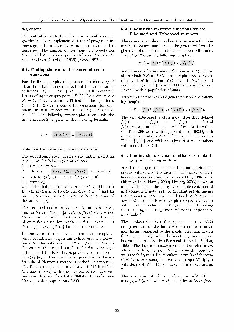
"!$#%&' (')+*( (, (#-.0/1 32,%#- (4#$&456-32 #-%K~2±l|~2~7°lPq«¬P~7|~q ÄqYy| lu>My|P~y|~2PiYy|~³µxlw~q>~2ll Ky| lux| ³±ll| y|P¯xlwH~2~2u P ~2~2uhy|~q u>y|P~ a P|l±l" uP±iuP±lx±l~ux;y|~2PiYy|~qwxl~H~2~2uSP|~qw~2uhy|~q; u¥y|PiwiuP±lx±l~lS«¬P~uBPH~2>® y|~2"Yy| luxw>uxOHlPPiYy| luw Ä2~c~2|~"Phw~2u>B>u~äKH~2| ~2uhy"H¬xlw~q>luxY³"~y|~2"w°|lÈ·7liKH~2|±xMÊq¡lËl¡hÎiÈ@ð®lÄqPHÊq¡l¡hñlÎ
U@G*Q*U@G*AqL*?YEME EqL*? q?lEHG*Q"EYQ*??*IqU@EHG
hPly|P~´Ðx"wzy~äPP ~ly|P~DP|K~qw|w|~qKiw|Yl~2|O ±ll| y|P>w>°lÐxuxK uP±Vy|P~²|By"w)y|P~´w~qluxB³µl"K~2~qÇhxYy| luxw2ò Ú ÈkjnÎVÒ n-j R _ W%j _ Ò OiwP|~qw~2uhy|~q^M~y®ñ > uPPKy³µlKy|PKy7x "w W ã á Þ|ß á j H~±l l~2uMx¢P~2|~ã á Ò È n á ÞW á Þ á Î|~>y|P~B~ ~2uhy"w¢y|P~~qÇhxYy| luxw2ß á Ò ÈBÊ á Þñ á Î|~²|By"wy|P~D~qÇhxYy| luxwDÈg°l$w ³P i yzl*c~¢ cluxwiK~2)luP |~q|By"w"ÎÊåØæ)å¯çèç6ÒÉñ P$«¬P~°l Y¢ uP±yzcy|~2PiYy|~qw|~xw~q^òy|P~Ðx"wzy¬y|~2PiYy|~) Q iw¬±l l~2ulwcy|P~®°l Y¢ uP±°l|PiPò
Q! R Ò ÚQ È nHÞWÞ Î#" ÚTR È nHÞWÞ ÎS
y|~®y|xYy¢y|P~)PuPBuPY¢u°Puxy| luxw|~®wxlK~q^«¬P~w~qluxy|~2PiYy|~! R Pu)PP|äK >Yy| lu® ±ll| y|Piw¬±l l~2ulwcy|P~®°l Y¢ uP± y|~2"Yy| l~7 BlMòÊ W Ö>ÒS PÌ j Õ Ò j%$'&'(KÌñ Q*EDW j Õ*)PQ Ò ÚQ Èkj Õ Þ Ú Èkj Õ ÎÞ Ú à·Èkj Õ ÎÎÌHÖÒ0Ö _ ÊlÌ j + L*U@=@? ÈÈ Ú à·Èkj Õ Î!Ò-,/.0Êq 0%12Î Í È·Ö32 q l hÎÎÌÏ Y?4YG j Õhj ¢ y|ÀV y|~q0uBPH~2 y|~2"Yy| luxwæ Z52 q l P¢ y|±l l~2uèP|~qiw luèPP|äK >Yy| lu5,62Êq 0%1uxèu uP y|iHl uhy j%$'&'(KM¢ y|èP|K~qKP|~°l82iPiYy| lu²K~2| YYy| l~ Ú à·ÈkjnΫ¬P~´y|~2| ux8uPKK~qw°l$ Q |~´Âe Q Ò W nHÞWÞ Þ a j uxè°l R |~Âe R Ò W j Õ Þ Ú Èkj Õ ÎÞ Únà Èkj Õ ÎÞ a j ¢P~2|~a Oiw²¥w~y²"uxKl%uxYy|P"luxwzy"uhy"w2«¬P~Vw~ylH~2"Yy| luxw²xw~qðlèwBuhy|P~qwiw´y|P~O°l|Pilw²iwçfeèÒ W _ Þ^)ÞoBÞlBÞ m Þ j R j °l¬y|P~)Hy|y|~2PiYy|~qw2tvu y|P~2lw~Ày|P~Ðx"wzyéy|~2PiYy|~'y|P~y|~2PiYy|~³xlw~q~2ll Ky| lux| ±ll| y|P |~qKiw|Yl~2|~qy|P~8°l Y¬³ uP±BuPY¢u°l|PiPò7 Q! R Ò ^ Wlñ n8" m W R ^´Ï-n lñ nHctvuy|P~D2lw~)y|P~Dw~qluxOy|~2PiYy|~²y|P~DKiw|Yl~2|O ±l³| y|P°lPuxOy|P~$°l Y¢ uP±D~äKP|~qw|w luMòWj Õ*)PQ Ò j Õ ^Ú Èkj Õ ÎUl Ú à·Èkj Õ ÎV«¬Piw|~qwP y>l||~qwHluxPw®y|²y|P~BuPY¢u°l|PiO~2¬y|lu9 w$~y|PKéÈ°~y|PKy"uP±l~2uhy"w"Ϋ¬P~Ðx"wzy®|~qwP y7xlwH~2~2u²°lPux²Ygy|~2Êq hñKÊq> y|~2"Yy| luxwÈg°ly| ~;:Y w~q ΢ y|²HlPPiYy| luñ l P«¬P~w~q³lux8|~qwP yxlw\H~2~2u°lPuxYgy|~2ll y|~2"Yy| luxwcÈg°l*y| ~Êq w~q Î8¢ y|HlPPiYy| lu!ñ l P
=< U@G*Q*U@G*AqL*?Y?>4? qU°NH?#'*G@qU@EHG ;µEAqL*? UBEHG*IC>lU¬IPG*QED7YUBEHG*IC>lU¢G*TFB??
«¬P~®w~qlux>~äPP ~7wPYwPY¥y|P~7|~qP"w l~°Puxy| lu°l¢y|P~:h* Hluxl2MuBPH~2"w2uH~8±l~2uP~2"Yy|~q°|lÉy|P~±l l~2u>y|~2PiYy|~®ux>y|P~Ðx"wzy¬~2 ±lhycuBPH~2"wc¢ y| uxK~äÊ)å;æå¥ËPÝ´~)xw~7y|P~®°l Y¢ uP±y|~2PiYy|~lò
Æ>È°æzÎ!Ò Ú?G È@Æ>È ÚQ È°æzÎÎÞ|Æ>È ÚTR È°æzÎÎÎSÝS y|y|P~w~y7!lH~2"Yy| luxwçfe¥Ò W _ Þ^)ÞoBÞl j uxw~ycy|~2| uxiw)ÂeÀÒ W æ"Þ a j y|P~>y|~2PiYy|~³µxlw~q²~2ll K³y| lux| ±ll| y|P'K~ÐxuP~q ÚQ È°æzÎÒæ6^SÊl ÚTR È°æzÎÒÃæ6^Vñux Ú?G Èkj Q Þ j R Î!Ò j Q _ j R Ygy|~2¢ÏxÊlÊ y|~2"Yy| luxw®Èg°l¬y| ~Êñw~q Î8¢ y|HlPPiYy| lul l l P«\| Hluxl2xuBPH~2"wc2u>H~±l~2uP~2"Yy|~q°|l¯y|P~°l Y¬³ uP±y|~2PiYy|~lò
Æ>È°æzÎÒ ÚIH È@Æ>È ÚQ È°æzÎÎÞ|Æ>È ÚTR È°æzÎÎÞ|Æ>È Ú?G È°æzÎÎÎS«¬P~ây|~2PiYy|~³µxlw~q4~2ll Ky| lux|Ø ±ll| y|P.K~ÐxuP~qÚQ È°æzÎ0Òïæ"^éÊl ÚTR È°æzÎ0ÒïæV^¯ñK Ú?G È°æzÎÀÒ æ"^FÀuxÚIH Èkj Q Þ j R Þ j G ÎØÒ j Q _ j R _ j G Ygy|~2;ÏhPÊS y|~2"Yy| luxwÈg°l)y| ~ñ l¡w~q ÎO¢ y|èHlPPiYy| luD¢l l l l P^¢ y|y|P~w~y¢lH~2"Yy| luxwçfeFÒ W _ Þ^ j *w~y¢y|~2| uxiwÂeÉÒ W æ"Þ a j uxO¢ y|¥y|P~$±l l~2uOÐx"wzy>y|~2uSuBPH~2"w¢ y| uxK~ä´Ê®åOæå0Êq P
KJ U@G*Q*U@G*AqL*?Q*U LqIPGl?#'*G@qU@EHGSElU?>*=@IPG%AYIML + UqLSQ*?BAY?B?µE4
hPly|Piw~äPP ~l¢y|P~´Kiwzy"ux~°Puxy| luâ "Piuhy±l"Pxw¢ y|¥K~2±l|~2~Ï´iw|~qYy|~q^V«¬P~ilw|w7 "K³iuhy!uP~yzcl|Kw¬È@c~2|lux^Bl~2 ilw ÍÀø wMxÊq¡l¡-qKÌl$luK³BPY Í $luxBPYYP7ñ l l PÌ ø ¬uP±x7ñ l lhÎPiKwu Hly"uhy|l ~$ uSy|P~²K~qw ±luâux¥ P ~2~2uhy"Yy| luS uhy|~2"luPuP~qy| luèuP~yzcl|Kw2É "Piuhy±l"PM*xB uP±y|P~x"~y||iK~qw|| Ky| luM¬iwK~ÐxuP~qSlw°l Yw2ON?5SA?03K 4927iwuâPuxK |~qy|~qS±l"PKL>È@çèÌY Q ÞY R ÞSSS2ÞY Û Î¢ y|Ã¥w~yuPKK~qw#PïÒ% PÞ2ÊlÞ"ñKÞSSSÞ|ç ^¯Êl®xB uP±æQ" Y Q ÞæQ" Y R ÞSSS2Þæ"=Y Û È°KÀç²Î7uPKK~qw2*lÅl~2uhy®y|~ql"uPKK~®æ"«¬P~uBPH~2"w e4Ò È6Y á ÎÈ@ R2JY Q 2 SSSS2JY Û 2ÉçMlñlÎ|~è±l~2uP~2"Yy|l"wy|P~èÐxuP y|~OH~2 iuñl|lPKy|³l|PPiw>w7luPuP~qy|~qy|y|P~±l"PM) "Piuhy±l"PxwL>È@çèÌ2ÊlÞY R ÞSSSÞY Û Î¢ y|Ãy|P~ViK~2uhy| yz±l~2uP~2"Yy|lq)|~BuPY¢u´lw7 Bl²uP~yzcl|KwÈ@c~2|lux^*l~2 ilw ÍÓø wMÊq¡l¡-qlÎ\«¬P~¬K~2±l|~2~HuPKK~c u "Piuhy*±l"P LâiwñYÜ¢P~2|~ÜViwy|P~K ~2uxw luM®Ý´~¢ luxwiK~27 BluP~y³cl|Kw^¢ y|8K~2±l|~2~!Ïxq· ~l* "Piuhy\uP~yzcl|Kw^By|P~°l|L>È@çèÌ2ÊlÞYÎ1hPl~äPP ~lH "Piuhy±l"P a ÈzÊ2ÏxÌ2ÊlÞ|h΢ y|K~2±l|~2~®ÏxPçÒFÊ2ÏxÞY Q ÒÃÊlÞY R Ò0iwwPY¢u u h* ±xñK«¬P~ Ki~y|~2 L iw K~ÐxuP~q:lwUTHÈ@çèÌ%e!Î Ò>YäCV WXY ìÈZ*Þ[K΢¢P~2|~²ìÈZ*Þ[KÎÈgy|P~]\5$BT249?E_^039?`
32

"!$#%&' (')+*( (, (#-.0/1 32,%#- (4#$&456-32 #-%
* &(' # )
265879BÎciwy|P~) ~2uP±y|wPly|~qwzy¢xYy|H~yzc~2~2uuPKK~qw Zux [ ufLc~q2xw~8y|P~wB~y|| u² "Piuhy"w yiw7~2uPlP±ly|$luxwiK~27y|P~P|lP ~2'!ÐxuxK uP±$wPly³~qwzyxYy|$°|l y|u|P y|"|uPKK~ [H«¬P~Kiwzy"ux~°Puxy| lu¥°luPKK~qw èux [; uâ "Piuhy a È·ñ l PÌ2ÊlÞYÎç¶ÒÀñ l PK°l ;2HY 2SçMlñux A2 [62âçMlñiwwPY¢u u h* ±x!P
#"$&( #" &(' # "!#)
hPlÐxuxK uP±y|P~Kiwzy"ux~)°Puxy| lu´ìÈ@ PÞ[K΢c~8¢ luK³wiK~2y|P~8°l Y¢ uP±luxwiK~2"Yy| luMdhPl®uBuPKK~%$Øc~K~ÐxuP~ _ Y´ux ^ Y´ uPKw°|l uPKK~&$¶K~2H~2uxK uP±Olu¢P~y|P~2y|P~2è|~xw~qDy|²±l$y|uPKK~´È'$ _ YÎvîí?T´ç
È° u$ K"B¢iw~®K |~qy| luHÎl8È'$ ^ YÎvîí?Tç È° u$lPuhy|~2³ K"B¢iw~K |~qy| luHÎB i| l\c~>K~ÐxuP~ _ Ê>uxb^)Ê uPKw2èy|~y|xYy uO "Piuhy±l"Pxw²wPly|~qwzyxYy|°|lÓ 8y|_[>clPiH~®xw uP±Yy¬hwzy¬~2 y|P~2)È _ YlÞ _ ÊÎ!lÈ _ YlÞ^)ÊÎ!l®ÈF^ YlÞ _ ÊÎ!l)ÈF^ YlÞ^)ÊÎ! uPKw2«¬P~2|~°l|~°P³y|P~27c~8¢ luxwiK~27wx"lP uxYy| luxw! uPKwluP lM~yèÈ _ YlÞ _ Êε³µxYy|âH~èVxYy|â°|l% Vy|][¥xw uP± _ Yux _ Ê$ uPKwluP l hPly|P~2lP uxYy| luxw>) uPKwc~²K~ÐxuP~y|P~´ux l±llxwuPy"Yy| luxw2FtvuS¢xYy°l Ywjl*Y7Ò)( jl*Y#*h(j,+1Y®Ò j$îí?TXYltvul"K~2cy|±ly|uPKK~8[°|lÉ B~quxwc\°lP¢Hhwz³w P ~)¬Kwcc~®xl~y|>xw~
ÊÎ²È _ YlÞ _ Êε³µxYy|Mò*xw uP±_[l*Y7uBPH~2¢ _ Y7 uPKw¬ux[-+1Y)uBPH~2¢ _ Ê® uPKw2Ì
ñlÎ²È _ YlÞ^)Êε³µxYy|Mò!xw uP±A[l*Y _ Ê)uBPH~2 _ Y) uPKwux Y1^[-+1Y)uBPH~2¢Y^)Ê® uPKw2Ì
hβÈF^ YlÞ^)Êε³µxYy|MòOxw uP±ÃÈ@ç ^ [KÎUl*YDuBPH~2$W^ Y uPKwux´È@çB^[KÎ"+1Y8uBPH~2¢Y^)Ê7 uPKw2Ì
ÏBβÈF^ YlÞ _ Êε³µxYy|Mò\xw uP±È@ç>^6[KÎUl*Y _ Ê¢uBPH~2cp^ Y uPKwux Y^¥È@ç ^[KÎ"+1Y)uBPH~2¢ _ Ê® uPKw2
«¬Piwl||~qwHluxPwy|8luP~ Bly|"l~2 ~q u K"B¢iw~K ³|~qy| luuxluP~8 Bly|"l~2 ~q u²lPuhy|~2" K"B¢iw~)K ³|~qy| luÈ Z!Òâ hÎ7~2uP~2" Ä2 uP±)y|Piw!P|K~qw|w°l Zc×¥ Plc~lKy" u°l¢uPKK~ [ò
ÊÎ )È _ YlÞ _ Êε³µxYy|xw2ò>xw uP±¥È[ _ Zzç²ÎUl*YuBPH~2_ Y® uPKwux´È[ _ Zzç²Î"+1Y)uBPH~2¢ _ Ê® uPKw2ÌñlÎ ^È _ YlÞ^)Êε³µxYy|xw2ò^xw uP±È[ _ Zzç²ÎUl*Y _ ÊcuBPH~2_ Y7 uPKw¬uxdY`^;È[ _ Zzç²Î"+1Y7uBPH~2¬`^)Ê uPKw2ÌhÎ \ÈF^ YlÞ^)Êε³µxYy|xw2òMxw uP±ÈÈ Z _ ÊÎzç ^;[KÎUl*Y¬uBPH~2^ Y uPKw®uxOÈÈ Z _ ÊÎzç ^ [KÎ"+1YuBPH~2®^)Ê uPKw2Ì
ÏBÎ nÈF^ YlÞ _ Êε³µxYy|xw2òMxw uP±ÈÈ Z _ ÊÎzç ^ [KÎUl*Y _ ÊuBP³H~2¢+^ Y7 uPKw¢uxdY`^;ÈÈ Z _ ÊÎzç ^#[KÎ"+1Y®uBPH~2 _ Ê7 uPKw2
y|~>y|xYyH~q2xw~cy|P~wB~y||² "Piuhy"w®y|P~ÈF^ YlÞ _ ÊÎcuxDÈF^ YlÞ^)Êε³µxYy|xw°|lÉ y|;[ _ Zzç¶2uH~"xuP±l~q´y|$y|P~´È _ YlÞ^)ÊÎ)uxâÈ _ YlÞ _ Êε³µxYy|xw2*|~qwH~q³y| l~2 lB°|l y|uPKK~È Z _ ÊÎzçB^[H Zc×O Ptµyiw!uP~q~qw|w||)y|)Ðxuxy|P~wPly|~qwzy!xYy|xw!M Ky|P~¢°lPyzBH~qw¬uxy|P~)wPly|~qwzyc^y|P~7°lPc¢ n±l l~xw¬8±l lxwPly|~qwzy7xYy|H~yzc~2~2u´ ux[H)«¬P~uBPH~27 BlxwZ 2 Y®H~q2xw~8[-+1Y 2 Y®°luB åR[A2¥çè¬lw~q´luèxl"B±l|lPux²BuPY¢ ~qK±l~ "Piuhy8P|lH~2³y| ~qw!y|P~°l Y¢ uP±)y|~2PiYy|~7Â¥°l!y|P~®Kiwzy"ux~°Puxy| lu
33

"!$#%&' (')+*( (, (#-.0/1 32,%#- (4#$&456-32 #-%TlæY#Z!ÒSìÈ@ PÞ[KÎc "Piuhy a È@çèÌ2ÊlÞYÎiw¢xw~q^òÊ U@G% ZÞ"ÖnÞ"ÖPñKÞYÞñKÞ TxÞ TxÊlÞ TBñKÞ TlæY#ZÒâçèÌñ µE È ZÒâ PÌZ72 YlÌZ!Ò Z _ ÊÎ W Ö>ÒÃÈ[ _ Z<ocç²ÎUl*YlÌ)ÒFÈ[ _ Zocç²Î"+1YlÌÏ ÖPñ8ÒÃÈÈ Z _ ÊÎ(o\ç>^3[KÎUl*YlÌñ8ÒÃÈÈ Z _ ÊÎ(o\ç>^3[KÎ"+1YlÌq TxÊ7Ò ÚQ È·ÖnÞYÞY΢ÌTBñ8Ò ÚQ È·ÖPñKÞñKÞYÎ¢Ì TÒ TVU@G ÈTxÊlÞ TBñlÎÌ U ÈTlæY#Z . TBÎSTlæY#Z!ÒETxÌ j: Y?4YG TlæY#Ztvuy|P~ uP~8Ê¢ny|P~¢y|~2PiYy|~¢y|P~uP~2~qK~q K2PY|iP ~qw|~K~ÐxuP~q^*tvu)y|P~c uP~¬ñ¢c~xl~y|P~clH~2"Yy|l µE ¢ y|y|P~ y|~q>uBPH~2^ BlxwRZ 2 Yltvu>y|P~ uP~qw8uxÏy|P~¢Y|iP ~qw!Öux_®K~ÐxuP~¬y|P~¢uBPH~2"w _ Y¢ux _ Ê uPKw2|~qwH~qy| l~2 l*°lxYy|è°|ló y|F[D u; K"B¢iw~K |~qy| luMux^w i| l\y|P~Y|iP ~qw8ÖPñ$ux ñ$K~³ÐxuP~¬y|P~¬uBPH~2"w6^ Y¢ux _ Êc uPKw°lxYy|°|lØ y|[ u´lPuhy|~2" K"B¢iw~8K |~qy| luM7tvuy|P~ uP~qKH°ly|P~P||~2uhy BlVZ!y|P~PuxK~ÐxuP~q;°Puxy| lu ÚQ È·ÖnÞYÞYÎxlwy|2iPiYy|~®y|P~8 ~2uP±y|#TxÊ)y|P~wPly|~qwzyxYy|°|l y| [ u K"B¢iw~K |~qy| luMKux^Bw i| l ÚQ È·ÖPñKÞñKÞYÎ2iPiYy|~qw¢y|P~ ~2uP±y|FTBñ>y|P~wPly|~qwzyxYy| u´lPuK³y|~2" K"B¢iw~¢K |~qy| luM*tvuy|P~¢ uP~7y|P~¢ ~2uP±y|;TÈTlæY#ZÎ\y|P~8wPly|~qwzy¬xYy|°|lÉ y| [>°lcy|P~8P||~2uhy¬ BldZÈg°l® * Blxw Zzà 2HZÎiw7K~ÐxuP~q^®tvuy|P~ uP~;:c~xl~y|P~)|~qwP yqò TlæY#ZÒâìÈ@ PÞ[KΫ¬P~ y|~2| uxéuPKK~qw¶°l y|P~ PuxK~ÐxuP~q °Puxy| luÚQ Èkj Q Þ j R Þ j G Îc|~ K2nY|iP ~qw W ÖnÞ"ÖPñKÞYÞñ j B±l lxW Y j ux W a j È@w~y\K"uxKl0uxYy|P"lluxwzy"uhy"w"Î\«¬P~w~y®lH~2"Yy| luxwxw~q°l®wBuhy|P~qwiw7!y|P~°l|Pi ÚQiw¢çfeèÒ W _ Þ^)Þ unÞ ( j-* j hPly|Piw y|~2PiYy|~ y|P~ y|~2PiYy|~³µxlw~q ~2ll Ky| luK³| ±ll| y|P °lPux y|P~ °l Y¢ uP± ~äKP|~qw|w luMòÚQ Èkj Q Þ j R Þ j G βÒó u\ÈÈkj Q _ j R ÎÞqÈkj Q _ Ê _ j G ^ j R ÎΫ¬P~D°Puxy| lu ÚQ È·ÖnÞYÞYÎ2iPiYy|~qwy|P~è ~2uP±y|y|P~wPly|~qwzycxYy|°|lé )y|_[ u K"B¢iw~K |~qy| lulw!y|P~ uP Pé^y|P~7 ~2uP±y|xw7È·Ö _ ÎuxÈÈ·Ö _ ÊÎ _ È6Yp^ ÎÎ;y|P~ È _ YlÞ _ Êε³âux È _ YlÞ^)Êε³µxYy|xw2V|~qwH~qy| l~2 lux^Pw i| lhy|P~7°Puxy| lu ÚQ È·ÖPñKÞñKÞYÎc2iPiYy|~qwy|P~ ~2uP±y|S)y|P~´wPly|~qwzyxYy|S°|l Dy| [O uâlPuhy|~2³ K"B¢iw~)K |~qy| luèÈ°Hy|°l¢y|P~8P||~2uhy Bl ZÎc«¬P~|~qwP y>xlwH~2~2uO°lPuxV°ly|P~$±l l~2u¥¡l¡² uPPKy³µlKy|PKyx "w W [HÞ|ìÈ@ PÞ[KÎ j Êå [VåØ¡l¡P^°l8±l"P a È·ñ l PÌ2ÊlÞYÎYgy|~2$Êñ: y|~2"Yy| luxwÈg°l>y| ~²ñ:Y ´w~q ÎÉ¢ y|S´HlK³PiYy| luâ:q l P¯«¬P~Dl||~qy|uP~qw|w°llPKy"Yy| luây|P~;Kiwzy"ux~D°Puxy| luFìÈZ*Þ[KÎ> "Piuhyxlw~q0luy|~2PiYy|~Ââux°l|Pi ÚQ ¬lw!P|Yl~q~äKH~2| ~2uhy" uxy|P~2l|~y|i2 l«¬P~PPH~2c~qwzy| >Yy|~ Z¢È°~qÇhxxy|1Y u>y|P~ uP~®ñ®^y|P~HYl~y|~2PiYy|~ά2uH~8K~q|~qlw~q^
?BTVTVI E 903.EA 7 ^GK 77M;B 5S9 2 E 4K (7AT5S2 .\ER95S9d2 E \5$BT249?ES^039?265879 2 E]K 5S9E 7 ^\2 E!47DE2E. MK 42E .!4 972E?EE!\12 E ^7KSK 7I 5S9XD4K 0EU (zÈ6YTlñ _
ÊÎUl(°çMl*Y#**w|~qwP y¢c~®xl~
?BTVTVI < E ?7. M0324265879 7 ^!2 E6\5$BT249?E ^039?265879ìÈ@ PÞ[KÎ* å][32¥ç^7A\K 77M 9E26I 7A a È@çèÌ2ÊlÞYÎ4CB#E!\79 2E. MK 42E ^7AT.103K 4 ÚQ 49%\ I 5S2 2 E 903.EA 7 ^K 77M;B_\ER9E!\ !1_`E.1.!4 "!5$B]?7ATAE?2
«¬Piwc ±ll| y|Pé2uH~xw~q>y|wl l~y|P~2cP|lP ~2>w u BlDuP~yzcl|Kw®K~2±l|~2~>Ïxwx"èlw®y|P~|lKy| uP±$P|lK³ ~2 !ÐxuxK uP±$wPly|~qwzy®xYy|²H~yzc~2~2u²yzcuPKK~qw2^lÐxuxK uP±y|P~>Ki~y|~27c±l"PM"hPl®wl B uP±y|P~Ðx"wzyP|lP ~2' y)iw®w ~2uhy®y|wzy|l|~uBPH~2"w¬wzy|~2xw®uxw ±luxwyzc´±l~2uP~2"Yy|l"w8±l B uP±´´wPly|~qwzyxYy|; y|P~lH~2"Yy| lu]TlæY#ZÒ TD¬lw|~q Ä2~qV u;y|P~$ uP~$´y|P~HYl~y|~2PiYy|~)Â8tvu È@$PBPlxlKBhh Í B uPxP²Êq¡l¡-qK̲"huxu ÍöxYy||uBlÊq¡l¡:BÌ¢lPi Í$# ~2|YBuP n®ñ l l hÎy|P~V ±l³| y|P>wÐxuxK uP±wPly|~qwzyxYy|H~yzc~2~2u²uBx uPKK~qw uâ BlSuP~yzcl|KwK~2±l|~2~$ÏO|~±l l~2uMØ«¬P~HYl~¢ ±ll| y|PF±l~2uP~2"Yy|~qB8y|P~¢y|~2PiYy|~³µxlw~q~2l³ Ky| lux| ±ll| y|P K ôn~2"w¢°|l \BuPY¢u$ ±ll| y|P>wux y"w¢~qwzy| >Yy|~)iw¬uPycl"w~l
% ¹& ¼ » ª ? ¾¦B¿z¼ » ¦«¬P~ |~2P|~qw~2uhy|~q6y|~2PiYy|~³µxlw~q ~2ll Ky| lux| K³P|hl"ÃxlwH~2~2uØxw~qFwx2~qw|wz°P 0y|ÀKy|l>Yy|i2 uBl~2uhy)lPKy"Yy| lux ±ll| y|P>w®ux$°l)Kiw|Yl~2|>Yy|P~2>Yy|i2H°l|Pilw°lcy|P~®±l l~2uPYy"w~y"w¬ux°ly|P~±l l~2u ±ll| y|P 9 w*y|~2PiYy|~qwÈ°~l ±x* y|~2"Yy| luxw2|~qP³w luxw2 Blxw\ux8K ~qw"ÎY¢Pi"K~qw|| H~y|P~¬w|2uPuP uP±y|P~lP ~äPYy"®wzy||xy|P|~qw¢È°>Yy|| äK~qw2l|"Kw2±l"Pxw2y||~2~qw"Îux¢Pi"luhy" u>y|P~7°l|Pi)y|~2PiYy|~qwc uy|P~HKKl!«¬Piw¢PP|hl"2uH~)xw~q°l¢wBuhy|P~qwiw¬*uP~2 ±ll| y|P>w2l°Puxy| luxw2KKK~2iw¬uxwl Ky| luxw2h¢Pi"Yg³y|~2|¬"Pw2uOH~y|P~2l|~y|i2 è uBl~qwzy| ±hYy|~q;ux²Åzxwzy| ³Ðx~q^
e 9H%9 ¨ 9\» ª 9 ¦l ~lè®ÈzÊq¡lËl¡hÎ N K (7AT5S2 .158?(')EK E279 B#U ';26AT0?2603AE!\* 494+(E.!E92 7 ^-, 4A4KSK EK/.R7. M0324265879«¬P~V$tz«!|~qw|w2
$ |~2uPlYn8 Í $ |~2uPlYYP«®ÈzÊq¡l¡lhÎ¥$P y| ~qKiBl~2 ~y|luxwuxKh* ÐH2Yy| luâ$~y|PKPw20, A7?1]7 ^ E QR5SABT232T92EAT942658794K.R79^EAE9?E/794`5$BT04K52T9`^7AT.!42658796'7CBT2E.]B¢È°PM(qË98K:Î;:iy|l|i suP l~2"w yzl$~2 HlP|uP~lPxwzy|" iP
®>PYO ø ~2 ¢) 5<llPuxwluMc) Í : iw|wiK~qw2=<xÈzÊq¡l¡ÏBÎ?>1ETBT5 *90, 4262EAT9 B#UA@ K E.!E928B=7 ^CB E0B#4K E
34

"!$#%&' (')+*( (, (#-.0/1 32,%#- (4#$&456-32 #-%[ #E?2 ` [ AT58E92E!\' 7 ^26I 4AE1¯PKiwluK³µÝ´~qw ~2l¢~qlB³ uP±xP8
7liKH~2|±x OÉÈzÊq¡lËl¡hÎ E9E2658? N K (7AT5S2 .]B5S9 ' E4A? [ M265S.15 4265879 49%\0* 4? 5S9EG_`E4AT95S9PKiwluK³µÝ´~qw ~2lP¢~qlK uP±xP8
ð®lÄqP <xcÈzÊq¡l¡hñlÎ E9E2658?, A7*A4.1.15S9DcP|iK±l~l«¬P~8$tz«0!|~qw|w2
uxK|~lKÈzÊq¡l¡ÏBÎKy|l>Yy|i2 )K~ÐxuP~q®°~qYy|P|~qw2òM«¬P~w P y"uP~2lxw¬~2ll Ky| lu!ñ³vK ~2uxw luxH°~qYy|P|~)K~³y|~qy|l"w\ux8 ±ll| y|P0°l*xw uP±y|P~2htvuð¬ð® uPuP~qÈ O^ Î4N \D49?ETB]5S9 E9E2658?3, A7*A4.1.15S9È°PMnÏ:>:q³Ïh¡ÏBÎP$tz«0!|~qw|w÷Yc"lB°l">cBlKw2
±lPl~2uMB«® Íø xuP±xB«®nÈzÊq¡l¡ÏBÎ$O!ll YP ~âKK~2 ³ uP±°l7KK~2 ³µxlw~q$lKÅz~qy®|~ql±luP y| lu²wKwzy|~2>w2®tvuðÃð® uPuP~qÈ O^ ÎSN \D49?ETBd5S9 E9E2658? , A7*A4._`.15S9>È°PMPÏq¡Y³µÏ: qlÎB$tz«À!|~qw|w÷Yc"lB°l">cBlKw2
M~2~lÝà ø i<x Í MPux^ ø ø PÈzÊq¡l¡lhÎK ø BP|i®¬÷®'PP|hl"O°ll~2ll B uP±;luhy||l ~2"wux¢lHy®cKK ~qwy|"P ~2l~:h* y|uP~qw|w³BH~q Ðx~q²«*lwKw2, A7?1 7 ^ 2@ @ @ 2T92EAT942658794K .R79^! 79 @ D7K 032658794A .R7. M0324265879x!tFO+O+OO!|~qw|w2
öiw|wluM9<xq)hÈzÊq¡l¡lËhÎlPPiYy| lu7>ux±l~2~2uhy^°l*Ky|³>Yy|iK~qw ±lu>\ ±ll| y|P>wy|P|lP±l>~2ll Ky| luM , A7?17 ^32@ @ @ 2T92EAT942658794K .R79^EAE9?Ed79@ D7K 032658794A .R7. M0324265879x!tFO+O+OO!|~qw|w2
$luxBPYnö Í $luxBPYYPO®È·ñ l lhÎFuÀ ±l³| y|PÀ°liw|Yl~2|P~20hx ~qw\HöKy| >B¢~2±³Pi¢~yzcl|Kw2 , A7?1 7 ^ C2 2T92EA+ .R79^! 79 >\5$B#?7D`EA ' ?58E9?E/ >'- 9¥ö7yqMÊ?:q³zñ PKñ l lPPKPHl|x<hxuMMM~qy|P|~>y|~qw7 uDy| ÐHitvuhy|~2 ±l~2ux~lMll·ñËÏhP¢È°PM!ñYÏlϳzñqYÏBβBP| uP±l~2³ :~2|i±xc~2| u ø ~2 ³K~2 H~2|±x
c~2|lux^<x ³ hl~2 ilw2Thc ÍSø wM hcKÈzÊq¡l¡-qlÎiwz³y|| PKy|~q BllPKy|~2¢uP~yzcl|Kw2ò*wP|l~2l , 4A*`4KSK EK>\5$BT26AT5032E!\ .R7. M032 Pnñ18nÊq P
$luxBPYnPö Í $luxBPYYPO^È·ñ l l hÎ , 4A4KSK EK '7CB*`2E.]B\I 5S2 >\5$BT26AT5032E!\* E.!7A U';26AT0?2603AETB\49%\ [ A*`(495 4265879 7 ^ 2T92EA4?265879 BYlhw P "wn®K'7!PP·\È° u$¢xw|wiuHÎ
ø ¬uP±x hc ðKÈ·ñ l lhÎK¥wP|l~2®luP y| ³µ BluP~yzcl|Kw2 E7AE2658?4K .R7. M032EA ' ?58E9?EHñ l lP\Êq :+8nÊñKÊl
$PBPlxlKBhhP8ð Í B uPxP7 ÈzÊq¡l¡-qlÎ hxP y³y|l ~2"uhy!|lKy| uP±8 uKiwzy|| PKy|~q Bl>uP~yzcl|Kw2 2@ @ @ A49 B+ .R7. M032 "!Y\Ê2Ïqlñ18nÊ2ÏqP
"huxuMY! Í öxYy||uBl <xPÈzÊq¡l¡:ÎHlxly|lKy| uP±lu´"Pl"P\| uP±hwcK~2±l|~2~)°lPq®tvuMð®| Äqux8ux
hÝSiK>l~2qnÈ O^ Î7';5SA7??72!c| ~y|luK ~2uhy| ÐHÊñq18nÊq:B
¢lPiK7 Í # ~2|YBuP n <x^È·ñ l l hÎM$ uP PÉñ³·y|~2| ux|lKy| uP± u$ñ³ ÅzP$ "Piuhy¬±l"Pxw2 .R7. M032EAB]49%\N AT265 ?584K72T92EKSK 5 (E9?E ") "YH:+8BÏhP
35


Kernels on Prolog Proof Trees: Statistical Learning in the ILPSetting
A. Passerini passerini a©dsi·unifi·it
P. Frasconi p-f a©dsi·unifi·it
Dipartimento di Sistemi e Informatica, Universita degli Studi di Firenze
L. De Raedt deraedt a©informatik·uni-freiburg·de
Institute for Computer Science, Albert-Ludwigs Universitat, Freiburg
Abstract
We develop kernels for measuring the similar-ity between relational instances using back-ground knowledge expressed in first-orderlogic. The method allows us to bridge thegap between traditional inductive logic pro-gramming representations and statistical ap-proaches to supervised learning. Logic pro-grams will be used to generate proofs of givenvisitor programs which exploit the avail-able background knowledge, while kernel ma-chines will be employed to learn from suchproofs. We report positive empirical resultson Bongard-like and M -of-N problems thatare difficult or impossible to solve with tra-ditional ILP techniques, as well as on a realdata set.
1. Introduction
Within the field of automated program synthesis, in-ductive logic programming and machine learning, sev-eral approaches exist that learn from example-traces.An example-trace is a sequence of steps taken bya program on a particular example input. For in-stance, Alan Bierman (Biermann & Krishnaswamy,1976) has sketched how to induce Turing machinesfrom example-traces; Mitchell et al. have developedthe LEX system (Mitchell et al., 1983) that learnedhow to solve symbolic integration problems by an-alyzing traces (or search trees) for particular exam-ple problems; Ehud Shapiro’s Model Inference System(Shapiro, 1983) inductively infers logic programs byreconstructing the proof-trees and traces correspond-ing to particular facts; and Zelle and Mooney (Zelle& Mooney, 1993) show how to speed-up the executionof logic programs by analyzing example-traces of theunderlying logic program. The diversity of these ap-plications as well as the difficulty of the learning tasks
considered clearly illustrate the power of learning fromexample-traces for a wide range of applications.
In the present paper, we generalize the idea of learningfrom example-traces. Rather than explicitly learninga target program from positive and negative exampletraces, we assume that a particular – so-called visitorprogram – is given and that our task consists of learn-ing from the associated traces. The advantage is thatin principle any programming language can be used tomodel the visitor program and that any machine learn-ing system able use traces as an intermediate represen-tation can be employed. In particular, this allows us tocombine two frequently employed frameworks withinthe field of machine learning: inductive logic program-ming and kernel methods. Logic programs will be usedto generate traces corresponding to specific examplesand kernels will be employed for quantifying the sim-ilarity between traces. The combination yields an ap-pealing and expressive framework for tackling complexlearning tasks involving structured data in a naturalmanner. We call trace kernels the resulting broad fam-ily of kernel functions obtainable as a result of thiscombination. The visitor program is a set of clausesthat can be seen as the interface between the avail-able background knowledge and the kernel itself. In-tuitively, visitors are employed to specify a set of usefulfeatures and in this sense play a role similar to rmodesin ILP.
Starting from the seminal work of Haussler (Haus-sler, 1999), several researchers have already proposedkernels on discrete data structures such as sequences(Lodhi et al., 2000; Jaakkola & Haussler, 1998; Leslieet al., 2002; Cortes et al., 2004), trees (Collins &Duffy, 2002; Vishwanathan & Smola, 2002), annotatedgraphs (Gartner, 2003; Scholkopf & Warmuth, 2003),and complex individuals defined using higher orderlogic abstractions (Gartner et al., 2004). Construct-ing kernels on structured data types, however, is notthe only aim of the proposed framework. In many
37
Kernels on Prolog Proof Trees: Statistical Learning in the ILP Setting
symbolic approaches to learning, logic programs allowus to define background knowledge in a very naturalway. Similarly, in the case of kernel methods, the no-tion of similarity between two instances expressed bythe kernel function is the main tool for exploiting theavailable domain knowledge. It seems therefore nat-ural to seek a link between logic programs and ker-nels, also as a mean for embedding knowledge intostatistical learning algorithms in a principled and flex-ible way. This aspect is an important contributionof this paper as few alternatives exist to achieve thisgoal. Propositionalization, for example, transformsa relational problem into one that can be solved byan attribute-value learner by mapping data structuresinto a finite set of features (Kramer et al., 2000). Al-though it is known that in many practical applicationspropositionalization works well, its flexibility is gener-ally limited. A remarkable exception is the methodproposed in (Cumby & Roth, 2002) that uses descrip-tion logic to specify features and that has been subse-quently extended to specify kernels (Cumby & Roth,2003).
The guiding philosophy of trace kernels is very dif-ferent from the above approaches. Intuitively, ratherthan defining a kernel function that compares twogiven instances, we define a kernel function that com-pares the execution traces of a program (that ex-presses background knowledge) run over the two giveninstances. Similar instances should produce similartraces when probed with programs examining char-acteristics they have in common. Clearly these char-acteristics can be more general than parts. Hence,trace kernels can be introduced with the aim of achiev-ing a greater generality and flexibility with respect toconvolution and decomposition kernels. In particular,any program to be executed on data can be exploitedwithin the present framework to form a valid kernelfunction, provided one can give a suitable definition ofthe visitor program to specify how to obtain relevanttraces and proofs to compare examples. In addition,although in this paper we only study trace kernels forlogic programs, similar ideas could be used in the con-text of different programming paradigms and in con-junction with alternative models of computation suchas finite state automata or Turing machines.
In this paper, we focus on a specific learning frameworkfor Prolog programs. Prolog execution traces consistof sets of search trees (see e.g. (Sterling & Shapiro,1994)) associated with goals in the visitor program;these traces can be conveniently represented as Pro-log ground terms. Thus, in this case, kernels overtraces reduce to Prolog ground terms kernels (PGTKs)(Passerini & Frasconi, 2005). These kernels (which are
briefly reviewed in Section 3.3) can be seen as a special-ization to Prolog of the kernels between higher orderlogic individuals earlier introduced in (Gartner et al.,2004).
The paper is organized as follows. In Section 2 we re-vise the classic ILP framework and describe the struc-ture of visitor programs. In Section 3 we describe thegeneral form of the kernel on logical objects and, inparticular, Prolog proof trees, in Section 4 we givesome implementation details, and finally in Section 5we report an empirical evaluation of the methodologyon some classic ILP benchmarks including Bongardproblems, M of N problems on sequences, and muta-genesis.
2. Visitors and proof trees in FirstOrder Logic
In traditional inductive logic programming ap-proaches, the learner is given a set of positive andnegative examples P and N (in the form of definiteclauses that are (resp. are not) entailed by thetarget theory), and a background theory BK (a setof definite clauses), and has to induce a hypothesisH (a set of definite clauses) such that BK ∪ Hcovers all positive examples and none of the negativeones. More formally, ∀p ∈ P : BK ∪ H |= p and∀n ∈ N : BK ∪H 6|= n. In practice, rather than work-ing with ground clauses of the form e ← f1, ..., fn asexamples, inductive logic programming systems oftenemploy e as the example and add the facts fi to thebackground theory BK. As an illustration, considerthe famous mutagenicity benchmark by (Srinivasanet al., 1996). There the examples are of the formmutagenic(id) where id is a unique identifier of themolecule and the background knowledge containsinformation about the atoms, bonds and functionalgroups in the molecule. A hypothesis in this casecould be
mutagenic(ID)← nitro(ID,R), lumo(ID,L), L< -1.5.
It entails, i.e., covers, the molecule listed in Fig. 1.For the purposes of this paper, it will be convenientto look at examples as objects and to considerthe clausal notation h(x) ← f1, ..., fn where x is aunique identifier of the example. Furthermore, wherenecessary, we will refer to the head of the example ash(x) and the set of facts in the body as F (x).
We can now introduce the framework of learning fromtrace kernels. The key difference with the traditionalinductive logic programming setting is that the learneris given a set of so-called visitor clauses V , which de-
38

Kernels on Prolog Proof Trees: Statistical Learning in the ILP Setting
mutagenic(225).molecule(225).logmutag(225,0.64).lumo(225,-1.785).logp(225,1.01).nitro(225,[f1_4,f1_8,f1_10,f1_9]).atom(225,f1_1,c,21,0.187).atom(225,f1_2,c,21,-0.143).atom(225,f1_3,c,21,-0.143).atom(225,f1_4,c,21,-0.013).atom(225,f1_5,o,52,-0.043)....
Figure 1. An example from the mutagenesis domain
fine visitor predicates and which replace the hypothe-sis H. So rather than having to find a set of clauses H,the learner is given a set of clauses V . The idea thenis that for each example x, the proofs of the visitorpredicates are computed. These proofs then consti-tute the representation employed by the kernel, whichhas to learn how to discriminate the set of proofs fora positive example from those of a negative example.The rationale behind the use of the program trace isthe idea that not only the success or failure of the goalis of interest in order to characterize a given instance,but also the full trace of steps passed in order to pro-duce such a result. Different visitors can be conceivedin order to explore different aspects of the examplesand include multiple sources of information.
This idea can be formalized as follows: for each exam-ple (h(x), F (x)), background theory BK and visitorclauses V defining visitor predicates vi, we computethe set of proofs Pi(x) = p | p is a proof such thatBK ∪ F (x) ∪ V |= vi(x).
So far, we have not detailed which type of proof ortrace is employed. At this point, there are severalpossibilities. One could employ the SLD-tree, whichwould not only contain information about succeedingproofs but also about failing ones. The SLD-tree ishowever a very complex and rather unstructured rep-resentation. It is much more convenient to work withand-trees for the visitor facts.
An and-tree for a query v for an example (h(x), F (x)),a background theory BK and visitor clauses V forwhich F (x) ∪BK ∪ V |= v is a tree such that
• v is the root of the tree and
• if v is a fact in F (x) ∪BK ∪ V then v is a leaf
• otherwise there must be a clause w ← b1, ..., bn ∈BK ∪ V and a substitution θ grounding it suchthat wθ = v and BK ∪ V |= biθ∀i and there is
a subtree of v for each biθ that is an and-tree forbiθ
The simplest visitor we can imagine just ignores thebackground knowledge and extracts the ground factsconcerning a given example (or a subset of them).Note that visitors actually allow us to expand the ex-ample representation as described in (Lloyd, 2003) bynaturally including information derived from the back-ground knowledge.
As an example, consider again the mutagenicity bench-mark. The following is the atom bond representationof the simple molecule in Figure 2. By looking at themolecule as a graph where atoms are nodes and bondsare edges, we can introduce the common notions ofpath and cycle:
1 : cycle(E,X):- 2 : path(E,X,Y,M):-path(E,X,Y,[X]), atm(E,X,_,_,_),bond(E,Y,X,_). bond(E,X,Y,_),
atm(E,Y,_,_,_),\+ member(Y,M).
3 : path(E,X,Y,M):-atm(E,X,_,_,_),bond(E,X,Z,_),\+ member(Z,M),path(E,Z,Y,[Z|M]).
A possible visitor in such context would be the onesimply looking for a cycle in the molecule, which canbe written as:
4 : visit(E):cycle(E,X).
Note that we numbered each clause in BK ∪ V (butnot in F (e)1) with a unique identifier. This will allowus to take into account information about the clausesthat are used in a proof.
In many situations, the and-tree for a given goal willbe unnecessary complex in that it may contain severaluninteresting subtrees. To account for this situation,we will often work with pruned and-trees, which aretrees where subtrees rooted at specific predicates (de-clared as leaf predicates by the user) are turned intoleafs. This will allow the kernel to ignore the wayatoms involving these predicates are proved. For in-stance, consider again the molecule in Figure 2, andsuppose we have the background knowledge of func-tional groups as described in (Srinivasan et al., 1996).A potential visitor could look for a benzene ring withinthe molecule, and eventually find out the details of the
1These numbers would change from example to exampleand hence, would not carry any useful information.
39

Kernels on Prolog Proof Trees: Statistical Learning in the ILP Setting
atm(d26,d26_1,c,22,-0.093).atm(d26,d26_2,c,22,-0.093).atm(d26,d26_3,c,22,-0.093).atm(d26,d26_4,c,22,-0.093).atm(d26,d26_5,c,22,-0.093).atm(d26,d26_6,c,22,-0.093).atm(d26,d26_7,h,3,0.167).atm(d26,d26_8,h,3,0.167).atm(d26,d26_9,h,3,0.167).atm(d26,d26_10,cl,93,-0.163).atm(d26,d26_11,n,38,0.836).atm(d26,d26_12,n,38,0.836).atm(d26,d26_13,o,40,-0.363).atm(d26,d26_14,o,40,-0.363).atm(d26,d26_15,o,40,-0.363).atm(d26,d26_16,o,40,-0.363).
bond(d26,d26_1,d26_2,7).bond(d26,d26_2,d26_3,7).bond(d26,d26_3,d26_4,7).bond(d26,d26_4,d26_5,7).bond(d26,d26_5,d26_6,7).bond(d26,d26_6,d26_1,7).bond(d26,d26_1,d26_7,1).bond(d26,d26_3,d26_8,1).bond(d26,d26_6,d26_9,1).bond(d26,d26_10,d26_5,1).bond(d26,d26_4,d26_11,1).bond(d26,d26_2,d26_12,1).bond(d26,d26_13,d26_11,2).bond(d26,d26_11,d26_14,2).bond(d26,d26_15,d26_12,2).bond(d26,d26_12,d26_16,2).
Figure 2. Simple molecule from the mutagenicity benchmark.
atoms involved. In this case it could be convenient toignore the details of the proof of the ring, providedthe atoms involved are extracted. This would be im-plemented by the predicate visit_benzene as follows:
1 : atoms(E,[]). 2 : atoms(E,[H|T]):-atm(E,H,_,_,_),atoms(E,T).
3 : visit_benzene(E):-benzene(E,Atoms),atoms(E,Atoms).
leaf(benzene(_,_)).
It is important to note that in general a goal can besatisfied in a number of alternative ways. Therefore, avisitor predicate actually generates a (possibly empty)set of proof trees. Furthermore, as we already under-lined, different visitors can be conceived in order toanalyse different characteristics of the data. An ex-ample is thus represented as a tuple of sets of prooftrees, obtained by running all the available visitors onit. Given such a representation, we are now able todevelop kernels over pairs of examples.
3. Bridging the Gap: Kernels overLogical Objects
Having defined the program traces generated by thevisitors, in this section we detail how traces are com-pared by a kernel over tuples of sets of proof trees.
3.1. Kernels for Discrete Structures
A very general formulation of kernels on discrete struc-tures is that of convolution kernels (Haussler, 1999).
Suppose x ∈ X is a composite structure made of“parts” x1, . . . , xD such that xd ∈ Xd for all i ∈ [1, D].This can be formally represented by a relation R onX1 × · · · × XD × X such that R(x1, . . . , xD, x) is trueiff x1, . . . , xD are the parts of x. Given a set of kernelsKd : Xd ×Xd → IR, one for each of the parts of x, theR-convolution kernel is defined as
(K1 ? · · · ? KD)(x, z) =∑R
D∏d=1
Kd(xd, zd), (1)
where the sum runs over all the possible decomposi-tions of x and z. For finite relations R, this can beshown to be a valid kernel (Haussler, 1999).
A special case of convolution kernel, which will proveuseful in defining kernels between proof trees, is theset kernel (Shawe-Taylor & Cristianini, 2004). Pro-vided an object can be represented as a set of simplerobjects, we define the part-of relation to be the set-membership, and the kernel reduces to the sum of allpairwise kernels between members:
Kset(x, z) =∑
ξ∈x,ζ∈z
Kmember(ξ, ζ). (2)
In order to reduce the dependence on the dimensionof the objects, kernels over discrete structures are of-ten normalized. A commmon choice is that of usingnormalization in feature space, given by:
Knorm(x, z) =K(x, z)√
K(x, x)√
K(z, z). (3)
In the case of set kernels, an alternative is that ofdividing by the size of the two sets, thus computing
40

Kernels on Prolog Proof Trees: Statistical Learning in the ILP Setting
the mean value between pairwise comparisons:
Kmean(x, z) =Kset(x, z)|x||z|
. (4)
This formalism allows us to define a kernel over logi-cal objects as the convolution kernel over the parts inwhich the objects can be decomposed according to thebackground knowledge available, provided we are ableto define appropriate kernels between individual parts.
3.2. Kernels over Visit Programs
Assume we have a visiting program V made of a num-ber n ≥ 1 of visitor predicates v1, . . . , vn, each produc-ing a (possibly empty) set of proof trees ti,j(x) whentested over an example x. The proof tree representa-tion of x can be written as:
P (x) = [P1(x), . . . , Pn(x)] (5)
wherePi(x) = ti,1(x), . . . , ti,hi(x)(x) (6)
and mi(x) ≥ 0 is the number of alternative proofs ofvisitor vi for example x. Assuming that we do not wantto compare proof trees derived from different visitors(but it is straightforward to include such a case), wecan define the kernel between examples as:
K(x, z) = KP (P (x), P (z))
=n∑
i=1
Ki(Pi(x), Pi(z)). (7)
By using the definition of set kernel introduced in Sec-tion 3.1, we further obtain:
Ki(Pi(x), Pi(z)) =mi(x)∑j=1
mi(z)∑`=1
K(ti,j(x), ti,`(z)) (8)
The problem boils down to defining the kernel betweenindividual proof trees. Note that we can define differ-ent kernels for proof trees originating from differentvisitors, thus allowing for the greatest flexibility.
At the highest level of kernel between visit programs,we will employ a feature space normalization (eq. (3)).However, it is still possible to normalize lower level ker-nels, in order to rebalance contributions of individualparts. We will employ a mean normalization (eq. (4))for the kernel between visitors, and possibly furthernormalize kernels between individual proof trees, thusreducing the influence of the dimension of proofs.
3.3. Kernels over Proof Trees
Proof trees are discrete data structures and, in prin-ciple, existing kernels on trees could be applied (e.g.
(Collins & Duffy, 2002; Vishwanathan & Smola,2002)). However, we can gain more expressivenessby representing individual proof trees as typed Pro-log ground terms. In so doing we can exploit type in-formation on constants and functors so that differentsub-kernels can be applied to different object types. Inaddition, while traditional tree kernels would typicallycompare all pairs of subtrees between two proofs, thekernel on ground terms presented below results in amore selective approach that compares certain partsof two proofs only when reached by following similarinference steps, (a distinction that would be difficultto implement with traditional tree kernels).
We will use the following procedure to represent aproof tree as a ground term:
• Nodes corresponding to facts are already groundterms.
• Consider a node corresponding to a clause, withn arguments in the head, and the conjunction ofm terms in the body, which correspond to the mchildren of the node.
– Let the ground term be a compund term withn + 1 arguments, and functor equal to thehead functor of the clause.
– Let the first n arguments be the argumentsof the clause head.
– Let the last argument be a compound term,with functor equal to the clause number2,and m arguments equal to the ground termrepresentations of the m children of the node.
We are now able to employ kernels on Prolog groundterms as defined in (Passerini & Frasconi, 2005) tocompute kernels over individual proof trees. Let usbriefly recall the definition of the kernel for typed Pro-log ground terms.
We denote by T the ranked set of type constructors,which contains at least the nullary constructor ⊥. Thetype signature of a function of arity n has the formτ1×, . . . ,×τn 7→ τ ′ where n ≥ 0 is the number of ar-guments, τ1, . . . , τk ∈ T their types, and τ ′ ∈ T thetype of the result. Functions of arity 0 have signature⊥ 7→ τ ′ and can be therefore interpreted as constantsof type τ ′. The type of a function is the type of itsresult. The type signature of a predicate of arity nhas the form τ1×, . . . ,×τn 7→ Ω where Ω ∈ T is thetype of booleans, and is thus a special case of typesignatures of functions. We write t : τ to assert that
2Actually the number will be prefixed by ’cbody’ be-cause Prolog does not allow to use numbers as functors.
41

Kernels on Prolog Proof Trees: Statistical Learning in the ILP Setting
t is a term of type τ . We denote by B the set of alltyped ground terms, by C ⊂ B the set of all typed con-stants, and by F the set of typed functors. Finally weintroduce a (possibly empty) set of distinguished typesignatures D ⊂ T that can be useful to specify ad-hockernel functions on certain compound terms.
Definition 3.1 (Sum Kernels on typed terms)The kernel between two typed terms t and s is definedinductively as follows:
• if s ∈ C, t ∈ C, s : τ , t : τ then K(s, t) = κτ (s, t)where κτ : C × C 7→ IR is a valid kernel on con-stants of type τ ;
• else if s and t are compound terms that have thesame type but different arities, functors, or signa-tures, i.e. s = f(s1, . . . , sn) and t = g(t1, . . . , tm),f : σ1×, . . . ,×σn 7→ τ ′, g : τ1×, . . . ,×τm 7→ τ ′,then
K(s, t) = ιτ ′(f, g) (9)
where ιτ ′ : F × F 7→ IR is a valid kernel on func-tors that construct terms of type τ ′
• else if s and t are compound terms and havethe same type, arity, and functor, i.e. s =f(s1, . . . , sn), t = f(t1, . . . , tn), and f :τ1×, . . . ,×τn 7→ τ ′, then
K(s, t) =
κτ1×,...,×τn 7→τ ′(s, t)
if (τ1×, . . . ,×τn 7→ τ ′) ∈ D
ιτ ′(f, f) +n∑
i=1
K(si, ti) otherwise
(10)
• in all other cases K(s, t) = 0.
By replacing Equation (10) with
K(s, t) =
κτ1×,...,×τn 7→τ ′(s, t)
if (τ1×, . . . ,×τn 7→ τ ′) ∈ D
ιτ ′(f, f)n∏
i=1
K(si, ti) otherwise
(11)we obtain the Product Kernel on typed ground terms.In order to employ such kernels on proof trees, we needa typed syntax for them. We will assume the follow-ing default types for constants: num (numerical) andcat (categorical). Types for compounds terms will beeither fact, corresponding to leaves in the proof tree,clause in the case of internal nodes, and body whencontaining the body of a clause. Note that regard-less of the specific implementation of kernels betweentypes, such definitions imply that we actually compare
the common subpart of proofs starting from the goal(the visitor clause), and stop whenever the two proofsdiverge.
A number of special cases of kernels can be imple-mented with appropriate choices of the kernel for com-pound and atomic terms. The equivalence kernel out-puts one iff two proofs are equivalent, and zero other-wise:
Kequiv(s, t) =
1 if s ≡ t0 otherwise (12)
We say that two proof trees s and t are equivalent iffthey have the same number of nodes, and each nodeis equivalent to its partner in the perfect matchingrelation between the trees. This can be implementedusing the Product Kernel in combination with binaryvalued kernels, such as the matching one, for kernels onconstants and functors , thus implementing the notionof equivalence between individual nodes.
In many cases, we will be interested in ignoring someof the arguments of a pair of ground terms when com-puting the kernel between them. As an example, con-sider the atom bond representation in the mutagenic-ity benchmark, and the background knowledge in theexample at the end of Section 2: the argument denotedby E indicates the unique identifier of a given molecule,and we would like to ignore its value when comparingtwo molecules together. This can be implemented us-ing a special ignore type for arguments that should beignored in comparisons, and a corresponding constantkernel which always outputs a constant value:
Kη(s, t) = η (13)
It is straightforward to see that Kη is a valid kernelprovided η ≥ 0. The constant η should be set equalto the neutral value of the operation which is used tocombine results for the different arguments of the termunder consideration, that is η = 0 for the sum kerneland η = 1 for the product one.
The extreme use for this kernel is that of implementingthe notion of functor equality for nodes, where twonodes are the same iff they share the same functor (andnumber of arguments), regardless the specific valuestaken by their arguments. Given two ground termss = f(s1, . . . , sn) and t = g(t1, . . . , tn) the functorequality kernel is given by:
Kf (s, t) =
0 if type(s) 6= type(t)δ(f, g) if s, t : factδ(f, g) ? K(sn, tn) if s, t : clauseK(s, t) if s, t : body
(14)
42

Kernels on Prolog Proof Trees: Statistical Learning in the ILP Setting
where in the internal node case the comparison pro-ceeds on the children, and the operator ? can be eithersum or product.
Moreover, it will often be useful to define custom ker-nels for specific terms, being them clauses or facts, byusing distinguished type signatures.
4. Algorithmic Implementation
The algorithm we implemented allows for a high flex-ibility in customizing the behaviour to match the re-quirements of the specific task at hand. Four differentfiles should be filled in order to provide the followinginformation:
• The knowledge base describing the data.
• The background knowledge.
• The visit program to be run on the data.
• The specific implementation of kernel over prooftrees, as a combination of default behaviours andpossibly customized ones.
The first two files are standard in the ILP setting. Thevisit program is represented as a collection of clausesimplementing one or more visitors, together with pos-sible leaf statements aimed at pruning resulting prooftrees (see the example at the end of Section 2). Notethat it is not necessary to explicitly specify numericidentifiers for clauses, as the program will use the onesautomatically provided by Prolog interpreters.
The kernel specification defines the way in which dataand knowledge should be treated. The default way oftreating compound terms can be declared to be eithersum or product, by writing compound_kernel(sum)orcompound_kernel(product)respectively.
The default atomic kernel is the matching one for sym-bols, and the product for numbers. Such behaviourcan be modified by directly specifying the type signa-ture of a given clause or fact. As an example, the fol-lowing definition overrides the default kernel betweenatm terms for the mutagenicity problem:
type(atm(ignore,ignore,cat,cat,num)).
allowing to ignore identifiers for molecule and atom,and change the default behaviour for atom type (whichis a number) to categorical.
Default behaviours can also be overriden by definingspecific kernels for particular clauses or facts. Thiscorresponds to specifying distinguished types together
to appropriate kernels for them. Thus, the kernel be-tween atoms could be equivalently specified by writ-ing3:
term_kernel(atm(_,_,Xa,Xt,Xc),atm(_,_,Ya,Yt,Yc),K):-
delta_kernel(Xa,Ya,Ka),delta_kernel(Xt,Yt,Kt),dot_kernel(Xc,Yc,Kc),K is Ka + Kt + Kc.
A useful kernel which can be selected is the func-tor equality kernel as defined in Equation (14). Forexample, by writing
term_kernel(X,Y,K):-functor_equality_kernel(X,Y,K).
at the end of the configuration file it is possible toforce the default behaviour for all remaining terms tofunctor equality, where the combination operator em-ployed for internal nodes will be the one specified withthe compound kernel statement.
Finally, hyperparameters must be provided for the par-ticular kernel machine to be run. We employed gist-svm 4 as it permits to separate kernel calculation fromtraining by accepting the complete kernel matrix asinput. Note that in this phase it is possible to spec-ify kernels other than the linear one (e.g. Gaussian)on top of the visit program kernel, in order to furtherenlarge the feature space.
In the next section, we will provide a number of exper-iments showing how to customize the program to thetask at hand and providing evidence of the possibilitiesand limitations of the proposed method.
5. Experiments
5.1. Bongard problems
In order to provide a full basic example of visit pro-gram construction, algorithm configuration and ex-ploitation of the proof tree information, we createda very simple Bongard problem (Bongard, 1970). Theconcept to be learned can be represented with the sim-ple pattern triangle-Xn-triangle for a given n, mean-ing that a positive example is a scene containing twotriangles nested into one another with exactly n ob-jects (possibly triangles) in between. Figure 3 shows apair of examples of such scenes with their representa-
3Actually, this also allows to possibly override the ker-nel combination operator specified by the compound kernelstatement.
4available athttp://microarray.genomecenter.columbia.edu/gist/
43

Kernels on Prolog Proof Trees: Statistical Learning in the ILP Setting
tion as Prolog facts and their classification accordingto the pattern for n = 1.
A possible example of background knowledge intro-duces the concepts of nesting in containment and poly-gon as a generic object, and can be represented as fol-lows:
inside(E,X,Y):-in(E,X,Y).
inside(E,X,Y):-in(E,X,Z),inside(E,Z,Y).
polygon(E,X) :-triangle(E,X).
polygon(E,X) :-rectangle(E,X).
polygon(E,X) :-circle(E,X).
A visitor exploiting such background knowledge, andhaving hints on the target concept, could be lookingfor two polygons contained one into the other. Thiscan be represented as:
visit(E):-inside(E,X,Y),polygon(E,X),polygon(E,Y).
Figure 4 shows the proofs trees obtained running sucha visitor on the first Bongard problem in Figure 3.
A very simple kernel can be employed to solve such atask, namely an equivalence kernel with functor equal-ity for nodewise comparison. This can be implementedwith the following kernel configuration file:
compound_kernel(product).
term_kernel(X,Y,K):-functor_equality_kernel(X,Y,K).
For any value of n, such a kernel maps the examplesinto a feature space where there is a single feature dis-criminating between positive and negative examples,while the simple use of ground facts without back-ground knowledge would not provide sufficient infor-mation for the task.
The data set was generated by creating m scenes eachcontaining a series of n randomly chosen objects nestedone into the other, and repeating the procedure for nvarying from 1 to 19. Moreover, we generated twodifferent data sets by choosing m = 10 and m = 50respectively. Finally, for each data set we obtained 15experimental settings denoted by n ∈ [1, 15]. In eachsetting, positive examples where scenes containing thepattern triangle-Xn-triangle. We run an SVM withthe above mentioned proof trees kernel and a fixedvalue C = 10 for the regulatization parameter, beingthe data set noise free. We evaluated its performancewith a leave-one-out procedure, and compared it to
Tilde (Blockeel & Raedt, 1997) trained from the samedata and background knowledge (including the visi-tor).
Results are plotted in Figure 5(a) and 5(b) for m = 10and m = 50 respectively. Both methods obtained bet-ter performance for bigger data sets, but SVM per-formance was very stable when increasing the nest-ing level corresponding to positive examples, whereasTilde was not able to learn the concept for n > 5 whenm = 10, and n > 9 when m = 50.
5.2. Strings
The possibility to plug background knowledge into thekernel allows to address problems which are notori-ously hard for ILP approaches. An example of suchconcepts is the M of N one, which expects the modelto be able to count and make the decision accordingto the result of such count.
We represented this kind of tasks with a toy problem.Examples are strings of integers i ∈ [0, 9], and a stringis positive iff more than a half of its pairs of consecu-tive elements is ordered, where we employ the partialordering relation ≤ between numbers. In this task,M and N are example dependent, while their ratio isfixed.
As background knowledge, we introduced the conceptsof length two substring and ordering between pairs ofelements:
substr([],_):-fail. comp(A,B):-substr(_,[]):-fail. A @> B.substr([A,B],[A,B|_T]). comp(A,B):-substr([A,B],[_H|T]):- A @=< B.substr([A,B],T).
while the visitor actually looks for a substring of lengthtwo in the example, and compares its elements:
visit(E):-string(E,S),substr([A,B],S),comp(A,B).
leaf(substr(_,_)).
Note that we state substr is a leaf, because we are notinterested in where the substring is located within theexample.
The kernel we employed for this task is a sum kernelwith functor equality for nodewise comparison. Thiscan be implemented with the following kernel config-uration file:
compound_kernel(sum).
44

Kernels on Prolog Proof Trees: Statistical Learning in the ILP Setting
bongard(1, pos).
triangle(1,o1).
circle(1,o2).
triangle(1,o3).
in(1,o1,o2).
in(1,o2,o3).
bongard(4, neg).
triangle(4,o1).
rectangle(4,o2).
circle(4,o3).
triangle(4,o4).
in(4,o1,o2).
in(4,o2,o3).
in(4,o3,o4).
Figure 3. Graphical and Prolog facts representation of two Bongard scenes. The left and right examples are positive andnegative, respectively, according to the pattern triangle-X-triangle.
visit(1)
inside(1,o1,o2)
in(1,o1,o2)
polygon(1,o1)
triangle(1,o1)
polygon(1,o2)
circle(1,o2)
visit(1)
inside(1,o2,o3)
in(1,o2,o3)
polygon(1,o2)
circle(1,o2)
polygon(1,o3)
triangle(1,o3)
visit(1)
inside(1,o1,o3)
in(1,o2,o3)
polygon(1,o1)
triangle(1,o1)
polygon(1,o3)
triangle(1,o3)inside(1,o2,o3)in(1,o1,o2)
Figure 4. Proof trees obtained by running the visitor on the first Bongard problem in Figure 3.
0.7
0.75
0.8
0.85
0.9
0.95
1
1.05
0 2 4 6 8 10 12 14 16
Accu
racy
Nesting Level
SVM LOOTilde train
0.8
0.85
0.9
0.95
1
1.05
0 2 4 6 8 10 12 14 16
Accu
racy
Nesting Level
SVM LOOTilde train
Figure 5. Comparison between SVM and Tilde in learning the triangle-Xn-triangle for different values of n, for data setscorresponding to m = 10 (left) and m = 50 (right).
45

Kernels on Prolog Proof Trees: Statistical Learning in the ILP Setting
term_kernel(X,Y,K):-functor_equality_kernel(X,Y,K).
The data set was created in the following way: thetraining set was made of 150 randomly generated listsof length 4 and 150 lists of length 5; the test set wasmade of 1455 randomly generated lists of length from6 to 100. This allowed to verify the generalization per-formances of the algorithm for lengths very differentfrom the ones it was trained on. The area under theROC curve (Bradley, 1997) on the test set was equal to1, showing that the concept had been perfectly learnedby the algorithm.
5.3. Mutagenicity
The mutagenicity problem described in (Srinivasanet al., 1996) is a standard benchmark for ILP ap-proaches. Background theory is represented as numberof clauses looking for functional groups, such as ben-zene or anthracene, within a molecule. As a baselinewe used a visitor looking for paths of different lenghtswithin the molecule, thus ignoring the notion of func-tional groups:
path(Drug,1,X,Y,M):-atm(Drug,X,_,_,_),bond(Drug,X,Y,_),atm(Drug,Y,_,_,_),\+ member(Y,M).
path(Drug,L,X,Y,M):-atm(Drug,X,_,_,_),bond(Drug,X,Z,_),\+ member(Z,M),L1 is L - 1,path(Drug,L1,Z,Y,[Z|M]).
visit1(Drug):-path(Drug,1,X,_,[X])...
visit5(Drug):-path(Drug,5,X,_,[X]).
the kernel compared atoms and bonds in correspond-ing positions for paths of same length:
compound_kernel(sum).
type(atm(ignore,ignore,cat,cat,num)).type(bond(ignore,ignore,ignore,cat)).
term_kernel(X,Y,K):-functor_equality_kernel(X,Y,K).
A more complex notion of similarity would be to com-pare atoms belonging to the same type of functional
group, according to the background knowledge avail-able. This was implemented with the following set ofvisitors:
atoms(Drug,[]).
atoms(Drug,[H|T]):-atm(Drug,H,_,_,_),atoms(Drug,T).
visit_benzene(Drug):-benzene(Drug,Atoms),atoms(Drug,Atoms).
visit_anthracene(Drug):-anthracene(Drug,[Ring1,Ring2,Ring3]),atoms(Drug,Ring1),atoms(Drug,Ring2),atoms(Drug,Ring3)...
visit_ring_size_5(Drug):-ring_size_5(Drug,Atoms),atoms(Drug,Atoms).
leaf(benzene(_,_)).leaf(anthracene(_,_))...
leaf(ring_size_5(_,_)).
and corresponding kernel configuration:
compound_kernel(sum).
type(atm(ignore,ignore,cat,cat,num)).
term_kernel(X,Y,K):-functor_equality_kernel(X,Y,K).
Note that we are not interested in the way the pres-ence of a functional group is proved, but simply on thecharacteristics of the atoms belonging to it. Finally,an additional source of information is given by somenon structural attributes, which were included using avisitor which simply reads them
visit_global(Drug):-lumo(Drug,_Lumo),logp(Drug,_Logp).
and a kernel configuration like
type(lumo(ignore,num)).type(logp(ignore,num)).
to be added before the last statement for the defaultfunctor equality kernel.
46

Kernels on Prolog Proof Trees: Statistical Learning in the ILP Setting
0.3
0.4
0.5
0.6
0.7
0.8
0.9
0.1 1 10 100
LOO
Acc
urac
y
Regularization parameter
paththeory
theory+global 0
0.1
0.2
0.3
0.4
0.5
0.6
0.7
0.8
0.9
1
0.1 1 10 100
LOO
Are
a Un
der r
oc C
urve
Regularization parameter
paththeory
theory+global
Figure 6. LOO accuracy (left) and AUC (right) for the regression friendly mutagenesis data set using different types ofvisitors/kernels.
0.78
0.8
0.82
0.84
0.86
0.88
0.9
0.92
0.94
0.01 0.1 1 10
LOO
Acc
urac
y
Gaussian gamma
0.88
0.89
0.9
0.91
0.92
0.93
0.94
0.95
0.96
0.01 0.1 1 10
LOO
Are
a Un
der r
oc C
urve
Gaussian gamma
Figure 7. LOO accuracy (left) and AUC (right) for the regression friendly mutagenesis data set using the theory+globalvisitor/kernel, a Gaussian kernel on top of it, C = 50 and different values for the Gaussian width.
We used the regression friendly data set of 188molecules with a LOO procedure to evaluate the meth-ods, and both accuracy and area under the ROC curve(AUC) as performance measures. Figures 6(a) and6(b) report LOO accuracy and AUC for different val-ues of the regularization parameter C, for path, theoryand theory+global visitors and corresponding kernels.Note that performances could be further improved bycomposing additional kernels on top of the visit pro-gram one. As an example, Figure 7(a) and 7(b) reportLOO accuracy and AUC when using a Gaussian kernelon top of the theory+global kernel, with a fixed param-eter C = 50 (tuned on the non composed kernel), anddifferent values for the Gaussian width.
6. Conclusions
We have introduced the general idea of kernels overprogram traces and specialized it to the case of Pro-log proof trees in the logic programming paradigm.The theory and the experimental results that we haveobtained indicate that this method can be seen as a
successful attempt to bridge several important aspectsof symbolic and statistical learning, including the abil-ity of working with relational data, the incorporationof background knowledge in a flexible and principledway, and the use of kernel methods. Besides the caseof classification that has been studied in this paper,other learning tasks could benefit from the proposedframework including regression, clustering, ranking,and novelty detection. One advantage of ILP as com-pared to the present work is the intrinsic ability ofinductive logic programming to generate transparentexplanations of the learned function. We are currentlyinvestigating the possibility to use the kernel in guid-ing program synthesis or refinement, for example bylearning to change the default order of Prolog resolu-tion looking at the traces of successful and unsuccessfulproofs.
Acknowledgements
This research is supported by EU Grant APrIL II (con-tract n 508861). PF and AP are also partially sup-
47

Kernels on Prolog Proof Trees: Statistical Learning in the ILP Setting
ported by MIUR Grant 2003091149 002.
References
Biermann, A., & Krishnaswamy, R. (1976). Construct-ing programs from example computations. IEEETransactions on Software Engineering, 2, 141–153.
Blockeel, H., & Raedt, L. D. (1997). Top-down induc-tion of logical decision trees (Technical Report CW247). Dept. of Computer Science, K.U.Leuven.
Bongard, M. (1970). Pattern recognition. SpartanBooks.
Bradley, A. (1997). The use of the area under theroc curve in the evaluation of machine learning al-gorithms. Pattern Recognition, 30, 1145–1159.
Collins, M., & Duffy, N. (2002). New ranking algo-rithms for parsing and tagging: Kernels over discretestructures, and the voted perceptron. Proceedings ofACL 2002 (pp. 263–270). Philadelphia, PA, USA.
Cortes, C., Haffner, P., & Mohri, M. (2004). Rationalkernels: Theory and algorithms. Journal of MachineLearning Research, 5, 1035–1062.
Cumby, C. M., & Roth, D. (2002). Learning withfeature description logics. Proc. of ILP’02 (pp. 32–47). Springer-Verlag.
Cumby, C. M., & Roth, D. (2003). On kernel methodsfor relational learning. Proc. of ICML’03.
Gartner, T. (2003). A survey of kernels for structureddata. SIGKDD Explor. Newsl., 5, 49–58.
Gartner, T., Lloyd, J., & Flach, P. (2004). Kernels anddistances for structured data. Machine Learning, 57,205–232.
Haussler, D. (1999). Convolution kernels on dis-crete structures (Technical Report UCSC-CRL-99-10). University of California, Santa Cruz.
Jaakkola, T., & Haussler, D. (1998). Exploiting gen-erative models in discriminative classifiers. Proc. ofNIPS.
Kramer, S., Lavrac, N., & Flach, P. (2000). Proposi-tionalization approaches to relational data mining.In Relational data mining, 262–286. SV, NY.
Leslie, C., Eskin, E., & Noble, W. (2002). The spec-trum kernel: a string kernel for svm protein classi-fication. Proc. of the Pac. Symp. Biocomput. (pp.564–575).
Lloyd, J. (2003). Logic for learning: learning com-prehensible theories from structured data. Springer-Verlag.
Lodhi, H., Shawe-Taylor, J., Cristianini, N., &Watkins, C. (2000). Text classification using stringkernels. NIPS 2000 (pp. 563–569).
Mitchell, T. M., Utgoff, P. E., & Banerj, R. (1983).Learning by experimentation: Acquiring and refin-ing problem-solving heuristics. In Machine learning:An artificial intelligence approach, vol. 1. MorganKaufmann.
Passerini, A., & Frasconi, P. (2005). Kernels on prologground terms. Int. Joint Conf. on Artificial Intelli-gence (IJCAI’05). Edinburgh.
Scholkopf, B., & Warmuth, M. (Eds.). (2003). Kernelsand regularization on graphs, vol. 2777 of LectureNotes in Computer Science. Springer.
Shapiro, E. (1983). Algorithmic program debugging.MIT Press.
Shawe-Taylor, J., & Cristianini, N. (2004). Kernelmethods for pattern analysis. Cambridge UniversityPress.
Srinivasan, A., Muggleton, S., Sternberg, M. J. E.,& King, R. D. (1996). Theories for mutagenicity:A study in first-order and feature-based induction.Artificial Intelligence, 85, 277–299.
Sterling, L., & Shapiro, E. (1994). The art of prolog:Advanced programming techniques. MIT Press. 2ndedition.
Vishwanathan, S., & Smola, A. (2002). Fast kernelson strings and trees. NIPS 2002.
Zelle, J. M., & Mooney, R. J. (1993). CombiningFOIL and EBG to speed-up logic programs. Proc.of IJCAI-93 (pp. 1106–1111).
48


Learning Recursive Prolog Programs with Local Variables from
Examples
M. R. K. Krishna Rao [email protected]
Information and Computer Science Department King Fahd University of Petroleum and Minerals, Dhahran31261, Saudi Arabia.
Abstract
Logic programs with elegant and simpledeclarative semantics have become very com-mon in many areas of artificial intelligencesuch as knowledge acquisition, knowledgerepresentation and common sense and le-gal reasoning. For example, in HumanGENOME project, logic programs are usedin the analysis of amino acid sequences,protein structure and drug design etc. Inthis paper, we investigate the problem oflearning logic (Prolog) programs from ex-amples and present an inference algorithmfor a class of programs. This class ofprograms (called one-recursive programs) isbased on the divide-and-conquer approachand mode/type annotations. Our classis very rich and includes many programsfrom Sterling and Shapiro’s book [33] in-cluding append, merge, split, delete,
insert, insertion-sort, preorder andinorder traversal of binary trees, polyno-mial recognition, derivatives, sum of a listof natural numbers etc., whereas earlier re-sults can only deal with very simple pro-grams without local variables and at mosttwo clauses and one predicate [4].
1. Introduction
The theory of inductive inference attempts to under-stand the all pervasive phenomena of learning fromexamples and counterexamples. Starting from the in-fluential works of Gold [12] and Blum and Blum [5],a lot of effort has gone into the development of a richtheory about inductive inference and the classes ofconcepts which can be learned from both positive (ex-amples) and negative data (counterexamples) and theclasses of concepts which can be learned from positivedata alone. The study of inferability from positive
data alone is important because negative examples arehard to obtain in practice.
Logic programs with simple and elegant declara-tive semantics can be used as representations ofthe concepts to be learned. In fact, the problemof learning logic programs from examples has at-tracted a lot of attention (a.o. [3,4,7,8,10,11,13-16,18-20,22-25,28,29,35]) starting with the seminal work ofShapiro [30, 31] and many techniques and systemsfor learning logic programs are developed and usedin many applications. See [24] for a recent survey.
The existing literature mainly concerns with eithernonrecursive programs or recursive programs withoutlocal variables, usually with a further restriction thatprograms contain a unit clause and at most one re-cursive clause with just one atom in the body. It is awell-known fact that local variables in logic programsplay an important role in sideways information pas-
sage. However, presence of local variables pose a fewdifficulties in analyzing and learning programs. Mod-ing annotations and linear inequalities have been suc-cessfully applied in the literature (cf. [34, 27, 17, 2])to tame these difficulties in analyzing logic programswith local variables (in particular, termination andoccur-check aspects). In this paper, we demonstratethat moding/typing annotations and linear inequali-ties are useful in learning logic programs as well.
As established by many authors in the literature,learning recursive logic programs, even with the aboverestrictions, is a very difficult problem. We approachthis problem from a programming methodology angleand propose an algorithm to learn a class of Prologprograms, that use divide-and-conquer methodology.Our endeavour is to develop an inference algorithmthat learns a very natural class of programs so that itwill be quite useful in practice. We measure the natu-rality of a class of programs in terms of the number ofprograms it covers from a standard Prolog book suchas [33]. We use the inference criterion proposed by An-
51

Learning Recursive Prolog Programs with Local Variables from Examples
gluin [1]: consistent and conservative identification inthe limit from positive data with polynomial time inupdating conjectures. That is, the program guessedby the algorithm is always consistent with the exam-ples read so far and changes its guess only when themost recently read example is not consistent with thecurrent guess and it updates its guess in polynomialtime in the size of the current sample of examples readso far.
2. Preliminaries
We assume that the reader is familiar with the ba-sic terminology of logic programming and inductiveinference and use the standard terminology from[21, 24, 12]. We are primarily interested in programsoperating on the following recursive types used inSterling and Shapiro [33].1
Nat ::= 0 | s(Nat)List ::= [ ] | [item | List]ListNat ::= [ ] | [Nat | ListNat]Btree ::= void | tree(Btree, item, Btree)
Definition 1 A term t is a generic expression fortype T if for every s ∈ T disjoint with t the followingproperty holds: if s unifies with t then s is an instanceof t.
For example, a variable is a generic expression forevery type T , and [ ], [X], [H|T], [X, Y|Z], · · · are genericexpressions for the type List. Note that a genericexpression for type T need not be a member of T —e.g., term f(X) is a generic expression for the typeList.
Notation:
1. We call the terms 0, [ ] and void the constants oftheir respective types, and call the subterms T1and T2 recursive subterms of term (or generic-expression) of the form tree(T1, X, T2) of typeBtree. Similarly, L is the recursive subterm ofterm (or generic-expression) of the form [H|L] oftype List.
2. The generic-expression 0 (resp. [ ] and void)is called the first generic-expression of type Nat
(resp. List and Btree). The generic-expressions(X) (resp. [H|L] and tree(T1, X, T2)), which gen-eralizes all the other terms of type Nat (resp.List and Btree) is called the second generic-expression of type Nat (resp. List and Btree).
1Though we only consider Nat, List, ListNat andBtree in the following, any other recursive type can behandled appropriately.
Remark: Note that the first and second generic-expressions of a given recursive type are unique uptovariable renaming.
Definition 2 For a term t, the parametric size [t] oft is defined recursively as follows:
• if t is a variable X then [t] is a linear expressionX,
• if t is the empty list [ ] or the natural number0 or the empty tree void then [t] is zero,
• if t = f(t1, . . . , tn) and f ∈ Σ−0, [ ], void then[t] is a linear expression 1 + [t1] + · · ·+ [tn].
The parametric size of a sequence t of terms t1, · · · , tnis the sum [t1] + · · ·+ [tn].
The size of a term t, denoted by |t|, is defined as [t]θ,where θ substitutes 1 for each variable. The size ofan atom p(t1, · · · , tn) is the sum of the sizes of termst1, · · · , tn.
Example 1 The parametric sizes of terms [ ], [X], [a]and [a, b, c] are 0, X + 1, 2, and 6 respectively. Theirsizes are 0, 2, 2, and 6 respectively.
Remark: In general, the size of a list (or binary tree)with n elements is 2n. This is similar to the measuresused in the termination analysis of logic programs byPlumer [27] in the sense that size of a term is propor-tional to its contents.
3. Linearly-moded programs
Using moding annotations and linear predicate in-equalities, Krishna Rao [18] introduced the followingclass of programs and proved a theoretical result thatthis class is inferable from positive examples alone.
Definition 3 A mode m of an n-ary predicate p isa function from 1, · · · , n to the set in, out. Thesets in(p) = j | m(j) = in and out(p) = j | m(j) =out are the sets of input and output positions of p
respectively.
A moded program is a logic program with each pred-icate having a unique mode associated with it. In thefollowing, p(s; t) denotes an atom with input terms s
and output terms t.
Definition 4 Let P be a moded program and I be amapping from the set of predicates occurring in P tosets of input positions satisfying I(p) ⊆ in(p) for eachpredicate p in P . For an atom A = p(s; t), the linearinequality ∑
i∈I(p)
[si] ≥∑
j∈out(p)
[tj ] (1)
is denoted by LI(A, I).
52

Learning Recursive Prolog Programs with Local Variables from Examples
Definition 5 A moded program P is linearly-modedw.r.t. a mapping I such that I(p) ⊆ in(p) for eachpredicate p in P , if each clause
p0(s0; t0)← p1(s1; t1), · · · , pk(sk; tk)
k ≥ 0, in P satisfies the following:
1. LI(A1, I), . . . , LI(Aj−1, I) together imply [s0] ≥[sj] for each j ≥ 1, and
2. LI(A1, I), . . . , LI(Ak, I) together implyLI(A0, I),
where Aj is the atom pj(sj; tj) for each j ≥ 0.A program P is linearly-moded if it is linearly-modedw.r.t. some mapping I.
Example 2 Consider the following reverse program.
moding: app(in,in, out) and rev(in, out).
app([ ], Ys, Ys)←app([X|Xs], Ys, [X|Zs])← app(Xs, Ys, Zs)
rev([ ], [ ])←rev([X|Xs], Zs)← rev(Xs, Ys), app(Ys, [X], Zs)
This program is linearly-moded w.r.t. the mappingI(app) = in(app); I(rev) = in(rev). For lack of space,we only prove this for the last clause. LI(rev(Xs, Ys), I)is
Xs ≥ Y s, (2)
LI(app(Ys, [X], Zs), I) is
Y s + 1 + X ≥ Zs (3)
and LI(rev([X|Xs], Zs), I) is
1 + X + Xs ≥ Zs. (4)
It is easy to see that inequalities 2 and 3 together imply in-equality 4 satisfying the requirement 2 of Definition 5. Therequirement 1 of Definition 5 holds for atoms rev(Xs, Ys)and app(Ys, [X], Zs) as follows: 1 + X + Xs ≥ Xs triv-ially holds for atom rev(Xs, Ys). For atom app(Ys, [X], Zs),inequality 2 implies 1 + X + Xs ≥ Y s + 1 + X.
The class of linearly-moded programs is veryrich and contains many standard programs suchas split, merge, quick-sort, merge-sort,
insertion-sort and various tree traversal programs.
4. One-Recursive Programs
To facilitate efficient learning of programs, we restrictour attention to a subclass of the class of linearly-moded programs. In particular, we consider well-typed programs [6]. The divide-and-conquer approachand recursive subterms are the two central themes ofour class of programs. The predicates defined by these
programs are recursive on the leftmost argument. Theleftmost argument of each recursive call invoked by acaller is a recursive subterm of the arguments of thecaller. In the following, builtins is a (possibly empty)sequence of atoms with built-in predicates having nooutput positions.
Definition 6 (One-recursive programs)A linearly-moded well-typed Prolog program withoutmutual recursion is one-recursive if each clause in itis of the form
p(s0; t0)← builtins, p(s1; t1), · · · , p(sk; tk)
or
p(s0; t0)← builtins, p(s1; t1), · · · , p(sk; tk), q(s; t)
such that (a) si is same as s0 except that the leftmostterm in si is a recursive subterm of the leftmost termin s0 for each 1 ≤ i ≤ k, (b) the terms in s0 arevariables or one of the first two generic-expressions ofthe asserted types and |s0| ≥ |t0| and (c) the terms inti, i ≥ 1 are distinct variables not occuring in s0.
It is easy to see that all the above conditions can bechecked in linear time by scanning the program once.
Theorem 1 Whether a well-typed program P is one-recursive or not can be checked in polynomial (overthe size of the program) time.
The following example illustrates the divide-and-conquer nature of one-recursive programs.
Example 3 Consider the following program for preordertraversal of binary trees.
mode/type: preorder(in:Btree,out:List) andapp (in:List, in:List, out:List)
app([ ], Ys, Ys)←app([X|Xs], Ys, [X|Zs])← app(Xs, Ys, Zs)
preorder(void, [ ])←preorder(tree(T1, X, T2), [X|L])←
preorder(T1, L1), preorder(T2, L2),app(L1, L2, L)
It is easy to see that this program is well-typed, linearly-moded and one-recursive.
A typical one-recursive clausep(s0; t0)← builtins, p(s1; t1), · · · , p(sk; tk), q(s; t)satisfies (1) |sσ| ≥ |tσ| for every substitution σ suchthat p(s0; t0)σ, p(s1; t1)σ, · · · , p(sk; tk)σ, q(s; t)σ areatoms in the minimal Herbrand model and (2) [t0] ≤[s0, t1, · · · , tn, t]. These properties form the basis forStep Aux in the inference algorithm given below.
53

Learning Recursive Prolog Programs with Local Variables from Examples
Remark: The class of one-recursive programs is dif-ferent from the class of linear-recursive programs stud-ied in Cohen [7, 8]. Linear-recursive programs allowat most one recursive atom in the body of a clause,whereas one-recursive programs allow more than onerecursive atoms in the body of a clause.
5. Algorithm for generating
one-recursive programs
In this section, we give an inference algorithm toderive one-recursive programs from positive presen-tations. We only consider programs satisfying thefollowing conditions: (1) programs are deterministicsuch that the least Herbrand model of a program donot contain two different atoms p(s; t1) and p(s; t2)with the same input terms, (2) heads of no two clausesare same (even after renaming) and (3) non-recursiveclauses have only builtin atoms in the body. Theseconditions are obeyed by almost all the programsgiven in Sterling and Shapiro [33].
We need the following concepts in describing our al-gorithm. An atom A is a most specific generalization(or msg) of a set S of atoms if (a) each atom is in S isan instance of A and (b) A is an instance of any otheratom B satisfying condition (a). It is well known thatmsg of S can be computed in polynomial time in thetotal size of atoms in S [26]. In view of the restrictionsplaced on the atoms in one-recursive programs, it issome times desirable to have more than one atoms (ina particular form) to cover a set S of atoms.
In the following, we assume that the type of theleftmost argument of the target predicate p has n re-cursive subterms and our recursive clauses are of theform p(s, · · ·) ← builtins, p(s1, · · ·), · · · , p(sn, · · ·) orp(s, · · ·) ← builtins, p(s1, · · ·), · · · , p(sn, · · ·), q(· · ·),where s1, · · · , sn are the recursive subterms of s. Twoatoms Pat1 ≡ p(u1,u) and Pat2 ≡ p(u2,u) are calledthe first two patterns of the target predicate p if (a)u1 and u2 are the first two generic-expressions of theasserted type of the leftmost argument of p and (b)u is a sequence of distinct variables.
Procedure Infer-one-recursive;begin P := φ; S := φ;Read examples into S until it contains an atom whose leftmost ar-gument has instances of the second generic-expression as recursivesubterms, and all the atoms with recursive subterms of this argu-ment as leftmost arguments. That is, if the asserted typeof the leftmost position of the target predicate is List, read theexamples into S until S contains an atom with a list L of at leasttwo elements in the first argument and all the atoms which havesublists of L as first argument.If an example p(s; t) with |s| < |t| is encountered, exit with errormessage no linearly-moded program.repeat
Read example A ≡ p(s; t) into S;if |s| < |t| then exit with error(no LM program);
if A is inconsistent with P then P := Generate(S);if P = false then exit with error(no LM program)
forever
end;
We say a ground atom p(s; t) is incompatible witha clause p(u;v) ← builtins if there is a substitutionσ such that (1) builtins hold for substitution σ, (2)s ≡ uσ and (3) t 6≡ vσ.
Function Generate(S);
begin P := φ;
S1 := B ∈ S | B is an instance of Pat1;
S2 := B ∈ S | B is an instance of Pat2;
Step 1: P := P∪Non-rec(S1);
Step 2: P := P∪Non-rec(S2);
Step 3: % Recursive clauses. %
Let S3 be the set of atoms in S2 which are not covered by the
clauses added in Step 2;
if S3 6= φ then
begin
Let builtin3 be the sequence of builtin-atoms complementing
the builtin-atoms of the clauses added in Step 2;
Compute the msg p(s0; t0) of S3;
Consider the following one-recursive clause:
p(s0; t0)← builtin3, p(s1; t1), · · · , p(sn; tn);
Let T be the set of tuples 〈s0σ, t1σ, · · · , tnσ, t0σ〉 such that
p(s0; t0)σ ∈ S3 and p(si; ti)σ ∈ S for each 1 ≤ i ≤ n;
Get a set T2 of msg’s of the form 〈s0, t1, · · · , tn, t0θ〉 covering
all the tuples in T such that
(a) [t0θ] ≤ [s0, t1, · · · , tn] and
(b) |s0| ≥ |t0θ|;
if T2 is a singleton set then P := P ∪ C where C is
p(s0; t0θ)← builtin3, p(s1; t1), · · · , p(sn; tn)
elsif |T2| = m > 1 then form m clauses with additional built-in
atoms and add them to P
elsif T2 = φ then
begin
Step Aux: % Add auxiliary predicate. %
Let T3 be the set of atoms of the form q(u;v) such that
(1) |uσ| ≥ |vσ| for each σ such that p(s0; t0)σ ∈ S3
and p(si; ti)σ ∈ S for each 1 ≤ i ≤ n,
(2) LI(A1, I), . . . , LI(An, I) together imply [s0] ≥ [u]
where Ai ≡ p(si; ti) and
(3) there is a θ such that [t0θ] ≤ [s0, t1, · · · , tn, v] and
|s0| ≥ |t0θ|;
Flag := false;
while not Flag and T3 6= φ do
begin
Pick an atom A ≡ q(u;v) ∈ T3;
T3 := T3− q(u;v);
Let T4 the set of atoms Aσ such that p(s0; t0)σ ∈ S3 and
p(si; ti)σ ∈ S for each 1 ≤ i ≤ n;
AuxP := Generate(T4);
if AuxP 6= false then Flag := true
54

Learning Recursive Prolog Programs with Local Variables from Examples
end;
if Flag = false then Return(false)
else P := P ∪ AuxP ∪ C1 where C1 is
p(s0; t0θ)← builtin3, p(s1; t1), · · · , p(sn; tn), q(u;v)
end;
end;
Return(P )
end Generate;
Function Non-rec(S);
begin P := φ;
Get a set of msg’s of the form p(s; t) for S such that [t] ≤ [s].
for each msg p(s; t) do
if no atom in S is incompatible with unit clause p(s; t)←
then P := P ∪ p(s; t)←
else try to get a clause p(s; t)← builtin atoms without any
incompatible atom in S (if possible) and add it to P ;
Return(P )
end Non-rec;
It may be noted that the clauses returned by Non-rec
for input S1 cover all the examples in S1 for the fol-lowing reasons: (1) as the leftmost argument of Pat1has no recursive arguments, no recursive clauses canbe considered, (2) all the atoms in S1 are covered bythe clauses of the form p(s; t)← builtins and (3) sinceS1 is a part of the positive presentation of a linearly-moded program, [t] ≤ [s] holds.However, the clauses returned by Non-rec for inputS2 need not cover all the examples in S2 as shownby the following example. In fact, this is expected, asNon-rec only generates unit clauses or clauses withjust built-in atoms in the body, while most of theproblems need recursive clauses.
Example 4 Let us consider inference of a program delfor deleting all the occurrence of a given element from alist. The relevant mode/type annotation is del(in:List,in:Item; out:List). The patterns to consider are:del([ ], Y; Zs) and del([X|Xs], Y; Zs).
Consider the invocation of Generate with exam-ples: del([ ], 1; [ ]), del([ ], 2; [ ]),del([1], 1; [ ]), del([2], 1; [2]),del([2,1], 1;, [2]), del([1,2], 1; [2]),del([1,2,3], 1; [2,3]), del([1,2,1], 1; [2]).From the first pattern and examples del([ ], 1;[ ]), del([ ], 2; [ ]), we get a unit clause
del([ ], Y; [ ])←.
Consider step 2 now. Only msg’s to be consid-ered by Non-rec(S2) are del([X|Xs], X; Xs), del([X|Xs], X;[X|Xs]), del([X|Xs], Y; Xs) and del([X|Xs], Y; [Y|Xs]).There are incompatible examples with each of the unitclauses suggested by these msg’s and no sequence of built-in atoms help. Hence step 2 does not generate any clauseand S3 = S2.
Consider step 3 now. Unlike step 2, step 3 consid-ers the unique msg of S3 without any restriction.
That msg is del([X|Xs], Y; Zs) and the considered re-cursive clause is del([X|Xs], Y; Zs) ← del(Xs, Y; Z1s).The set of tuples T is 〈[1], 1, [ ], [ ]〉, 〈[2], 1, [ ], [2]〉,〈[2, 1], 1, [ ], [2]〉, 〈[1, 2], 1, [2], [2])〉, 〈[1, 2, 3], 1, [2, 3], [2, 3]〉,〈[1, 2, 1], 1, [2], [2]〉. Now, T2 contains 2 msg’s〈[X|Xs], X, Z1s, Z1s〉 and 〈[X|Xs], Y, Z1s, [X|Z1s]〉and we get the following two recursive clauses afteradding apprpriate built-in atoms.
del([X|Xs], X; Z1s)← del(Xs, X; Z1s)del([X|Xs], Y; [X|Z1s])← X 6= Y, del(Xs, Y; Z1s)
and inference algorithm does not invoke Generatehereafter as this program is consistent with each examplein any positive presentation of del.
The following example illustrates the addition of anauxiliary predicate by Generate.
Example 5 Let us consider inference of a program forreverse with mode/type annotations rev(in : List; out :List). The two patterns to consider are rev([ ]; Ys) andrev([X|Xs]; Ys).
Consider the invocation of Generate with exam-ples: rev([]; []), rev([a]; [a]), rev([b]; [b]), rev([a, a];[a, a]), rev([a, b]; [b, a]). Step 1 generates the unit clauserev([ ]; [ ]) ← from the first example and step 2 does notadd any clauses as in the above Example.
Step 3 computes the msg, rev([X|Xs]; [Y|Ys]) of S3and considers the following one-recursive clause:rev([X|Xs]; [Y|Ys]) ← p(Xs; Zs). The set of tuples T is〈[a], [], [a]〉, 〈[b], [], [b]〉, 〈[a, a], [a], [a, a]〉, 〈[a, b], [b], [b, a]〉.There is no set T2 of msg’s covering all the tuples in Tto relate the output terms [Y|Ys] and Zs and hence StepAux is executed.
Conditions 1, 2 and 3 force us to consider q(Zs, [X]; [Y|Ys]).In particular, condition 1 forces us to use [X] rather thanX. Now the examples for Auxiliary predicate q are T4 =q([], [a]; [a]), q([], [b]; [b]), q([a], [a]; [a, a]), q([b], [a]; [b, a]).From these examples, Generate(T4) generates theclauses:
q([], Ys; Ys)←q([X|Xs], Ys; [X|Zs])← q(Xs, Ys; Zs)
which are nothing but the clauses of append. Therecursive clause added for rev is
rev([X|Xs]; [Y|Ys])← rev(Xs; Zs), q(Zs, [X]; [Y|Ys]).In the post processing, this clause will be rewritten to
rev([X|Xs]; Z)← rev(Xs; Zs), q(Zs, [X]; Z)replacing the term [Y|Ys] by Z in both the head and body.
The following example is to illustrate that the algo-rithm learns predicates without any output positionas well.
Example 6 The algorithm considers two patternslist([ ]) and list([H|L]) and generates the following twoclauses
list([ ])←list([H|L])← list(L)
in learning a predicate list which checks whether a giventerm is a list or not.
The following theorem establishes correctness of ouralgorithm.
55

Learning Recursive Prolog Programs with Local Variables from Examples
Theorem 2 The above procedure Infer-one-
recursive
1. only generates one-recursive programs which areconsistent with the examples read so far (consis-tent),
2. changes its guess only when the most recently readexample is not consistent with the current guess(conservative) and
3. updates its guess in polynomial time in the size ofthe current sample of examples read so far (poly-nomial time updates).
In view of the notorious difficulty in learning recursiveclauses mentioned often in the literature, we explainthe main reasons for polynomial time complexity ofour algorithm. After reading each example, the algo-rithm checks whether this new example is consistentwith the current program. This consistency check canbe done in polynomial time as (1) the leftmost argu-ment of a recursive call is a proper subterm of theleftmost argument of the caller, (2) the sum of thesizes of the leftmost arguments of all the recursivecalls (in the body of the clause) is at most the sizeof the leftmost argument of the caller (head of theclause) and (3) the sum of the sizes of input terms ofthe auxiliary predicate is bounded by the sum of thesizes of input terms of the head. In fact, the sum of thesizes of input terms of atoms in any SLD-derivationof a linear-moded program-query pair is bounded bythe sum of the sizes of input terms of the query. Fur-ther, by enforcing the discipline that the leftmost ar-guments of all the recursive atoms in the body are re-cursive subterms of the leftmost argument of the bodyand the terms in the clauses are either variables, con-stants or the first two generic-expressions of the an-notated types, we drastically reduce the search spacefor recursive clauses. This is in sharp contrast to thefact that most of the learning algorithms in the liter-ature spend a lot of time in searching for a suitablerecursive clause. The above discipline is encouragedin the programming methodologies advocated by Dev-ille [9] and Sterling and Shapiro [33]. Only notableexception is the even program for checking whethera given natural number is even or not, which has aclause even(s(s(X)) ← even(X) with a term s(s(X))that is not among the first two generic-expressions ofthe type Nat. We can relax our restriction to coverthis program by allowing terms of depth more than 2,but then the algorithm will become a bit inefficient.These decisions should be postponed to the implemen-tation time.
6. Conclusion
In this paper, we approach the problem of learn-ing logic programs from a programming methodologypoint of view and propose an algorithm to learn aclass of Prolog programs, that use divide-and-conquermethodology. This class of programs is very naturaland rich and contains many programs from chapter3 (on recursive programs) of Sterling and Shapiro’sstandard book on Prolog [33]. This indicates that ouralgorithm will be successful in practical situations asthe underlying class of programs is very natural.
We believe that our results can be extended in thefollowing two directions: (1) to consider predicatesthat have more than one recursive arguments (we callsuch programs, k-recursive programs) and (2) to coverthe programs which uses divide-and-conquer approachbut splits the input using a specific (to that data type)splitting algorithm rather than the splitting suggestedby the recursive structure of the data type. For ex-ample, splitting a list into two lists of almost equallength. This can be done when we are looking forlearning algorithms that work on a particular (fixed)data type. Further investigations are needed in thesedirections.
References
[1] D. Angluin (1980), Inductive inference of formal lan-guages from positive data, Information and Control45, pp. 117-135.
[2] K.R. Apt and A. Pellegrini (1992), Why the occur-check is not a problem, Proc. of PLILP’92, LNCS681, pp. 69-86.
[3] H. Arimura and T. Shinohara (1994), Inductive infer-ence of Prolog programs with linear data dependencyfrom positive data, Proc. Information Modelling andKnowledge Bases V, pp. 365-375, IOS press.
[4] H. Arimura, H. Ishizaka and T. Shinohara (1992),Polynomial time inference of a subclass of context-free transformations, Proc. Computational LearningTheory, COLT’92, pp. 136-143.
[5] L. Blum and M. Blum (1975), Towards a mathemat-ical theory of inductive inference, Information andControl 28, pp. 125-155.
[6] F. Bronsard, T.K. Lakshman and U.S. Reddy(1992), A framework of directionality for proving ter-mination of logic programs, Proc. Joint Intl. Conf.and Symp. on Logic Prog., JICSLP’92, pp. 321-335
[7] W.W. Cohen (1995a), Pac-learning recursive logicprograms: efficient algorithms, Journal of ArtificialIntelligence Research 2, pp. 501-539.
[8] W.W. Cohen (1995b), Pac-learning recursive logicprograms: negative results, Journal of Artificial In-telligence Research 2, pp. 541-573.
56

Learning Recursive Prolog Programs with Local Variables from Examples
[9] Y. Deville (1990), Logic Programming: SystematicProgram Development, Addison Wesley.
[10] S. Dzeroski, S. Muggleton and S. Russel (1992), PAC-learnability of determinate logic programs, Proc. ofCOLT’92, pp. 128-135.
[11] M. Frazier and C.D. Page (1993), Learnability in in-ductive logic programming: some results and tech-niques, Proc. of AAAI’93, pp. 93-98.
[12] E.M. Gold (1967), Language identification in thelimit, Information and Control 10, pp. 447-474.
[13] P. Idestam-Almquist (1993), Generalization underImplication by Recursive Anti-unification, Proc. ofICML’93.
[14] P. Idestam-Almquist (1996), Efficient induction of re-cursive definitions by structural analysis of satura-tions, pp. 192-205 in L. De Raedt (ed.), Advancesin inductive logic programming, IOS Press.
[15] J.-U. Kietz (1993), A Comparative Study of Struc-tural Most Specific Generalizations Used in MachineLearning, Proc. Workshop on Inductive Logic Pro-gramming, ILP’93, pp. 149-164.
[16] J.-U. Kietz and S Dzeroski (1994), Inductive logic pro-gramming and learnability, SIGART Bull. 5, pp. 22-32.
[17] M.R.K. Krishna Rao, D. Kapur and R.K. Shyama-sundar (1997), A Transformational methodology forproving termination of logic programs, The Journalof Logic Programming 34, pp. 1-41.
[18] M.R.K. Krishna Rao (2001), Some classes of Pro-log programs inferable from positive data, TheoreticalComputer Science 241, pp. 211-234.
[19] S. Lapointe and S. Matwin (1992), Sub-unification:a tool for efficient induction of recursive programs,Proc. of ICML’92, pp. 273-281.
[20] N. Lavrac, S. Dzeroski and M. Grobelnik (1991),Learning nonrecursive definitions of relations with LI-NUS, Proc. European working session on learning,pp. 265-81, Springer-Verlag.
[21] J. W. Lloyd (1987), Foundations of Logic Program-ming, Springer-Verlag.
[22] S. Miyano, A. Shinohara and T. Shinohara (1991),Which classes of elementary formal systems arepolynomial-time learnable?, Proc. of ALT’91, pp. 139-150.
[23] S. Miyano, A. Shinohara and T. Shinohara (1993),Learning elementary formal systems and an appli-cation to discovering motifs in proteins, Tech. Rep.RIFIS-TR-CS-37, Kyushu University.
[24] S. Muggleton and L. De Raedt (1994), Inductive logicprogramming: theory and methods, J. Logic Prog.19/20, pp. 629-679.
[25] S. Muggleton (1995), Inverting entailment and Pro-gol, in Machine Intelligence 14, pp. 133-188.
[26] G. Plotkin (1970), A note on inductive generalization,in Meltzer and Mitchie, Machine Intelligence 5, pp.153-163.
[27] L. Plumer (1990), Termination proofs for logic pro-grams, Ph. D. thesis, University of Dortmund, Alsoappears as Lecture Notes in Computer Science 446,Springer-Verlag.
[28] J.R. Quinlan and R.M. Cameron-Jones (1995), In-duction of logic programs: foil and related systems,New Generation Computing 13, pp. 287-312.
[29] Y. Sakakibara (1990), Inductive inference of logic pro-grams based on algebraic semantics, New GenerationComputing 7, pp. 365-380.
[30] E. Shapiro (1981), Inductive inference of theoriesfrom facts, Tech. Rep., Yale Univ.
[31] E. Shapiro (1983), Algorithmic Program Debugging,MIT Press.
[32] T. Shinohara (1991), Inductive inference of mono-tonic formal systems from positive data, New Gen-eration Computing 8, pp. 371-384.
[33] L. Sterling and E. Shapiro (1994), The Art of Prolog,MIT Press.
[34] J.D. Ullman and A. van Gelder (1988), Efficient testsfor top-Down termination of logical rules, JACM 35,pp. 345-373.
[35] A. Yamamoto (1993), Generalized unification as back-ground knowledge in learning logic programs, Proc. ofALT’93, LNCS 744, pp. 111-122.
57


Incremental discovery of sequential patterns for grammaticalinference
Ramiro Aguilar [email protected]
Instituto de Investigaciones en Informatica, Universidad Mayor de San AndresAv. Villazon 1995, Monoblock Central. La Paz, Bolivia
Luis Alonso, Vivian Lopez, Marıa N. Moreno lalonso, vivian, [email protected]
Departmento de Informatica y Automatica, Universidad de Salamanca,Plaza de la Merced S/N, 37008 Salamanca, Spain
Abstract
In this work a methodology is described togenerate a grammar from textual data. Atechnique of incremental discovery of sequen-tial patterns is presented to obtain produc-tion rules simplified production rules, andcompacted with bioinformatics criteria thatmake up a grammar that recognizes not onlythe initial data set but also extended data.
1. Introduction
The growing quantity of documentary informationmakes its analysis complex and tedious, so that au-tomatic and intelligent methods for their processingare needed. To understand, “what say the data” isnecessary to know the structure of the data language.In order to this, in (Lopez & Aguilar, 2002) a generalplan is defined that proposes a data mining methodon text, to discover the syntactic-semantic knowledgeof it. As part of all the proposed process a method ispresented to obtain the grammar from the sequentialpatterns obtained in the text. This is the grammaticalinference (GI) of the language of the text.
In this work a novel data mining process is describedthat combines hybrid techniques of association analy-sis and classical sequentiation algorithms of genomicsto generate grammatical structures from a specific lan-guage. Subsequently, these structures are converted tocontext-free grammars. Initially the method applies tocontext-free languages with the possibility of being ap-plied to other languages: structured programming, thelanguage of the book of life expressed in the genomeand proteome and even the natural languages.
1.1. Problem of grammatical inference
Grammatical inference (GI) is transversal to a numberof fields including machine learning, formal languagestheory, syntactic and structured pattern recognition,computational biology, speech recognition, etc. (de laHiguera, 2004).
Problem of GI is the learning of a language descrip-tion from language data. The problem of context-free languages inference involves practical and theo-retical questions. Practical aspects includes patternand speech recognition; an approach of pattern recog-nition is the context-free grammatical (CFG) inferencethat built a set of patterns (Fu, 1974); another ap-proach search the ability to infer CFGs from naturalthat would enable a speech recognizer to modify itsinternal grammar on the fly, thus allowing it to adjustto individual speakers (Horning, 1969). Theoreticalaspects have importance as for the serious limitationsof context-free languages (Lee, 1996) and, actually, toconstruct feasible algorithms of learning that imitatethe model of the human language (this last point, canbe problematic, but was one of the principal motiva-tions for the early work in grammar inference (Horn-ing, 1969)).
1.2. Language learning
The learning of a language also has to do with its iden-tification. In the literature of the grammar inference,the attention focuses on the identification in the limit,this way, in each time t the machine that learns re-ceives a information unit it on a language and outputa hypothesis H(i1, ..., it); the learning algorithm is suc-cessful if after a finite amount of time, all its guessesare the same and are all a correct description in thelanguage of the question. Another learning criteria
59

Incremental discovery of sequential patterns for grammatical inference
is the exact identification using queries in polynomialtime, in this framework, the learning machine have ac-cess to the oracles that can answer questions, and musthalt in polynomial time with a correct description ofthe language (Lee, 1996).
In the last 20 years, the inherent complexity presentin the problem of grammatical inference, made unsuc-cesfull all the approaches (Miclet, 1986). The paperdetailed in (de la Higuera, 2002) states that actuallythe algorithms with mathematical properties obtainbetter results than the algorithms with heuristic prop-erties, but is when finite automata are used or, onthe other hand, when algorithms of GIC learning areconstructed, also it emphasizes that for the heuristicapproach common “benchmark” does not exist and isthen more difficult to compare and to evaluate theeffectiveness of these methods. With the mentionedthing previously, our proposal has a data set availablewith which it is validated and we are open to othercomparisons to improve or to ratify our work.
2. Techniques for the associationanalysis
Association analysis involves techniques that are dif-ferent in its operations but all of them search relationsamong the attributes of a data set. Some techniquesare:
• Association rules
• Discovery of sequential patterns, and
• Discovery of associations
2.1. Association rules
The association rules (AR) describe the relations ofcertain attributes with regard to others attributes in adatabase (DB). These rules identify cause-effect impli-cations between the different attributes of the DB. Forexample, in the registers of products purchases, whatarticle of purchase is identified as related to another;for instance: “the 80% of the people that buys diapersfor baby, also buys talcum”.
A rule have the form “if X then Y ” or X ⇒ Y . Xis called antecedent of the rule (in the example, “buysdiapers”); Y is called consequent of the rule (in theexample, “buys talcum”).
The generation of the rule is supported by statisticaland probabilistic aspects such as the support factor(fs), confidence factor (fc) and the expected confi-dence factor (fe) defined as: fs = nr times rule
nr total registers ,fc = nr times rule
nr times X and fe = nr times Ynro total registers .
Table 1. Data set for association rules.
A B C D E F
2 2 6 0 1 0.22 2 5 0 1 0.22 2 6 1 1 0.23 2 7 1 0 0.82 3 8 1 0 0.83 3 8 1 0 0.83 3 7 1 0 0.8
The minimum value of the support factor for the rulesshould be greater than a given threshold. If the confi-dence factor is greater than 0.5, then the rule appears,at least, in half the number of instances that meansthat the rule has certain sense. The difference betweenthe support factor and the expected confidence factorshould be minimum to assure the effectiveness of therule.
For example, we consider the data of the table 1, arule obtained is: A = 2 ⇒ B = 2 with fs = 0.43,fc = 0.75 and fe = 0.57, means that the 75% of itemswhit A = 2 imply B = 2, besides in the 43% of allitems complies that rule and B = 2 complies in the57% of all items.
2.2. Discovery of associations
Similarly to the AR, the discovery of associations (DA)tries to find implications between different couplesattribute-value so that the appearance of these deter-mine a present association in a good quantity of theregisters of the DB. To discover associations the fol-lowing steps are carried out:
1. Associate an identifier to each transaction
2. Order sequentially the transactions according toits identifier
3. Count the occurrences of the articles creating avector where each article is counted. The elementswhere the account is below of a “threshold”, areeliminated
4. Combine in a matrix the transactions attribute-value and carry out the count of occurrences elim-inating those elements that do not surpass thethreshold
5. Repeat successively the steps 3 and 4 until nomore transaction combinations are possible
60

Incremental discovery of sequential patterns for grammatical inference
Whit the data of the table 1, whit threshold = 2, thetechnique is applied as is observed in the figure 1 andthe following associations are generated:
1. A2 ⇒ B2 ⇒ E1 ⇒ F0.2
2. A3 ⇒ D1 ⇒ E0 ⇒ F0.8
3. B3 ⇒ D1 ⇒ E0 ⇒ F0.8
The association 1 means: if the value of A and B is2 and the value of E is 1 and the value of F is 0.2,then the registers with those characteristics can belongto a class. The other associations show the possiblecharacteristics of the registers to belong to anotherclass or behavior.
A2B2C6
D0E1F0.2A3B3C5
D1E0F0.8C7C8
IDA2 B2
A2 E1
A2 F0.2B2 E1
B2 F0.2E1 F0.2
A3 D1A3 E0
A3 F0.8B3 D1
B3 F0.8D1 E0
D1 F0.8
E0 F0.8. . .
Combin
442
233331
54422
3
3
33
33
33
33
34
4
4...
A2 B2 E1A2 B2 F0.2A2 E1 F0.2B2 E1 F0.2A3 D1 E0A3 D1 F0.8A3 B3 D1A3 E0 F0.8A3 B3 F0.8B3 D1 E0B3 D1 F0.8D1 E0 F0.8
333333232334
Combination
Combination
A2 B2 E1 F0.2A3 B3 D1 E0
A3 D1 E0 F0.8A3 B3 E0 F0.8
B3 D1 E0 F0.8
32
32
3
Cuples attribute-value
Steps 1, 2
Associations
Steps 3, 4
Steps 3, 4
Steps 3, 4
NºNº
Nº
Nº
Figure 1. Discovery of associations in data of the table 1.
2.3. Discovery of sequential patterns
Discovery of sequential patterns (DSP) is very similarto the AR but search for patterns between transac-tions so that the presence of a set of items precedeanother set of items in a DB during a period of time.For example, if the data correspond to registers of arti-cles purchased by clients, a description of what articlesbuys frequently a client can be obtained, and above all,which is the sequence of its purchase. Thus, the nexttime, the profile of the client would be known, and itwill be able to predict the sequence of its purchase.This criteria can apply to another data control, for ex-ample, in the Bioinformatics context, when the datato treat correspond to the chain of nucleotides of thegenome and sequences are discovered as the patternsthat codify genes conform some protein (Fayyad et al.,1996) (Aguilar, 2003).
DSP have the following operation:
1. Identify the time related attribute
2. Considering the period of time when the sequen-
tial patterns are to be discovered, create an arrayordered by the identifier of the transtaction
3. Create another array linking the articles of pur-chase of each client
4. According to the “support percent”, infer the se-quential patterns
The discovered patterns show instances of articles thatappear in consecutive form in the data as is appreci-ated in the example of the figure 2.
3. Grammars, languages andbioinformatics
3.1. Context-free grammar
A grammar G is defined like G = (N , T ,P,S), whereN is the set of non terminals symbols, T is the set ofterminals symbols or syntactic categories, P is the setof production rules and S is the initial symbol. Thelanguage of a grammar L(G) is the set of all terminalstrings w that have derivations from the initial symbol.This is: L(G) = w is in T ∗ | S ⇒∗ wA Context-Free Grammar (CFG) has production ruleslike A → α where A ∈ N and α ∈ (N ∪T )∗. The sub-stitution of A by α is carried out independently of theplace in which appear A (Louden, 1997). The ma-jority of the programming languages are generated bygrammars of this type (enlarged with some contextualelements necessary for the language semantics)
3.2. Grammars and bioinformatics
Bioinformatics employs computational and dataprocessing technologies to develop methods, strategiesand programs that permit to handle, order and studythe immense quantity of biological data that have beengenerated and are currently generated. For example,for the human genome (HG), the bioinformatics seeksto find meaning to the language of the more than37.000 million peers A, C, T and G that have beencompiled and stored in the “book of life”.
They offer us the opportunity to understand the gigan-tic DB that contain the details of the circumstances oftime and place in which the genes are activated, theconformation of the proteins that specify, the formin which they influence some proteins on others andthe role that such influences can play in the diseases.Besides, what are the relations of the HG with thegenomes of the model organisms, like the fly of thefruit, the mice and the bacteria? Will it be able todiscover sequential patterns that show how are related
61

Incremental discovery of sequential patterns for grammatical inference
Martín
MartínRamos
Martín
LópezLópez
RamosRamos
Client
20/01/2000
20/01/200020/01/2000
21/01/2000
21/01/200021/01/2000
21/01/200022/01/2000
Purchase registers
10:13
11:4714:32
9:22
10:3417:27
18:1717:03
juice, cake
beerbeer
wine, water, cider
beerbrandy
wine, ciderbrandy
LópezLópez
MartínMartín
MartínRamos
Ramos
Ramos
Client
21/01/200021/01/2000
20/01/200020/01/2000
21/01/200020/01/2000
21/01/2000
22/01/2000
Transactions shorted by client
10:3417:27
10:1311:47
9:2214:32
18:17
17:03
beerbrandy
juice, cakebeer
wine, water, ciderbeer
wine, cider
brandy
LópezMartínRamos
Client Products
Combination of transactionsaccording to affinity of buys
(beer) (brandy)(juice, cake) (beer) (wine, water, cider)
(beer) (wine, cider) (brandy)
López, Ramos
Martín, Ramos
Clients Sequential patterns with support >40%
According to the number of the purchasesof articles, we can detect the sequence of
purchase of the clients
(beer) (brandy)
(beer) (wine, cider)
Date Hour Product Date, hour Product
Figure 2. Discovery of sequential patterns in registers of products purchases (elaborated according to (Cabena et al.,1998)).
between itself the fragments of information? and willit be able to conform a grammatical structure thatshow the interpretation of the resultant set? If we areable to infer that structure for this type of language wewill contribute to understand the real function of thestructure of the DNA and we will understand slightlymore than the questions presented.
One of the applications of the bioinformatics is the far-macology, offering reviving solutions to the old modelfor the creation of new medicines. It is worth tonote that, one of the more elementary bioinformaticsoperations consists of the search of resemblances be-tween a fragment of DNA recently arranged and thealready available segments of diverse organisms (re-member and associate this with the DSP). The find-ing of approximate alignments permits to predict thetype of protein that will specify such sequence. Thisnot only provides trails on pharmacological designs inthe initial phases of the development of medicines, butsuppresses some that will constitute un resolving “puz-zles”. A popular series of programs to compare se-quences of DNA is BLAST (Basic Local AlignmentSearch Tool) (Altschul et al., 1990) (Altschul et al.,1997) whose mechanism of comparison applied in thedevelopment of the new medicine is shown in the planof the figure 3.
4. Data mining procedure for thegrammatical inference
The idea considers the experiences acquired (Aguilar,2003), the literature and the existing theories (Mitra &Acharya, 2003) (Louden, 1997) (Moreno, 1998), carry-ing out the prosecution on data that are not structuredin relations or tables with differentiated attributes butthose are codified as a finite succession of sentences.
The data mining procedure has the following phases:
• Language generation by means of an context-freegrammar. This language will be the source of data
• Codification of the strings of the language regard-ing its syntactic categories
• Dispensing with the initial grammar, discovery ofsequential patterns on the codified language. Thisdiscovery, called “incremental”, is a combinationof the operation of the DSP and of the operationof the search of identical sequences. With this,patterns of sequences will be found that then willbe replaced by an identifier symbol
• Replace the discovered sequences by their iden-tifiers. With the previous thing the identifier isstored and the sequence as a production rule
62

Incremental discovery of sequential patterns for grammatical inference
Q (large arm) p (short arm)
1 To separate some human DNA sequence
. . . G A G A A C T G T T T A G A T G C A A A A T C C A C A A G T . . .
2 To translate the sequence in amino acid sequences
. . . E N C L D A K S T S . . .
3 To search the similar sequences in the protein DB of model
organisms (the ellipses areas represent significant differences; therectangular areas, small differences)
GEN MLH1(in the band 21.3)
Human
Fly of the fruit
Nematode
Yeast
Bacteria
4 Human model protein based on other
organism model proteins(the sequence is in dark area)
Human chromosome 3
5 The discovery
of a substancethat could join to
the protein(POSSIBLEMEDICINE )
. . . E N S L D A G A T R . . .
. . . E N S I D A N A T M . . .
. . . E N S L D A G A T E . . .
. . . E N S L D A Q S T H . . .
. . . E N C L D A K S T S . . .
Figure 3. Utilization of the bioinformatics in the farmacology (elaborated according to (Howard, 2004)).
• Repeat the two previous steps until all the sen-tences of the language are replaced by identifiers
4.1. Language generation
We consider the CFG Gæ proposed in (Louden, 1997)about the generation of arithmetic expressionsGæ = (N , T ,P,S) where N = Exp, Num, Dig, Op,T = 0, 1,+, ∗,P : Exp → Exp Op Exp | (Exp) | Num
Num → Dig+
Dig → 0 | 1
Op → + | *
and S =Exp.
We can modify the formalism of this CFG of the fol-lowing form:
Gæ = (N , T ,P,S) where N = E, d, b, o, a, c, T =0, 1,+, ∗, (, ),P : E → E o E | a E c | n
d → b+
b → 0 | 1
o → + | *
a → (
c → )
and S =E, what does not change in essence the char-acter of the original grammar.
With the previous criteria, a sample of the languagegenerated by Gæ can be seen in the figure 4, point (i).It is noted that each line corresponds to a sentenceaccepted by the grammar.
4.2. Language codification
Considering the language that is generated with Gæ,all the symbols of T can be codified with the symbolsof N , only for this particular case the symbols to beused are b, o , a, c as syntactic categories. See thefigure 4, point (ii).
63

Incremental discovery of sequential patterns for grammatical inference
1 + 10 1 + 1 11 + 1 1 * 1 0 * 1 0 1 + 0. . .( 1 + 0 ). . .( 1 + 1 0 ) * 0 1. . .1 0 1 + 0 0 1 * ( 1 + 0 ). . .
i) Sentences of the language
b o bb b o b bb o b b o b b o b b b o b. . .a b o b c. . .a b o b b c o b b. . .b b b o b b b o a b o b c. . .
ii) Code of the sentences
Each row of thelanguage is a sentence
Figure 4. Language of arithmetic expressions on which itsgrammar is inferred.
4.3. Incremental discovery of sequentialpatterns and associations
The hybrid discovery of sequential patterns appliedto codified languages seeks key subsequences in thesentences of the language. Each subsequence q has alength wq that indicates the number of symbols thatpossesses. In this particular case 1 ≤ wq ≤ 5 and Q isdefined as a string of length wQ. By convention, in thecodified language many sentences exist that conformthe population of the language. The idea consists offinding subsequences, to identify them with a symboland to replace with that symbol the appearances ofthe subsequences in the sentences of the population,all the previous procedure of repetitive form until eachsentence is identify by a single symbol.
The detailed steps are:
1. For all the sentences, While wQ > 1 do:
1.1. For wq = 1..5 do:1.1.1. For all the sentences:
(a) Make q from then wq first symbolsof Q
(b) Compute the global scoring gq of qdefined as gq =
∑canti=1 pi
q,where pq = wq∗nr apparitions of q in Q
wQ
is the scoring of q in Q1.1.2. End For
1.2. End For1.3. Selecting the subsequence q∗ of greater
global scoring1.4. If q∗ has one symbol, then replacing all the
consecutive appearances of that symbol byitself. Thus the production rule is createdα → α+ (in this particular case, this are re-placed all the bb by d, to see figure 5)
1.5. If q∗ has more than one symbol, then re-place all the appearances of q∗ in the sen-tences Q creating the production rule A →contained of(q∗). The symbol A is gener-ated consecutively so that the following timethat another rule production is created, isutilized B,C, ... and so on (to see figure 5)
2. Returning to step 1 noting that with 1.4 and 1.5changes the size of the sentences of the populationof the language
With the previous procedure production rules are gen-erated that recognize the sentences of the language.The production rules number can be considerable sothat we apply a particular method of simplification ofgrammar.
b o bb b o b bb o b b o b b o b b b o b. . .a b o b c. . .a b o b b c o b b. . .b b b o b b b o a b o b c. . .
Language codification
d b+
d o dd o dd o d o d o d o d. . .a d o d c. . .a d o d c o d. . .d o d o a d o d c. . .
To replace of sequences
A d o d
AAA o A o d. . .a A c. . .a A c o d. . .A o a A c. . .
To rep. of seqs.
...
B a A c
Figure 5. Hybrid discovery of sequential patterns for thecontext-free languages.
5. Experiments
5.1. Rules similarity
Considering the language Læ of arithmetic expres-sions1, we apply the hybrid algorithm of DSP and theproduction rules of the figure 6 were obtained. Withthe right hand of rules, that conform the sequentialpatterns of the language, a substitution matrix is com-puted that it is observed in figure 7, this matrix showsthe similarity values between terminal symbols. Sim-ilarity among a pair of consecutive symbols is relatedwith the apparition frequency of the symbols in thelanguage (is a matrix like BLOSUM matrix (Henikoff& Henikoff, 1992)). Subsequently, is possible to makealignments among those sequences by compact them.
In the substitution matrix m(i, j) each row i and eachcolumn j correspond with a non terminal symbol ofthe production rules generated. The symbols are put
1The corpus can be observed inhttp://www.geocities.com/ramirohp/corpusae.html
64

Incremental discovery of sequential patterns for grammatical inference
S C G R F o F o A Q C F P a a N c c O C D N a a F c c M C A L F o D K C I J d o F I C E H F o E G C B F a d c E C d D B o B C A o B a A c A d o d
Rules generated Iteration 1
In therules,
replaceJ by A
S C GR F o F o AQ C FP a a N c cO C DN a a F c cM C AL F o DK C II C EH F o EG C BF a d cE C dD B o BC A oB a A cA d o d | d o F
S C GR B o B o AQ C BP a a N c cO C DN a a B c cM C AL B o DK C II C EH B o EG C BE C dD B o BC A oB a A c | a d cA d o d | d o B
In therules,
replaceF by B
Iteration 2
Figure 6. Production rules generated and some iterationsin its simplification.
according its apparition frequency, this is, first d, af-ter A,C, o and so on. For Læ themselves it gener-ated 19 symbols A, B,..., S that join with the sym-bols of the codification d, o, c and a they conform 23non terminal symbols (in the bioinformatics context,the symbols would correspond to the amino acids).The values of the matrix denote the importance of thealignment among the not terminal symbols; for exam-ple, m(d, d) = 23 denotes a degree of high similaritybetween both symbols; m(d,A) denotes a degree ofsimilarity of -1.
5.2. Rules simplification and compaction
With the right parts of the productions rules (wherethe first rules generated have greater importance) wesearch similar sequences to compact them.
The steps are:
• The sequence β that can be compacted with thesequence α is activated with the similarity func-
tion f ; f(α, β) =
1 si
∑n
i=1m(αi,βi)∑n
i=1m(αi,αi)
> θ;
0 si e.o.c.where n is the minimal length between the se-quences α and β, θ is a threshold or similarityfactor with value 0.4 in this particular case
• The similar sequences are compacted and will bederived by a single non terminal symbol. The re-maining non terminal symbol should be replacedfor the previous one in all the right parts of therules
23 -1 -2 -3 -4 -5 -6 -7 . . . -21 -22
-1 22 -1 -2 -3 -4 -5 -6 . . . -20 -21
-2 -1 21 -1 -2 -3 -4 -5 . . . -19 -20
-3 -2 -1 20 -1 -2 -3 -4 . . . -18 -19
-4 -3 -2 -1 19 -1 -2 -3 . . . -17 -18 -5 -4 -3 -2 -1 18 -1 -2 . . . -16 -17
-6 -5 -4 -3 -2 -1 17 -1 . . . -15 -16
-7 -6 -5 -4 -3 -2 -1 16 . . . -14 -15
.. .. .. .. .. .. .. .. . . . .. ..
.. .. .. .. .. .. .. .. . . . .. ..
.. .. .. .. .. .. .. .. . . . .. ..
-21 -20 -19 -18 -17 -16 -15 -14 . . . 2 -1
-22 -21 -20 -19 -18 -17 -16 -15 . . . -1 1
Substitution matrix d A C o E B F D . . . P R
d A
C o
E B
F D
. .
.
P R
Figure 7. Substitution matrix for the rules generated.
• Repeat the previous steps until there are no sim-ilar sequences
For example, for the language Læ the rules dod andaAc are not similar since f(dod,aAc) = 0 since∑
m(dod,aAc)∑m(dod,dod)
= −10−2−1123+20+23 = −23
66 = −0.35 is not
greater than 0.40. Nevertheless, the rules dod and
doF are similar since,∑
m(dod,doF)∑m(dod,dod)
= 23+20−623+20+23 =
3766 = 0.56. This way, the generated rules are simplify-ing and compacting iteratively (figures 6 and 8) untila grammar is built G′æ = (N ′, T ′,P ′,S ′) where N ′ =S, R, E, D, B, A, d, b, o, a, c, T ′ = 0, 1,+, ∗, (, ),P ′ : S → R | E | D | B | A | d
R → DoA
E → Cd | CB | CE | CA | CD
D → BoB | BoE | BoD
C → Ao
B → aAc | adc
A → dod | doB
d → b+
b → 0 | 1
o → + | *
a → (
c → )
and S ′ =S.
65

Incremental discovery of sequential patterns for grammatical inference
S C GR D o AP a a N c cO C DN a a B c cM C AK C II C EG C BE C dD B o B | B o E | B o DC A oB a A c | a d cA d o d | d o B
Iteration 3 and 4
R D o AN a a B c c | a a N c cE C d | C A | C B | C E | C DD B o B | B o E | B o DC A oB a A c | a d cA d o d | d o B
Iteration 9
S C GR D o AP a a N c cO C DN a a B c cK C II C EG C BE C d | C AD B o B | B o E | B o DC A oB a A c | a d cA d o d | d o B
Iteration 5
R D o AP a a N c cO C DN a a B c cK C GG C B | C EE C d | C AD B o B | B o E | B o DC A oB a A c | a d cA d o d | d o B
Iteration 6
Replace
M by E
R D o AP a a N c cN a a B c cK C G | C DG C B | C EE C d | C AD B o B | B o E | B o DC A oB a A c | a d cA d o d | d o B
Iteration 7 and 8
ReplaceI by G
P and N are
similar to B
Figure 8. Simplification and compaction of the production rules generated.
6. Conclusions
In the experiments, a language Læ has been consideredgenerated by predetermined context-free grammar Gæ
and the syntactic categories b, o, a and c were knownbeforehand; but later none of the properties of thatgrammar were utilized to generate the set of produc-tion rules that then conformed the grammar G′æ. Theapproach extends to processing of data that are be-lieved to have a grammatical structure that could begenerated automatically. We could imagine to findsomewhat similar for the genome, for the proteome orfor the natural languages, the doubt is served.
References
Aguilar, R. (2003). Minerıa de datos. Fundamentos,tecnicas y aplicaciones. Salamanca: University ofSalamanca.
Altschul, S. F., Gish, W., Miller, W., Meyers, E. W., &Lipman, D. J. (1990). Basic local alignment searchtool. Molecular Biology, 215, 403–410.
Altschul, S. F., Madden, T. L., Schaffer, A. A., Zhang,
J., Zhang, Z., Miller, W., & Lipman, D. J. (1997).Gapped blast and psi-blast: a new generation ofprotein database search programs. Nucleic AcidsResearch, 25, 3389–3402.
Cabena, P., Hadjinian, P., Stadler, R., Verhees, J., &Zanasi, A. (1998). Discovering data mining. Fromconcept to implementation. Prentice Hall.
Corlett, L. (2003). Web content mining: a survey(Technical Report). Department of Computer Sci-ence, California State University.
de la Higuera, C. (2002). Current trends in gram-matical inference. Proceedings of Joint Iapr Inter-national Workshops Sspr 2000 and Spr 2000 (pp.130–135). Lecture Notes in Artificial Intelligence,Springer-Verlag.
de la Higuera, C. (2004). A bibliographical study ofgrammatical inference. Pattern Recognition.
Fayyad, U., Piatetsky-Shapiro, G., Smyth, P., & Uthu-rusamy, R. (1996). Advances in knowledge discoveryand data mining. Salamanca: MIT Press.
66

Incremental discovery of sequential patterns for grammatical inference
Fu, K.-S. (1974). Syntactic methods in pattern recog-nition. Academic Press.
Henikoff, S., & Henikoff, J. G. (1992). Amino acidsubstitution matrices from protein blocks. Proc. Na-tional Academic Science, 89, 10915–10919.
Horning, J. J. (1969). A study of grammatical inference(Technical Report 139). Computer Science Depart-ment, Stanford University.
Howard, K. (2004). La fiebre de la bioinformatica.Investigacion y ciencia: nueva genetica, 38, 79–82.
Lee, L. (1996). Learning of context-free languages: asurvey of the literature (Technical Report). Com-puter Science Department, Stanford University.
Lopez, V., & Aguilar, R. (2002). Minerıa de datosy aprendizaje automatico en el procesamiento dellenguaje natural. Workshop de minerıa de datosy aprendizaje, IBERAMIA 2002 (pp. 209–216).Sevilla: University of Sevilla.
Louden, K. C. (1997). Compiler construction. Princi-ples and practice. International Thomsom Publish-ing Inc.
Lucas, S. (1994). Structuring chromosomes for contextfree grammar evolution. Proceedings of first IEEEInternational Conference on Evolutionary Compu-tation (pp. 130–135).
Miclet, L. (1986). Structural methods in pattern recog-nition. Chapman and Hall.
Mitra, S., & Acharya, T. (2003). Data mining. Mul-timedia, soft computing and bioinformatics. JohnWiley and sons.
Moreno, A. (1998). Linguıstica computacional.Madrid: Editorial Sıntesis.
67


Data-dependencies and Learning in Artificial Systems
Palem GopalaKrishna [email protected]
Research Scholar, Computer Science & Engineering, Indian Institute of Technology - Bombay, Mumbai, India
Abstract
Data-dependencies play an important role inthe performance of learning algorithms. Inthis paper we analyze the concepts of datadependencies in the context of artificial sys-tems. When a problem and its solution areviewed as points in a system configuration,variations in the problem configurations canbe used to study the variations in the so-lution configurations and vice versa. Thesevariations could be used to infer solutions tounknown instances of problems based on thesolutions to known instances, thus reducingthe problem of learning to that of identifyingthe relations among problems and their solu-tions. We use this concept in constructing aformal framework for a learning mechanismbased on the relations among data attributes.As part of the framework we provide metrics– quality and quantity – for data samples andestablish a knowledge conservation theorem.We explain how these concepts can be used inpractice by considering an example problemand discuss the limitations.
1. Introduction
Two instances of a function can only differ in theirarguments, i.e. the input data. When a function issensitive to the data it is operating upon, even a slightvariation in the nature of data can cause large varia-tions in the path of execution. This property of beingsensitive to data is termed as data-dependency whichposes critical restrictions on the applicability of algo-rithms themselves.
The success of any data-dependent learning algorithmhighly depends on the nature of the data samples itlearns from. A well designed algorithm with mis-matched data is unlikely to succeed in generalization.Thus a careful analysis of the size and quality of theinput data samples is vital for the success of everylearning algorithm. While there exists sufficient num-
ber of metrics for learning in traditional systems inthis regard (Kearns, 1990; Angluin, 1992), there existsalmost none for learning in artificial systems, wherethe typical requirements would be action selection andplanning implemented through agents (Wilson, 1994;Bryson, 2003). These agents would act as determinis-tic systems and thus demand non-probabilistic metricswith data-independent algorithms.
Data-independence essentially means that the pathof execution (the series of instructions carried out)is independent of the nature of the input data. Inother words, when an algorithm is said to be data-independent, all instances of the algorithm would fol-low the same execution path no matter what the inputdata is. We can understand this with the following ex-ample. Consider an algorithm to search a number ina given array of numbers. Such an algorithm wouldtypically look like below.
int Search(int Array[], int ArrLen, int Number)
for( int i=0; i < ArrLen; ++i )
if( Array[i] == Number)
return i;
return -1;
The above procedure sequentially scans a given arrayof numbers to find if a given number is present in thearray. It returns the index of the number if it findsa match and −1 otherwise. The time complexity ofthis algorithm is O(1) in the best case and O(n) in theaverage and worst cases. However, if we change theiterator construct from for(i = 0; i <ArrLen; ++i) tofor(i=ArrLen-1; i ≥ 0;−− i), then the performanceswould vary from best to worst and vice versa.
On the other hand consider the following data-independent version of the same code.
int Search1(int Array[], int ArrLen, int Number)
int nIndex = -1;
for(int i=0; i < ArrLen; ++i)
int bEqual = (Number == Array[i]);
nIndex = bEqual * i + !bEqual * nIndex;
return nIndex;
69
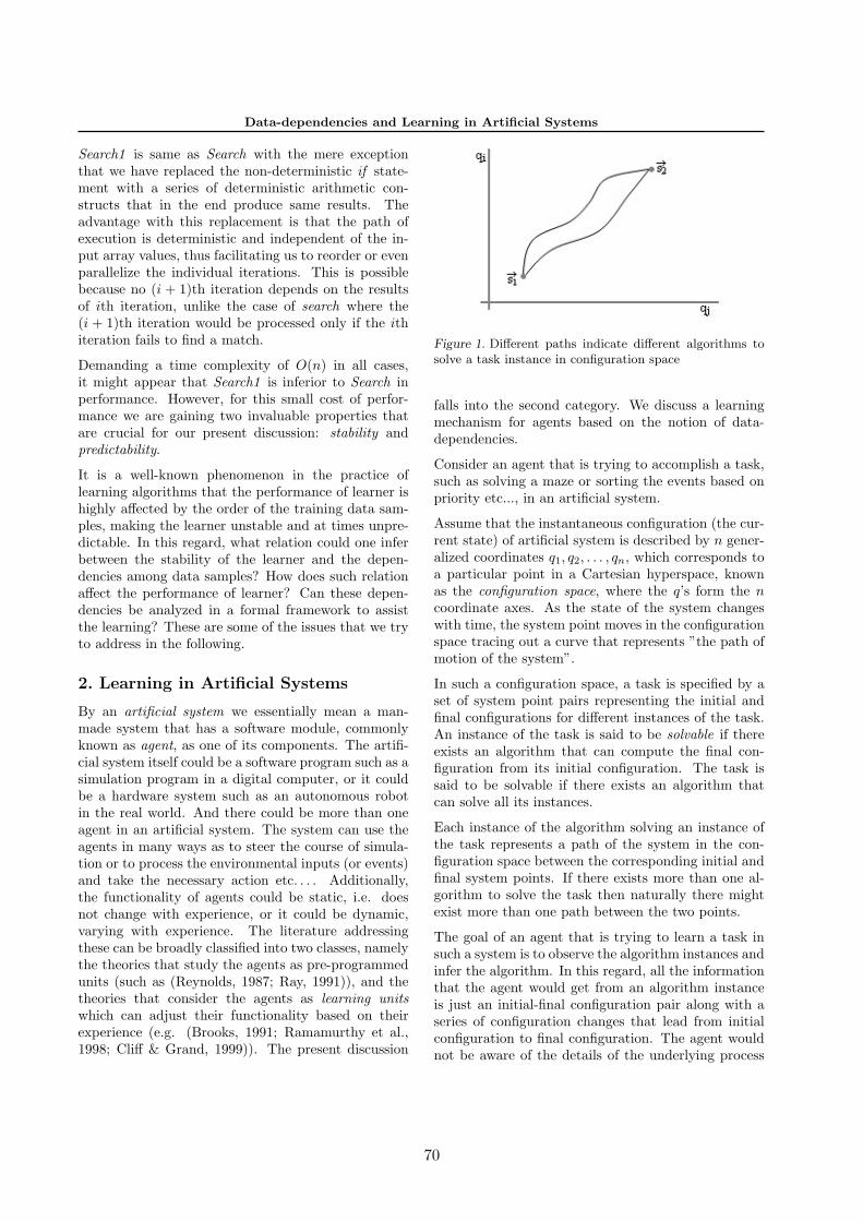
Data-dependencies and Learning in Artificial Systems
Search1 is same as Search with the mere exceptionthat we have replaced the non-deterministic if state-ment with a series of deterministic arithmetic con-structs that in the end produce same results. Theadvantage with this replacement is that the path ofexecution is deterministic and independent of the in-put array values, thus facilitating us to reorder or evenparallelize the individual iterations. This is possiblebecause no (i + 1)th iteration depends on the resultsof ith iteration, unlike the case of search where the(i + 1)th iteration would be processed only if the ithiteration fails to find a match.
Demanding a time complexity of O(n) in all cases,it might appear that Search1 is inferior to Search inperformance. However, for this small cost of perfor-mance we are gaining two invaluable properties thatare crucial for our present discussion: stability andpredictability.
It is a well-known phenomenon in the practice oflearning algorithms that the performance of learner ishighly affected by the order of the training data sam-ples, making the learner unstable and at times unpre-dictable. In this regard, what relation could one inferbetween the stability of the learner and the depen-dencies among data samples? How does such relationaffect the performance of learner? Can these depen-dencies be analyzed in a formal framework to assistthe learning? These are some of the issues that we tryto address in the following.
2. Learning in Artificial Systems
By an artificial system we essentially mean a man-made system that has a software module, commonlyknown as agent, as one of its components. The artifi-cial system itself could be a software program such as asimulation program in a digital computer, or it couldbe a hardware system such as an autonomous robotin the real world. And there could be more than oneagent in an artificial system. The system can use theagents in many ways as to steer the course of simula-tion or to process the environmental inputs (or events)and take the necessary action etc. . . . Additionally,the functionality of agents could be static, i.e. doesnot change with experience, or it could be dynamic,varying with experience. The literature addressingthese can be broadly classified into two classes, namelythe theories that study the agents as pre-programmedunits (such as (Reynolds, 1987; Ray, 1991)), and thetheories that consider the agents as learning unitswhich can adjust their functionality based on theirexperience (e.g. (Brooks, 1991; Ramamurthy et al.,1998; Cliff & Grand, 1999)). The present discussion
Figure 1. Different paths indicate different algorithms tosolve a task instance in configuration space
falls into the second category. We discuss a learningmechanism for agents based on the notion of data-dependencies.
Consider an agent that is trying to accomplish a task,such as solving a maze or sorting the events based onpriority etc..., in an artificial system.
Assume that the instantaneous configuration (the cur-rent state) of artificial system is described by n gener-alized coordinates q1, q2, . . . , qn, which corresponds toa particular point in a Cartesian hyperspace, knownas the configuration space, where the q’s form the ncoordinate axes. As the state of the system changeswith time, the system point moves in the configurationspace tracing out a curve that represents ”the path ofmotion of the system”.
In such a configuration space, a task is specified by aset of system point pairs representing the initial andfinal configurations for different instances of the task.An instance of the task is said to be solvable if thereexists an algorithm that can compute the final con-figuration from its initial configuration. The task issaid to be solvable if there exists an algorithm thatcan solve all its instances.
Each instance of the algorithm solving an instance ofthe task represents a path of the system in the con-figuration space between the corresponding initial andfinal system points. If there exists more than one al-gorithm to solve the task then naturally there mightexist more than one path between the two points.
The goal of an agent that is trying to learn a task insuch a system is to observe the algorithm instances andinfer the algorithm. In this regard, all the informationthat the agent would get from an algorithm instanceis just an initial-final configuration pair along with aseries of configuration changes that lead from initialconfiguration to final configuration. The agent wouldnot be aware of the details of the underlying process
70

Data-dependencies and Learning in Artificial Systems
that is responsible for these changes, and has to inferthe process purely based on the observations.
The agent is said to have ”learned the task” if it canperform the task on its own, by moving the systemfrom any given initial configuration to the correspond-ing final configuration in the configuration space. Itshould be noted that the procedure used (the algo-rithm inferred) by the agent may not be the sameas the original algorithm from whose instances it haslearned.
It should also be noted that the notion of learning thetask, as described above, does not allow any proba-bilistic or approximate solutions. The agent should beable to perform the task correctly under all circum-stances. An additional constraint that we put on theagent is that it should infer the algorithm from as fewalgorithmic instances as possible. This is importantfor agents of both real world systems and simulationsystems alike, for in case of agents observing samplesfrom real world environment it may not be possibleto pickup as many samples as they want, and in caseof simulated environments each sample instance incursan execution cost in terms of time and other resourcesand hence should be traded sparingly.
We formalize these concepts in the following.
2.1. A Formal Framework
Consider an agent that it trying to learn a task T in asystem S whose configuration space is given by
C(S) = ~s1, ~s2, . . . , ~sN,
where each ~si is a system point represented withn−coordinates qi1 , qi2 , . . . , qin
.
Let A be an algorithm to solve the task T, andA1, A2, . . . , Ak be the instances of A solving the in-stances T1, T2, . . . , Tk of T respectively.
In the configuration space each Ti is represented by apair of system points (~si1 , ~si2), and the correspondingAi by a path between those system points.
Let I, F be two operators that when applied to analgorithm instance Ai, yield the corresponding initialand final system points respectively, such as I(Ai) =~si1 and F (Ai) = ~si2 . We also define the correspondingset versions of these operators ~I and ~F as following.For all A′ ⊆ A1, A2, . . . , Ak,
~I(A′) = I(Ai) |Ai ∈ A′,
and~F (A′) = F (Ai) |Ai ∈ A′.
The goal of the agent is to perform T, by mimickingor modeling A, inferring A’s details from a subset ofits instances.
By following the tradition of learning algorithms, letus call A as the target concept, and the subset of its in-stances D = D1, D2, . . . , Dd ⊆ A1, A2, . . . , Ak asthe training set or data samples, and the agent as thelearner. We use the symbol L to denote the learner.
At any instance during the phase of learning the setD can be partitioned into two subsets O,O′ such that
(O ∪O′ = D) ∧ (O ∩O′ = ∅).
The set O ⊆ D denotes the set of data samples thatthe learner has already seen, and the set O′ ⊆ D de-notes the set of data samples the learner has yet to see.Learning progresses by presenting the learner with anunseen sample Di ∈ O′, and marking it as seen, bymoving it to the set O. Starting from O = ∅, O′ = D,this process of transition would be repeated till it be-comes O = D,O′ = ∅.
In this process, each data sample Di decreases the ig-norance of the learner L about the target concept A,and hence could be assigned some specific informa-tion content value that indicates how much additionalinformation L can gain from Di about A.
We can determine the information content values ofdata samples by establishing the concept of a zone,where we treat an ensemble of system points that sharea common relation as a single logical entity.
Definition. A set Z ⊆ C(S) defines a zone if thereexists a function f : C(S) → 0, 1 such that for each~si ∈ C(S) :
f(si) =
1 if ~si ∈ Z,0 if ~si /∈ Z.
The function f is called the characteristic function ofZ.
For the configuration space C(S) = ~s1, ~s2, . . . , ~sm,we can construct an equivalent zone-space Z(S) =Z1, Z2, . . . , Zr, such that the following holds.
∀~si ∃Zi [~si ∈ Zi] ∧ ∀ri=1∀r
j=i+1 [Zi ∩ Zj = ∅] ∧∀r
i=1 [Zi 6= ∅] ∧ ∪ri=1Zi = C(S).
The zone-space can be viewed as a m−dimensionalspace with each Zi being a point in it, where m is somefunction of n whose value depends upon and hencewould be decided by the nature of T. Let the range ofith coordinate of this m−dimensional space be [0, ri].
71

Data-dependencies and Learning in Artificial Systems
If we use the notation |P | to indicate the size of anyset P, then we could represent the volume of the zone-space as
vol(Z(S)) = |Z(S)| =m∏
i=1
ri.
Define an operator ∇ : C(S) → Z(S) that when ap-plied to a system point in the configuration spaceyields the corresponding zone in the zone-space. Sim-ilarly, let ~∇ be the corresponding set version of thisoperator defined as, for all S′ ⊆ C(S),
~∇(S′) = ∇(~si) | ~si ∈ S′.
At any instance the knowledge of L about A dependson the set of samples it has seen till then, and the infor-mation content of a data sample depends on whetherthe sample has already been seen by L or not.
To define formally, the knowledge of the learner, afterhaving seen a set of samples O ⊆ D, is given by
KO(L) =∑
Z∈~∇(~I(O))
|Z| .
The information content of any data sample Di ∈ D,after the learner has seen a set of samples O ⊆ D, isgiven by
ICO(Di) =
|∇(I(Di))| if ∀Dj ∈ O [∇(I(Di)) 6=∇(I(Dj))];
0 otherwise;
and the information content of all data samples wouldbe given by
−→ICO(D) =
∑Z∈~∇(~I(D−O))
|Z| .
It should be noted that the above definitions measurethe information content of data samples relative to thestate of the learner and satisfy the limiting conditionsK∅(L) = 0,
−→ICD(D) = 0.
The process of learning is essentially a process of trans-fer of information from data samples to the learner,resulting in a change in the state of the learner. Whenthese changes are infinitesimal, spanning many steps,the transformation process satisfies the condition thatthe line integral
L =∫ D
∅E do, (2.1)
where E =−→ICO(D)−KO(L), has a stationary value.
This is known as the Hamilton’s principle, which statesthat out of all possible paths by which the learner
could move from K∅(L) to KD(L), it will actuallytravel along that path for which the value of the lineintegral (2.1) is stationary. The phrase ”stationaryvalue” for a line integral typically means that the in-tegral along the given path has same value to withinfirst-order infinitesimals as that along all neighboringpaths (Goldstein, 1980; McCauley, 1997).
We can summarize this by saying that the process oflearning is such that the variation of the line integralL is zero.
δL = δ
∫ D
∅E do = 0.
Thus we can formulate the following conservation the-orem.Theorem 1. The sum KO(L)+
−→ICO(D) is conserved
for all O ⊆ D.
Proof. We shall prove this by establishing thatKOi
(L) +−→ICOi
(D) = KOj(L) +
−→ICOj
(D) for allOi, Oj ⊆ D.
Consider O1, O2 ⊆ D such that |O2| − |O1| = 1. LetO2−O1 = Di. To calculate the information contentvalue of Di, we need to consider two cases.
Case 1. ∇(I(Di)) = ∇(I(Dj)) for some Dj ∈ O1.
In such case, ~∇(~I(O2)) = ~∇(~I(O1)), and henceICO1(Di) = ICO2(Di) = 0.
KO2(L) =∑
Z∈~∇(~I(O2))|Z|
=∑
Z∈~∇(~I(O1))|Z|
= KO1(L).−→ICO2(D) =
−→ICO1(D)− ICO1(D)
=−→ICO1(D).
KO2(L) +−→ICO2(D) = KO1(L) +
−→ICO1(D).
Case 2. ∇(I(Di)) 6= ∇(I(Dj)) for all Dj ∈ O1. Insuch case, ICO1(Di) = |∇(I(Di))| .
−→ICO2(D) =
−→ICO1(D)− ICO1(Di)
=−→ICO1(D)− |∇(I(Di))| .
KO2(L) =∑
Z∈~∇(~I(O2))|Z|
=∑
Z∈~∇(~I(O1+Di)) |Z|
=∑
Z∈~∇(~I(O1))
|Z|+∑
Z∈∇(I(Di))
|Z|
= KO1(L) + |∇(I(Di))| .KO2(L) +
−→ICO2(D) = KO1(L) + |∇(I(Di))|+
−→ICO1(D)− |∇(I(Di))|
= KO1(L) +−→ICO1(D).
72

Data-dependencies and Learning in Artificial Systems
Thus whenever |O2| − |O1| = 1, it holds that
KO2(L) +−→ICO2(D) = KO1(L) +
−→ICO1(D).
Now consider two sets Oi, Oj ⊆ D such that |Oj | −|Oi| = l, l > 1. Let Oj −Oi = Dj1 , . . . , Djl
. We canconstruct sets P1, . . . , Pl−1 such that
P1 = Oi ∪ Dj1, . . . , Pl−1 = Oi ∪ Dj1 , . . . , Djl−1.
Then it holds that
|P1| − |Oi| = |P2| − |P1| = · · · = |Oj | − |Pl−1| = 1.
However, we have proved that
KO2(L) +−→ICO2(D) = KO1(L) +
−→ICO1(D)
whenever |O2| − |O1| = 1, and hence it follows that
KOi(L) +−→ICOi(D) = KP1(L) +
−→ICP1(D),
KP1(L) +−→ICP1(D) = KP2(L) +
−→ICP2(D),
...KPl−1(L) +
−→ICPl−1(D) = KOj
(L) +−→ICOj
(D),
and thereby, KOi(L)+
−→ICOi
(D) = KOj(L)+
−→ICOj
(D).
Hence the sum KO(L) +−→ICO(D) is conserved for all
O ⊆ D.
An important consequence of this theorem is that ir-respective of the order of individual samples that Lchooses to learn from, the gain in its knowledge wouldalways be equal to the corresponding loss in the infor-mation content of the data samples.
KOj (L)−KOi(L) =−→ICOi(D)−
−→ICOj (D).
We now define two metrics – quality and quantity –for the data samples to denote the notions of necessityand sufficiency.
The metric quality measures the relative informationstrength of individual samples, defined as
quality(D) =|D| −
∣∣∣~∇(~I(D))∣∣∣
|D|× 100%.
Ideally a data sample set should have this value to be100%. Smaller values indicate the presence of unnec-essary samples that do not contribute to learning.
Similarly we define the quantity of data samples as
quantity(D) =
∣∣∣~∇(~I(D))∣∣∣
|Z(S)|× 100%.
This is a sufficiency measure and hence a value lessthan 100% indicates the insufficiency of data samplesto complete the learning.
Theorem 2. The knowledge of the learner, aftercompleting the learning over data samples D havingquantity(D) = 100%, would be equal to the volume ofthe configuration space |C(S)| .
Proof. When the quantity(D) = 100%,∣∣∣~∇(~I(D))∣∣∣ = |Z(S)| .
Since ~∇(~I(D)) ⊆ Z(S),∣∣∣~∇(~I(D))∣∣∣ = |Z(S)| ⇒ ~∇(~I(D)) = Z(S).
From theorem 1 we have,
KD(L) +−→ICD(D) = K∅(L) +
−→IC∅(D).
Since K∅(L) = 0 and−→ICD(D) = 0,
KD(L) =−→IC∅(D)
=∑
Z∈~∇(~I(D−∅)) |Z|=
∑Z∈~∇(~I(D)) |Z|
=∑
Z∈Z(S) |Z|= |C(S)| .
Thus when quantity(D) = 100%, KD(L) = |C(S)| .
Theorem 3. The target concept can not be learnt withless than |Z(S)| number of data samples.
Proof. Consider a data sample set D = D1, . . . , Ddhaving quantity(D) = 100% and |D| < |Z(S)| .
Let P = Z(S) − ~∇(~I(D)) = P1, . . . , Pl, l ≥ 1. As-sume that L has learned the target concept completelyfrom D. Then, by theorem 2, KD(L) = |C(S)| , and bytheorem 1,
KD(L) +−→ICD(D) = K∅(L) +
−→IC∅(D).
Since K∅(L) = 0 and−→ICD(D) = 0, it leads to
|C(S)| =−→IC∅(D)
=∑
Z∈~∇(~I(D−∅)) |Z|=
∑Z∈~∇(~I(D)) |Z|
=∑
Z∈(Z(S)−P ) |Z|=
∑Z∈Z(S) |Z| −
∑Z∈P |Z|
= |C(S)| −∑
Z∈P |Z|.
This is not possible unless P = ∅, in which case itwould become Z(S) = ~∇(~I(D)), and |D| ≥ |Z(S)| .Hence proved.
73

Data-dependencies and Learning in Artificial Systems
2.2. A Learning Mechanism Based onData-dependencies
Consider a task instance T1 with end points (~s1, ~s2) inthe configuration space. If we express T1 as a pointfunction f, then we could write ~s2 = f(~s1). An algo-rithm instance A1 that solves T1 would typically im-plement the functionality of f thereby representing apath between ~s1 and ~s2. If there exists more than oneway to implement f, then there exists more than onepath between ~s1 and ~s2. Such a set of paths might bedenoted by f(~s1, α) with f(~s1, 0) representing somearbitrary path chosen to be treated as reference path.
Further, if we select some function η(~x) that vanishesat ~x = ~s1 and ~x = ~s2, then a possible set of variedpaths is given by
f(~x, α) = f(~x, 0) + α η(~x).
It should be noted that all these varied paths terminateat the same end points, that is, f(~x, α) = f(~x, 0) forall values of α.
However, when we try to consider another task in-stance T2 to be represented with these variations, weneed to make them less constrained. The tasks T1 andT2 would not have the same end points in the con-figuration space and hence there would be a variationin the coordinates at those points. We can, however,continue to use the same parameterization as in thecase of single task instance, and represent the familyof possible varied paths by
fi(~x, α) = fi(~x, 0) + α ηi(~x),
where α is an infinitesimal parameter that goes to zerofor some assumed reference path. Here the functionsηi do not necessarily have to vanish at the end points,either for the reference path or for the varied paths.Upon close inspection, one could realize that the varia-tion in these family of paths is composed of two parts.
1. Variations within a task instance due to differentalgorithmic implementations.
2. Variations across task instances due to differentinitial system point configurations.
The learner can overcome the first type of variations byobserving that the end points, and their correspondingzones, are invariant to the paths between them. In thisregard, all the system points that belong to the sameinitial, final zone pair could be learned with a singlealgorithm instance. However, for the second type ofvariations, the learner may not be able to overcomethem without any prior knowledge of the task. All the
Figure 2. Schematic illustration of path variations acrosstask instances in configuration space
different instances of the task would have different cor-responding zones for their end points and hence theyneed to be remembered as they are.
Below we present a mechanism that uses these con-cepts of variations in the configurations paths to infersolutions to the unknown problem instances based onthe solutions to the known problem instances. Thisresults in a learning like behavior where the knownproblem-solution configuration pairs form the trainingset samples. Such samples could be collected by thefollowing procedure.
1. For a given problem identify the appropriate con-figuration space and number of dimensions.
2. Express the solution as a logical relation Rs interms of coordinates of the configuration space.
3. Use Rs to identify an appropriate characteristicfunction Fs to form a solution zone.
4. Use Fs in deciding the characteristic functionsfor other zones and the number of dimensions forzone-space.
5. Define the operator ∇ to map the system pointsfrom configuration space to the zones in zone-space.
6. Define an appropriate variation operator δ in theconfiguration space such that variations in theknown problem configurations would give clue tothe variations in the solution configurations, suchas, solution(x + δx) = solution(x) + δx.
7. Construct the sample problem-solution configura-tion pairs by using any traditional algorithm. The
74

Data-dependencies and Learning in Artificial Systems
samples should be such that all zones are repre-sented.
Once we have all the required data samples with us,the training procedure is simple and straightforward inthat all that is needed is to mark each of the sampleproblem configurations as the reference configurationfor the corresponding zone and remembering the re-spective solution configurations for those references.We can use a memory lookup table to store these ref-erence solutions. The procedure is as follows.
For each data sample Di = (~pi, ~si)
Let Z = ∇(pi);RefProbConfig[Z] = ~pi;RefSolConfig[Z] = ~si;
Once the training is over, we can compute the solutionconfiguration ~s for any given problem configuration ~pin the configuration space as follows.
1. For the given problem configuration ~p, apply theoperator ∇ and find the zone Z = ∇(~p);
2. Get the reference problem configuration ~pi =RefProbConfig[Z], and compute the variationδ(~p, ~pi);
3. Compute the required solution configuration fromthe reference solution configuration by applyingthe variation parameter as:
~s = RefSolConfig[Z] + δ(~p, ~pi);
2.3. An Example Problem
To explain how these concepts of variations in the con-figuration paths could be used in practice, we consideran example problem of sorting. We outline a proce-dure that implements sorting based on the conceptswe have discussed till now.
The reason behind choosing sorting as opposed to anyother alternative is that the problem of sorting hasbeen well studied and well understood, and requires noadditional introduction. However, it should be notedthat our interest here is, rather to explain how zonescan be constructed and used for the sorting problem,than to propose a new sorting algorithm; and hencewe do not consider any performance comparisons. Infact, the procedure we outline below runs with O(n2)time complexity requiring O(2n2
) memory, thus anyperformance comparisons would be futile.
To start with, we can consider the task of sort-ing as being represented by its instances such as(3, 5, 4), (3, 4, 5), where the second element (3, 4, 5)represents the sorted result of first element (3, 5, 4).We can consider these elements as points in a3−dimensional space.
Thus in general given an array of n integers to besorted, we can form a system with n−coordinate axesresulting in an n−dimensional configuration space. Ifwe assume that each element of the array can takea value in the range [0, N ], where N is some maxi-mum integer value, then there would be a total of Nn
system points in the configuration space. That is, fol-lowing our notation from section 2.1, |C(S)| = Nn. Toconstruct the corresponding zone-space for this con-figuration space, consider the following mathematicalspecification for sorting,
∀ni=1∀n
j=1 [ i < j ⇒ a[i] < a[j] ],
where a is an array with n integers. This specifica-tion represents a group of conditions that need to besatisfied by the array if it has to considered as beingin sorted order. Now, we can use this specification inidentifying the following.
1. Number of dimensions of zone-space: The spec-ification involves two quantifiers ∀n
i=1 and ∀nj=1,
with an additional constraint i < j. Thus the validvalues could be i = 1, . . . , n, j = i + 1, . . . , n, re-sulting in a group of n × (n − 1)/2 conditions tobe accounted for. Each condition would form onecoordinate axis in the zone-space and hence wehave n× (n− 1)/2 axes.
2. Range of each axis of zone-space: Since each axisis formed out of the condition (a[i] < a[j]), withvarious values of i, j representing various axes, therange of each axis would be defined by the numberof possible conditions (a[i] < a[j]), (a[i] = a[j])and (a[i] > a[j]), which is three. Hence the rangeof each axis ri = 3.
3. Operator ∇ : Each zone is a point in zone-spacewith n × (n − 1)/2 coordinates. To find thesecoordinate values we need to evaluate n×(n−1)/2conditions (one for each axis) as below.
for(int i=0,r=0; i<n; ++i)for(int j=i+1; j<n; ++j,++r)
ZCoord[r]=((a[i]=a[j])?0:((a[i]<a[j])?1:2));
4. Variation operator δ : We implement the variationoperator using the differences between relative ar-ray positions of numbers before and after sorting.We can use the array indexing and de-indexing
75

Data-dependencies and Learning in Artificial Systems
operations for this purpose. For example, sortinga = 3, 5, 4 produces ~a = 3, 4, 5, which gives usa variation in the indices of elements from (0, 1, 2)to (0, 2, 1). Thus we can use our variation operatorto express ~a as, ~a = a[0], a[2], a[1] .
Once we have these necessary operators with us, wecan start assigning the reference (unsorted, sorted)configuration pairs for each zone by using any tradi-tional sorting algorithm such as heapsort or quicksort,as shown below.
for(int i=0; i < nSamples; ++i)
GetZCoord(Unsorted[i], ZCoord);quicksort(Unsorted[i], Sorted[i]);SetRefConfig(ZCoord, Unsorted[i], Sorted[i]);
It should be noted that we have 3n×(n−1)/2 zones inthe zone-space and hence we need so many sample(unsorted, sorted) pairs as well. However, once wecomplete the training with all those samples, we canuse the following procedure to sort any of the Nn pos-sible arrays.
void LSort(int nArray[], int nSize, int nSorted[])
GetZCoord( nArray, ZCoord );GetRefConfig( ZCoord, RefProb, RefSol);for(int i=0; i < nSize; ++i)
nSorted[i] = nArray[RefSol[i]];
2.4. Limitations
Having presented the mechanism for learning based onthe concepts of variations in the system configurationpaths, here we discuss the limitations of this approach.
Disadvantages: 1. As could be easily understood,the concepts of configuration space and zone-space form the central theme of this ap-proach. However, it may not be always pos-sible to come up with appropriate configura-tion space or zone-space for any given prob-lem. In fact, for many tasks such as facerecognition etc. . . we readily do not have anyclues for logical relations among the data at-tributes. This is one of the biggest limitationsof this approach.
2. To present the learner with some sample con-figurations, we assumed the existence of analgorithm that could solve the task at hand.
However, this assumption may not hold atall times. Once again, face recognition is anexample.
3. The memory requirements are too high. Wehave already seen that we need 3n×(n−1)/2
samples to correctly learn the sorting task.
However, given the goal of mimicking a human beingand the scope of abstract concepts the agents haveto learn from human beings, and given the virtuallyunlimited number of problem instances that could besolved by this learning mechanism, the memory re-quirements should not become a problem at all (notethat the memory requirements do not depend on Nbut on n, so there is no upper limit to the number ofproblem instances that can be solved correctly). Fur-ther advantages are as follows.
Advantages: 1. Independent of the order of train-ing data samples. In this method, the learneris invariant to the order in which it receivesthe data samples. All that a learner does witha data sample is, compute the correspondingzone and mark the sample as a reference forthat zone. This process clearly is indepen-dent of the order of the data samples andhence gives the same results in all circum-stances. It should be noted that the tradi-tional learning algorithms does not guaranteeany such invariance.
2. Additional samples do not create any bias. Ifthere exists more than one sample per zone,the characteristic functions of zones guaran-tee that they all would produce the same re-sults as that of first sample. Hence the train-ing would not be biased by the presence of ad-ditional samples. Further, a sample could berepeated as many times as one wants withoutaffecting the training results. This is usefulfor situations where a robot might be learn-ing from real world, where some typical ob-servations (such as the changing traffic lights,flow of vehicles etc. . . ) would get repeatedmore frequently compared with some rare ob-servations (such as earth quakes or accidentsetc. . . ). Traditional learning algorithms failto provide unbiased results in such situations.
3. Non-probabilistic metrics and accurate re-sults. To meet the demands of artificial sys-tems, the metrics we have devised are com-pletely deterministic and are void of anyprobabilistic assumptions and thus can beadapted to any suitable system.
76

Data-dependencies and Learning in Artificial Systems
4. Expandable to multi-task learning. Thoughwe have concentrated on learning a singletask in this discussion, there is nothing in thismethod that could prevent the learner fromlearning more than one task at the same time.For example, once an agent learns to sortin ascending order (SASC), it can furtherlearn to sort in descending order (SDSC)simply by computing the new variation op-erator δSDSC directly from (δSASC), insteadof from new sample problem-solution config-uration pairs. This saves the training timeand cost for SDSC. However, to implementthis feature the agent should be informed ofthe relation between the tasks a priori. Smartagents that can automatically recognize therelation among tasks based on their configu-ration spaces should be an interesting optionto explore further in this direction.
5. Knowledge transfer. All the knowledge ofthe learner is represented in terms of refer-ence configurations for individual zones. Anylearner who has access to these reference con-figurations can perform equally well as theowner of the knowledge itself, without theneed to go through all the training again.This could lead to the concept of tradableknowledge resources for agents.
6. Perfect partial learning. Just as additionalsamples do not create bias, lack of samplesalso would not create problems for learning.A training set with quantity less than 100%would still give correct results as long as theproblem instance at hand is from one of thelearnt zones. That is, whatever the agentlearns, it learns perfectly. This feature comeshandy to implement low cost bootstrappingrobots with reduced features and functional-ity which can be used as ”data sample sup-pliers” for other full-blown implementaions.This concept of bootstrapping robots is oneof the fundamental concepts of artificial lifestudy in that it might invoke the possibility ofself-replicating robots (Freitas & Gilbreath,1980; Freitas & Merkle, 2004).
3. Conclusions
The notion of data-independence for an algorithmspeaks for constant execution paths across all its in-stances. A variation in execution path is generallyattributable to the variations in the nature of data.When a problem and its solution are viewed as pointsin a system configuration, variations in the problem
configurations can be used to study the variations inthe solution configurations and vice versa. These vari-ations could be used to infer solutions to unknowninstances of problems based on the solutions to theknown instances.
This paper analyzed the problem of data-dependenciesin the learning process and presented a learning mech-anism based on the relations among data attributes.The mechanism constructs a Cartesian hyperspace,namely the configuration space, for any given task, andfinds a set of paths from the initial configuration to fi-nal configuration that represents different instances ofthe task. As part of the learning process the learnergradually gains information from data samples one byone, till all data samples were processed. Once sucha transfer of information is complete, the learner cansolve any instance of the task without any restrictions.
The mechanism presented is independent of the orderof data samples and has the flexibility to be expand-able to multi-task learning. However, the practical-ity of this approach may be hindered by the lack ofappropriate algorithms that could provide sample in-stances. Further study to eliminate such bottleneckscould make this a perfect choice to implement learningbehavior in artificial agents.
References
Angluin, D. (1992). Computational learning theory:survey and selected bibliography. Proceedings of thetwenty-fourth annual ACM symposium on Theory ofcomputing (pp. 351–369). New York: ACM Press.
Balmer, M., Cetin, N., Nagel, K., & Raney, B. (2004).Towards truly agent-based traffic and mobility simu-lations. AAMAS ’04: Proceedings of the Third Inter-national Joint Conference on Autonomous Agentsand Multiagent Systems (pp. 60–67). Washington,DC, USA: IEEE Computer Society.
Brooks, R. A. (1991). Intelligence without reason. Pro-ceedings of the 12th International Joint Conferenceon Artificial Intelligence (IJCAI-91) (pp. 569–595).San Mateo, CA, USA: Morgan Kaufmann publishersInc.
Brugali, D., & Sycara, K. (2000). Towards agentoriented application frameworks. ACM ComputingSurveys, 32, 21–27.
Bryson, J. J. (2003). Action selection and individua-tion in agent based modelling. Proceedings of Agent2003: Challenges of Social Simulation.
77

Data-dependencies and Learning in Artificial Systems
Cliff, D., & Grand, S. (1999). The creatures globaldigital ecosystem. Artificial Life, 5, 77–93.
Collins, J. C. (2001). On the compatibility betweenphysics and intelligent organisms (Technical ReportDESY 01-013). Deutsches Elektronen-SynchrotronDESY, Hamburg.
Decugis, V., & Ferber, J. (1998). Action selection inan autonomous agent with a hierarchical distributedreactive planning architecture. AGENTS ’98: Pro-ceedings of the second international conference onAutonomous agents (pp. 354–361). New York, NY,USA: ACM Press.
Franklin, S. (2005). A ”consciousness” based architec-ture for a functioning mind. In D. N. Davis (Ed.),Visions of mind, chapter 8. IDEA Group INC.
Freitas, R. A., & Gilbreath, W. P. (Eds.). (1980).Advanced automation for space missions, Proceed-ings of the 1980 NASA/ASEE Summer Study. Na-tional Aeronautics and Space Administration andthe American Society for Engineering Education.Santa Clara, California: NASA Conference Publi-cation 2255.
Freitas, R. A., & Merkle, R. C. (2004). Kinematicself-replicating machines. Georgetown, TX: LandesBioscience.
Goldstein, H. (1980). Classical mechanics. Addison-Wesley Series in Physics. London: Addision-Wesley.
Kamareddine, F., Monin, F., & Ayala-Rincon, M.(2002). On automating the extraction of programsfrom proofs using product types. Electronic Notesin Theoretical Computer Science, 67, 1–21.
Katsuhiko, T., Takahiro, K., & Yasuyoshi, I. (2002).Translating multi-agent autoepistemic logic intologic program. Electronic Notes in Theoretical Com-puter Science, 70, 1–18.
Kearns, M. J. (1990). The computational complexity ofmachine learning. ACM Distinguished Dissertation.Massachusetts: MIT Press.
Lau, T., Domingos, P., & Weld, D. S. (2003). Learn-ing programs from traces using version space alge-bra. K-CAP ’03: Proceedings of the internationalconference on Knowledge capture (pp. 36–43). NewYork, USA: ACM Press.
Laue, T., & Rofer, T. (2004). A behavior architecturefor autonomous mobile robots based on potentialfields. RoboCup 2004. Springer-Verlag.
Littlestone, N. (1987). Learning quickly when irrele-vant attributes abound: A new linear-threshold al-gorithm. Machine Learning, 2.
Lopez, R., & Armengol, E. (1998). Machine learningfrom examples: Inductive and lazy methods. Data& Knowledge Engineering, 25, 99–123.
Maes, P. (1989). How to do the right thing. ConnectionScience Journal, 1.
McCauley, J. (1997). Classical mechanics. CambridgeUniversity Press.
Moses, Y. (1992). Knowledge and communication: Atutorial. TARK ’92: Proceedings of the 4th con-ference on Theoretical aspects of reasoning aboutknowledge (pp. 1–14). San Francisco, CA, USA:Morgan Kaufmann Publishers Inc.
Raedt, L. D. (1997). Logical settings for concept-learning. Artificial Intelligence, 95, 187–201.
Ramamurthy, U., Franklin, S., & Negatu, A. (1998).Learning concepts in software agents. From Ani-mals to Animats 5: Proceedings of The Fifth Inter-national Conference on Simulation of Adaptive Be-havior. Cambridge: MIT Press.
Ray, T. S. (1991). Artificial life ii, chapter An Ap-proach to the Synthesis of Life. Newyork: Addison-Wesley.
Ray, T. S. (1994). Evolution, complexity, entropy andartificial reality. Physica D, 75, 239–263.
Reynolds, C. W. (1987). Flocks, herds, and schools: Adistributed behavioral model. Computer Graphics,21, 25–34.
Schmidhuber, J. (2000). Algorithmic theories of every-thing (Technical Report IDSIA-20-00 (Version 2.0)).Istituto Dalle Molle di Studi sull’Intelligenza Artifi-ciale, Manno-Lugano, Switzerland.
Wilson, S. W. (1994). Zcs: a zeroth level classifiersystem. Evolutionary Computation, 2, 1–18.
Zurek, W. H. (1989). Algorithmic randomness andphysical entropy. Physical Review A, 40, 4731–4751.
78


Author Index
Aguilar, Ramiro 59Alonso, Luis 59De Raedt, L. 37Frasconi, P. 37GopalaKrishna, Palem 69Kitzelmann, Emanuel 15Lopez, Vivian 59Monakhova, Emilia 29Monakhov, Oleg 29Moreno, Marıa N. 59Muggleton, Stephen 9Passerini, A. 37Rao, M. R. K. Krishna 51Schmidhuber, Jurgen 11Schmid, Ute 15Wysotzki, Fritz 13
81