wright-fisher processesdb5d/summerschool09/lectures-dd/lectures6-7.pdf · wright-fisher markov...

Chapter 5

Wright-Fisher Processes

Figure 5.1: Fisher and Wright

5.1 Introductory remarks

The BGW processes and birth and death processes we have studied in the previouschapters have the property that

(5.1) Xn → 0 or ∞, a.s.

A more realistic model is one in which the population grows at low populationdensities and tends to a steady state near some constant value. The Wright-Fisher model that we consider in this chapter (and the corresponding Morancontinuous time model) assume that the total population remains at a constantlevel N and focusses on the changes in the relative proportions of the differenttypes. Fluctuations of the total population, provided that they do not becometoo small, result in time-varying resampling rates in the Wright-Fisher model butdo not change the main qualitative features of the conclusions.

The branching model and the Wright-Fisher idealized models are complemen-tary. The branching process model provides an important approximation in twocases:

69

70 CHAPTER 5. WRIGHT-FISHER PROCESSES

• If the total population density becomes small then the critical and nearcritical branching process provides an useful approximation to compute ex-tinction probabilities.

• If a new type emerges which has a competitive advantage, then the super-critical branching model provides a good approximation to the growth ofthis type as long as its contribution to the total population is small.

Models which incorporate multiple types, supercritical growth at low densitiesand have non-trivial steady states will be discussed in a later chapter. Theadvantage of the idealized models we discuss here is the possibility of explicitsolutions.

5.2 Wright-Fisher Markov Chain Model

The classical neutral Wright-Fisher (1931) model is a discrete time model of apopulation with constant size N and types E = 1, 2. Let Xn be the numberof type 1 individuals at time n. Then Xn is a Markov chain with state space0, . . . , N and transition probabilities:

P (Xn+1 = j|Xn = i) =

(Nj

)(i

N

)j (1− i

N

)N−j, j = 0, . . . , N.

In other words at generation n+ 1 this involves binomial sampling with prob-ability p = Xn

N, that is, the current empirical probability of type 1. Looking

backwards from the viewpoint of generation n+ 1 this can be interpreted as hav-ing each of the N individuals of the (n + 1)st generation “pick their parents atrandom” from the population at time n.

Similarly, the neutralK-allele Wright Fisher model with typesEK = e1, . . . , eKis given by a Markov chain Xn with state space \(EK) (counting measures) and

P (Xn+1 = (β1, . . . βK)|Xn = (α1, . . . , αK))(5.2)

=N !

β1!β2! . . . βK !

(α1

N

)β1

. . .(αKN

)βKIn this case the binomial sampling is simply replaced by multinomial sampling.

Consider the multinomial distribution with parameters (N, p1, . . . , pK). Thenthe moment generating function is given by

(5.3) M(θ1, . . . , θK) = E(exp(K∑i=1

θiXi)) =

(K∑i=1

pieθi

)N

Then

(5.4) E(Xi) = Npi, Var(Xi) = Npi(1− pi),

5.2. WRIGHT-FISHER MARKOV CHAIN MODEL 71

and

(5.5) Cov(Xi,Xj) = −Npipj, i 6= j.

Remark 5.1 We can relax the assumptions of the Wright-Fisher model in twoways. First, if we relax the assumption of the total population constant, equal toN , we obtain a Fisher-Wright model with variable resampling rate (e.g. Donnellyand Kurtz [167] and Kaj and Krone [359]).

To introduce the second way to relax the assumptions note that we can obtainthe Wright-Fisher model as follows. Consider a population of N individuals ingeneration n with possible types in EK, Y n

1 , . . . , YnN . Assume each individual has

a Poisson number of offspring with mean m, (Z1, . . . , ZN) and the offspring is ofthe same type as the parent. Then

conditioned onN∑i=1

Zi = N,

the resulting population (Y(n+1)

1 , . . . , Y(n+1)N ) is multinomial (N ; 1

N; . . . , 1

N), that

is, we have a a multitype (Poisson) branching process conditioned to have constanttotal population N . If we then define

(5.6) pn+1(i) =1

N

N∑j=1

1(Y(n+1)j = i), i = 1, . . . , K,

then (pn+1(1), . . . , pn+1(K)) is multinomial (N ; pn(1), . . . , pn(K)) where

(5.7) pn(i) =1

N

N∑j=1

1(Y nj = i), i = 1, . . . , K.

We can generalize this by assuming that the offspring distribution of the individ-uals is given by a common distribution on N0. Then again conditioned the totalpopulation to have constant size N the vector (Y n+1

1 , . . . , Y n+1N ) is exchangeable

but not necessarily multinomial. This exchangeability assumption is the basis ofthe Cannings Model (see e.g. Ewens [243]).

A basic phenomenon of neutral Wright-Fisher without mutation is fixation,that is, the elimination of all but one type at a finite random time. To see thisnote that for each j = 1, . . . , K, δj ∈ P(EK) are absorbing states and Xn(j) isa martingale. Therefore Xn → X∞, a.s. Since Var(Xn+1) = NXn(1 − Xn), thismeans that X∞ = 0 or 1, a.s. and Xn must be 0 or 1 after a finite number ofgenerations (since only the values k

Nare possible).


5.2.1 Types in population genetics

The notion of type in population biology is based on the genotype. The genotypeof an individual is specified by the genome and this codes genetic informationthat passes, possibly modified, from parent to offspring (parents in sexual re-production). The genome consists of a set of chromosomes (23 in humans). Achromosome is a single molecule of DNA that contains many genes, regulatoryelements and other nucleotide sequences. A given position on a chromosome iscalled a locus (loci) and may be occupied by one or more genes. Genes code forthe production of a protein. The different variations of the gene at a particularlocus are called alleles. The ordered list of loci for a particular genome is calleda genetic map. The phenotype of an organism describes its structure and be-haviour, that is, how it interacts with it environment. The relationship betweengenotype and phenotype is not necessarily 1-1. The field of epigenetics studiesthis relationship and in particular the mechanisms during cellular developmentthat produce different outcomes from the same genetic information.

Diploid individuals have two homologous copies of each chromosome, usuallyone from the mother and one from the father in the case of sexual reproduction.Homologous chromosomes contain the same genes at the same loci but possiblydifferent alleles at those genes.

5.2.2 Finite population resampling in a diploid population

For a diploid population with K-alleles e1, . . . , eK at a particular gene we can

focus on the set of types given by E2K where K(K+1)

2is the set of unordered pairs

(ei, ej). The genotype (ei, ej) is said to be homozygous (at the locus in question)if ei = ej, otherwise heterozygous.

Consider a finite population of N individuals. Let

Pij = proportion of type (ei, ej)

Then, pi, the proportion of allele ei is

pi = Pii +1

2

∑j 6=i

Pij.

The probability Pij on E2K is said to be a Hardy-Weinberg equilibrium if

(5.8) Pij = (2− δij)pipj.

This is what is obtained if one picks independently the parent types ei and ejfrom a population having proportions pi ( in the case of sexual reproductionthis corresponds to “random mating”).

Consider a diploid Wright-Fisher model of with N individuals therefore 2Ngenes with random mating. This means that an individual at generation (n+ 1)has two genes randomly chosen from the 2N genes in generation n.

5.2. WRIGHT-FISHER MARKOV CHAIN MODEL 73

In order to introduce the notions of identity by descent and genealogy we as-sume that in generation 0 each of the 2N genes correspond to different alleles.Now consider generation n. What is the probability, Fn, that an individual ishomozygous, that is, two genes selected at random are of the same type (ho-mozygous)? This will occur only if they are both descendants of the same genein generation 0.

First note that in generation 1, this means that an individual is homozygousonly if the same allele must be selected twice and this has probability 1

2N. In

generation n + 1 this happens if the same gene is selected twice or if differentgenes are selected from generation n but they are identical alleles. Therefore,

(5.9) F1 =1

2N, Fn =

1

2N+ (1− 1

2N)Fn−1.

Let Hn := 1− Fn (heterozygous). Then

(5.10) H1 = 1− 1

2N, Hn = (1− 1

2N)Hn−1, Hn = (1− 1

2N)n

Two randomly selected genes are said to be identical by descent if they are thesame allele. This will happen if they have a common ancestor. Therefore if T2,1

denotes the time in generations back to the common ancestor we have

(5.11) P (T2,1 > n) = Hn = (1− 1

2N)n, n = 0, 1, 2, . . . ,

(5.12) P (T2,1 = n) =1

2N(1− 1

2N)n−1, n = 1, 2 . . . .

Similarly, for k randomly selected genes they are identical by descent if theyall have a common ancestor. We can consider the time Tk,1 in generations backto the most recent common ancestor of k individuals randomly sampled fromthe population. We will return to discuss the distribution of Tk,1 in the limit asN →∞ in Chapter 9.

5.2.3 Diploid population with mutation and selection

In the previous section we considered only the mechanism of resampling (geneticdrift). In addition to genetic drift the basic genetic mechanisms include mutation,selection and recombination. In this subsection we consider the Wright-Fishermodel incorporating mutation and selection.

For a diploid population of size N with mutation, selection and resampling thereproduction cycle can be modelled as follows (cf [225], Chap. 10). We assumethat in generation 0 individuals have genotypic proportions Pij and thereforethe proportion of type i (in the population of 2N genes) is

pi = Pii +1

2

∑j 6=i

Pij.


Stage I:In the first stage diploid cells undergo meiotic division producing haploid gametes(single chromosomes), that is, meiosis reduces the number of sets of chromosomesfrom two to one. The resulting gametes are haploid cells; that is, they contain onehalf a complete set of chromosomes. When two gametes fuse (in animals typicallyinvolving a sperm and an egg), they form a zygote that has two complete sets ofchromosomes and therefore is diploid. The zygote receives one set of chromosomesfrom each of the two gametes through the fusion of the two gametes. By theassumption of random mating, then in generation 1 this produces zygotes inHardy-Weinberg proportions (2− δij)pipj.

Stage II: Selection and Mutation.Selection. The resulting zygotes can have different viabilities for survival. The

viability of (ei, ej) has viability Vij. The the proportions of surviving zygotes areproportional to the product of the viabilities and the Hardy-Weinberg propor-tions, that is,

(5.13) P selk,` =

Vk` · (2− δk`)pkp`∑k′≤`′(2− δk′`′)Vk′`′pk′p`′

Mutation. We assume that each of the 2 gametes forming zygote can (inde-pendently) mutate with probability pm and that if a gamete of type ei mutatesthen it produces a gamete of type ej with probability mij.

(5.14)

P sel,mutij = (1− 1

2δij)

∑k≤`

(mkim`j +mkjm`i)Pselk`

= (1− 1

2δij)

∑k≤`

(mkim`j +mkjm`i)Vk` · (2− δk`)pkp`∑

k′≤`′(2− δk′`′)Vk′`′pk′p`′

Stage III: Resampling. Finally random sampling reduces the population to Nadults with proportions P next

ij where

(5.15) (P nextij )i≤j ∼

1

Nmultinomial (N, (P sel,mut

ij )i≤j).

We then obtain a population of 2N gametes with proportions

(5.16) pnexti = P next

ii +1

2

∑j 6=i

P nextij .

Therefore we have defined the process XNn n∈N with state space PN (EK). If

XNn is a Markov chain we defined the transition function

P (XNn+1 = (pnext

1 , . . . , pnextK )|XN

n = (p1, . . . , pK)) = πp1,...,pK(pnext

1 , . . . , pnextK )

5.3. DIFFUSION APPROXIMATION OF WRIGHT-FISHER 75

where the function π is obtained from (5.14), (5.15), (5.16). See Remark 5.7.

5.3 Diffusion Approximation of Wright-Fisher

5.3.1 Neutral 2-allele Wright-Fisher model

As a warm-up to the use of diffusion approximations we consider the case of 2alleles A1, A2, (k = 2). Let XN

n denote the number of individuals of type A1 atthe nth generation. Then as above XN

n n∈N is a Markov chain.

Theorem 5.2 (Neutral case without mutation) Assume that N−1XN0 → p0 as

N →∞. Then

pN(t) : t ≥ 0 ≡ N−1XNbNtc, t ≥ 0 =⇒ p(t) : t ≥ 0

where p(t) : t ≥ 0 is a Markov diffusion process with state space [0, 1] and withgenerator

(5.17) Gf(p) =1

2p(1− p) d

2

dp2f(p)

if f ∈ C2([0, 1]). This is equivalent to the pathwise unique solution of the SDE

dp(t) =√p(t)(1− p(t))dB(t)

p(0) = p0.

Proof. Note that in this case XNn+1 is Binomial(N, pn) where pn = XN

n

N. Then

from the Binomial formula,

EXNn

(XNn+1

N) =

XNn

N

EXNn

[

(XNn+1

N− XN

n

N

)2

| XNn

N] =

1

N

(XNn

N

(1− XN

n

N

)).

We can then verify that

(5.18) pN(t) := N−1XNbNtc : t ≥ 0 is a martingale

with

E(pN(t2)− pN(t1))2 = E

bNt2c∑k=bNt1c

(pN(k + 1

N)− pN(

k

N))2(5.19)

=1

NE

bNt2c∑k=bNt1c

pN(k

N)(1− pN(

k

N))


and then that

(5.20) MN(t) = p2N(t)− 1

N

bNt2c∑k=bNt1c

pN(k

N)(1− pN(

k

N))

is a martingale.Let PN

pN∈ P(D[0,1]([0,∞)) denote the probability law of pN(t)t≥0 with

pN(0) = pN . From this we can prove that the sequence PNpN (0)N∈N is tight

on P(D[0,∞)([0, 1])). To verify this as in the previous chapter we use Aldous cri-terion PN

pN (0)(pN(τN + δN)− pN(τN) > ε)→ 0 as N →∞ for any stopping times

τN ≤ T and δN ↓ 0. This follows easily from the strong Markov property, (5.19)and Chebyshev’s inequality. Since the processes pN(·) are bounded it then followsthat for any limit point Pp0 of PN

pN (0) we have

(5.21)

p(t)t≥0 is a bounded martingale with p(0) = p0 and with increasing process

〈p〉t =

∫ t

0

p(s)(1− p(s))ds.

Since the largest jump of pN(·) goes to 0 as N → ∞ the limiting process iscontinuous (see Theorem 17.14 in the Appendix). Also, by the Burkholder-Davis-Gundy inequality we have

(5.22) E((p(t2)− p(t1))4) ≤ const · (t2 − t1)2,

so that p(t) satisfies Kolmogorov’s criterion for a.s. continuous.We can then prove that there is a unique solution to this martingale problem,

that is, for each p there exists a unique probability measure on C[0,∞)([0,∞)) sat-isfying (5.21) and therefore this defines a Markov diffusion process with generator(5.17).

The uniqueness can proved by determining all joint moments of the form

(5.23) Ep((p(t1)k1 . . . (p(t`))k`), 0 ≤ t1 < t2 < · · · < t`, ki ∈ N

by solving a closed system of differential equation. It can also be proved usingduality and this will be done in detail below (Chapter 7) in a more general case.)

We now give an illustrative application of the diffusion approximation, namelythe calculation of expected fixation times.

Corollary 5.3 (Expected fixation time.) Let τ := inft : p(t) ∈ 0, 1 denotethe fixation time of the diffusion process. Then

Ep[τ ] = f(p) = −[p log p+ (1− p) log(1− p)].


Proof. Let f ∈ C2([0, 1]), f(0) = f(1) = 0. Let g(p) :=∫∞

0Tsf(p)ds, and

note that as f ↑ 1(0,1) this converges to the expected time spent in (0, 1). Sincep(t)→ 0, 1 as t→∞, a.s., we can show that

G

(∫ t

0

Tsf(p)ds

)=

∫ t

0

GTsf(p)ds = Ttf(p)− f(p)→ 0− f(p) as t→∞,

that is,

Gg(p) = −f(p)

where G is given by (5.17).Applying this to a sequence of C2 functions increasing to 1(0,1) we get

Ep(τ) =

∫ ∞0

Pp(τ > t)dt

=

∫ ∞0

Tt1(0,1)(p)dt

= g(p)

We then obtain g(p) by solving the differential equation Gg(p) = −1 with bound-ary conditions g(0) = g(1) = 0 to obtain

Ep[τ ] = g(p) = −[p log p+ (1− p) log(1− p)].

Let τN denote the fixation time for N−1X[Nt]. We want to show that

(5.24) EXN0N

[τN ]→ Ep0 [τ ] ifXN

0

N→ p and N →∞.

However note that τ is not a continuous function on D([0,∞), [0, 1]). The weakconvergence can be proved for τ ε = inft : p(t) 6∈ (ε, 1− ε) (because there is no“slowing down” here). To complete the proof it can be verified that for δ > 0

(5.25) limε→0

lim supN→∞

P (|τ εN − τN | > δ) = 0

(see Ethier and Kurtz, [225], Chapt. 10, Theorem 2.4).

2-allele Wright-Fisher with mutation

For each N consider a Fisher-Wright population of size MN and with mutationrates m12 = u

NA1 → A2 and m21 = v

NA2 → A1.

In this case XNn+1 is Binomial(MN , pn) with

(5.26) pn = (1− u

N)XNn

MN

+v

N(1− XN

n

MN

).


We now consider

(5.27) pN(t) =1

MN

XbNtc.

If we assume that

(5.28) γ = limN→∞

N

MN

,

then the diffusion approximation is given by the diffusion process pt with gener-ator

(5.29) Gf(p) =γ

2p(1− p) ∂

2

∂p2+ [−up+ v(1− p)] ∂

∂p.

In this case the domain of the generator involves boundary conditions at 0 and1 (see [225], Chap. 8, Theorem 1.1) but we will not need this.

Remark 5.4 Note that the diffusion coefficient is proportional to the inverse pop-ulation size. Below for more complex models we frequently think of the diffusioncoefficient in terms of inverse effective population size.

Error estimates

Consider a haploid Wright-Fisher population of size M with mutation rates m12 =u, m21 = v.

Let p(M,u,v)t denote the diffusion process with generator (5.29) with γ = 1

M.

Then if α, β ≥ 0, the law of

(5.30) Z(α,β)t t≥0 := p

(M, αM, βM

)t

is independent of M and is a Wright-Fisher diffusion with generator

(5.31) Gf(p) =γ

2p(1− p) ∂

2

∂p2+ [−αp+ β(1− p)] ∂

∂p.

The assumption of mutation rates of order O( 1N

) corresponds to the case inwhich both mutation and genetic drift are of the same order and appear in thelimit as population sizes goes to ∞. Other only one of the two mechanismsappears in the limit as N →∞.

On the other hand one can consider the diffusion process as an approximationto the finite population model. Ethier and Norman ([228]) obtained an estimateof the error due to the diffusion approximation in the calculation of the expectedvalue of a smooth function of the nth generation allelic frequency.


To formulate their result consider the Wright-Fisher Markov chain model

XM,u,v)n with population size M and one-step mutation probabilities m12 =

u, m21 = v and p(M,u,v)t the Wright-Fisher diffusion with generator (5.29) with

γ = 1M

.

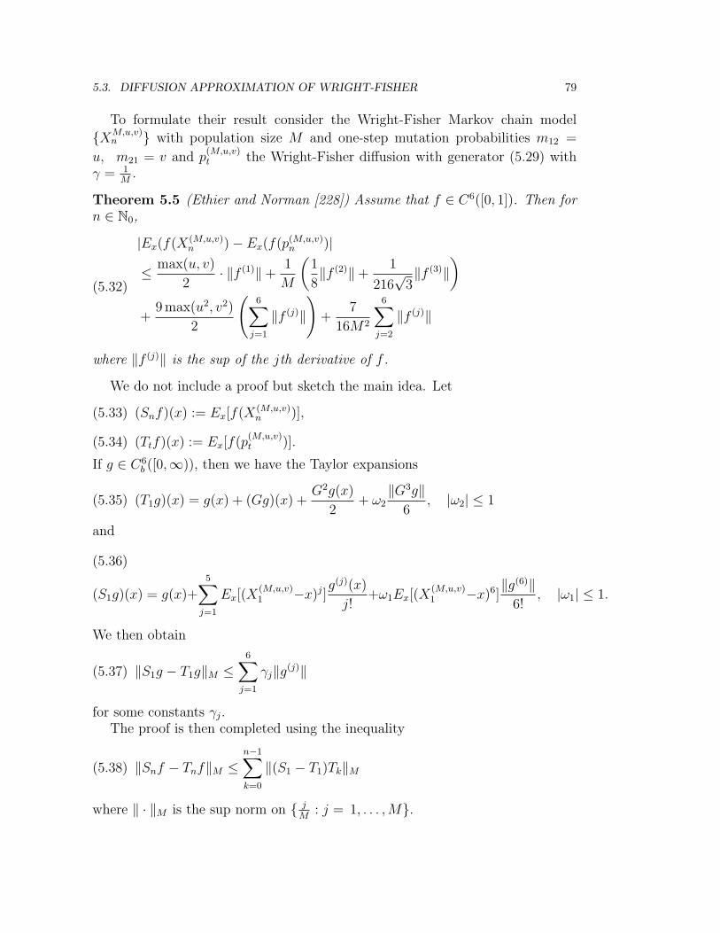
Theorem 5.5 (Ethier and Norman [228]) Assume that f ∈ C6([0, 1]). Then forn ∈ N0,

(5.32)

|Ex(f(X(M,u,v)n )− Ex(f(p(M,u,v)

n )|

≤ max(u, v)

2· ‖f (1)‖+

1

M

(1

8‖f (2)‖+

1

216√

3‖f (3)‖

)+

9 max(u2, v2)

2

(6∑j=1

‖f (j)‖

)+

7

16M2

6∑j=2

‖f (j)‖

where ‖f (j)‖ is the sup of the jth derivative of f .

We do not include a proof but sketch the main idea. Let

(5.33) (Snf)(x) := Ex[f(X(M,u,v)n )],

(5.34) (Ttf)(x) := Ex[f(p(M,u,v)t )].

If g ∈ C6b ([0,∞)), then we have the Taylor expansions

(5.35) (T1g)(x) = g(x) + (Gg)(x) +G2g(x)

2+ ω2

‖G3g‖6

, |ω2| ≤ 1

and

(5.36)

(S1g)(x) = g(x)+5∑j=1

Ex[(X(M,u,v)1 −x)j]

g(j)(x)

j!+ω1Ex[(X

(M,u,v)1 −x)6]

‖g(6)‖6!

, |ω1| ≤ 1.

We then obtain

(5.37) ‖S1g − T1g‖M ≤6∑j=1

γj‖g(j)‖

for some constants γj.The proof is then completed using the inequality

(5.38) ‖Snf − Tnf‖M ≤n−1∑k=0

‖(S1 − T1)Tk‖M

where ‖ · ‖M is the sup norm on jM

: j = 1, . . . ,M.


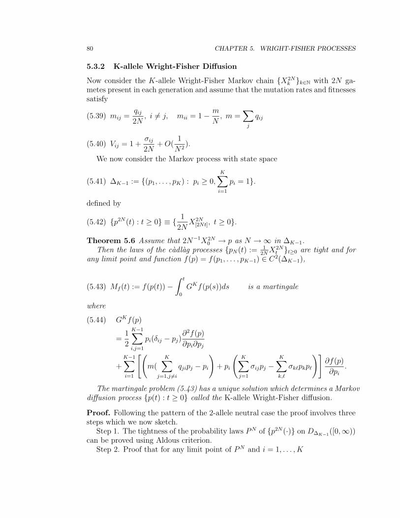
5.3.2 K-allele Wright-Fisher Diffusion

Now consider the K-allele Wright-Fisher Markov chain X2Nk k∈N with 2N ga-

metes present in each generation and assume that the mutation rates and fitnessessatisfy

(5.39) mij =qij2N

, i 6= j, mii = 1− m

N, m =

∑j

qij

(5.40) Vij = 1 +σij2N

+O(1

N2).

We now consider the Markov process with state space

(5.41) ∆K−1 := (p1, . . . , pK) : pi ≥ 0,K∑i=1

pi = 1.

defined by

(5.42) p2N(t) : t ≥ 0 ≡ 1

2NX2N

[2Nt], t ≥ 0.

Theorem 5.6 Assume that 2N−1X2N0 → p as N →∞ in ∆K−1.

Then the laws of the cadlag processes pN(t) := 12NX2Nt t≥0 are tight and for

any limit point and function f(p) = f(p1, . . . , pK−1) ∈ C2(∆K−1),

(5.43) Mf (t) := f(p(t))−∫ t

0

GKf(p(s))ds is a martingale

where

GKf(p)(5.44)

=1

2

K−1∑i,j=1

pi(δij − pj)∂2f(p)

∂pi∂pj

+K−1∑i=1

[(m(

K∑j=1,j 6=i

qjipj − pi

)+ pi

(K∑j=1

σijpj −K∑k,`

σk`pkp`

)]∂f(p)

∂pi.

The martingale problem (5.43) has a unique solution which determines a Markovdiffusion process p(t) : t ≥ 0 called the K-allele Wright-Fisher diffusion.

Proof. Following the pattern of the 2-allele neutral case the proof involves threesteps which we now sketch.

Step 1. The tightness of the probability laws PN of p2N(·) on D∆K−1([0,∞))

can be proved using Aldous criterion.Step 2. Proof that for any limit point of PN and i = 1, . . . , K


Mi(t) := pi(t)− pi(0)−∫ t

0

[m

(K∑j=1

qjipj(s)− pi(s)

)(5.45)

+pi(s)

(K∑j=1

σijpj(s)−K∑k,`

σk`pk(s)p`(s)

) ]ds

is a martingale with quadratic covariation process

(5.46) 〈Mi,Mj〉t =1

2

∫ t

0

pj(s)(δij − pi(s))ds

To verify this, let F k2N

= σp2Ni ( `

2N) : ` ≤ k, i = 1, . . . , K. Then we have for

k ∈ N

(5.47)

E[p2Ni (

k + 1

2N)− p2N

i (k

2N) | F k

2N]

=1

2N

[m

(K∑

j=1,j 6=i

qjimp2Nj (

k

2N)− p2N

i (k

2N)

)

+

(K∑j=1

σijp2Nj (

k

2N)−

K∑k,`=1

σk`p2Nk (

k

2N)p2N` (

k

2N)

)]

+ o(1

2N)

(5.48) Cov(p2Ni (

k + 1

2N), p2N

j (k + 1

2N)|F k

2N) =

p2Ni

2N(k

2N)(δij − p2N

j (k

2N)) + o(

1

N)

Remark 5.7 The Markov property for XNn follows if in the resampling step the

P sel,mutij are in Hardy-Weinberg proportions which implies that the pnext

i are

(5.49) multinomial(2N, (psel,mut1 , . . . , psel,mut

K )).

This is true without selection or with multiplicative selection Vij = ViVj (whichleads to haploid selection in the diffusion limit) but not in general. In the diffusionlimit this can sometimes be dealt with by the O( 1

N2 ) term in (5.40). In generalthe diffusion limit result remains true but the argument is more subtle. The ideais that the selection-mutation changes the allele frequencies more slowly thanthe mechanism of Stages I and III which rapidly bring the frequencies to Hardy-Weinberg equilibrium - see [225], Chap. 10, section 3.


Then for each N and i

M2Ni (t) := p2N

i (t)− p2Ni (0)−

∫ t

0

[m

(K∑

j=1,j 6=i

qjip2Nj (s)− p2N

i (s)

)(5.50)

+p2Ni (s)

(K∑j=1

σijp2Nj (s)−

K∑k,`

σk`p2Nk (s)p2N

` (s)

) ]dsN + o(

1

N)

is a martingale and for i, j = 1, . . . , K

E[(M2Ni (t2)−M2N

i (t1))(M2Nj (t2)−M2N

j (t1))](5.51)

=1

2NE

b2Nt2c∑k=b2Nt1c

p2Ni (

k

2N)(δij − p2N

j (k

2N)) + o(

1

N).

Step 3. Proof that there exists a unique probability measure on C∆K−1([0,∞))

such that (5.45) and (5.46) are satisfied.Uniqueness can be proved in the neutral case, σ ≡ 0, by showing that moments

are obtained as unique solutions of a closed system of differential equations.

Remark 5.8 The uniqueness when σ is not zero follows from the dual represen-tation developed in the next chapter.

5.4 Stationary measures

A special case of a theorem in Section 8.3 implies that if the matrix (qij) isirreducible, then the Wright-Fisher diffusion is ergodic with unique stationarydistribution.

5.4.1 The Invariant Measure for the neutral K-alleles WF Diffusion

Consider the neutral K-type Wright-Fisher diffusion with type-independent mu-tation (Kingman’s “house-of-cards” mutation model) with generator

GKf(p) =1

2

K−1∑i,j=1

pi(δij − pj)∂2f(p)

∂pi∂pj+θ

2

K−1∑i=1

(νi − pi)∂f(p)

∂pi.

where the type-independent mutation kernel is given by ν ∈ ∆k−1.

5.4. STATIONARY MEASURES 83

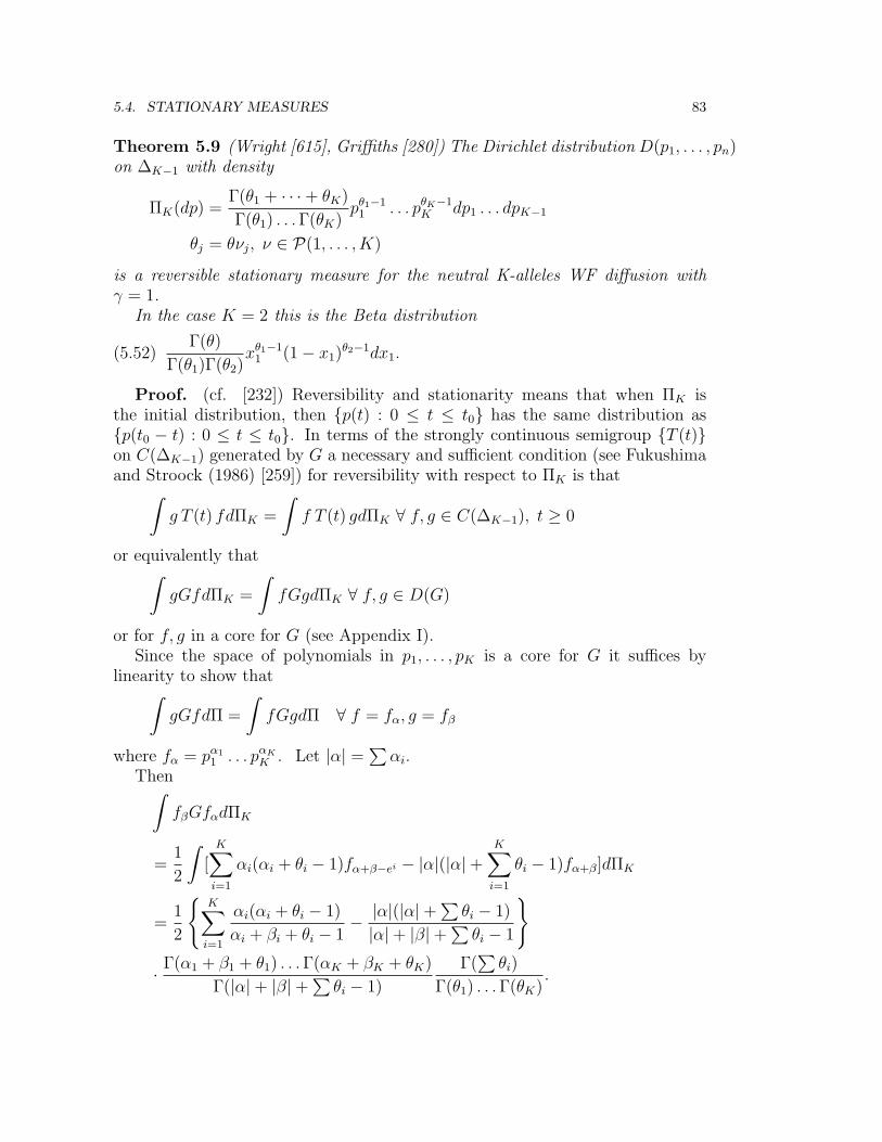
Theorem 5.9 (Wright [615], Griffiths [280]) The Dirichlet distribution D(p1, . . . , pn)on ∆K−1 with density

ΠK(dp) =Γ(θ1 + · · ·+ θK)

Γ(θ1) . . .Γ(θK)pθ1−1

1 . . . pθK−1K dp1 . . . dpK−1

θj = θνj, ν ∈ P(1, . . . , K)

is a reversible stationary measure for the neutral K-alleles WF diffusion withγ = 1.

In the case K = 2 this is the Beta distribution

(5.52)Γ(θ)

Γ(θ1)Γ(θ2)xθ1−1

1 (1− x1)θ2−1dx1.

Proof. (cf. [232]) Reversibility and stationarity means that when ΠK isthe initial distribution, then p(t) : 0 ≤ t ≤ t0 has the same distribution asp(t0 − t) : 0 ≤ t ≤ t0. In terms of the strongly continuous semigroup T (t)on C(∆K−1) generated by G a necessary and sufficient condition (see Fukushimaand Stroock (1986) [259]) for reversibility with respect to ΠK is that∫

g T (t) fdΠK =

∫f T (t) gdΠK ∀ f, g ∈ C(∆K−1), t ≥ 0

or equivalently that∫gGfdΠK =

∫fGgdΠK ∀ f, g ∈ D(G)

or for f, g in a core for G (see Appendix I).Since the space of polynomials in p1, . . . , pK is a core for G it suffices by

linearity to show that∫gGfdΠ =

∫fGgdΠ ∀ f = fα, g = fβ

where fα = pα11 . . . pαKK . Let |α| =

∑αi.

Then∫fβGfαdΠK

=1

2

∫[K∑i=1

αi(αi + θi − 1)fα+β−ei − |α|(|α|+K∑i=1

θi − 1)fα+β]dΠK

=1

2

K∑i=1

αi(αi + θi − 1)

αi + βi + θi − 1− |α|(|α|+

∑θi − 1)

|α|+ |β|+∑θi − 1

· Γ(α1 + β1 + θ1) . . .Γ(αK + βK + θK)

Γ(|α|+ |β|+∑θi − 1)

Γ(∑θi)

Γ(θ1) . . .Γ(θK).


To show that this is symmetric in α, β, let h(α, β) denote the expression within... above. Then

h(α, β)− h(β, α)

=∑ α2

i − β2i + (αi − βi)(θi − 1)

αi + βi + θi − 1− |α|

2 − |β|2 + (|α| − |β|)(∑θi − 1)

|α|+ |β|+∑θi − 1

=∑

(αi − βi)− (|α| − |β|)= 0

Corollary 5.10 Consider the mixed moments:

mk1,...kK =

∫. . .

∫∆K−1

pk11 . . . pkKK ΠK(dp)

Then

mk1,...kK =Γ(θ1) . . .Γ(θK)

Γ(θ1 + · · ·+ θK)

Γ(θ1 + · · ·+ θK + k1 + · · ·+ kK))

Γ(θ1 + k1) . . .Γ(θK + kK).

Stationary measure with selection

If selection (as in (5.44) is added then the stationary distribution is given by the“Gibbs-like” distribution

(5.53) Πσ(dp) = C exp

(K∑

i,j=1

σijpipj

)ΠK(dp1 . . . dpK−1)

and this is reversible. (This is a special case of a result that will be proved in alater section.)

5.4.2 Convergence of stationary measures of pNN∈N

It is of interest to consider the convergence of the stationary measures of theWright-Fisher Markov chains to (5.53). A standard argument applied to theWright-Fisher model is as follows.

Theorem 5.11 Convergence of Stationary Measures. Assume that the diffusionlimit, p(t), has a unique invariant measure, ν and that νN is an invariant measurefor pN(t). Then

(5.54) νN =⇒ ν as N →∞.

5.4. STATIONARY MEASURES 85

Proof. Denote by Ttt≥0 the semigroup of the Wright-Fisher diffusion. Sincethe state space is compact, the space of probability measure is compact. andtherefore the sequence νN is tight M1(∆K−1). Given a limit point ν and asubsequence νN ′ that converges weakly to ν ∈ M1(∆K−1) it follows that forf ∈ C(∆K−1),∫

T (t)fdν = limN ′→∞

∫T (t)fdνN ′ (by νN ′ =⇒ ν)

= limN ′→∞

∫TN ′(2N

′t)fdνN ′ (by pN =⇒ p)

= limN ′→∞

∫fdνN ′ (by inv. of νN ′)

=

∫fdν (by νN ′ =⇒ ν).

Therefore ν is invariant for T (t) and hence ν = ν by assumption of the unique-ness of the invariant measure for p(t). That is, any limit points of νN coincideswith ν and therefore νN =⇒ ν.

Properties of the Dirichlet Distribution

1. Consistency under merging of types.Under D(θ1, . . . , θn), the distribution of (X1, . . . , Xk, 1− Σk

i=1Xi) is

D(θ1, . . . , θk, θk+1 + · · ·+ θn)

and the distribution of Xk1−Σk−1

i=1 Xi= Xk

ΣKi=kXiis Beta(θk,Σ

Ki=k+1θi).

2. Bayes posterior under random samplingConsider the n-dimensional Dirichlet distribution, D(α) with parameters (α1, . . . , αn).

Assume that some phenomena is described by a random probability vector p =(p1, . . . , pn). Let D(α) be the “prior distribution of the vector p. Now let usassume that we take a sample and observe that Ni of the outcome are i. Nowcompute the posterior distribution of p given the observations N = (N1, . . . , Nn)as follows: Using properties of the Dirichlet distribution we can show that it is

P (p ∈ dx|N) =1

Z

xα11 . . . xαnn xN1

1 . . . xNnn∫xα1

1 . . . xαnn xN11 . . . xNnn dx1 . . . dxn

=1

Z ′x

(α1+N1)1 . . . x(αn+Nn)

n .

That is,

(5.55) P (p ∈ ·|N) is D(α1 +N1, . . . , αn +Nn).

Chapter 18

Appendix III: Markov Processes

18.1 Operator semigroups

See Ethier-Kurtz, [222] Chap.1.

Consider a strongly continuous semigroup Tt with generator G and domainD(G). A subset D0 ⊂ D(G) is a core if the closure of G|D0 equals G. If D0 isdense and Tt : D0 → D0 for all t, then it is a core.

Theorem 18.1 (Kurtz semigroup convergence Theorem [222], Chap. 1, Theo-rem 6.5) Let L,Ln be Banach spaces and πn : L→ Ln is a bounded linear mappingand supn ‖πn‖ <∞. We say fn ∈ Ln → f ∈ L if limn→∞ ‖fn − πnf‖ = 0.

For n ∈ N let Tn be a contraction on a Banach space Ln, let εn > 0, limn→∞ εn =0. Let T (t) be a strongly continuous contraction semigroup on L with generatorA and let D be a core for A. Then the following are equivalent:

(a) For each f ∈ L, Tbt/εncn πnf → T (t)f, for all t ≥ 0, uniformly on bounded

intervals.

(b) For each f ∈ D there existsfn ∈ Ln such that fn → F and Anfn → Af .

Theorem 18.2 [222] Chap. 4, Theorem 2.5.Let E be locally compact and separable. For n = 1, 2, . . . let Tn(t) be a Fellersemigroup on C0(E) and suppose that Xn is a Markov process with semigroupTn(t) and sample paths in DE([0,∞)). Suppose that T (t) is a Feller semi-group on C0(E) such that for each f ∈ C0(E)

(18.1) limn→∞

Tn(t)f = T (t)f, t ≥ 0.

If Xn(0) has limiting distribution ν ∈ P(E), then there is a Markov process Xcorrespondng to T (t) with initial distribution ν and sample paths in DE([0,∞))with initial distribution ν and sample paths in DE([0,∞)) and Xn ⇒ X.

355

17.4. TOPOLOGIES ON PATH SPACES 347

17.4 Topologies on path spaces

Definition 17.9 Let µi, µ ∈ Mf . Then (µn)n∈N converges weakly to µ as n →∞, denoted µn ⇒ µ iff and only is

(17.7)

∫fdµn=⇒

n→∞

∫fdµ ∀ f ∈ Cb(E)

Given a Polish space (E, d) we consider the space CE([0,∞)) with the metric

(17.8) d(f, g) =∞∑n=1

2−n sup0≤t≤n

|f(t)− g(t)|.

Then (CE([0,∞), d) is also a Polish space. To prove weak convergence in P((CE([0,∞), d))it suffices to prove tightness and the convergence of the finite dimensional distri-butions.

Similarly the space DE([0,∞) of cadlag functions from [0,∞) to E with the

Skorohod metric d is a Polish space where

(17.9) d(f, g) = infλ∈Λ

(γ(λ) +

∫ ∞0

e−u(

1 ∧ suptd(f(t ∧ u), g(t ∧ u))

))where Λ is the set of continuous, strictly increasing functions on [0,∞) and forλ ∈ Λ,

(17.10) γ(λ) = 1 +

(supt|t− λ(t)| ∨ sup

s 6=t| log(λ(s)− λ(t))

s− t|).

Theorem 17.10 (Ethier-Kurtz) (Ch. 3, Theorem 10.2) Let Xn and X be pro-cesses with sample paths in DE([0,∞) and Xn ⇒ X. Then X is a.s. continuousif and only if J(Xn)⇒ 0 where

(17.11) J(x) =

∫ ∞0

e−u[ sup0≤t≤u

d(X(t), x(t−))].

17.4.1 Sufficient conditions for tightness

Theorem 17.11 (Aldous (1978)) Let Pn be a sequence of probability measureson D([0,∞),R) such that

• for each fixed t, Pn X−1t is tight in R,

• given stopping times τn bounded by T <∞ and δn ↓ 0 as n→∞

(17.12) limn→∞

Pn(|Xτn+δn −Xτn| > ε) = 0,

or

APPENDIX FOR LECTURE 6

348 CHAPTER 17. APPENDIX II: MEASURES AND TOPOLOGIES

• ∀ η > 0 ∃δ, n0 such that

(17.13) supn≥n0

supθ∈[0,δ]

Pn(|Xτn+θ −Xτn| > ε) ≤ η.

Then Pn are tight.

17.4.2 The Joffe-Metivier criteria for tightness of D-semimartingales

We recall the Joffe Metivier criterion ([352]) for tightness of locally square inte-grable processes.

A cadlag adapted process X, defined on (Ω,F ,Ft, P ) with values in R iscalled a D-semimartingale if there exists a cadlag function A(t), a linear subspaceD(L) ⊂ C(R) and a mapping L : (D(L)×R× [0,∞)×Ω)→ R with the followingproperties:

1. for every (x, t, ω) ∈ R× [0,∞)×Ω the mapping φ→ L(φ, x, t, ω) is a linearfunctional on D(L) and L(φ, ·, t, ω) ∈ D(L),

2. for every φ ∈ D(L), (x, t, ω) → L(φ, x, t, ω) is B(R)× P-measurable, whereP is the predictable σ-algebra on [0,∞)× Ω, (P is generated by sets of theform (s, t]× F where F ∈ Fs and s, t are arbitrary)

3. for every φ ∈ D(L) the process Mφ defined by

(17.14) Mφ(t, ω) := φ(Xt(ω)− φ(X0(ω))−∫ t

0

L(φ,Xs−(ω), s, ω)dAs,

is a locally square integrable martingale on (Ω,F ,Ft, P ),

4. the functions ψ(x) := x and ψ2 belong to D(L).

The functions

(17.15) β(x, t, ω) := L(ψ, x, t, ω)

(17.16) α(x, t, ω) := L((ψ)2, x, t, ω)− 2xβ(x, t, ω)

are called the local characteristics of the first and second order.

Theorem 17.12 Let Xm = (Ωm,Fm,FMt , Pm) be a sequence of D-semimartingaleswith common D(L) and associated operators Lm, functions Am, αm, βm. Then thesequence Xm : m ∈ N is tight in DR([0,∞) provided the following conditionsare satisfied:

1. supmE|Xm0 |2 <∞,


2. there is a K > 0 and a sequence of positive adapted processes Cmt : t ≥ 0 on Ωmm∈N

such that for every m ∈ N, x ∈ R, ω ∈ Ωm,

(17.17) |βm(x, t, ω)|2 + αm(x, t, ω) ≤ K(Cmt (ω) + x2)

and for every T > 0,

(17.18) supm

supt∈[0,T ]

E|Cmt | <∞, and lim

k→∞supmPm( sup

t∈[0,T ]

Cmt ≥ k) = 0,

3. there exists a positive function γ on [0,∞) and a decreasing sequence ofnumbers (δm) such that limt→0 γ(t) = 0, limm→∞ δm = 0 and for all 0 < s < tand all m,

(17.19) (Am(t)− Am(s)) ≤ γ(t− s) + δm.

4. if we set

(17.20) Mmt := Xm

t −Xm0 −

∫ t

0

βm(Xms−, s, ·)dAms ,

then for each T > 0 there is a constant KT and m0 such that for all m ≥ m0,then

(17.21) E( supt∈[0,T ]

|Xmt |2) ≤ KT (1 + E|Xm

0 |2),

and

(17.22) E( supt∈[0,T ]

|Mmt |2) ≤ KT (1 + E|Xm

0 |2),

Corollary 17.13

Assume that for T > 0 there is a constant KT such that

(17.23) supm

supt≤T,x∈R

(|αm(t, x)|+ |βm(t, x)|) ≤ KT , a.s.

(17.24)∑m

(Am(t)− Am(s)) ≤ KT (t− s) if 0 ≤ s ≤ t ≤ T,

and

(17.25) supmE|Xm

0 |2 <∞,

and Mmt is a square integrable martingale with supmE(|Mm

T |2) ≤ KT . The theXm : m ∈ N are tight in DR([0,∞).


Criteria for continuous processes

Now consider the special case of probability measures on C([0,∞),Rd). Thiscriterion is concerned with a collection (X(n)(t))t≥0 of semimartingales with valuesin Rd with continuous paths. First observe that by forming

(17.26) (< X(n)(t), λ >)t≥0 , λ ∈ Rd

we obtain R-valued semi-martingales. If for every λ ∈ Rd the laws of theseprojections are tight on C([0,∞),R) then this is true for [L[(X(n)(t))t≥0], n ∈ N.The tightness criterion for R-valued semimartingales is in terms of the so-calledlocal characteristics of the semimartingales.

For Ito processes the local characteristics can be calculated directly from thecoefficients. For example, if we have a sequence of semimartingales Xn that arealso a Markov processes with generators:

(17.27) L(n)f =( d∑i=1

ani (x)∂

∂xi+

d∑i=1

d∑j=1

bni,j(x)∂2

∂xi∂xj

)f

then the local characteristics are given by

(17.28) an = (ani )i=1,··· ,d, bn = (bni,j)i,j,=1,··· ,d.

The Joffe-Metivier criterion implies that if

supn

sup0≤t≤T

E[(|an(X(n)(t)|+ |bn(X(n)(t)|)2] <∞,(17.29)

limk→∞

supnP ( sup

0≤t≤T(|an(X(n))(t)|+ |bn(X(n))(t)|) ≥ k) = 0(17.30)

then L[(X(n)(t))t≥0], n ∈ N are tight in C([0,∞),R). See [352] for details.

Theorem 17.14 (Ethier-Kurtz [225] Chapt. 3, Theorem 10.2) Let

(17.31) J(x) =

∫ ∞0

e−u[J(x, u) ∧ 1]du, J(x, u) = sup0≤t≤u

d(x(t), x(t−)).

Assume that a sequence of processes Xn ⇒ X in DE([0,∞)). Then X is a.s.continuous if and only if J(Xn)⇒ 0.

17.4.3 Tightness of measure-valued processes

Lemma 17.15 (Tightness Lemma).(a) Let E be a compact metric space and Pn a sequence of probability measureson D([0,∞),M1(E)). Then Pn is compact if and only if there exists a linearseparating set D ⊂ C(E) such that t →

∫f(x)Xt(ω, dx) is relatively compact in

D([0,∞), [−‖f‖, ‖f‖]) for each f ∈ D.


(b) Assume that Pn is a family of probability measures on D([0,∞), [−K,K])such that for 0 ≤ t ≤ T , there are bounded predictable processes vi(·) : i = 1, 2such that for each n

Mi,n(t) := x(ω, t)i −∫ t

0

vi,n(ω, s)ds, i = 1, 2

are Pn-square integrable martingales with

supnEn(sup

s(|v2,n(s)|+ |v1,n(s)|)) <∞.

Then the family Pn is tight.(c) In (b) we can replace the i = 2 condition with: for any ε > 0 there exists fand vf,n such that

sup[−K,K]

|fε(x)− x2| < ε

and

Mf,n(t) := fε(x(ω, t))−∫ t

0

vfε,n(ω, s)ds

supnEn(sup

s(|vfε,n(s)|) <∞.

Proof. (a) See e.g. Dawson, [139] Section 3.6.(b) Given stopping times τn and δn ↓ 0 as n→∞.

En[(x(τn + δn)− x(τn))2

]= En[x2(τn + δn)− x2(τn)]− 2En[x(τn)(x(τn + δn)− xn(τn))]

≤ En[

∫ τn+δn

τn

|v2,n(s)|ds+ 2K

∫ τn+δn

τn

|v1,n(s)|ds]

≤ δn supnEn(sup

s(|v2,n(s)|+ |v1,n(s)|))

→ 0 as δn → 0.

The result then follows by Aldous’ condition.(c)

En[(x(τn + δn)− x(τn))2

]= En[x2(τn + δn)− x2(τn)]− 2En[x(τn)(x(τn + δn)− xn(τn))]

≤ En(f(x(τn + δn))− f(x(τn))) + 2K

∫ τn+δn

τn

|v1,n(s)|ds] + 2ε

≤ En[

∫ τn+δn

τn

|vfε,n(s)|ds+ 2K

∫ τn+δn

τn

|v1,n(s)|ds] + 2ε

≤ δn supnEn(sup

s(|vfε,n(s)|+ |v1,n(s)|)) + 2ε


Hence for any ε > 0

limδn→0

supnEn[(x(τn + δn)− x(τn))2

]≤ lim

n→∞δn sup

nEn(sup

s(|vfε,n(s)|+ |v1,n(s)|)) + 2ε

= 2ε.

and the result again follows from Aldous criterion.

Remark 17.16 These results can be also used to prove tightness in the case ofnon-compact E. However in this case an additional step is required, namely toshow that for ε > 0 and T > 0 there exists a compact subset KT,ε ⊂ E such that

Pn[D([0, T ], KT,ε)] > 1− ε ∀ n.

Remark 17.17 Note that if Pn is a tight sequence of probability measures onD([0, T ],R) such that Pn(sup0≤s≤T |x(s) − x(s−)| ≤ δn) = 1 and δn → 0 as n→∞, then for any limit point P∞, P∞(C([0, T ],R)) = 1.

17.5 The Gromov-Hausdorff metric on the space of com-pact metric spaces

Let E be a metric space and B1, B2 two subsets. Then the Hausdorff distance isdefined by

(17.32) dH(K1, K2) = infε ≥ 0 : K1 ⊂ Vε(K2), K2 ⊂ Vε(K1)

where Vε(K) denotes the ε-neighbourhood of K. This defines a pseudometric,dH(B1, B2) = 0 iff they have the same closures.

If X and Y are two compact metric spaces. The Gromov-Hausdorff metricdGH(X, Y ) is defined to be the infimum of all numbers dH(f(X), g(Y )) for allmetric spaces M and all isometric embeddings f : X → M and g : Y → M andwhere dHaus denotes Hausdorff distance between subsets in M. dGH is a pseudo-metric with dGH(K1, K2) = 0 iff they are isometric.

Now let (K, dGH) denote the class of compact metric spaces (modulo isometry)with the Gromov-Hausdorff metric. Then (K, dGH) is complete.

See Gromov [289] and Evans [235] for detailed expositions on this topic.

17.5.1 Metric measure spaces

The notion of metric measure space was developed by Gromov [289] (called mmspaces there). It is given by a triple (X, r, µ) where (X, r) is a metric space suchthat (supp(µ), r) is complete and separable and µ ∈ P(X) is a probability measure

17.5. THE GROMOV-HAUSDORFF METRIC ON THE SPACE OF COMPACT METRIC SPACES353

on (X, r). Let M be the space of equivalence classes of metric measure spaces(whose elements are not themselves metric spaces - see remark (2.2(ii)) in[287])with equivalence in the sense of measure-preserving isometries. The distancematrix map is defined for n ≤ ∞

(17.33) Xn → R(

n2

)

+ , ((xi)i=1,...,n)→ (r(xi, xj))1≤i<j≤n

and we denote by R(X, r) the map that sends a sequence of points to its infinitedistance matrix.

Then the distance matrix distribution of (X, r, µ) (representative of equiva-lence class) is defined by

(17.34) ν(X,r,µ) := R(X,r) − pushforward of µ⊗N ∈ P(R

N2

+ ).

Since this depends only on the equivalence class it defined the mapping κ→ νκ

for κ ∈ M. Gromov [289] (Section 312.5) proved that a metric measure space is

characterized by its distance matrix distribution.Greven, Pfaffelhuber and Winter (2008) [287] introduced the Gromov-weak

topology. In this topology a sequence χn converges Gromov-weakly to χ in Mif and only if Φ(χn) converges to Φ(χ) in R for all polynomial in Π.

In [287], Theorem 1, they proved that M equipped with the Gromov-weaktopology is Polish.

An important subclass is the set of ultrametric measure spaces given by theclosed subset of M

(17.35) U := u∈M : u is ultra-metric.

wright-fisher processesdb5d/summerschool09/lectures-dd/lectures6-7.pdf · wright-fisher markov...

Documents