DYNAMICS OF WAITING IN PIGEONS

C. D. L. WYNNE, J. E. R. STADDON, AND J. D. DELI US

UN IVERS ITY OF WESTERN AUSTRALIA. DUKE UN IVERSITY. AN D UNIVERSITAT KONSTANZ

Two experiments used response-in itiated delay schedules to test the idea that when food reinforce­ment is available a t regular intervals, the time an animal waits before its fi rst operant response (waiting time) is proportional to the immediately preceding intedood interval (linear waiting; Wynne & Staddon . 1988). In Experiment 1 the interfood intervals varied from cycle to cycle acco rding to one of four sinusoidal sequences with different amounts of added noise. Waiting times tracked the input cycle in a way which showed that they were affected by interfood intervals earlier th an the immediately preceding one. In Experiment 2 different patterns of long and short interfood intervals were presented, and th e results implied tha t waiting times are disproportionately inf1uenced by the shortest of recent interfood intervals. A model based on this idea is shown to acco unt for a wide range of results on the dynamics of timing behavior.

Key words: linear waiting, temporal discrimination , sequential analysis, cycl ic-interval sc hedules, response-initiated delay schedules, key peck, pigeons

When an hedonic event such as a food de­livery to a hungry subject occurs at regular intervals, behavior often reflects this period­icity. This was demonstrated in Pavlov's labo­ratory at the turn of the century (Feokritova, 1912, cited in Pavlov, 1928), and it has been much studied since, in both operant and Pav­lovian settings (see Richelle & Lejeune, 1980, ror a review). Recently, Staddon, Wynne, and Higa (1991), expanding on a suggestion of Ferster and Skinner (1957), argued that ad­aptation to temporal constraints may be re­sponsible for the typical patterns of respond­ing observed on many different schedules of reinforcement, not just those in which time is explicitly programmed (e.g., interval sched­ules) .

After sufficient experience on periodic food schedules (such as fixed interval or fixed time), subjects usually develop a pattern of responding that takes the form of a post-

Our thanks to Nancy Innis and Armando Machado for Ilelpful comments on earlier drafts of this paper, and to

David Young for a most useful discussion leading to the development of Experiment 2. Research was supported by grants to Duke University from the National Science Foundation and National Institute of Mental Health and to J. D. Delius from the Deutsche Forschungsgemein­'chaft. C. D. L. Wynne gratefully acknowledges support "rom a NATO postdoctoral fellowship and the Alexander "on Humboldt-Stiftung, and J. E. R. Staddon also thanks \IATO and the von Humboldt-Stiftung for support.

Address correspondence to C. D. L. Wynne at the Department of Psychology, University of Western Austra­lia, Nedlands, Western Australia 6009, Australia (E-mail: d ive@psy.uwa.edu.au) .

reinforcement pause or waiting time in each interfood interval (IFI) before operant re­sponding begins. This waiting time is typically proportional to the IFI (Schneider, 1969). Skinner (1938) observed that "With a re la­tively short period of [temporal condition­ing] depressions [i.e., postreinforcement pauses] begin to appear within a few days" (p. 125) . He also noted that when the IFI was long, the development of pausing was "sub­stantially retarded." Because of this lag in ad­aptation, most research on temporal sched­ules has centered on the steady-state properties of the behavior. In contrast, the present study tests an hypothesis about the dynamics of the process of initial adaptation to temporal schedules.

Several recent studies (Higa, Thaw, & Stad­don, 1993; Higa, Wynne, & Staddon, 1991; Innis, Mitchell, & Staddon, 1993; Wynne & Staddon, 1988, 1992) have looked at the dy­namics of the pausing process in pigeons us­ing response-initiated delay (RID) schedules (technically, signaled chain or conjunctive fixed-ratio [FR] 1 fixed-time [FT] schedules). As shown in Figure 1, each IFI starts with the single response key illuminated red. A re­sponse to this key causes it to turn green for a schedule-controlled time (the food delay, 1) prior to the delivery of food . The next IFI follows directly.

Wynne and Staddon (1988, 1992) showed that on these RID schedules, pigeons pause an approximately fixed fraction of the in ter­food interval I (where I is just the sum of the

603

604

first response

Food Red Green Food

•••• waiting time (pause), t food delay, T .... • .... •

........ ----Interfood Interval, I Fig. l. One IF! of the response-initiated delay (RID) schedule .

waltmg time, t, plus the subsequent pro­grammed delay, 7) , irrespective of how the relationship between food delay and waiting time is programmed. Indeed, despite the col­or change on first response to a RlD sched­ule, several studies have shown that waiting times so obtained are indistinguishable from those found on regular fixed-interval (FI) schedules in which the first response has no stimulus consequences (Shull, 1970; Wynne & Staddon , 1992). Innis et al. (1993) and Wynne and Staddon (1992) also demonstrat­ed that waiting times on RID schedules are controlled by the IFI, and not the food delay, T (but see Capehart, Eckerman, Guilkey, & Shull, 1980). Moreover, the pigeons' waiting times tracked the IFls even when these varied from trial to trial (Higa et aI., 1991; Innis et aI. , 1993). Little sign was found of the gradual adjustment to each new IFI observed by Fers­ter and Skinner (1957). This suggested that at least some part of the dynamic process that allows adaptation to temporal schedules might be quite rapid. We termed this rapid adapta­tion of waiting times to IFls obligatory linear waiting (Wynne & Staddon, 1988). The aim of the present experiments is to better under­stand this fast-acting process. We attempt to minimize the effects of slower processes by changing session parameters frequently.

The simplest theoretical possibility is that waiting is strictly a one-back process: Waiting time in IFI N + 1 is some function of the duration of the preceding IFI, N, that is, tN+ I

= f(lN)' The simplest form of dependence is linear, so the one-back linear-waiting hypoth­esis is just that:

tN+ 1 = AI.¥ + B, (1)

where A is the constant of proportionality (0 < A < 1) and B is a constant intercept of negligible magnitude (modal values from previous studies are A = 0.2, B = 0).

Wynne and Staddon (1988) tested a coun­terintuitive prediction of this hypothesis us­ing an "autocatalytic" RlD schedule in which the programmed delay, T was set proportion­al to the preceding IFI: TN+ 1 = w!'v. We argued that if waiting time, tN+ 1, is proportional to

the preceding IFI, only two outcomes are pos­sible, depending on the value of the constant w. If w > 1/ A, waiting times in successive in­tervals should get longer and longer; if w < 1/ A, waiting times should get shorter and shorter.

The results were in partial agreement with these predictions. At low values of w, waiting times were very short; at high values of w, waiting times were long and tended to in­crease in runs. But the fact that subjects rare-

Iy stopped responding completely when ex­posed to large w values implies that the preceding IFI is not the only determinant of waiting time. Our data are consistent with a dependence of waiting time on, for example , the weighted sum of the previous M IFIs (B is assumed to be negligible):

M

tN+ 1 = 2 AJN- k, k=O

(2)

where Ak are weights for each IF! £i·om 0 to M . The aim of the present experiments was to

explore the dependence of waiting time on preceding IFIs in the RID procedure. Our strategy was to present the pigeons with food delays that varied within a session, and to an­alyze the obtained waiting times to determine how they were influenced by IFIs further back in the past. In the first experiment we varied the duration of T from IFI to IF! in a more or less regular manner and then used simu­lations to see if waiting time, tN + I , tracked IFI, IN, in a manner consistent with one-back lin­ear waiting, or whether the results implied ef­fects of IFIs further back in the series. The second experiment allowed tests of specific hypotheses about how IFIs combine to influ­ence waiting times.

EXPERIMENT 1: CYCLIC IFIS WITH

ADDED NOISE

Several previous studies have shown that when IFIs vary regularly within a session, the pauses produced by pigeons track these changes (Higa et aI., 1991; Innis, 1981; Innis et aI., 1993; Innis & Staddon, 1970, 1971) . Our aim here is to use this method to uncov­er the details of the dynamics of this process. Is waiting time controlled by IFIs in trials ear­lier than the immediately preceding one (is M > 0 in Equation 2)? We approach this question here by simulating the results to be expected on the basis of Equations 1 and 2 and comparing them with obtained waiting times from different input series.

Method

SubJects. Four experimentally experienced, locally acquired homing pigeons (Columba liv­ia) of racing stock were used. They were held at 80% of their free-feeding weights by limit­ing access to food.

605

Apparatus. The experiment was run in a one­key cubic steel Skinner box with internal di­mensions 33 cm on a side. A single response key (2.5 cm diameter), which could be transil­luminated with red or green light, was mount­ed 21 cm above the floor in the center of the back panel. The food-hopper opening (2 em diameter), set 7 em above the floor in the cen­ter of the back wall, gave access to mixed food grains when the food hopper was raised. A houselight in the ceiling gave background il­lumination throughout the experiment. There was no need for a hopper lig ht because the hopper opening projected 3 cm into the cham­ber. Food reward was 2-s access to mixed grains. A Commodore® VIC-20 microcomputer con­trolled experimental events and recorded the times of key pecks. Data were transferred to a larger computer for analysis.

Procedure. Each experimental session consist­ed of 100 IFIs of the RID procedure described above, one IFI of which is shown in Figure 1. In this experiment delay time, T, in the pres­ence of the green stimulus varied from IF! to IF! according to the sinusoidal rule:

TN= 10 + 5sin(2Nrr/ l00) + E, (3)

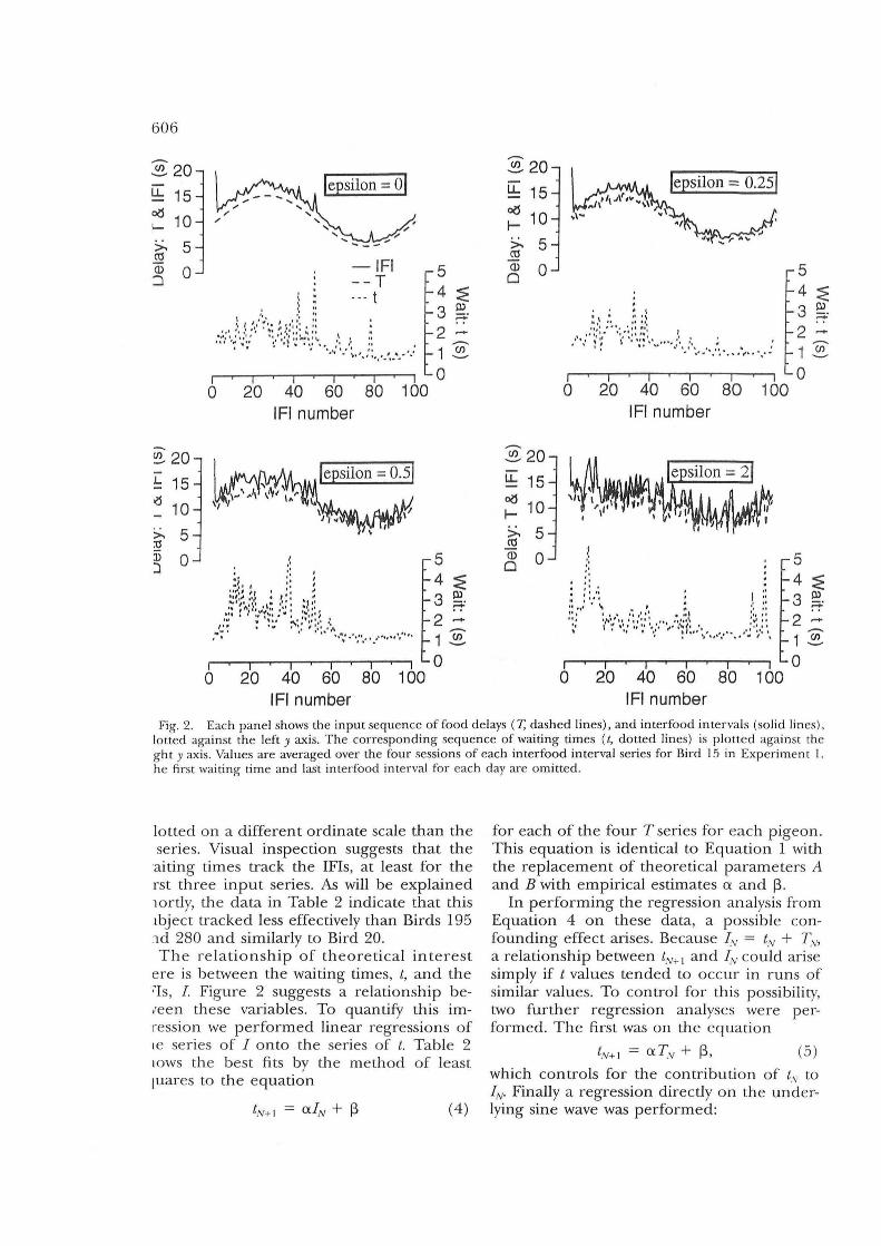
where N is IFI number and E is a noise term. Thus, when E = 0, successive values of T in a session followed a single cycle of a sine wave with a mean of 10 s and a range of 5 to 15 s. For the other three conditions, E was derived by sampling from a rectangular random dis­tribution ranging from 0 to 0.25, 0 to 0.5, or o to 2. In order to maintain a constant range of T values, each of the three T series ob­tained in this way was normalized to keep the overall range between 5 and 15 s. The four T series thus represent successively more de­graded versions of the pure sine wave that comprised Condition 1. The four input series are the dashed lines in Figure 2. Each subject received one of these four T series each day so that each value was presented four times per subject. The order of the different series was quasi-randomized, as shown in Table 1.

Results

The key data here are the obtained series of waiting times (t values) for each T series. Figure 2 shows the four programmed T se­ries, the mean series of waiting times, t, and the series of IFIs, I (the sum of the other two series) for Bird 15. The T and I series are

606

~20 u.. 15

~ 10

:>. 5 co Q5 0 :J

~

~ 20 .L 15

~ 10 >. 5 :u j) 0 )

- IFI --T " "" t

I I I I I I o 20 40 60 80 1 00 IFI number

I I I I I I o 20 40 60 80 1 00 IFI number

~20 u.. 15

06 10 f-

>- 5 co (]) 0 o

~20 u.. 15

~ 10

>- 5 co (]) 0 o

I I I I I I o 20 40 60 80 100

IFI number

I I I I I I o 20 40 60 80 1 00

IFI number

5 4 ~ 3 ~ 2 1~ o

Fig. 2. Each panel shows the input sequence of food delays (T, dashed lines) , and interfood intervals (solid lines), lotted against the left y axis. The corresponding sequence of waiting times (/, dotted lines) is plotted against the ght y axis, Values are averaged over the four sessions of each interfood interval series for Bird 15 in Experiment '1. he first waiting time and lasl interfood interval for each day are omitted.

lotted on a different ordinate scale than the series. Visual inspection suggests that the

aiting times track the IFIs, at least for the rst three input series, As will be explained lOrtly, the data in Table 2 indicate that this lbject tracked less effectively than Birds 195 ld 280 and similarly to Bird 20, The relationship of theoretical interest

ere is between the waiting times, t, and the ~Is, I. Figure 2 suggests a relationship be­,een these variables, To quantify this im­ression we performed linear regressions of Ie series of I onto the series of t, Table 2 lOWS the best fits by the method of least luares to the equation

(4)

for each of the four T series for each pigeon. This equation is identical to Equation 1 with the replacement of theoretical parameters A and B with empirical estimates ex and 13,

In performing the regression analysis from Equation 4 on these data, a possible con­founding effect arises, Because Iv = t.v + T.v, a relationship between tv+ I and IN could arise simply if t values tended to occur in runs of similar values, To control for th is possibility, two further regression analyses were per­formed, The first was on the equation

(5) which controls for the contribution of t v to IN' Finally a regression directly on the under­lying sine wave was performed:

Table 1

Sequence of E parameters for each pigeon in Experi-ment I.

Condition Bird

(day) 15 20 195 280

0 2 0.5 0.25 2 0.25 0.5 2 0 3 0.5 0.25 0 2 4 2 0 0.25 0.5 .') 0 2 0.5 0.25 6 0.25 0.5 2 0 7 0.5 0.25 0 2 8 2 0 0.25 0.25 9 0 2 0.5 0.5

10 0.25 0.5 2 0 II 0.5 0.25 0 2 12 2 0 0.25 0.5 13 0 2 0.5 0.25 14 0.25 0.5 2 0 15 0.5 0.25 0 2 16 2 0 0.25 0.5

tN+ I = exsin(2N'TT/ 100) + [3. (6)

This tests whether the tracking by t values is really of the underlying sinusoid.

The results of these regression analyses for all subj ects are shown in Table 2. Consider first the proportions of variance accounted for ( r) by the three regression equations. Most of these values are similar for the three different regressions. It is not the case that the regressions of t onto I are inflated relative to the regressions of tonto T or the under­lying sinusoid. Indeed, usually the regressions onto I produce lower r values than do the other two regression equations, indicating that there can be no inflation of these values due to the relationship between tN and IN'

Table 2 shows three things about the rela­tionship between tN+ I and IN' First, [3 is never significantly different from zero (except for Bird 195 in Condition E = 2; see the 95% con­fidence intervals). Second, values of ex are around 0.2 (a little lower for Bird 15), a value compatible with what has been found in pre­vious studies (Higa et al., 1991; Wynne & Stad­don, 1988, 1992). Third, the proportion of variance (r) accounted for by each regression equation decreases as the value of E increases (i.e., the noisier series are less well fitted by this model). The relationship between rand E is included in the bottom panel of Figure 3.

The relationship between r and E for the regression onto I shown in Table 2 and Figure

60 -:-

3 does not appear to be consistent with a sim­ple one-back process. Intuitively, a one-back process should be able to track a noisy IF! se­ries just as well as a smooth one. Our data, on the contrary, show that the larger the value 0 1

the noise term, E, the poorer the tracking. However, intuition is often a poor guide, es­pecially because we must also take into account that, in addition to the noise in the IFI series. the linear waiting process will itself be noisy. We therefore performed a number of simulations of different types of noisy linear waiting, to see how the pattern of correlations for the simu­lated data compared with the correlations from the pigeon data at different values of the E pa­rameter. The pattern of results from all models assuming an influence of IFIs further than one back (M > 0 in Equation 2) converged on an analogous relationship between r and E, and therefore we present here the results from just two noisy models: a one-back process and a three-back process (M = 2 in Equation 2) . Our method was to generate simulated data with these two processes and compare the pattern of correlations between simulated tN+ I and I , with those obtained from the pigeon data.

In the first simulation, a t series was created from a noisy first order linear waiting process according to Equation 7:

tN+ I = (A + T)lN' (7 )

This is simply Equation 1 with B = 0 and the addition of a Gaussian noise term T . A, the constant of proportionality, was set equal to 0.20 (the relations of interest do not depend on the value of A). Note that the noise here is added to A in Equation 1 (rather than to 1) to ensure that the standard deviation of the distribution of the waiting times for constant I is proportional to their mean, as the Weber law property of temporal discrimination re­quires (cf. Gibbon, 1977; Staddon , 1965).

Our second simulation was based on Equa­tion 2, with M = 2 and Ao = Al = A2 = 0.2/ 3, and Gaussian noise added as in Equation 7. Equation 8 is an example of a three-back linear waiting process:

tN+ 1 = [(A + T) / 3](lv + IN- I + IN-2 ) ' (8 )

Figure 3 shows the r values for the regres­sions of tN+ I onto IN for each value of E. For the one-back simulation (Equation 7), we see that, with no noise in the simulation, r is 1.0 for all values of E. This illustrates the fact that

608

Bird

15

20

195

280

Table 2

Linear regression of wait series, 1."1+ 1' onto IFI series, IN> delay series, TN> and onto the under­lying sinusoid, sin (2Nrr / l00) , for each bird in Experiment 1 (ave~aged over eac h E value). Mean parameter values are shown with associated 95% confidence mtervals m brackets. dJ = 97 in all cases.

E I~ Model

0 .36 1.v+ 1 = 0.11[0.08 ~ 0.14]/."1 + 0.32[ - 0.03 --t 0.68 1

0.25 .47 l.v+1 = 0. ll[O.09--t0.13]f", + 0.23 [ -0.05 --t 0 .52]

0.5 .23 l.v+ 1 = 0.12[0.07 --t 0.16]l.v + 0.48 [ - 0.07 ~ 1.04 1

2 .10 IN+ I = 0.11 [0 .05 ~ 0.18]1."1 + 0.62[ -0.24 ~ 1.48 ]

0 .40 tN+1 =0.14[O.10~0.17]TN + 0.24[ - 0.11 ~ 0.59J

0.25 .53 1."1+1 = 0.14[0.11 ~ 0.16]TN + 0.14[ - 0.13 --t 0.41]

0.5 .34 IN+ 1 = 0.20[0.15 ~ 0.26] TN - 0.17[ - 0.78--t0.43J

2 .08 t.V+1 = 0.14[0.05 ~ 0.23] TN + 0.63[ -0.32 --t 1.58]

0 .40 t.V+ 1 = 0.68[0.51 ~ 0.84]sin(2Nrr/ 100) + 1.60[1.49 -71.72]

0.25 .50 1."1+ 1 = 0.58 [0.46 ~ 0.70]sin(2Nrr/ 100) + 1.50[1.41 --t 1.58]

0.5 .45 1."1+ 1 = 0.90[0.70 --t 1.l0]sin(2Nrr/100) + 1.92[1.78 -7 2.06]

2 .11 1."1+1 = 0.58[0.24 --t 0.92] sin (2N'TT/I00) + 2.02[1.78 -7 2.26]

0 .39 1."1+1 = 0.20[0.15 ~ 0.25]1."1 + 0.36[ - 0.37 --t 1.10]

0.25 .23 1."1+ 1 = 0.22[0.14 ~ 0.30]1."1 + 0.19[ - 0.92 --t 1.30]

0.5 .26 IN+ I = 0.20[0.1 3 ~ 0.27]1."1 + 0.41 [-0.55 --t 1.36]

2 .06 1."1+ 1 = 0.12[0.03 --t 0.21]/."1 + 1.21 [-Om --t 2.44]

0 .61 1."1+1 = 0.43 [0 .36 ~ 0.50] TN - 1.3 I[ -0.58 --t -2 .05J

0.25 .40 1."1+1 = 0.47[0.35 ~ 0.58] TN - 1.57[ - 0.38 --t - 2.75]

0.5 .37 1."1+ 1 = 0.37[0.28--t0.47]TN - 0.70[ - 1.73 --t 0.32]

2 .14 1."1+1 = 0.28]0.14 --t 0.41] TN - 0.02[ - 1.45 --t 1.41]

0 .61 1."1+ 1 = 2.16[1.82 ~ 2.51]sin(2N'TT/100) + 3.02[2.77 --t 3.26J

0.25 .39 1."1+ 1 = 2.01[1.51 --t 2.51]sin(2N'TT/100) + 3.03[2.67 --t 3.38]

0.5 .45 1."1+ 1 = 1.58[1.23 ~ 1.92]sin(2N'TT/I00) + 3.11[2.87 --t 3.36]

2 .12 1."1+1 = 0.97[0.46 ~ 1.49]sin(2N'TT/I00) + 2.73[2.36 --t 3.09]

0 .48 1."1+ 1 = 0.18[0.14 --t 0.22]1N + 0.01 [ - 0.48 --t 0 .51 ]

0.25 .43 IN+ I = 0.21 [0.16 --t 0.25]IN - 0.23[ - 0.83 --t 0 .36]

0.5 .33 IN+I = 0.17[0.12 --t 0.22]IN + O.OO[ - 0.64 ~ 0.65]

2 .14 IN+I = 0.09[0.05 --t 0.13]IN + 0.94[0.39 --t 1.50]

0 .57 1."1+ 1 = 0.26[0.21 --t 0.30] TN - 0.31 [ - 0.79 --t 0 .16]

0.25 .44 1."1+1 = 0.27[0.21 --t 0.33] TN - 0.43 [ - 1.06 --t 0.21]

0.5 .43 IN+ I = 0.27[0.21 --t 0.33] TN - 0.56[ - 1.20 --t 0.08]

2 .15 IN+ I = 0.12[0.06 --t 0.17] TN + 0.87[0.30 --t 1.45]

0 .57 1."1+1 = 1.29[1.07 --t 1.51]sin(2Nrr/l00) + 2.27 [2.11 --t 2.43]

0.25 .45 1."1+1 = 1.20[0.93 --t 1.46]sin(2Nrr/l00) + 2.25[2.07 --t 2.44]

0.5 .48 1."1+1 = 1.07[0.84 --t 1.29]sin(2Nrr/100) + 2.17[2.01 --t 2.33]

2 .29 1."1+1 = 0.60[0.42 --t 0.79]sin(2Nrr/l00) + 2.03[1.89 --t 2.16]

0 .56 1."1+1 = 0.23[0.19 --t 0.27]/."1 - 0.56[ - 1.10 --t -0.02]

0.25 .52 IN+I = 0.23 [0.19 --t 0.27]IN - 0.55[ - 1.12 --t 0.01]

0.5 .49 IN+I = 0.21[O.17--t0.25]IN - 0.37[ -0.93 --t 0.19]

2 .21 1."1+1 = 0.19[0.12 ~ 0.26]IN + 0.27[ -0.70 --t 1.23]

0 .54 1."1+1 = 0.30[0.25 --t 0.36] TN - 0.76[ -1.35 --t - 0.16]

0.25 .52 IN+I = 0.31 [0.25 --t 0.37] TN - 0.87[ -1.49 --t -0.24]

0.5 .45 IN+ I = 0.26[0.20 --t 0.32] 1 ....... - 0.42[-1.03--t0.19]

2 .21 1."1+1 = 0.24 [0.14 --t 0.33] TN + 0.29[ -0.68 --t 1.27]

0 .54 1."1+1 = 1.51 [1.23 --t 1.79]sin(2Nrr/ l00) + 2.27[2.07 --t 2.47]

0.25 .57 1."1+1 = 1.43[1.18 --t 1.67]sin(2Nrr/l00) + 2.21 [2.04 --t 2.39]

0.5 .48 IN+ I = 1.03[0.81 ~ 1.24]sin(2Nrr/100) + 2.25[2.10 --t 2.41]

2 .24 IN+ I = 0.96[0.62 --t 1.30]sin(2Nrr/l00) + 2.67[2.42 ~ 2.91 '1

a one-back process tracks all input series equally well. As we add more noise, the mo­del's ability to track is degraded: The rs are lower and decrease with increasing E, but only

up to about E = 0.5; beyond this level th( is little further decrease in the r. The fits the model decrease with increases in E up a certain level because there are autocOI

1.0

0.8

"C CD 0.6 ~

ca :::J cr

0.4 (J) I ~

0.2

0.0

1.0

0.8

"C CD 0.6 ~ ca :::J cr 0.4 (J)

I ~

0.2

0.0

1.0

0.8

"C CD 0.6 ~

ca :::J cr

0.4 (J) I ~

0.2

0.0 I o

II-back model I -.. -~ - no noise

..... -··0.04

"- -- 0.06 "­"- - - 0.08

... 0.10 ,-~~-----------------, -----," , -------- ------------- --0.12

"

, ".',

".

,

"

", , ....................................... . ' .. - - .. - - .. -_ .. - - .. - _ .. - - .. - _ .. - - ..

". ", .. , ' .. ",

". ",

'"

I 3-back model I

". ". , , ,

.. , , , , '"

, , , . , , .. , ", ".

- no noise ... 0.03 ... 0.06 _ .. 0.09 _. 0.12

" ."" ........... - ... - ... -" .... - .... -.... - ",

",

" ..... - ..... - .... -............. .. ... --. -- - -- .. ----_ .. - ... _ .. - .. ---::"--:'::"

pigeon data

--0._ ..... -...

-0- Bird 15 .+ Bird 20 -0- Bird 195 -0- Bird 280 ...... -......

' .. ' .. ---

I I 0.25 0.5

Epsilon

-- "' ...... ----__ --0 ---........ ........ .............. -+

I 2.0

609

Fig. 3. Each panel shows the goodness of fit of the regression of waiting time in cycle N + 1 ( tN+ 1) onto IFI in cycle N (IN)' Top panel: results of a one·back linear waiting simulation (Equation 5); middle panel: results of a three­back simulation (Equation 6); bottom panel: results from subjects in Experiment 1. For both simulations the numbers in the legend are the standard deviations of the noise parameter T . See text for further details.

610

lations in the sinusoid that underlies the T series. These autocorre lations in the input se­ries values inflate the input-output correla­tions at the lowest E values.

The results of the simulations of Equation 8 are plotted in the middle pane l of Figure 3. Here, the ability of the simulated t series to track th e I series is influenced by th e amount of noise in the input series even when there is no noise in the simulation; the goodness of fit of the no-noise simulation de­clines as E increases. With or without noise in the simulation, the i!s decrease throughout the range of E studied here. As expected, a more than one-back process is progressively impaired in its ability to track increasingly noisy input series.

The bottom panel of Figure 3 shows the comparable f2 values for the data from the 4 subjects in this experiment (taken from Table 2). These .y2 values decline throughout the range of E values tested, in a way that approx­imates simulations from the M = 2 model in the center paneL

Discussion

Experimen t 1 shows that pigeons can track periodically varying series of food delays, even when the series are degraded by varying amounts of noise, but the greater the noise , the worse the tracking. This degradation of the effectiven ess of tracking does not level off, as predicted by one-back linear waiting, but rather continues as more and more noise is added to the input series. This pattern is consistent with the hypothesis that current waiting time is influenced by IFIs further than one back.

These results cannot be taken as strong support for the particular more-than-one­back model simulated here (Equation 8). Many models with M> 0 in Equation 2 show som e decrement in tracking with increasing input noise. In Experiment 2 we attempt to distinguish between different more-than-one­back linear waiting models.

EXPERIMENT 2: LONG AND SHORT DELAYS

Experiment 1 has shown that one-back lin­ear waiting is inadequate as a model of how waiting times track IFIs. It is not possible, however, to use the results of that experiment

to distinguish between different ways in which earlier IFIs might influence waiting times. The purpose of Experiment 2 was to test four different models of how earlier IFIs could contribute to waiting time.

Modell: Moving-Average Linear Waiting

A simple possibility is that waiting times are controlled by the average of the last few IFIs. Equation 8 is an instantiation of moving-aver­age linear waiting, which, in general, states that AuS in Equation 2 are eq ual for all k; that is ,

M

tN+ 1 = [AI (M + 1)] L I n- h , (9) h= f)

with parameters defined as before. Thus the wait on cycle N is d efined as a proportion (A) of the average of the IFIs over the last M cy­cles.

Model 2: Moving-Minimum Linear Waiting

A related alternative is that waiting time is controlled by a moving minimum of the last few IFIs. There is much independent evi­dence from a variety of schedules that pi­geons' waiting times are disproportionately influenced by the shortest of a group of IFIs. Higa et aL (1991) , Staddon e t aL (1991), and Wynne and Staddon (1992) have argued for an asymmetry in the influence of long and short IFIs on RID schedules. A moving-mini­mum version of linear waiting can be ex­pressed as

M

tN + 1 = A min I N - h ' h= O

(10)

Thus the wait on cycle N is defined as a pro­portion (A) of the shortest IF! over the last M cycles.

Model 3: Exponentially Weighted Moving­Average Linear Waiting

Killeen (1994 ) has argued that simple mov­ing-average models are implausible because they weight all events in memory up to the size of the memory window equally, but events prior to that point have zero weight. A moving average model " may serve as a rough approximation to short-term memory, but its calculation is computationally intensive an d shows a biologically implausible discontinuity at some point in the past" (Killeen , 1994, p.

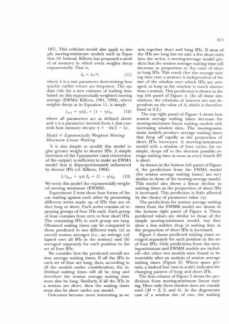
107). This criticism would also apply to sim­ple moving-minimum models such as Equa­tion 10. Instead, Killeen has proposed a mod­el of m emory in which event weights decay exponentially. That is ,

( 11)

where A is a rate parameter determining how quickly earlier events are forgotten. The up­date rule for a new es timate of waiting time based on this exponentially weighted moving average (EWMA: Killeen, 1981, 1994), where weights decay as in Equation 11 , is simply

t.V+ 1 = -yAI\' + (1 - -y) tN> (12)

where all parameters are as defined above and -y is a parameter derived from A that con­trols how memory decays: -y = - In (1 - A) .

Model 4: Exponentially Weighted Moving­lvIinimum Linear Waiting

It is also simple to modify this model to give greater weight to shorter IFIs. A simple inve rsion of the I parameter (and reinversion of the output) is sufficient to make an EWMA model that is disproportionately influenced by shorter IFIs (cf. Killeen, 1984):

1/ tN+ 1 =-yA//,y + (1 - -y)tN' (13)

We term this model the exponentially weight­ed moving minimum (EWMM).

Experiment 2 tests these four forms of lin­ear waiting against each other by presenting different series made up of IFIs that are e i­ther long or short. Each series consists of re­peating groups of four IFIs each. Each group of four contains from zero to four short IFIs. The remaining IFIs in each group are long. Obtained waiting times can be compared to those predicted in two different ways: (a) as overall session averages (i.e., an average col­lapsed over all IFIs in the session) and (b) averaged separately for each position in the set of four IFIs.

We consider first the predicted overall ses­sion average waiting times. If all the IFIs in each set of four are long, then, according to all the models under consideration, the in­dividual waiting times will all be long and therefore the session average waiting time must also be long. Similarly, if all the IFIs in a session are short, then the waiting times must also be short under any model.

Outcomes become more interesting as we

611

mix together short and long IFIs. If most of the IFIs are long but we mix a few short ones into the series, a moving-average model pre­dicts that the session average waiting time will decrease in proportion to the ratio of short to long IFIs. This result (for the average wait­ing time over a session) is independent of the size of the window over which IFIs are aver­aged, as long as the window is much shorter than a session. This prediction is shown in the top left panel of Figure 4. (In all these sim­ulations, the relations of interest are not de­pendent on the value of A, which is therefore fixed at 0.2.)

The top right panel of Figure 4 shows how session average waiting times d ecrease for moving-minimum linear waiting models with increasing window sizes. The moving-mini­mum models produce average waiting times that drop off rapidly as the proportion of short IFIs increases. A moving-minimum model with a window of four cycles, for ex­ample, drops off to the shortest possible av­erage waiting time as soon as every fourth IFI is short.

As shown in the bottom left panel of Figure 4, the predictions from the EWMA model (for session average waiting times) are very similar to those of the moving-average mode l. This model also shows a linear d ecline in waiting times as the proportion of short IFIs is increased. This prediction is little affected by the choice of parameter value (-y).

The predictions for session average waiting times from the EWMM model are shown in the bottom right panel of Figure 4. These predicted values are similar to those of the simple moving-minimum model , but they show a less sudden drop in waiting time as the proportion of short IFIs is increased.

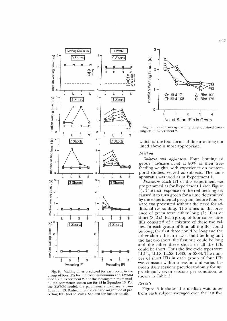
Figure 5 shows predicted waiting times av­eraged separately for each position in the set of four IFIs. Only predictions from the mov­ing-minimum and EWMM models are includ­ed-the other two models were found to be nonviable after an analysis of session average waiting times (Figure 6). Where space per­mits, a dashed line (not to scale) indicates th e changing p attern of long and short IFIs.

The first column of Figure 5 shows the pre­dictions from moving-minimum linear wait­ing. Here only three window sizes are consid­ered (M = 2, 3, and 4). In the degenerate case of a window size of one, the waiting

612

3 IMoving Average I 3

IMoving Minimuml -(J) -- -<r 1 -fro 2

(j)

E 2 '';:;

-a- 3 -¢- 4

2

0> C

'';:;

'co 3 c .~ "0 (j)

E

0 o~~----~--~----~--~--

3 3 EWMA EWMM -(J) --

Qj E 2

'';:;

0> C

,' .

•••• ,' . .... -<r 0.1 -Is- 0.3 -a- 0.5 -¢- 0.7 -+ 0.9

-<r 0.1 -fro 0.3 -a- 0.5 -¢- 0.7 + 0.9

2

'';::;

'co ..... ~

3 c <U

~ E ".:"

0 O~~----r---~--~----'--

o 1 234 o 1 2 3 4

No. of Short IFls in Group No. of Short IFls in Group

Fig. 4. Session average waiting times predicted by four models in Experiment 2. Top left panel: predictions from moving-average linear waiting. Top right panel: predictions from moving-minimum linear waiting. Pal'ameter values shown are for M in Equation 10. Bottom left panel: predictions from the EWMA model. Parameter values are for "I in Equation 12. Bottom right panel: predictions from the EWMM model. Parameter values al'e for "I in Equation 13. See text for further details of models.

times would track IFIs perfectly. Window sizes greater than four behave the same as for a window size of four (squares in Figure 5)­no change in waiting time through the groups of four IFIs.

For moving-minimum linear waiting, wait­ing times track the series of IFIs; but rather than tracking smoothly, the model is more in­fluenced by short IFIs than by long ones, and therefore drops off rapidly to shorter waiting times. Consider for example the condition in which M = 3. If any of the last three IFIs is short, then a short waiting time is emitted. Only if all three of the last IFIs are long is a long waiting time predicted. Thus only in the

one-short condition is any tracking observed at this parameter value.

For the EWMM model, values of'Y deter­mine the responsiveness of the model, but in general there is a progressive increase in wait­ing times for each successive long IFI and a progressive decrease for each short IF!. Sim­ilarly to the moving-minimum model, the be­havior of this model is asymmetrical; each successive long IFI causes a gradual increase in waiting time, whereas a single short IFI causes a precipitous drop in waiting time.

Experiment 2 exposed pigeons to series of IFIs containing from zero to four short IFIs in every group of four IFIs, in order to test

I Moving Minimum I EWMM

:0;3 10 ShOrtsl 3 10 Shortsl

a.; .§ 2 ~ 2 I! " " I! OJ -0-2 . .§ -tr- 3 0----0--0--0 '(1; -0- 4 -0- 0.1 !: 1 -tr- 0.3

-0- 0.5 c ________ ± .0. 7 ell -----------'6 Q)

-+- 0.9

E 0 -,- 0 L L L L L L L L

~3 11 Shortl 3 11 Short I

a.; .§ 2

!l\ 2

OJ c :-= ~ 1 c ell

0-----0-0------'6 Q)

E 0 0 L L L S L L L S

:0;3 12 Shorts I 3 12 Shortsl iii .§ 2 2

~ OJ c

:-2 ell :: 1 c ell '6 Q)

E 0 0 L L S S L L S S

~3 13 Shortsl 3 13 Shortsl

a.; .§ 2 2 OJ c

L :-2 ell :: 1 c ell

!t---O---O---fl '6 Q)

E 0 0 L S S S L S S S

:0;3 14 ShOrtsl 3 14 ShOrtsl

a.; .§ 2 2 OJ c :.a ~ 1 c ell

!t---O---O---fl • • • • '6 Q)

E 0 0 S S S S S S S S

Preceding IFI Preceding IFI

Fig. 5. Waiting times predicted for each point in the group of four IFIs for the moving-minimum and EWMM models in Experiment 2. For the moving-minimum mod­el, the parameters shown are for M in Equation 10. For the EWMM model, the parameters shown are 'Y from Equation 13. Dashed lines indicate the magnitude of pre­ceding IFIs (not to scale). See text for further details.

3

-en --a; E 2 -0> c: -'co ~ c: co :0 (j)

E

~ Bird 17 -0- Bird 105

-!:s- Bird 102 -¢- Bird 175

O~-r---'----T----r--~--

o 1 234

No. of Short IFls in Group

Fig. 6. Session average waiting times obtained h'om -l subjects in Exper'iment 2.

which of the four forms of linear waiting out­lined above is most appropriate.

Method

Subjects and apparatus. Four homing pi­geons (Columba Livia) at 80% of their fre e­feeding weights, with experience on nontem­poral studies, served as subjects. The same apparatus was used as in Experiment 1.

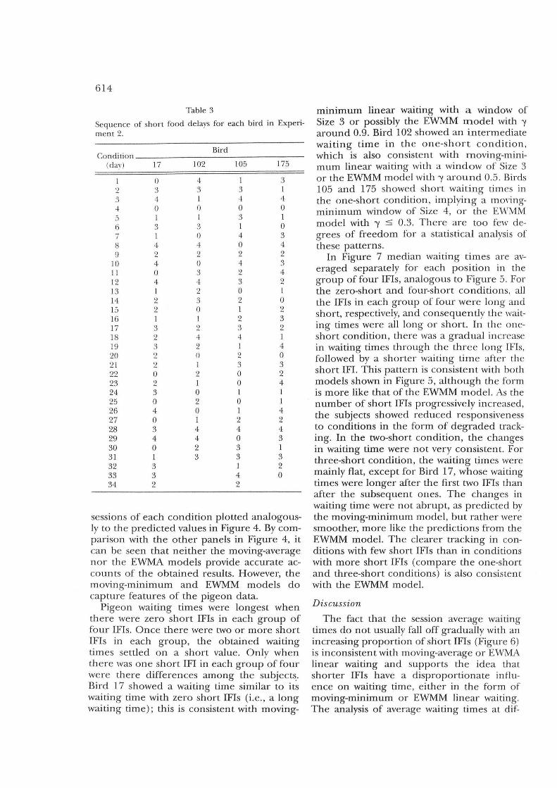
Procedure. Each IFI of this experiment was programmed as for Experiment 1 (see Figure 1). The first response on the red pecking key caused it to turn green for a time determined by the experimental program, before food re­ward was presented without the need for ad­ditional responding. The times in the pres­ence of green were either long (L; 10 s) or short (S; 2 s). Each group of four consecutive IFls consisted of a mixture of these two val­ues. In each group of four, all the IFIs could be long; the first three could be long and the other short; the first two could be long and the last two short; the first one could be long and the other three short; or all the IFIs could be short. Thus the five cycle types were LLLL, LLLS, LLSS, LSSS, or SSSS. The num­ber of short IFIs in each group of four IFIs was constant within a session and varied be­tween daily sessions pseudorandomly for ap­proximately seven sessions per condition , as shown in Table 3.

Results Figure 6 includes the median wait times

from each subject averaged over the last five

614

Table 3

Seq uence of sho n food delays for each bird in Experi-ment 2.

Conditio n Bird

(dav ) 17 102 105 175

0 4 1 3 ':2 :3 3 3 1 3 4 1 -! 4 ..j. 0 0 0 0 5 I 1 3 1 [i 3 3 1 0 7 0 4 3 8 4 4 0 4 C) 2 2 2 2

10 4 0 4 3 11 0 3 2 4 12 4 4 3 2 13 1 2 0 1 14 2 3 2 0 15 2 0 I 2 16 I 2 3 17 3 2 3 2 18 2 ..j. 4 1 19 3 2 I 4 20 2 0 2 0 2 1 ':2 3 3 22 0 2 0 2 23 2 I 0 4 24 3 0 1 1 25 0 2 0 1 26 4 0 I 4 27 0 I 2 2 28 3 4 4 4 29 4 4 0 3 30 0 2 3 1 31 1 3 3 3 32 3 I 2 33 3 4 0 34 2 2

sessions of each condition plotted analogous­ly to the predicted values in Figure 4. By com­parison with the other panels in Figure 4, it can be seen that neither the moving-average no r the EWMA models provide accurate ac­counts of the obtained results. However, the moving-minimum and EWMM models do capture features of the pigeon da ta.

Pigeon waiting times were longest when th ere were zero short IFls in each group of four IFls. Once there were two or more short IFls in each group, the obtained waiting times settled on a short value. Only when th e re was one short IFI in each group of four were th ere differences among the subject~. Bird 17 showed a waiting time similar to its waiting time with zero short IFls (i.e., a long waiting time); this is consistent with moving-

mInImUm linear waItIng with a window of Size 3 or possibly the EWMM model with 'Y around 0.9. Bird 102 showed an inte rmediate waiting time in the one-short co ndition , which is also consistent with moving-mini­mum linear waiting with a window of Size 3 or the EWMM model with 'Y around 0. 5. Birds 105 and 175 showed short waiting tim es in the one-short condition, implying a moying­minimum window of Size 4, or the Ev\'MM model with 'Y :s 0. 3. There are too few de­grees of freedom for a sta tistica l ana lysis of these pa tterns .

In Figure 7 median waiting times are av­eraged separately for each position in the group of four IFIs, analogous to Figure S. For the zero-short and four-short conditions, all the IFls in each group of four were long and short, respective ly, and consequently the wait­ing times were all long or short. In th e one­short condition, there was a gradual increase in waiting times through th e three long IFIs, followed by a shorte r waiting time after th e short IF!. This pattern is consistent with both models shown in Figure 5, although th e form is more like that of the EWMM model. As the number of short IFIs progressive ly increased, the subjects showed reduced responsiveness to conditions in the form of degraded track­ing. In the two-short condition, the changes in waiting time were not very consistent. For three-short condition , the waiting times were mainly flat, except for Bird 17, whose waiting times were longer after the first two IFIs than after the subsequent ones. The changes in waiting time were not abrupt, as predicted by the moving-minimum model, but rather were smoother, more like the pre dictions from the EWMM model. The clearer tracking in con­ditions with few short IFIs than in conditions with more short IFIs (compare the one-short and three-short conditions) is also consistent with the EWMM model.

Discussion

The fact that the session average wanmg times do not usually fall off gradually with an increasing proportion of snort IFIs (Figure 6) is inconsistent with moving-average or EWMA linear waiting and supports th e idea that shorter IFIs have a disproportionate influ­ence on waiting tim e, either in the form of moving-minimum or EWMM linea r waiting. The analysis of average waiting times at dif-

-3 $

Qi

.~ 2 C> c:

'';::;

.~

c: ell

~

~ Bird 17 -lr Bird 102 v Bird 105 -<>- Bird 175

E 0 ~"""--r---r----'--

-3 $

<I>

. ~ 2 C> c: -.~ c: ell

~

L L

E O~-r---r----'--~-

-3 $

Qi

.~ 2 C> c:

'';::;

.~

c: ell

~

L L L s

12 Shorts!

----- 1 1 ____ _

E 0 ~-,---,---,---,--

-3 $

Qi

.S 2 -C> c:

'';::;

.~

c: ell

~

L L s s

13 Shorts!

E 0 ~-,--.,....-.,....-.,....-

-3 $

Qi

.~ 2 C> c: -. ~ c: ell

~

L s s s

14 Shorts!

E 0 ~-,--.,....--,---,--s s s s

Preceding IFI

615

ferent positions in the four IFI groups (Fig­ure 7) supported the EWMM but not the moving-minimum model. Both analyses suggest that for most subjects, values of"{ less than 0.5 are most appropriate; this value in­dicates that the immediately preceding IFI contributes less than 50% to the next waiting time (the remaining control comes from ear­lier IFls in an exponentially d ecaying series) . The exception was Bird 17, which appears to have had a significantly larger value for ,,{ , im­plying that the immediately preceding IFI was the main controlling factor for the present waiting time .

GENERAL DISCUSSION

These experiments show that pigeons are able to react rapidly to changes in temporal patterning of food delivery (at least at the short IFIs used here). It appears for our pi­geons that waiting times were predominantly controlled not by the immediately preceding IFI, but by an average of the last few IFIs, where the calculation of that average is dis­proportionately influenced by shorter IFI val­ues, and by more recent IFIs. A model imple­menting these features (the EWMM model, Equation 12) best accounted for the results of Experiment 2.

Experiment 1 demonstrated that pigeons can track different series of rapidly changing IFls that vary randomly from day to day. How­ever, their ability to track was degraded by noise added to the series of IFls: The greater the noise, the poorer the tracking. This deg­radation implies that waiting time is affected by IFls earlier than the immediately preced­ing one.

Experiment 2 tested four different forms of linear waiting that, in different ways, allowed IFIs earlier than one back to influence wait­ing time. The manner in which waiting times changed as differen t patterns of long and short IFls were presented was inconsistent with models that assumed that an arithmetic mean moving average of the last few IFls was

Fig. 7. Obtained median waiting times for each bird in Experiment 2 averaged separate ly for each position in the group of four !FIs. Dashed lines indicate the magni­tude of the preceding IFI (not to scale).

616

controlling waiting time. Models that give a disproportionate weight to shorter IFIs were, however, consistent with these results. The best descriptor of the obtained results was the EWMM model, which is based on an expo­nentially weighted moving average of the in­verted IFI values. By inverting the IFI value (and then reinverting the output of the mod­el) , smaller IFI values come to have a dispro­portionate influence.

A version of linear waiting, such as EWMM, that gives a disproportionate weight to short­er IFIs can account for a wide range of ap­parently inconsistent phenomena in the lit­erature on the dynamics of adaptation to time. In the introduction we described our autocatalytic schedule (Wynne & Staddon , 1988, Experiment 3). When the multiplier controlling the relationship between waiting time and IFI (w) was small, the waiting times on this schedule reliably and rapidly became very short. When the w values were large , the waiting times tended to increase, as expected from the one-back version of linear waiting, but in general the subjects' responding did not cease. The results from Experiment 2 clarified the reasons for this asymmetry. When the w value was large, the EWMM pro­cess protected the subject against "inflation­ary" increases in waiting time, because any occasional short IFls in the recent past put pressure on waiting times to remain short. Only when all recent IFIs were long was wait­ing time forced to increase. Thus, EWMM lin­ear waiting permits rapid adaptation to tem­poral regularities in the environment but also protects subjects against the excessively long (in the sense that available reinforcers are missed) waiting times that would be pro­duced under certain conditions by one-back or moving-average versions of linear waiting.

Staddon and associates (Innis & Staddon, 1970; Kello & Staddon, 1974; Staddon, 1967, 1969) tested pigeons on a variety of proce­dures in which fixed-interval (FI) schedules of two durations were programmed in re­peating cycles. The general form of these schedules was 12 FI 1 min followed by a FI x­min schedules, where ax = 12. Thus each study consisted of cycles of 12 FI 1 min fol­lowed by a 12-min phase of a longer FI value. In one study the second half of each cycle consisted of six FI 2-min schedules (12 FI 1, 6 FI 2); in another the second half consisted

of four FI 3-min schedules (12 FI 1, 4 FI 3); and in a third the second half consisted of two FI 6-min schedules (12 FI 1, 2 FI 6). In all cases, waiting time during the long IFI part of the schedules differed little from wait­ing time during the short IFI part, even after extended training. Waiting times (postrein­forcement pauses) throughout were close to 30 s, a value typical of the pauses on the FI I-min schedules in the first half of each cvcle. In the second half of each cycle, very slight increases in pause length were observed un­der the FI 2-min condition, and some pauses shorter than 30 s were observed in the FI 6-min intervals. Pausing on the FI 3-min sched­ules was identical to that found under the 12 FI I-min schedules. Although we do not know whether the models developed here apply without modification to the substantiallv lon­ger intervals used in these earlier studies, their results are nonetheless consistent with the present account. The counterintuitive re­sult that pauses on the FI 2-min schedules were longer than those on FI 3-min and FI 6-min schedules is explained by the fact that, in these studies, the number of consecutive presentations of each FI value was inversely proportional to the length of the FI. If the subjects' pauses were determined by the shortest of recent IFIs, then control by the longer FIs can only be expected when enough of them occur consecutively that the EWMM process is no longer assessing any short FIs. When the FI value was 2 min, six presentations of this schedule were made, compared to only two presentations: of the FI 6-min schedule. Thus the EWMM process as­sessed more long IFIs under the FI 2-min condition than under the FI 6-min condition, leading to longer pausing.

Innis (1981, Experiment 3, Condition 1) investigated schedules in which two FI values appeared in double alternation. The general form of these schedules was two FI 28, two FI 68, where 8 took on three values: 5, 15, and 30 s. In every case, waiting times failed to track changing FI values. Innis found a similar lack of temporal control in a condi­tion in which long and short FI values were presented in strict alternation (Innis, 1981, Experiment 4). All of these results are con­sistent with EWMM linear waiting, because there were never sufficient consecutive long

IFI values to break the disproportionate influ­ence of short IFls.

Innis and Staddon (1971; see also Innis, 1981) compared cyclic-interval schedules wi th differen t forms of progressions. In three conditions , pigeons were exposed to a set of seven Fls increasing either from 20 to 80 s and back to 20 s in arithmetic steps; from 18 to 69 s and back in steps forming a logarith­mic series; or in geometric steps from 3 to 176 s and back. Innis and Staddon concluded from visual inspection of the series of aver­aged postreinforcement pauses that the pi­geons were tracking the FI values under all conditions at a lag of zero or one cycle. Track­ing was clearer under the arithmetic and log­arithmic cyclic schedules than under the geo­metric cyclic schedule. This would be expected from models that give a dispropor­tionate weight to shorter IFIs, because the oc­casional long IFIs in a geometric series are ignored by models of this type.

Recently, Higa et al. (1993) trained pigeons on a sequence of IFIs of 15 s that, at an un­predictable point in the session, could change either to IFIs of 5 s (step down) or 45 s (step up). Higa et al. found that the sub­jects responded almost immediately to the step-down change in IFIs, but only gradually to a step-up change. Wynne and Staddon (1992, Experiment 5) found similar results in an analysis of adaptation to longer IFIs. Blocks of sessions in which the food delay on an RID schedule was 40 s alternated with blocks of sessions with food delays of 20 or 80 s. The development of waiting times ap­propriate to the 40-s food delay was much faster after previous experience with delays of 80 s than after delays of 20 s. These results are further evidence that short IFls dominate over long ones in controlling waiting time.

There are some results that, at first glance, do not appear to be easily reconciled with the EWMM model. Higa et al. (1991, Experiment 3) simply presented pigeons with a series of 100 IFls, 99 of which were of 15-s duration. Intercalated in this series was a single, ran­domly placed 5-s IFI "impulse." Three of 4 subjects showed a response to this impulse that consisted of a single shorter waiting time in the immediately following IFI and a return to waiting times consistent with the longer IFI value more or less immediately thereafter. One subject showed an only slightly shorter

3

Qj 2 E -

617

I Higa et aI.' s Impulse Experiment I +0.9 -<r 0.7 -Q- 0.5 -i:r 0.3 -0- 0.1

5 10 post impulse IFI number

Fig. 8. Waiting times predicted from the EWMlv\ model for Higa et al.'s (1991) impulse experiment. The impulse IFI is IFI O. See text for further details.

waiting time in the postimpulse IFI, followed by a gradual return over three or four IFIs to the waiting time produced before the im­pulse. At first glance the evidence from the majority of these subjects appears to support one-back linear waiting and not the EWMM model.

However, the predictions of these models are often nonintuitive, so we performed a simulation of the behavior pre dicted by EWMM linear waiting. Figure 8 shows pre­dicted waiting times from the EWMM model for a range of values of 'Y following a single short (5-5) IFI embedded in a series oflonger (15-s) IFls. Clearly, at higher values of 'Y (> 0.7), the impact of the short IFI on waiting time was almost entirely confined to the first postimpulse IF!. Because in reality, the wait­ing times vary noisily from IFI to IFl, the ap­parent presence of an effect of the impulse on later IFIs for values of'Y around 0.5 to 0.7 would probably not be detectable in empiri­cal data. At values of'Y less than 0.5, the im­pact of a short IFI lasts longer, but it is also much smaller in the first postimpulse IF!. This is precisely the pattern found for the one divergent subject in this experiment. Thus, on closer inspection , the EWMM mod­el can account both for the short-lived but intense response to a single shorter IFI of the majority of subjects and also for the longer lasting, less intense response of the one re­maining subject.

Is there a functional explanation for pi­geons' special sensitivity to short IFls? This sensitivity may be a conservative strategy that

618

reduces the possibility that a subject will miss an opportunity to get food. Mter all, there is an asymmetry in much operant behavior: The cost of making an operant response is usually very small , but the cost of missing an available food delivery is high. Hence, when in doubt, respond. There is also the logical fact that waiting time is defined by the first response in the IF!. .As we have pointed out elsewhere (Higa et al., 1991; Wynne & Staddon, 1992), a small tendency to respond early in an IFI will dominate even a strong tendency to re­spond later, simply because an early response removes the possibilily of producing a longer waiting time (this is the problem with relying exclusively on waiting time as a measure).

In conclusion, the studies reported here have shown that, although adaptation to changing IFIs can be rapid, nonetheless it is not typically one back, as we had originally proposed (Wynne & Staddon, 1988). Rather, a model proposing that the last few IFIs in­fluence waiting time in such a way that short IFIs have a greater influence than longer ones can account for the data from these ex­periments and from a wide range of disparate results in the literature. Further research needs to analyze more closely the manner in which IFIs are combined and the factors that control the size of the window over which IFIs are measured.

REFERENCES

Capehart, G. w., Eckerman, D. A., Guilkey, M., & Shull, R. L. (1980). A comparison of ratio and interval re­inforcement schedules with comparable inter-rein­forcement times. Journal of the Experimental Analysis of Behavior; 34, 61-76.

Ferster, C. B. , & Skinner, B. F. (1957). Schedules of rein­forcement . New York: Appleton-Century-Crofts.

Gibbon,j. (1977) . Scalar expectancy theory and Weber 's law in animal timing. Psychological Review, 84, 279-325.

Higa, j. j., T haw, j. M. , & Staddon, j. E. R. (1993). Pi­geons' wait-time responses to transitions in interfood­interval duration: Another look at cyclic schedule per­formance . Journal oj the Experimental Analysis of Behavior; 59, 529-541.

Higa,j.j. , Wynne , C. D. L., & Staddon,j. E. R. (1991) . Dynamics of time discrimination. Journal of Experimen­tal Psychology: Animal Behavior Processes, 17, 281-291.

Innis, N. 1<.. (1981). Reinforcement as input: Temporal tracking on cyclic-interval schedules. In M. Commons & J A. Nevin (Eds.), Qy,antitative studies of operant be-

havior: Discriminative properties of reinforcement schedule~ (pp. 257-286). New York: Pergamon Press.

Innis, N. 1<.., Mitchell, S. 1<.., & Staddon, J. E. R. (1993). Temporal control on interval sch edules: What deter­mines the postreinforcement pause? Journal of the Ex­perimental Analysis of Behavior; 60, 293-311.

Innis, N. 1<.., & Staddon,J E. R. (1970). Sequential el~ fects in cyclic-interval schedules. Psychonomic Science. 19,313-315.

Innis, N. 1<.., & Staddon, j. E. R. (1971). Temporal track­ing on cyclic-interval reinforcement schedules. Jaurnal of the Experimental Analysis of Behavior, 16, 411-423.

Kello, j., & Staddon, j. E. R. (1974). Contro l of long­interval performance on mixed cyclic-interval sc hed· ules. Bulletin of the Psychonomic Society, 4, 1-4.

Killeen, P. (1981). Averaging theory. In C. M. Bradshaw, F. Szabadi, & C. F. Lowe (Eds.), Qy,antification of steady· state operant behaviour (pp . 21-34). Amsterdam: Elsev­ier I North Holland Biomedical Press.

Killeen, P. R. (1984). Incentive theory III: Adaptive clocks. In j. Gibbon & L. Allen (Eds.), Timing and tin!/! perception. Annals of the New York Academy of Sciences. 423, 515-527.

Killeen, P. R. (1994). Mathematical principles of rein­forcement. Behavioral and Brain Sciences, 17, 105- 172.

Pavlov, I. P. (1928) . Lectures on conditioned reflexes. (W. H. Gantt, Trans.) New York: International Publishers.

Richelle, M., & Lejeune, H. (1980). Time in animal be­haviaur. Oxford: Pergamon Press.

Schneider, B. A. (1969) . A two state analysis of fixed­interval responding in the pigeon. Journal of the Ex· perimental Analysis of Behavior; 12, 677-687.

Shull , R. L. (1970) . The response-reinforcement depen­dency in fixed-interval schedules of reinforcement. Jaurnal of the Experimental Analysis of Behavior, 14, 55-60.

Skinner, B. F. (1938) . The behavior of organisms. New York: Appleton-Century-Crofts.

Staddon, J. E. R. (1965) . Some properties of spaced re­sponding in pigeons. Journal of the Experimental Analysis of Behavior; 8, 19-27.

Staddon, j. E. R. (1967). Attention and temporal dis­crimination: Factors controlling responding under a cyclic-interval schedule. Journal of the Experimental Analysis of Behavior; 10, 349-359.

Staddon, j. E. R. (1969). Multiple fixed-interval sched­ules: Transient contrast and temporal inhibition. Jaur­nal of the Experimental Analysis of Behavior; 12, 585-590.

Staddon,j. E. R., Wynne, C. D. L., & Higa,j.j. (1991). The role of timing in reinforcement schedule perfor­mance. Learning and Motivation, 22, 200-225.

Wynne, C. D. L., & Staddon, j. E. R. (1988). Typical interfood interval determines waiting time on peri­odic-food schedules: Static and dynamic tests. Journal of the Experimental Analysis of Behavior; 50, 197-210.

Wynne, C. D. L., & Staddon,j. E. R. (1992) . Waiting in pigeons: The effects of daily intercalation on tempo­ral discrimination. Jaurnal of the Experimental Analysis of Behavior; 58, 47-66.