xp agenda video last class excel tutorial 3: developing a professional- looking worksheet excel...

XPAgenda

• Video• Last Class• Excel Tutorial 3: Developing a Professional-

Looking Worksheet• Excel Tutorial 4: Working with Charts and

Graphics• Agenda for Next Class

1New Perspectives on Microsoft Office Excel 2003 Tutorial 3

Presentation by: Joseph H. Schuessler, B.B.A., M.B.A., M.S., Ph.D. (ABD)

XPLast Class

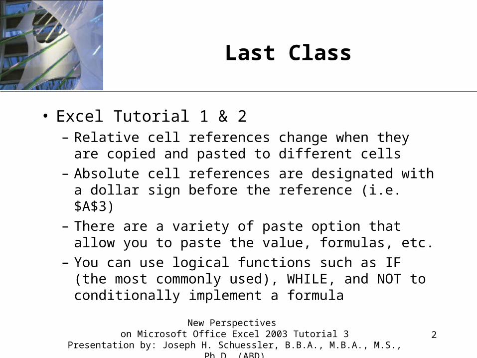
• Excel Tutorial 1 & 2– Relative cell references change when they are copied

and pasted to different cells

– Absolute cell references are designated with a dollar sign before the reference (i.e. $A$3)

– There are a variety of paste option that allow you to paste the value, formulas, etc.

– You can use logical functions such as IF (the most commonly used), WHILE, and NOT to conditionally implement a formula

2New Perspectives

on Microsoft Office Excel 2003 Tutorial 3Presentation by: Joseph H. Schuessler, B.B.A., M.B.A., M.S., Ph.D. (ABD)

XP

3

Microsoft Office Excel 2003

Tutorial 3 – Developing a Professional-Looking Worksheet

New Perspectives on Microsoft Office Excel 2003 Tutorial 3


XP

4

Open the Format Cells dialog box

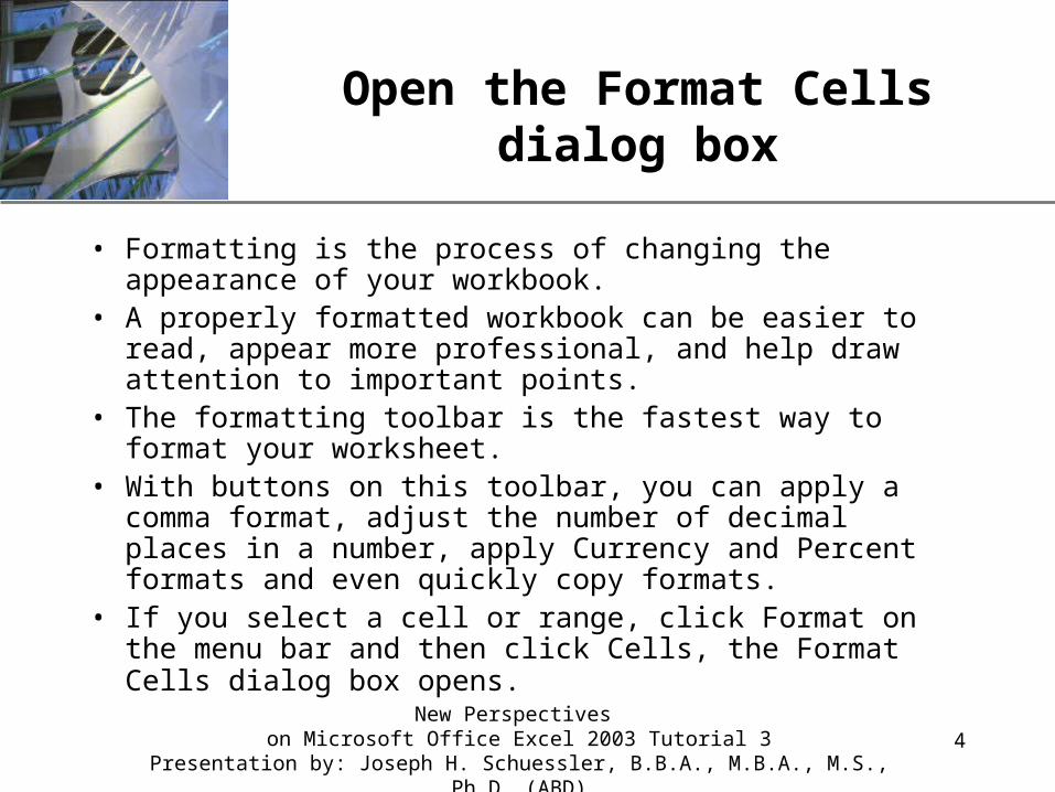
• Formatting is the process of changing the appearance of your workbook.

• A properly formatted workbook can be easier to read, appear more professional, and help draw attention to important points.

• The formatting toolbar is the fastest way to format your worksheet.

• With buttons on this toolbar, you can apply a comma format, adjust the number of decimal places in a number, apply Currency and Percent formats and even quickly copy formats.

• If you select a cell or range, click Format on the menu bar and then click Cells, the Format Cells dialog box opens.



XP

5

The Format Cells dialog box



XP

6

Format data using different fonts, sizes and font styles

• A font is the design applied to letters, characters and punctuation marks. Each font is identified by a font name or type face.

• Fonts can be displayed in various sizes and you can even change the color of the font or the background color in the cell.

• These options are available in the Format Cells dialog box and there are also buttons available for the formatting toolbar to make formatting faster.



XP

7

Align cell contents

• When you enter numbers and formulas into a cell, Excel automatically aligns them with the cell's right edge and bottom border, while text entries are aligned with the left edge and bottom border.

• You can control the alignment of data within a cell horizontally and vertically.

• Left, Right and Center alignments can be selected using their respective alignment buttons on the Formatting toolbar.

• To align the cell's contents vertically, open the Format Cells dialog box and choose the vertical alignment options on the Alignment tab.



XP

8

Align using Merge and Center

• Another option available for alignment in the Format Cells dialog box and on the Format toolbar is the Merge and Center option, which centers text in one cell across a range of cells.

• If you want to fit a lot of text within a cell but without having to expand the column width to be very large, you can use the text wrapping option on the Alignment tab, or even choose to indent text.

• You can also have Excel shrink the text to fit within the given column width you have chosen or even rotate text from -90 to +90 degrees.



XP

9

The Alignment tab of the Format Cells dialog box



XP

10

Examples of text formatting



XP

11

Add cell borders and backgrounds

• Excel provides a range of tools to format not only the contents of a cell, but also the cells themselves.

• The gridlines you see in Excel in a new worksheet are not displayed on printed pages.

• You can add a border to a cell using either the Borders button on the Formatting toolbar or the options on the Border tab in the Format Cells dialog box.



XP

12

The Borders button versus the Border tab

• When you click the list arrow for the Borders button, a Borders palette appears showing common choices as well as a Draw Borders button at the bottom of the Border palette gallery.

• The Borders button allows you to create borders very quickly, whereas the Format Cells dialog box allows you to refine your choices further.

• The Border Tab in the Format Cells dialog box is especially useful for controlling how a block of cells or a range appears with borders.

• You have the option to change the outermost top, bottom and sides of the range independently, as well as determine different borders for the lines separating the cells inside the range's grid.



XP

13

The Border tab of the Format Cells dialog box



XP

14

Add patterns or colors to cells

• Patterns and colors can be used to enhance the appearance of spreadsheet cells.

• The fastest way to apply background color to cells in the worksheet is by clicking the list arrow of the Fill color button and choosing a color from the palette.

• To apply a fill pattern to cells, use the Patterns tab on the Format Cells dialog box.



XP

15

The Patterns tab of the Format Cells dialog box



XP

16

A worksheet with formatting applied



XP

17

Merge a range of cells

• To merge a range of cells into a single cell:– Use the Merge option on the Alignment tab in the

Format Cells dialog box– Click the Merge and Center button on the Formatting

toolbar

• To split a merged cell back into individual cells:– Select the merged cell – Click the Merge and Center button again– Or uncheck the Merge Cells check box on the

Alignment tab in the Format Cells dialog box New Perspectives

on Microsoft Office Excel 2003 Tutorial 3Presentation by: Joseph H. Schuessler, B.B.A., M.B.A., M.S., Ph.D. (ABD)

XP

18

Merge headings across multiple cells



XP

19

Hide rows and/or columns

• You can hide rows or columns, which does not affect the data stored there, nor does it affect any cell that might have a formula reference to a cell within the hidden row or column.

• To hide a row or column:– Select the row or column and then choose Hide from either the

Row or Column option of the Format menu, or, from the shortcut menu that pops up when you right click the row or column heading

• To unhide a row or column:– Select the headings of the rows or columns that border the hidden

area, then choose Unhide from either the Row or Column option of the Format menu, or, from the shortcut menu that pops up when you right click the row or column heading



XP

20

Worksheet with hidden cells



XP

21

Format the worksheet background and sheet tabs

• You can use an image file as a background for a worksheet.

• Images can be used to give the background a textured appearance, like that of granite, wood, or fibered paper.

• The background image does not affect the format or content of any cell in the worksheet, and if you have already defined a background color for a cell, Excel displays the color on top, hiding that portion of the image.

• You cannot apply a background image to all the sheets of the workbook at the same time.



XP

22

Insert a background image and change a worksheet tab color

• To add a background image to a worksheet:– Click Format on the menu bar, point to Sheet and click

Background – Locate and select an image from your hard drive, floppy drive,

network, etc., and click the Insert button • You can also format the background color of the

worksheet tabs, but this color is only visible when the worksheet is not the active sheet in the workbook. – Right click the tab you want to change and choose Tab color from

the shortcut menu – Select a color from the color palette, click the OK button, and then

click on a different tab in order to see the color displayed on the changed tab



XP

23

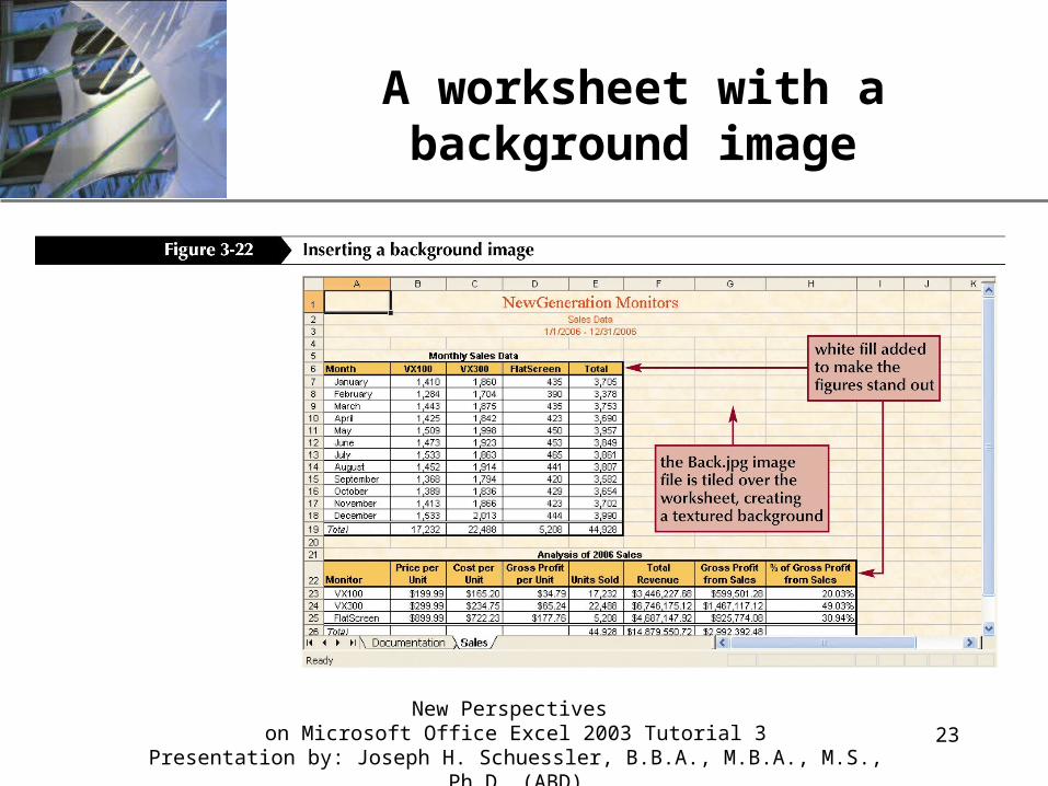
A worksheet with a background image



XP

24

Find and replace formats within a worksheet

• The Undo button on the Standard toolbar is very useful for removing formatting choices you have decided you do not want to use.

• You can also clear the formatting of selected cells, returning them to their initial, unformatted appearance. – To clear formatting, select a cell or range, click Edit on

the menu bar, point to Clear and then click Formats



XP

25

Use Find and Replace to change formats

• Click Edit on the menu bar and then click Replace. • When the Find and Replace dialog box opens, click the

Options >> button to expand the box and display additional find and replace options.

• Click on the Replace tab and then click the topmost Format button to open a Find Format dialog box, select the format combinations you want to search for, then click the OK button.

• Click the lower Format button and when the dialog box opens, select the options you want to use for replacing the formatting.

• Click the OK button and then the Replace All button to quickly change all the cells that meet your Find Format criteria.

XP

26

Dialog boxes used for Find and Replace operations



XP

27

Create and apply styles

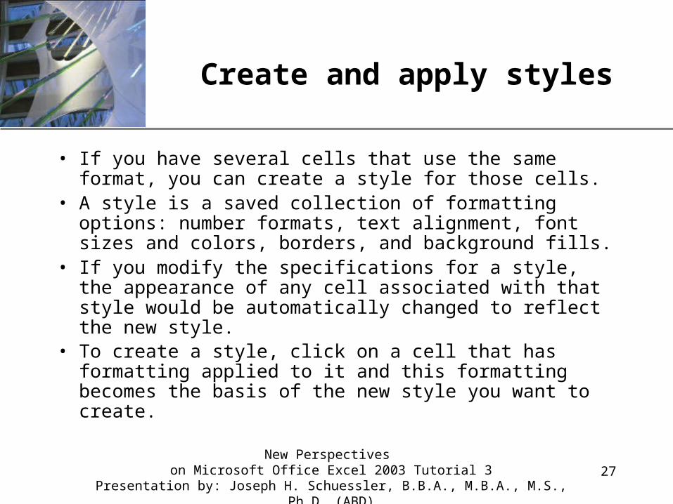
• If you have several cells that use the same format, you can create a style for those cells.

• A style is a saved collection of formatting options: number formats, text alignment, font sizes and colors, borders, and background fills.

• If you modify the specifications for a style, the appearance of any cell associated with that style would be automatically changed to reflect the new style.

• To create a style, click on a cell that has formatting applied to it and this formatting becomes the basis of the new style you want to create.



XP

28

Create a style using the Style dialog box

• Click Format on the menu bar, and then click Style. The Style dialog box opens and all the formatting options associated with the active cell are listed.

• Give the style a name, and then modify the formatting options by removing or adding to the existing ones listed in the dialog box. Click the OK button to create a style with a specific name.

• To apply a style within a worksheet, first select the cells you want associated with the style, then open the Style dialog box, choose the style name from the list arrow and then click the OK button.

• When you create a style, you can also click the Merge button in the Style dialog box to merge a style with those from other open workbooks.



XP

29

The Style dialog box



XP

30

Apply an AutoFormat to a table

• You can apply a professionally designed format to your worksheet by choosing one of 17 predefined formats from the AutoFormat gallery.

• To apply an AutoFormat to a table:– Select a range that has a table of information in it – Click Format on the menu bar, click AutoFormat and the

AutoFormat dialog box opens. Scroll through the gallery to view different table formats, click on one you want to try, and then click the OK button.

– Click on a cell outside of your selected range to remove the highlighting from your table so you can see what it looks like with the AutoFormat design applied.



XP

31

The AutoFormat style gallery



XP

32

Format a printout using Print Preview

• Open a Print Preview window by clicking the Print Preview button on the Standard toolbar.

• Excel will display the preview as a full page, which may be difficult to read.

• Click the Zoom button on the Print Preview toolbar, or pass your mouse over the page, and the pointer changes to the shape of a magnifying glass. When you click any portion of the page Excel will zoom in. Zoom out using the same methods.

• By clicking the Setup button on the Print Preview toolbar, you can change margins, orientation, center the page or set several other formatting and printing features.

• You can also open the Page Setup dialog box by selecting that option from the File menu.



XP

33

The Margins tab of the Page Setup dialog box



XP

34

Create a header and footer for a printed worksheet

• A header is text printed within the top margin of every worksheet page and a footer is printed within the bottom margin of every page.

• Headers and footers can add important information to your printouts.

• Excel tries to anticipate headers and footers and provides several preformatted options in list boxes on the Header/Footer tab of the Page Setup dialog box.

• Click the list arrow for these header and footer options and select one of Excel's suggestions or create your own by choosing the Custom Header or Custom Footer buttons on the Header/Footer tab.



XP

35

The Header dialog box



XP

36

Define a print area and add a page break to a printed worksheet

• By default, Excel prints all parts of the active worksheet that contain text, formulas, or values.

• You can define a print area that contains only the content that you want to print.

• To define a print area, select the range you want to print, click File on the menu bar, point to Print Area, and then click Set Print Area.

• You can also specify different sections of your worksheet to print on separate pages. – Insert a page break by clicking on a cell, clicking Insert on the

menu bar, and then clicking Page Break



XP

37

The Sheet tab of the Page Setup dialog box



XP

38

Microsoft Office Excel 2003

Tutorial 4 – Working With Charts and Graphics



XP

39

Create column and pie charts in Excel

• Charts, or graphs, provide visual representations of the workbook data.

• A chart may be embedded in an existing worksheet, or can be created on a separate chart sheet, with its own tab in the workbook.

• You can use Excel’s Chart Wizard to quickly and easily create charts.

• The Chart Wizard is a series of dialog boxes that prompt you for information about the chart you want to generate



XP

40

Create a chart usingthe Chart Wizard

• To create a chart with the Chart Wizard:– Select the data you want to chart, which will be your data source

– Click the Chart Wizard button on the standard toolbar

– In the first step of the chart wizard, select the chart type and sub-type

– In the second step of the Chart Wizard, make any additions or modifications to the chart's data source

– In the third step, make any modifications to the chart's appearance

– In the fourth and final step, specify the location for the chart, then click the OK button



XP

41

Chart Wizard dialog box 1



XP

42

Choosing a data series

• You can alter the data source during step 2 of the Chart Wizard and also choose whether to organize the data source by rows or by columns.

• The data source is organized into a collection of data series. – A data series consists of data values, which are plotted on the

chart's vertical, or Y-axis – The data series’ category values, or X values, are on the horizontal

axis, called the X-axis

• A chart can have several data series all plotted against a common set of category values.



XP

43




XP

44

Modify the appearance of a chart

• The plot area contains data markers, examples of which include the columns of a column chart, pie slices in a pie chart, or the points used in an XY (scatter) chart.

• An axis covers a range of values, called a scale. • The scale is displayed by placing values alongside the

axes. • A chart may also contain gridlines by extending the tick

marks into the plot area. • Whenever there are several data series for a chart, a legend

can be placed next to the plot area to uniquely identify each series with a different color or pattern.



XP

45




XP

46




XP

47

Resize and move an embedded chart

• An embedded chart is an object that you can move, resize or copy.

• Select the embedded chart to make it active; the selection handles will appear. To resize the chart:– Drag the selection handles to increase or decrease the size of the

chart – To keep the chart proportions the same as you resize, hold the

Shift key as you drag one of the selection handles – To move the chart, make it active and then move the pointer over a

blank area. Click and drag the embedded chart to the new location and release the mouse button



XP

48

Moving and resizing tips

• When you select the chart to make it active, be sure you have clicked the entire chart, and not just one of its elements. – You will be able to tell by the selection handles, which will appear

at the outermost edges of the chart• When you move the pointer over a blank area of the chart

after you have selected it, you should see the label Chart Area appear.

• These tips will help you select and move the entire chart, and not just one of its elements.



XP

49

A selected embedded chart



XP

50

Create a chart sheet

• Create a chart sheet by using the two options in the fourth step of the Chart Wizard:– One option lets you place the new chart as an object in

any existing sheet, which you can select from a drop down list box

– The other option is to place the chart as a new sheet, which is called a chart sheet

• When you select this option, the chart will appear in a new worksheet with its own tab in the workbook.



XP

51

Create a pie chart

• Pie charts are very useful for comparing values in a data series to each other, but can only use one data series at a time.

• One feature of a pie chart is called exploding, in which you can slightly separate a particular pie slice from the other slices.

• You can explode any or all of the slices of the pie. This is referred to as an exploded pie chart.

• Exploding a pie chart adds emphasis to a particular area of the chart and makes it easier to notice.



XP

52

Explode a pie chart

• You can explode all of the slices by selecting the entire pie itself so that all the individual pieces have selection handles.

• As you click and drag any portion, all the slices of the pie will explode outward from each other.

• When the pie is exploded out to the size you desire, release the mouse button.

• A fully exploded pie chart is also one of the sub-type options of the pie chart type that you will see when you use the Chart Wizard.



XP

53

A pie chart with an exploded slice



XP

54

Modify the properties of your charts

• After you create a chart, you can edit the data that is used in the chart by changing it in the data source worksheet cells.

• If you wanted to remove a data series from all categories, you could delete that particular data series from the worksheet in many cases.

• If you want to remove a slice of a pie chart, you cannot just delete the data in the data source, but rather you must change the cell reference of the data series for the chart.



XP

55

Modify a pie chart

• Make the pie chart active and then click Chart on the menu bar. • Click Source Data. Edit the series in this dialog box, or click the

Collapse Dialog button to temporarily collapse the dialog box so you can drag the pointer over a new range of cells. – Whatever you select will replace the existing range listed in the current

data series you are editing

• You can then expand the dialog box again with the Expand Dialog button, make other changes as desired, and click the OK button.

• To move an embedded chart to a new chart sheet, select the chart, click Chart on the menu bar and click Location. The same dialog box of Step 4 of the Chart Wizard will appear and you can click the option to place the chart as a new sheet and give it a name.



XP

56

Format chart elements

• To format an individual chart element, select the element by clicking it and then format its appearance using the same tools on the Formatting toolbar you used to format worksheet cells.

• You can also double-click the chart element to open a dialog box containing formatting options, or right-click the element and then select the Format command from the shortcut menu to open the dialog box.

• There are three basic types of text in an Excel chart: – Label text – Attached text– Unattached text



XP

57

Excel chart text types

• Label text includes category names, tick mark labels, and legend text, which is linked to or derived from cells in the worksheet.

• Attached text is not linked to any cells in the worksheet; examples include the chart title and the axes titles.

• Unattached text is any additional text that you want to include in the chart.



XP

58

Format colors and patterns

• To work with colors and fills, double-click an element and the Format Data Series dialog box opens.

• You can use options provided on the Patterns tab to change both the border style and the interior of a data marker.

• You can also edit an axis scale by double-clicking any value on an axis to open the Format Axis dialog box.

• In the Format Data Series dialog box, the Pattern tab includes a Fill Effects button that provides a full range of options to create sophisticated colors and patterns, such as gradient, texture or even a picture.



XP

59

The Fill Effects dialog box



XP

60

Add a graphic to a chart

• You can set a graphic image as a background for a chart using options on the Picture tab of the Fill Effects dialog box.

• This can be done for a data marker, but is often more appropriate for a larger portion of the chart itself, such as the plot area.

• You could also place graphics within the data markers, such as the columns in a Column chart.

• The Fill Effects dialog box options for inserting a picture are the same for data markers as they are for other areas of the chart.

• You can choose to stretch the graphic over the entire size of the column, or choose to stack the graphic up to the height of the column.



XP

61

Change the axis scale

• There are four values that comprise the y-axis scale: the minimum, maximum, major unit, and minor unit.

• The minimum and maximum values are the smallest and largest tick marks that will appear on the axis.

• The major unit is the increment between the scale's tick marks.

• The chart has a second set of tick marks, called the minor tick marks, which may or may not be displayed; if shown, their positioning is determined by the minor unit setting.

• Major tick marks are displayed alongside an axis value, whereas minor tick marks, if present, are not alongside an axis value.



XP

62

The Scale tab of the Format Axis dialog box



XP

63

Create 3-D charts

• To create a 3-D chart, you may choose to do so during the first step of the Chart Wizard, as three-dimensional charts are sub-types of most other charts, such as the pie chart.

• To change a chart to a 3-D chart, select the chart, click Chart on the menu bar, and then click Chart Type.

• Choose the 3-D option sub-type of whichever chart type you prefer.

• There are also several 3-D charts on the Custom Types tab of the Chart Type dialog box.



XP

64

Modify 3-D chart options

• A 3-D chart has several options for modifying the 3-D effect. – Perspective is the illusion that parts of the 3-D chart that are farther away

from you decrease in size– Elevation is the illusion that you are looking at the 3-D chart from some

particular height—either above or below the chart – You may also rotate the 3-D chart to bring different parts of the chart to

the forefront • Elevation and rotation are options that you can change with the 3-D

View dialog box, available from the Chart menu.• Excel creates each 3-D chart with a default elevation, rotation and

height. • To change the appearance of a 3-D chart once you have created one,

make sure it is an active chart then click Chart on the menu bar and then click 3-D View.



XP

65

The 3-D View dialog box



XP

66

Insert drawing objects into your workbook

• The Drawing toolbar helps you create many types of graphical shapes.

• Use the Drawing toolbar to add text boxes, lines, block arrows and other objects to charts and worksheets.

• If the Drawing toolbar is not already displayed, choose to display it by clicking View on the menu bar, pointing to Toolbars, and then clicking Drawing.



XP

67

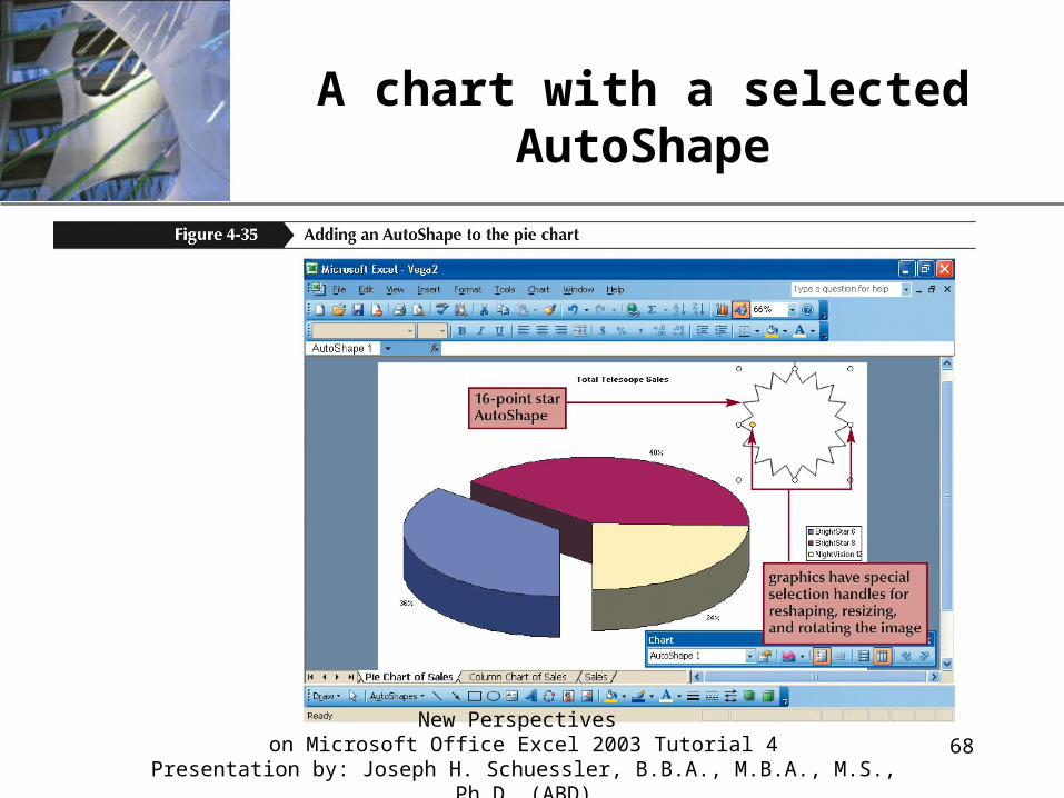
Use Drawing toolbar AutoShapes

• The Drawing toolbar contains a list of predefined shapes, called AutoShapes, which can be anything from simple squares to complicated objects like flow charts or block arrows.

• Once you select a shape from the toolbar, click and drag an area on your chart or worksheet where you want to insert the object and Excel will draw it for you.

• Once you insert a drawing object onto a chart or worksheet, you can resize or move it just like any other object.

• You can also modify the fill color and border style of an AutoShape, and even insert text.



XP

68

A chart with a selected AutoShape



XP

69

Print a chart sheet

• Printing a chart sheet is much the same as printing a worksheet, but in place of the Sheet tab that you would normally see for a worksheet there is a Chart tab. – The Chart tab includes options for Printed chart size and quality

• Excel provides three choices for defining the size of a chart printout: Use full page, Scale to fit page, and Custom.

• As with worksheets, you should preview the printout before sending the chart to the printer.

• You can print multiple sheets at once without printing the entire workbook. Press and hold the Shift key, then click on each sheet you want to print. When finished selecting, release the Shift key and then print.



XP

70

Choose a chart printing option

• When you select the Use full page choice for Printed chart size:– The chart is resized to fit the full page, extending out to the

borders of all four margins, which may change the proportions – This is the default option

• The Scale to fit page choice resizes the chart proportionately until one of the edges reaches a margin border. – When using this choice, the chart may not fit the entire page

• For the Custom choice, dimensions of the printed chart are specified on the chart sheet outside of the Print Preview window.



XP

71

The Chart tab of the Page Setup dialog box



XPNext Class

• Exam I– 90 Multiple guess questions

• 60 from Chapters 1-4

• 30 from Power Point and Front Page

– You’ll have the full class period to complete the exam

– I’ll have the grades posted later that day

72New Perspectives

on Microsoft Office Excel 2003 Tutorials 3 & 4Presentation by: Joseph H. Schuessler, B.B.A., M.B.A., M.S., Ph.D. (ABD)

XPQuestions

73New Perspectives

on Microsoft Office Excel 2003 Tutorials 3 & 4Presentation by: Joseph H. Schuessler, B.B.A., M.B.A., M.S., Ph.D. (ABD)

xp agenda video last class excel tutorial 3: developing a professional- looking worksheet excel...

Documents