y of solar zoa conner - university of tokyo title of dissertation: a stud y of solar neutrinos using...
TRANSCRIPT

Abstract
Title of Dissertation: A STUDY OF SOLAR
NEUTRINOS USING THE
SUPER-KAMIOKANDE DETECTOR
Zoa Conner, Doctor of Philosophy, 1997
Dissertation directed by: Professor Jordan Goodman
Dr. Todd Haines
Department of Physics
The �rst solar neutrino ux results from the Super-Kamiokande detector are de-
scribed. This independent analysis is based on a data set from June 1996 through
February 1997. A total neutrino ux of 2.61 �0:12 (stat) �0:13 (syst) �106 �cm2s
is
implied from the data above a 7 MeV energy threshold. When the measurement
is compared with the most recent Standard Solar Model ux prediction (BP95),
the ratio of data/SSM is 0.394 � 0.018 (stat) � 0.019 (syst). The measured uxes
during day and night yield a fractional di�erence of +0.019 � 0.046 (stat). Inter-
pretations are given in the context of vacuum and MSW enhanced neutrino avor
oscillations.

A STUDY OF SOLAR
NEUTRINOS USING THE
SUPER-KAMIOKANDE DETECTOR
by
Zoa Conner
Dissertation submitted to the Faculty of the Graduate School of theUniversity of Maryland at College Park in partial ful�llment
of the requirements for the degree ofDoctor of Philosophy
1997
Advisory Committee:
Professor Jordan A. Goodman, ChairDr. Todd J. HainesProfessor Elizabeth J. BeiseProfessor David BigioProfessor Rabindra MohapatraProfessor Greg W. Sullivan


Dedication
To my loving parents,
Laurie and Hal Conner
ii

Acknowledgements
This dissertation would not have been possible without the members of the Super-
Kamiokande collaboration. Their hard work went into building, operating, and
understanding the Super-Kamiokande detector.
Graduate school has been a lot of work, but with my wonderful husband, Wal-
ter Roscello, at my side I have had a good time too. His in�nite patience with my
extra long work hours, support and acceptance of my travel schedule (especially
those long trips to Japan), and exceptional love enabled me to excel at my research.
Dr. Todd Haines is a practically perfect mentor for me. He is brilliant, creative,
supportive, and caring. Todd has guided me towards becoming the best researcher
possible and has always been there when I needed him. He has been especially
concerned with helping me maintain a balance between work and my personal life.
Todd is a patient teacher who has given me an unmeasureable amount of advice.
Dr. Jordan Goodman has been supportive in all the ways an advisor should. He
has prodded me to give a variety of international conference talks and high energy
physics seminars. He enthusiastically supports my work to others in the scienti�c
community. Jordan pushes me to always put the physics and the scienti�c facts
before my desire to always be right. He keeps me in touch with both the scienti�c
world and the real world.
I would like to especially thank Dr. Greg Sullivan for becoming an ally so quickly
after joining our group at the University of Maryland and for focussing his e�ort
iii

on the solar neutrino analysis. John Flanagan and Dr. Clark McGrew have been
worthy opponents and strong supporters when working on detector calibration and
simulations. Our spokesmen, Dr. Yoji Totsuka, Dr. Henry Sobel, and Dr. James
Stone, have provided strong support when the senior graduate student on the ex-
periment, me, wanted to represent the Super-Kamiokande collaboration experiment
at international conferences.
Many other people helped or supported in ways too lengthy to list here: Chris
Agrusti, Betty Alexander, Jesse Anderson, Drew Baden, Tomasz Barszczak, John
Cataldi, Mei-Li Chen, Bob Ellsworth, Sarah Eno, Mark Giddings, Nick Hadley,
Hassan Jawahery, Betty Krusberg, Sam Lo and, Adam Lyon, Sara and Eric Mor-
ton, George Parker, Nicholas Phillips, Rob Sanford, Cindy Dion Schwarz, Eric
Sharkey, Andy Stachyra, Juilien Hsu Svoboda, Bob Svoboda, Mark Vagins, Brett
Viren, Camille Vogts, Russell Wood, the rest of the machine shop crew at Mary-
land, and the undergrads processing the data at SUNY.
It is nearly impossible to do research of this type without adequate funding sup-
port. My stipend and tuition for the last six years have been generously provided
by the the National Physical Science Consortium Graduate Fellowship in conjunc-
tion with the National Security Agency and the University of Maryland. My travel
to collaboration meetings, travel to the experiment in Japan, and hardware con-
struction projects have been supported by a subcontract from our collaboration
spokesman, Dr. Henry Sobel. Hank has tried valiantly to make my participation
in the Super-Kamiokande experiment possible. This experiment was made possible
by the cooperation and support from the Kamioka Mining and Smelting Company,
the Japanese Ministry of Science, and the U.S. Department of Energy.
iv

Table of Contents
List of Tables xii
List of Figures xv
1 Introduction 1
1.1 The Sun and the Standard Solar Model : : : : : : : : : : : : : : : : 3
1.1.1 What is the Standard Solar Model? : : : : : : : : : : : : : : 3
1.1.2 How Does the Sun Shine? : : : : : : : : : : : : : : : : : : : 7
1.1.3 Neutrino Spectra and Flux : : : : : : : : : : : : : : : : : : : 7
1.2 The Homestake Experiment : : : : : : : : : : : : : : : : : : : : : : 11
1.3 Kamiokande : : : : : : : : : : : : : : : : : : : : : : : : : : : : : : : 15
1.4 SAGE and GALLEX : : : : : : : : : : : : : : : : : : : : : : : : : : 18
1.5 Current State of the Field : : : : : : : : : : : : : : : : : : : : : : : 20
1.6 Possible Solutions : : : : : : : : : : : : : : : : : : : : : : : : : : : : 22
1.6.1 Reduction of the Central Temperature : : : : : : : : : : : : 22
1.6.2 Smaller Cross Section for 7Be Production : : : : : : : : : : : 23
1.6.3 Low Energy Resonance in 3He + 3He! � + 2 p : : : : : : : 23
1.6.4 Smaller � for �e Capture on 37Cl and 71Ga : : : : : : : : : : 23
1.6.5 Helium Di�usion : : : : : : : : : : : : : : : : : : : : : : : : 24
1.6.6 Neutrino Flavor Oscillations : : : : : : : : : : : : : : : : : : 24
1.6.7 How to Decide Which Solution is Right : : : : : : : : : : : : 30
v

1.7 Sudbury Neutrino Observatory : : : : : : : : : : : : : : : : : : : : 30
1.8 Borexino : : : : : : : : : : : : : : : : : : : : : : : : : : : : : : : : : 32
2 Super-Kamiokande Description 34
2.1 General : : : : : : : : : : : : : : : : : : : : : : : : : : : : : : : : : 34
2.2 Con�guration of the Inner Detector : : : : : : : : : : : : : : : : : : 37
2.3 Con�guration of the Outer Detector : : : : : : : : : : : : : : : : : : 38
2.4 Photomultiplier Tubes : : : : : : : : : : : : : : : : : : : : : : : : : 39
2.5 Electronics and Data Acquisition Systems : : : : : : : : : : : : : : 41
2.5.1 Inner Detector : : : : : : : : : : : : : : : : : : : : : : : : : : 42
2.5.2 Outer Detector : : : : : : : : : : : : : : : : : : : : : : : : : 45
2.6 Triggers : : : : : : : : : : : : : : : : : : : : : : : : : : : : : : : : : 49
2.6.1 Low Energy and High Energy : : : : : : : : : : : : : : : : : 50
2.6.2 Outer Detector : : : : : : : : : : : : : : : : : : : : : : : : : 53
2.6.3 Other Triggers : : : : : : : : : : : : : : : : : : : : : : : : : 54
2.7 O�ine Data Processing : : : : : : : : : : : : : : : : : : : : : : : : : 55
2.8 Water System : : : : : : : : : : : : : : : : : : : : : : : : : : : : : : 56
2.9 Clean Air Systems : : : : : : : : : : : : : : : : : : : : : : : : : : : 56
3 Calibration 59
3.1 Absolute Timing : : : : : : : : : : : : : : : : : : : : : : : : : : : : 59
3.2 Relative Timing : : : : : : : : : : : : : : : : : : : : : : : : : : : : : 60
3.2.1 Light Source : : : : : : : : : : : : : : : : : : : : : : : : : : : 61
3.2.2 Optical Components : : : : : : : : : : : : : : : : : : : : : : 62
3.2.3 Optical Fibers : : : : : : : : : : : : : : : : : : : : : : : : : : 64
3.2.4 Di�users : : : : : : : : : : : : : : : : : : : : : : : : : : : : : 65
3.3 Absolute Energy : : : : : : : : : : : : : : : : : : : : : : : : : : : : 67
vi

3.3.1 Muons : : : : : : : : : : : : : : : : : : : : : : : : : : : : : : 68
3.3.2 �0 Rest Mass : : : : : : : : : : : : : : : : : : : : : : : : : : 69
3.3.3 Decay Electrons : : : : : : : : : : : : : : : : : : : : : : : : : 69
3.3.4 Radioactive Gamma-Ray Sources : : : : : : : : : : : : : : : 69
3.3.5 LINAC : : : : : : : : : : : : : : : : : : : : : : : : : : : : : : 86
3.3.6 Stopped Muon Capture : : : : : : : : : : : : : : : : : : : : : 88
3.4 Detector Monitoring : : : : : : : : : : : : : : : : : : : : : : : : : : 89
4 Simulations 94
4.1 Solar Neutrino Interactions : : : : : : : : : : : : : : : : : : : : : : : 95
4.1.1 Neutrino Energies : : : : : : : : : : : : : : : : : : : : : : : : 95
4.1.2 � � e� Scattering : : : : : : : : : : : : : : : : : : : : : : : 96
4.2 Particle Tracking : : : : : : : : : : : : : : : : : : : : : : : : : : : : 97
4.3 �Cerenkov Light Generation and Tracking : : : : : : : : : : : : : : : 99
4.4 Electronics Simulation : : : : : : : : : : : : : : : : : : : : : : : : : 107
4.5 Trigger Simulation : : : : : : : : : : : : : : : : : : : : : : : : : : : 109
5 Data Reduction - lef1 112
5.1 Introduction : : : : : : : : : : : : : : : : : : : : : : : : : : : : : : : 112
5.2 Goals and Philosophy of lef1 : : : : : : : : : : : : : : : : : : : : : 113
5.3 Event Classi�cation Scheme : : : : : : : : : : : : : : : : : : : : : : 115
5.3.1 Null Trigger Events : : : : : : : : : : : : : : : : : : : : : : : 118
5.3.2 Small Events : : : : : : : : : : : : : : : : : : : : : : : : : : 118
5.3.3 Big Events : : : : : : : : : : : : : : : : : : : : : : : : : : : : 122
5.3.4 Minimum Bias Events : : : : : : : : : : : : : : : : : : : : : 125
5.3.5 Record Keeping : : : : : : : : : : : : : : : : : : : : : : : : : 125
5.4 Hayai Vertex Fitter : : : : : : : : : : : : : : : : : : : : : : : : : : : 125
vii

5.4.1 Algorithm : : : : : : : : : : : : : : : : : : : : : : : : : : : : 127
5.4.2 Performance : : : : : : : : : : : : : : : : : : : : : : : : : : : 129
5.4.3 E�ect of Dwall � 1 meter cut : : : : : : : : : : : : : : : : : : 131
5.5 Track Fitting : : : : : : : : : : : : : : : : : : : : : : : : : : : : : : 134
5.5.1 THR1 : : : : : : : : : : : : : : : : : : : : : : : : : : : : : : 135
5.5.2 THR2 : : : : : : : : : : : : : : : : : : : : : : : : : : : : : : 136
5.5.3 FSTMU : : : : : : : : : : : : : : : : : : : : : : : : : : : : : 137
5.6 Trashman : : : : : : : : : : : : : : : : : : : : : : : : : : : : : : : : 140
5.7 SaveRun : : : : : : : : : : : : : : : : : : : : : : : : : : : : : : : : : 144
5.8 Livetime : : : : : : : : : : : : : : : : : : : : : : : : : : : : : : : : : 147
5.9 E�ciencies : : : : : : : : : : : : : : : : : : : : : : : : : : : : : : : : 148
5.9.1 Muon Identi�cation : : : : : : : : : : : : : : : : : : : : : : : 148
5.9.2 Low Energy Events : : : : : : : : : : : : : : : : : : : : : : : 151
6 Data Reduction - lef2 153
6.1 Introduction : : : : : : : : : : : : : : : : : : : : : : : : : : : : : : : 153
6.2 Good Run/Subrun Selection : : : : : : : : : : : : : : : : : : : : : : 154
6.2.1 lef1 Log Files : : : : : : : : : : : : : : : : : : : : : : : : : 155
6.2.2 Run Log Book : : : : : : : : : : : : : : : : : : : : : : : : : : 160
6.2.3 Run Summary Files : : : : : : : : : : : : : : : : : : : : : : : 161
6.2.4 Decision Making and Record Keeping : : : : : : : : : : : : : 162
6.3 Event Classi�cation Scheme : : : : : : : : : : : : : : : : : : : : : : 162
6.3.1 Pedestal Events : : : : : : : : : : : : : : : : : : : : : : : : 166
6.3.2 Minimum Bias Events : : : : : : : : : : : : : : : : : : : : 166
6.3.3 Caterpillar Muons : : : : : : : : : : : : : : : : : : : : : : : : 168
6.3.4 Big Ringing Events : : : : : : : : : : : : : : : : : : : : : : 169
6.3.5 OD Clipping Muons : : : : : : : : : : : : : : : : : : : : : : 169
viii

6.3.6 Fittable Muon Events : : : : : : : : : : : : : : : : : : : : : 170
6.3.7 LE Ringing Events : : : : : : : : : : : : : : : : : : : : : : 170
6.3.8 LE Junk Events : : : : : : : : : : : : : : : : : : : : : : : : 171
6.3.9 Low Energy Events : : : : : : : : : : : : : : : : : : : : : : : 171
6.4 ComboFit Precision Vertex Fitter : : : : : : : : : : : : : : : : : : : 172
6.4.1 \Direction Only" Algorithm : : : : : : : : : : : : : : : : : : 174
6.4.2 \Vertex and Direction" Algorithm : : : : : : : : : : : : : : : 175
6.4.3 Performance : : : : : : : : : : : : : : : : : : : : : : : : : : : 176
6.4.4 E�ect of Dwall � 2 meters Cut : : : : : : : : : : : : : : : : : 180
6.5 Muboy Track Fitter : : : : : : : : : : : : : : : : : : : : : : : : : : : 181
6.5.1 Algorithm : : : : : : : : : : : : : : : : : : : : : : : : : : : : 181
6.5.2 Performance : : : : : : : : : : : : : : : : : : : : : : : : : : : 188
6.6 E�ciencies : : : : : : : : : : : : : : : : : : : : : : : : : : : : : : : : 191
6.6.1 Muon Identi�cation : : : : : : : : : : : : : : : : : : : : : : : 191
6.6.2 Low Energy Events : : : : : : : : : : : : : : : : : : : : : : : 192
6.7 Level 112: : : : : : : : : : : : : : : : : : : : : : : : : : : : : : : : : 193
7 Final Data Reduction 194
7.1 NTUPLE Program - le ntuple : : : : : : : : : : : : : : : : : : : 194
7.2 Sun Location : : : : : : : : : : : : : : : : : : : : : : : : : : : : : : 195
7.3 Spallation Events : : : : : : : : : : : : : : : : : : : : : : : : : : : : 199
7.3.1 Characterization : : : : : : : : : : : : : : : : : : : : : : : : 200
7.3.2 Cut Optimization : : : : : : : : : : : : : : : : : : : : : : : : 207
7.3.3 Cubist : : : : : : : : : : : : : : : : : : : : : : : : : : : : : : 209
7.3.4 Spall ag : : : : : : : : : : : : : : : : : : : : : : : : : : : : : 213
7.4 Energy Determination : : : : : : : : : : : : : : : : : : : : : : : : : 213
7.4.1 N50 : : : : : : : : : : : : : : : : : : : : : : : : : : : : : : : : 214
ix

7.4.2 Ne�ective : : : : : : : : : : : : : : : : : : : : : : : : : : : : : 216
7.4.3 Performance of Ne�ective on Nickel Data : : : : : : : : : : : : 223
7.4.4 Energy from Ne�ective : : : : : : : : : : : : : : : : : : : : : : 225
7.4.5 Time Dependence of Ne�ective : : : : : : : : : : : : : : : : : : 227
7.4.6 LINAC results : : : : : : : : : : : : : : : : : : : : : : : : : : 229
7.5 Radon : : : : : : : : : : : : : : : : : : : : : : : : : : : : : : : : : : 234
7.6 \Flashers" : : : : : : : : : : : : : : : : : : : : : : : : : : : : : : : : 236
8 Results 238
8.1 Data Set : : : : : : : : : : : : : : : : : : : : : : : : : : : : : : : : : 238
8.2 \Interactive" Cuts : : : : : : : : : : : : : : : : : : : : : : : : : : : 239
8.3 Characteristics of Final Event Sample : : : : : : : : : : : : : : : : : 240
8.4 Signal Extraction Method : : : : : : : : : : : : : : : : : : : : : : : 241
8.5 Measured Solar Neutrino Event Rate : : : : : : : : : : : : : : : : : 246
8.6 E�ciency : : : : : : : : : : : : : : : : : : : : : : : : : : : : : : : : 250
8.7 SSM Expectation : : : : : : : : : : : : : : : : : : : : : : : : : : : : 250
8.8 Systematic Errors : : : : : : : : : : : : : : : : : : : : : : : : : : : : 253
8.8.1 Fiducial Volume : : : : : : : : : : : : : : : : : : : : : : : : : 253
8.8.2 Energy Scale : : : : : : : : : : : : : : : : : : : : : : : : : : 253
8.8.3 Time Dependence of Energy Scale : : : : : : : : : : : : : : : 255
8.8.4 Energy Resolution : : : : : : : : : : : : : : : : : : : : : : : 256
8.8.5 Signal Extraction : : : : : : : : : : : : : : : : : : : : : : : : 257
8.8.6 Scattering Cross Section : : : : : : : : : : : : : : : : : : : : 258
8.8.7 Total Systematic Error : : : : : : : : : : : : : : : : : : : : : 258
8.9 Measured Solar Neutrino Flux : : : : : : : : : : : : : : : : : : : : : 259
8.10 Measured Di�erential Energy Spectrum : : : : : : : : : : : : : : : : 260
x

9 Interpretation and Conclusions 265
9.1 Comparison with On-Site Group : : : : : : : : : : : : : : : : : : : : 265
9.2 Comparison with Previous Results : : : : : : : : : : : : : : : : : : 267
9.3 Neutrino Oscillation Interpretation : : : : : : : : : : : : : : : : : : 268
9.3.1 Vacuum Oscillations : : : : : : : : : : : : : : : : : : : : : : 269
9.3.2 MSW Enhanced Oscillations : : : : : : : : : : : : : : : : : : 273
9.3.3 Di�erential Energy Spectrum : : : : : : : : : : : : : : : : : 275
9.4 Implications : : : : : : : : : : : : : : : : : : : : : : : : : : : : : : : 279
9.5 Future Work : : : : : : : : : : : : : : : : : : : : : : : : : : : : : : : 281
Appendix A Zebra Banks 284
References 291
xi

List of Tables
1.1 SSM solar neutrino ux predictions and uncertainties : : : : : : : : 10
1.2 Initial results for the Homestake chlorine experiment : : : : : : : : 14
1.3 Results from current solar neutrino experiments : : : : : : : : : : : 20
2.1 General properties of Super-Kamiokande and Kamiokande : : : : : 36
2.2 Trigger bit description : : : : : : : : : : : : : : : : : : : : : : : : : 50
3.1 Thermal neutron capture information : : : : : : : : : : : : : : : : : 72
3.2 Additional thermal neutron capture information : : : : : : : : : : : 83
4.1 Trigger conditions for the MC simulation : : : : : : : : : : : : : : : 110
5.1 lef1 goals and achievements : : : : : : : : : : : : : : : : : : : : : : 116
5.2 Numerical values for the lef1 and lef2 classes : : : : : : : : : : : : 119
5.3 1-d and 3-d vertex resolutions of Hayai on MC electrons : : : : : : : 130
5.4 Gaussian widths from Hayai �t on nickel data and MC : : : : : : : 131
5.5 Total vertex errors from Hayai �t on LINAC data and MC : : : : : 132
5.6 Number of events in each lef1 and hand �t class for real muons : : 150
6.1 Criteria to have Good&bad data ags set from the lef1 log �les : : 157
6.2 lef2's actions on each type of \bad subrun" ag from good&bad data164
6.3 Control parameters for \direction only" version of Combo�t : : : : : 175
6.4 Control parameters for \vertex and direction" version of Combo�t : 176
xii

6.5 1-d and 3-d vertex resolutions of Combo�t using MC electrons : : : 177
6.6 Angular resolution of Combo�t using Monte Carlo electron events : 178
6.7 Gaussian widths from Combo�t on nickel data and MC : : : : : : : 179
6.8 Total vertex errors from Combo�t on LINAC data and MC : : : : : 179
6.9 Minimum charge requirements for ID tubes used in Muboy �t : : : : 182
6.10 Nearest neighbor requirement for ID tubes used in Muboy �t : : : : 182
6.11 Muboy identi�cation e�ciency for muon events taken from the data 189
6.12 Combined lef2 and lef1 e�ciency for muon events : : : : : : : : : 191
7.1 General event information in the Low Energy NTUPLE : : : : : : : 196
7.2 Spallation variables in the Low Energy NTUPLE : : : : : : : : : : 197
7.3 Sun location information in the Low Energy NTUPLE : : : : : : : 197
7.4 Fit information in the Low Energy NTUPLE : : : : : : : : : : : : : 198
7.5 Previous muon information in the Low Energy NTUPLE : : : : : : 199
7.6 Isotopes with half-lives between 1-100 ms : : : : : : : : : : : : : : : 204
7.7 Isotopes with half-lives between 100-600 ms : : : : : : : : : : : : : 205
7.8 Isotopes with half-lives between 0.6-5 s : : : : : : : : : : : : : : : : 206
7.9 Isotopes with half-lives between 5-70 s : : : : : : : : : : : : : : : : 206
7.10 Measured spallation rates in events per day : : : : : : : : : : : : : : 207
7.11 Spallation cuts used in analysis : : : : : : : : : : : : : : : : : : : : 210
7.12 N50 means and widths for nickel data and MC events : : : : : : : : 215
7.13 Means and widths of Ne�ective from nickel data and MC : : : : : : : 224
7.14 Ne�ective results from LINAC data and MC : : : : : : : : : : : : : : 233
8.1 Exposure for �nal data sample : : : : : : : : : : : : : : : : : : : : : 239
8.2 22.5 kton measured signal and background rates : : : : : : : : : : : 248
8.3 11.7 kton measured signal and background rates : : : : : : : : : : : 249
8.4 SSM predicted solar neutrino event rates : : : : : : : : : : : : : : : 252
xiii

8.5 Contributions to energy scale uncertainty : : : : : : : : : : : : : : : 255
8.6 Systematic ux uncertainty due to B.G. slope : : : : : : : : : : : : 258
8.7 Components of the total systematic error on solar neutrino ux : : 259
8.8 Total systematic error on solar neutrino ux : : : : : : : : : : : : : 260
8.9 Ratios of measured � uxes in 22.5 kton to the SSM predictions : : 261
8.10 Ratios of measured � uxes in 11.7 kton to the SSM predictions : : 262
9.1 Comparison of independent solar neutrino ux results : : : : : : : : 266
9.2 Comparison of independent day/night ux di�erences : : : : : : : : 267
9.3 Prior experimental solar neutrino results : : : : : : : : : : : : : : : 268
A.1 Names of zebra banks and information contained in each bank : : : 285
A.2 Description of HEAD bank : : : : : : : : : : : : : : : : : : : : : : : 286
A.3 Description of AHEA bank : : : : : : : : : : : : : : : : : : : : : : : 287
A.4 Description of CALI and CALO banks : : : : : : : : : : : : : : : : 288
A.5 Description of lef1 bank : : : : : : : : : : : : : : : : : : : : : : : : 289
A.6 Description of lef2 bank : : : : : : : : : : : : : : : : : : : : : : : : 290
xiv

List of Figures
1.1 The PP chain involved in hydrogen burning in the Sun : : : : : : : 8
1.2 The Carbon-Nitrogen-Oxygen chain : : : : : : : : : : : : : : : : : : 9
1.3 Event correlation with the Sun from Kamiokande-II and III : : : : : 18
1.4 Currently allowed regions of MSW oscillation parameters (Hata and
Langacker, 1994) : : : : : : : : : : : : : : : : : : : : : : : : : : : : 29
2.1 Cartoon sketch of the Super-Kamiokande detector : : : : : : : : : : 35
2.2 Schematic of a supermodule : : : : : : : : : : : : : : : : : : : : : : 37
2.3 Measured transit time jitter of the 50 cm photomultiplier tubes : : 39
2.4 Schematic of the inner detector electronics : : : : : : : : : : : : : : 43
2.5 Diagram of the outer detector electronics : : : : : : : : : : : : : : : 46
2.6 Electronics for the inner detector trigger : : : : : : : : : : : : : : : 52
2.7 Layout of the outer detector trigger electronics : : : : : : : : : : : : 53
2.8 Outer detector trigger rate as a function of threshold : : : : : : : : 54
3.1 Layout of light di�user locations : : : : : : : : : : : : : : : : : : : : 62
3.2 Optical components to the laser calibration system : : : : : : : : : 63
3.3 Optical di�users for the inner and outer detectors : : : : : : : : : : 66
3.4 Energy spectrum of muon decay electrons : : : : : : : : : : : : : : 70
3.5 Number of gamma-rays per neutron capture on nickel : : : : : : : : 72
3.6 Gamma-ray energies from neutron capture on nickel : : : : : : : : : 73
xv

3.7 Total energy released in gamma-rays per neutron capture on nickel 73
3.8 Con�guration of Cf-Ni gamma-ray calibration source : : : : : : : : 75
3.9 Input card for MCNP : : : : : : : : : : : : : : : : : : : : : : : : : : 77
3.10 Lifetime of neutrons in Cf-Ni source : : : : : : : : : : : : : : : : : : 79
3.11 Diagram of the ionization counter used as a `�ssion trigger' : : : : : 81
3.12 Diagram of the electronics behind a `�ssion trigger' : : : : : : : : : 81
3.13 Example of performing �tfission background subtraction : : : : : : 82
3.14 Number of gamma-rays per neutron capture on titanium : : : : : : 83
3.15 Number of gamma-rays per neutron capture on iron : : : : : : : : : 84
3.16 Gamma-ray energies from neutron capture on titanium : : : : : : : 84
3.17 Total energy released in gamma-rays per neutron capture on titanium 85
3.18 Gamma-ray energies from neutron capture on iron : : : : : : : : : : 85
3.19 Total energy released in gamma-rays per neutron capture on iron : 86
4.1 Energy spectrum of 8B solar neutrinos : : : : : : : : : : : : : : : : 95
4.2 Energy spectrum of HEP solar neutrinos : : : : : : : : : : : : : : : 96
4.3 Energy dependence of scattering cross section for several E� : : : : 98
4.4 Average multiple Coulomb scattering angle for H2O used by EGS4 : 99
4.5 Absorption length input to the Monte Carlo : : : : : : : : : : : : : 102
4.6 Rayleigh scattering length input to the Monte Carlo : : : : : : : : : 103
4.7 Anomalous scattering length input to the Monte Carlo : : : : : : : 103
4.8 Attenuation length input to the Monte Carlo : : : : : : : : : : : : : 104
4.9 Quantum e�ciency for both sets of PMTs : : : : : : : : : : : : : : 105
4.10 Time resolution for ID PMTs : : : : : : : : : : : : : : : : : : : : : 106
4.11 Number of ID PMT hits in 200 ns due to dark noise : : : : : : : : : 106
4.12 Re ectivity of the Tyvek material lining the OD : : : : : : : : : : : 107
4.13 Charge distribution for ID PMTs using nickel source : : : : : : : : 108
xvi

4.14 Relative trigger e�ciencies using nickel data : : : : : : : : : : : : : 111
5.1 Overview of the Low Energy data �ltering : : : : : : : : : : : : : : 114
5.2 Sample entry in the lef1 log �le : : : : : : : : : : : : : : : : : : : : 126
5.3 �1 of Dwall � 1 m cut on Hayai vertex calculated using MC electrons 133
5.4 �2 of Dwall � 1 m cut on Hayai vertex on events in �ducial volume : 134
5.5 THR1 angular accuracy and entry point error distributions : : : : : 136
5.6 THR2 angular accuracy distribution : : : : : : : : : : : : : : : : : : 137
5.7 FSTMU angular accuracy and entry point error distributions : : : : 140
5.8 Sample Entry in a Trashman Log File : : : : : : : : : : : : : : : : : 145
5.9 Sample Entry in a SaveRun Log File : : : : : : : : : : : : : : : : : : 146
5.10 Sample Entry in a Livetime Log File : : : : : : : : : : : : : : : : : : 149
5.11 �3 of lef1 �lter on simulated electrons in 22.5 kton �ducial volume 152
6.1 Number of events in each subrun without ID data : : : : : : : : : : 156
6.2 Fraction of events in each subrun without OD data : : : : : : : : : 158
6.3 Rate of thru-� events in each subrun : : : : : : : : : : : : : : : : : 158
6.4 Number of saved low energy events in each subrun : : : : : : : : : : 159
6.5 Fraction of noise events in each subrun : : : : : : : : : : : : : : : : 159
6.6 Fraction of saved low energy events in each subrun : : : : : : : : : : 160
6.7 Sample of the CSUDH run list based on the run log book : : : : : : 161
6.8 Sample of a run summary �le : : : : : : : : : : : : : : : : : : : : : 163
6.9 Sample of a good&bad data log �le : : : : : : : : : : : : : : : : : : 165
6.10 Sample lef2 log �le : : : : : : : : : : : : : : : : : : : : : : : : : : : 167
6.11 � of Dwall � 2 meter cut on Combo�t vertex using MC electrons : : 180
6.12 Resolution of Muboy track �t on stopping muon events : : : : : : : 189
6.13 Resolution of Muboy track �t on through-going muon events : : : : 190
6.14 Resolution of Muboy track �t on multiple muon events : : : : : : : 190
xvii

6.15 � of lef2 �lter on simulated electrons in 22.5 kton �ducial volume : 192
7.1 Cylinder cut around a muon track to remove spallation events : : : 200
7.2 Time between muon and Low Energy event : : : : : : : : : : : : : : 202
7.3 Correlation between LE vertex and muon track : : : : : : : : : : : 203
7.4 Total number of ID hits for events correlated with a previous � : : 203
7.5 Time residual distribution for nickel data events : : : : : : : : : : : 215
7.6 E�ective area for 50 cm PMT versus incident angle : : : : : : : : : 218
7.7 Geometrical correction factor for Ne�ective : : : : : : : : : : : : : : : 219
7.8 Attenuation correction factor for Ne�ective : : : : : : : : : : : : : : : 222
7.9 Correlation between Ne�ective and total energy using MC events : : : 227
7.10 Ne�ective from selected spallation events in August : : : : : : : : : : 230
7.11 Time dependence of �t Ne�ective from selected spallation events : : : 230
7.12 Time dependent scaling factor for Ne�ective : : : : : : : : : : : : : : 231
7.13 Time since the previous trigger from LINAC data : : : : : : : : : : 232
7.14 T0 from Combo�t applied to LINAC data : : : : : : : : : : : : : : 233
7.15 Reconstructed energy resolution using MC and LINAC data : : : : 235
7.16 \Flasher" cut using the goodness of Hayai �t distributions : : : : : 237
8.1 Vertex coordinate distributions from �nal sample : : : : : : : : : : 242
8.2 Direction cosine distributions from �nal sample : : : : : : : : : : : 243
8.3 Energy distribution from �nal sample (linear and semi-log plots) : : 244
8.4 Correlation between the Sun and �nal sample event directions : : : 244
8.5 Solar peak for the day data with Ereconstruct > 7 MeV : : : : : : : : 245
8.6 Solar peak for the night data with Erecontruct > 7 MeV : : : : : : : : 245
8.7 cos �sun shapes predicted from the Monte Carlo : : : : : : : : : : : : 247
8.8 �2 minimum for �t to background + solar neutrino signal : : : : : : 247
8.9 Total e�ciency versus generated energy : : : : : : : : : : : : : : : : 251
xviii

8.10 Di�erential energy spectra from the data and Monte Carlo prediction 263
8.11 Spectral shape of the data relative to the SSM prediction : : : : : : 264
9.1 Vacuum oscillation survival probability : : : : : : : : : : : : : : : : 270
9.2 Radial dependence of the probability to produce a 8B neutrino : : : 271
9.3 Allowed vacuum oscillation parameters using �stat only. : : : : : : : 271
9.4 Allowed vacuum osc. parameters using (�2stat+ �2syst + �2theo)1=2. : : : 272
9.5 Allowed vacuum osc. parameters using (�stat+ �syst + �theo). : : : : 272
9.6 Radial dependence of the electron number density : : : : : : : : : : 273
9.7 MSW oscillation survival probability at the Sun's surface : : : : : : 274
9.8 Allowed MSW parameters using �stat only. : : : : : : : : : : : : : : 276
9.9 Allowed MSW parameters using (�2stat + �2syst + �2theo)1=2. : : : : : : 276
9.10 Allowed MSW parameters using (�stat + �syst + �theo). : : : : : : : : 277
9.11 Allowed MSW parameters using BP92 and �stat only. : : : : : : : : 277
9.12 Allowed MSW parameters using BP92 and (�2stat+ �2syst + �2theo)1=2. 278
9.13 Allowed MSW parameters using BP92 and (�stat+ �syst + �theo). : : 278
xix

Chapter 1
Introduction
Scientists have long studied the Sun. Old questions are: \Why does the Sun shine?"
and \How does it do it?". We have measured many important parameters of the
Sun, such as its mass, radius, and luminosity. Astronomers have a theory about
stellar evolution that is used to make predictions and interpret observations [1].
This theory has two major successes. The �rst is the prediction of the relationship
between mass and luminosity of a star (L / M� where � � 3). This relationship
has been veri�ed by many astronomical measurements. The second involves the
explanation of the clustering of observed stars on the Hertzsprung-Russell diagram
(luminosity versus a stellar property such as color). The regions in the H-R di-
agram that stars populate can be explained by the stellar evolution theory. The
implication of this is that the types of stars that may exist can be predicted (faint
white dwarfs, bright blue stars, etc.). The complete life of a star can be tracked on
the populated regions of the H-R diagram.
There is a collection of models dealing with the mechanisms thought to be
present inside the Sun. These Standard Solar Models (SSMs) [2] describe the nu-
clear fusion reactions which we believe provide the Sun's energy. Several of these
reactions produce neutrinos. The \Solar Neutrino Problem" is the disagreement
1

between the predicted and experimentally measured neutrino uxes. The SSM has
been thoroughly investigated using photons from the Sun and other stars. Every-
thing predicted by the SSM agrees with the experimental measurements. That is,
all except the predictions dealing with solar neutrinos.
Several di�erent experiments have observed solar neutrinos and measured the
neutrino ux from the Sun. None of these experiments has measured the ux to
be the same as the theoretical ux. The observed uxes are smaller than the pre-
dictions, and the ratio of datatheory
di�ers between the experiments. Several theories
could explain this apparent lack of observed neutrinos from the Sun (known as the
Solar Neutrino Problem). One of these theories invokes neutrino avor oscillations
(new neutrino physics which is currently preferred over other explanations by many
physicists).
This chapter will detail the past experimental and theoretical advances in the
study of neutrinos from the Sun. The current status of the �eld will be described.
Several new detectors will be operational within the next few years. Two of them,
SNO, and Borexino, will be brie y described here. Another new detector, Super-
Kamiokande [3], is the subject of this dissertation and will be described in detail
in Chapter 2. An interpretation of the results presented in Chapter 8 will be made
in the context of neutrino avor oscillations.
2

1.1 The Sun and the Standard Solar Model
1.1.1 What is the Standard Solar Model?
The Standard Solar Model is a collection of models that is used iteratively to simu-
late the Sun over its entire lifetime. There are assumptions, input parameters, and
boundary conditions that accompany the SSM. The SSM constantly evolves, hope-
fully getting closer to reality with decreasing uncertainties. The Sun is modeled on
a computer using some basic initial conditions: it is a main sequence star with inho-
mogeneous composition (hydrogen, helium, and heavy elements) that burns (fuses)
hydrogen in its core (example of hydrogen burning reaction: p+p!2 H+e++�e).
The hydrogen burning provides radiated light and the thermal pressure needed to
counterbalance the gravitational forces. After every 5 �108 or 109 simulated yearsof the Sun's life, the assumptions of the models need to be slightly modi�ed to
retain their applicability. Changes in composition of the Sun are allowed if due to
nuclear reactions. The abundances are computed by detailed numerical integrations
from the currently applicable model of the interior. Details of these calculations
are provided by Bahcall and Ulrich [5]. The entire process quickly sketched above
is iterated in the following manner; accuracies in the total luminosity and radius of
1 part in 105 are usually achieved.
3

1. make initial guesses for parameters
2. run models through to the current age of the Sun
(4.6 �109 years)
3. compare predicted characteristics of Sun (such as radius
and photon luminosity)
4. modify parameter values and repeat process until good
agreement is achieved between model predictions and ob-
servations
Five basic assumptions go into the SSM calculation:
1. the Sun is in hydrostatic equilibrium
2. energy transportation is via photons and convection
3. energy is generated by fusion
4. abundance changes are due to nuclear reactions
5. elemental di�usion, convection, and gravitational settling
change abundances throughout the Sun
Assumption 1 refers to the Sun's outward radiative and particle pressures balancing
the inward gravitational forces. This is known to be an excellent approximation by
observations. If this assumption was not close to the truth, the Sun would collapse
or explode. Assumption 2 has to do with how energy is transported in various
regions of the Sun. Close to the core, photons transport the energy mainly by dif-
fusion. This is the region most important for solar neutrinos, because neutrinos are
produced deep in the interior of the Sun. Assumption 3 assumes that the main en-
ergy production is by nuclear fusion, but usually corrections are included for other
4

sources of energy (such as gravitational expansion and departures from equilibrium
caused by the hydrogen burning). Assumption 4 allows the chemical abundances
to change via nuclear reactions. Assumption 5 explains possible changes in the
volume distribution of various elements in the Sun.
There are many parameters that go into the SSM. The most important to solar
neutrinos are listed and described here.
1. nuclear cross sections
2. total photon luminosity
3. age of Sun
4. equation of state
5. primordial elemental abundances
6. radiative opacity
The nuclear cross sections are needed to compute the reaction rates of each process.
Because few cross section measurements exist in the appropriate low energy regime,
often the cross sections relevant for the solar interior are extrapolations from mea-
surements made at higher energies. The luminosity and age of the Sun are used
as boundary conditions. The luminosity comes from satellite measurements while
the meteoritic measurements determine the age of the Sun. The equation of state
includes the radiation pressure, gas pressure, and screening and local e�ects. The
abundances are needed as initial conditions for the Sun. The radiative opacity tells
how opaque the solar matter is to photons (heavy element abundances are impor-
tant for the opacity calculation). The opacity is usually computed and tabulated,
then incorporated into the SSM. The principal sources of the opacity to photons
are:
5
1. bound-bound transitions (between discrete atomic or
molecular energy levels)
2. bound-free transitions (photoionization and the reverse
process)
3. free-free transitions (Brehmsstrahlung)
4. electron scattering (Thompson and Compton)
5. electron conduction
The opacity (� [m2/g]) can be computed from the density (� [g/m3]), the interaction
cross sections (�i [m2/particle]), and the number density for the ith interaction (ni
[particle/m3]):
�tot =Xi
ni�i�
: (1.1)
The cross sections for each of the interactions and the number density must be
calculated. This is especially di�cult for the bound-bound and bound-free interac-
tions since knowledge of the star's composition and all the appropriate energy levels
is needed. Approximately 55% of the opacity is due to free electron scattering and
inverse Brehmsstrahlung on protons and alpha particles. The remaining 45% is due
to transitions involving bound states heavier than helium. Until recently, opacity
computations could only be done by one group (located at Los Alamos National
Laboratory [6]) where there was access to the needed computational power and
experience. Most SSM simulations used the Los Alamos opacity tables as an input
parameter to their model.
6

1.1.2 How Does the Sun Shine?
It is believed that the Sun `lives' by burning hydrogen. Positrons and neutrinos
are released as protons fuse into helium nuclei. The exact reactions are given in
Figure 1.1 along with the expected neutrino energies. The di�erent pathways are
usually referred to by path number, indicated in the labels pp-I, pp-II, pp-III, and
pp-IV. The pathway is referred to as a termination, since one complete pp-cycle in-
volves the cycle terminating with a particular set of reactions. As time progresses,
heavier elements can be produced. The CNO cycle is a series of reactions that
produce energy by fusing protons into alpha particles with the assistance of 12C.
The reactions and the expected neutrino energies are given in Figure 1.2.
1.1.3 Neutrino Spectra and Flux
Neutrinos can only be produced from weak interactions (such as � decay). There-
fore the shape of the neutrino spectra can be calculated using the weak interaction
theory and nuclear physics. There are no uncertainties in the spectra of the pro-
duced neutrinos due to solar parameters. This is not true for the neutrino uxes.
Both the most recent SSM predictions by Bahcall and Pinsonneault [7] and the
previous calculation [4] for the neutrino uxes at the Earth including theoretical
uncertainties are given in Table 1.1. The BP95 SSM improves upon the BP92 SSM
by including the e�ects of helium and metal di�usion in addition to updated neu-
trino opacities, heavy element abundances, solar luminosity, age of the Sun, and
nuclear cross section factors.
The small uncertainty in the pp ux is due to the well known nuclear cross sec-
tion. The pp ux is strongly linked to the radiative output of the Sun, which has
7

p + p !2H + e+ + �e99.75%
Epp � 0.42 MeV
AAAAAAU
p + e� + p !2H + �e0.25%
Epep = 1.442 MeV
�������
2H + p !3He +
?
PPPPPPPPPPPPPq
�������������)
3He + 3He ! � + 2 ppp-I termination
3He + �!7Be +
@@@@@@R
��
��
��
3He + p ! � + e+ + �eEHep < 18.8 MeV
pp-IV termination
7Be + e� !7Li + �eEBe = 0.861 MeV (90%)EBe = 0.383 MeV (10%)
?
7Be + p !8Bi +
?
7Li + p ! � + �pp-II termination
8B !8Be� + e+ + �eEB < 15.0 MeV
?8Be� ! � + �
pp-III termination
Figure 1.1: The PP chain involved in hydrogen burning in the Sun
8

p + 12C !13N +
?
13N !13C + e+ + �eEN � 1.2 MeV
?
p + 13C !14N +
?
p + 14N !15O +
?15O !15N + e+ + �e
EO � 1.7 MeV
?
XXXXXXXXXXXXXzp + 15N !12C + � p + 15N !16O +
?
p + 16O !17F +
?17F !17O + e+ + �e
EF � 1.7 MeV
?
p + 17O !14N + �
Figure 1.2: The Carbon-Nitrogen-Oxygen chain
9

Source � Energy BP92 Flux 3� error BP95 Flux 1� error
(MeV) (cm�2s�1) (%) (cm�2s�1) (%)
pp <0.42 6.00�1010 2 5.91�1010 1
pep 1.442 1.43�108 4 1.40�108 1.5
7Be 0.86 (90%) 4.89�109 18 5.15�109 6.5
0.38(10%)
8B <15.0 5.69�106 43 6.62�106 15.5
Hep <18.8 1.23�103 | 1.21�103 |
13N 1.2 4.92�108 51 6.18�108 18.5
15O 1.7 4.26�108 58 5.45�108 20.5
17F 1.7 5.39�106 48 6.48�106 17
Table 1.1: SSM solar neutrino ux predictions and uncertainties
been measured. There is no uncertainty listed for the Hep neutrinos, but it is large
as the measured cross section for p +3 He! e+ + �e +4 He has an extraordinarily
large assigned error. The 43% uncertainty in the 8B ux is mostly due to errors in
the cross section for 8B production and the heavy element abundances. The CNO
cycle neutrinos have large uncertainties caused by the heavy element abundance
and the production rate of 14N.
The predicted uxes depend on the temperatures in the neutrino production
regions of the Sun. The following form may be used to indicate the temperature
dependence of the neutrino uxes: [1].
�(pp) � const:� T�1:2
�(Hep) � const:�T�� � = 3 to 6
10

�(7Be) � const:� T8
�(8B) � const:� T�18
The temperature, however, is not a parameter in the SSM. It is a product of the
model. A change in temperature of the Sun's core must be caused by the evolution
process. To compute the ux of 8B correctly to within a factor of 3 the temperature
of the core must be well known ( �TcTc� 5-10%).
In order to test any theory, experiments must be performed. The experimental
results are compared to theoretical predictions and an evaluation made about the
agreement of the two. Solar neutrino experiments can test the validity of the SSM.
1.2 The Homestake Experiment
In the 1950's a neutrino detector was studied and built at Brookhaven National
Laboratory [8]. The 3900 liter tank �lled with C2Cl4 was buried 19 ft underground
near Brookhaven. The detector was built to observe:
37Cl + �e ! e� +37 Ar and 37Cl + �e ! e� +37 Ar: (1.2)
The energy threshold for these reactions is 0.814 MeV. This experiment was de-
signed to observe antineutrinos from a nuclear reactor assuming that neutrinos and
antineutrinos were identical particles. The �rst reaction, 37Cl(�e, e�)37Ar, was never
observed since neutrinos and antineutrinos are di�erent particles. At the time, it
was believed that only the pp neutrinos from the Sun would have a high enough
ux to be measured, but these were below the threshold for the chlorine reaction.
The neutrinos that could induce the chlorine reaction came from the CNO cycle.
But the ux was expected to be so small that there was not much hope of a good
observation. Some people still thought that a chlorine experiment would be a good
11

solar neutrino detector.
Within a few years, the expected rate of solar neutrino captures on chlorine
changed greatly. The cross sections of reactions important to hydrogen burning
were measured; the results were much larger than expected. These experiments
induced much work on the solar models and neutrino ux calculations. The neu-
trinos from 7Be and 8B were now expected to be observed. New calculations on
the capture cross section on chlorine were also completed, including transitions to
excited states of argon. The capture rate was about 20 times larger than previ-
ously thought [9]. Plans for a solar neutrino detector using chlorine quickly followed.
In 1965 a neutrino detector was begun in the Homestake Gold Mine in South
Dakota, USA by R. Davis et. al.[10]. The detector operated using the reaction:
37Cl + �e ! e� +37 Ar: (1.3)
The low threshold for this reaction (0.814 MeV) allowed this detector to observe
the 8B and 7Be solar neutrinos. The detector contained 615 tons of cleaning uid
(C2Cl4) located 4850 ft underground. Approximately 24% of the chlorine atoms
were 37Cl which lead to � 2.2 � 1030 atoms. A neutrino interaction produced 37Ar,
which is a radioactive noble gas. Chemical extraction and radioactive counting
systems were used to determine how many argon atoms were produced during a
certain time period. An isotopically pure sample of 36Ar or 38Ar was added to the
C2Cl4 as a carrier. Helium gas was bubbled through the detector. The helium
picked up the argon atoms and was collected by a molecular sieve; the argon was
absorbed in a charcoal trap. This system trapped approximately 95% of the argon.
Argon decays via electron-capture (�1=2 = 35 days) producing low energy electrons
and x-rays. The 2.82 keV Auger electron was detected by a small proportional
12

counter. The amount of argon was measured by counting the number of decays.
The number of argon atoms produced was used to compute the measured neutrino
interaction rate. If the cross section for the neutrino interaction in 37Cl is known or
can be accurately calculated, the neutrino ux can also be computed. Additional
errors in the measured ux will be present due to the uncertainties in the cross
section calculation.
There were many sources of background for this experiment:
1. cosmic ray muons and products of their interactions
2. fast neutrons from the rock created by (�,n) reactions and �ssion of 238U
3. �'s from uranium and thorium interacting in the C2Cl4
4. cosmic ray neutrinos (produced in cosmic ray air showers)
The contribution from Items 2 and 3 is minimized by requiring the materials used
in the detector to have extremely low � emission rates. The majority of the back-
ground was initiated by secondaries from high energy cosmic ray muon interactions.
The muons interact with the rock near the detector producing pions, protons, neu-
trons, etc. These particles ultimately produce argon in the detector via (p, n)
reactions. The background was estimated by exposing 600 gallons of C2Cl4 at a
level in the mine closer to the surface and extrapolating to the location of the larger
experiment.
The results from the �rst few runs indicate that the majority of the solar energy
does not come from the CNO cycle. Since less than �9% of the energy is produced
via the CNO cycle, it is assumed that the pp cycle generates the other �91% [10].
Some of the �rst experimental results [11] are given in Table 1.2, along with the
theoretical prediction (BP92 model [7]) and measured background. A SNU is a
Solar Neutrino Unit equivalent to 10�36 interactions/s/target atom.
13

37Ar production rate
(atoms/day) (SNU)
Run 18 0.214 1.14
Run 19 0.490 2.62
Run 20 0.349 1.87
expected 1.51 � 0.20 8.1 � 1.1
background 0.08 � 0.003 0.4 � 0.16
Table 1.2: Initial results for the Homestake chlorine experiment
The Homestake experiment is still taking data. There have been improvements
to the extraction and counting system. Several di�erent ways of calibrating the
detector have been tried. The half-life of argon has been measured (and agrees
with expected). The most recent results yield a capture rate of 2.55 � 0.25 SNU
[12]. The SSM prediction (with 1� error) is 8.1 � 1.1 SNU.
Clearly, the Homestake experiment is not capturing and counting enough solar
neutrino interactions. There are many possible explanations for this discrepancy:
14

� The theoretical models for processes inside the sun are
incorrect, leading to a higher expected neutrino rate.
� Important input parameters to the Standard Solar Model
need improvement.
� The cross sections for nuclear reactions are smaller than
thought, causing fewer neutrinos to be produced.
� All the anticipated neutrinos are produced, but something
happens to the neutrinos so they are not observed.
� The cross section for neutrino capture on 37Cl is smaller
than calculated.
� The experiment is less e�cient than the experimenters
thought/measured.
To help answer some of these questions, more experiments and theoretical work
was needed.
1.3 Kamiokande
Kamiokande is a water-�Cerenkov detector located in a lead and zinc mine in the
Japanese Alps near the town of Kamioka [13]. The Kamiokande experiment is the
predecessor to Super-Kamiokande, the topic of this dissertation. The cylindrical
detector is 15.6 m in diameter and 16.1 m tall. There is a large central region (inner
detector) and an annular region (outer detector) separated by an optical barrier.
The inner detector holding 2140 tons of pure water is viewed by 948 phototubes; the
phototubes are 50 cm in diameter. This corresponds to photocathode covering 20%
15

of the surface area of the inner detector. The outer detector is a layer approximately
1.5 m thick (thinner on top) and uses 123 50 cm phototubes. The inner surface
of the outer detector is covered with re ective material to help collect more light.
Kamiokande observes neutrinos via electron scattering in real time (there is no
waiting for atoms to decay):
�e + e� ! �e + e� (1.4)
The inner detector observes the scattering event while the outer detector tags in-
coming cosmic ray muons (large contributor to backgrounds). When this detector
�rst became operational, the energy threshold was approximately 10 MeV. The
energy threshold is de�ned as the energy where the trigger e�ciency is 50%. Since
then much work has been done to reduce the threshold; the current value is 5 MeV
for events in the �ducial volume. The energy threshold for the solar neutrino anal-
ysis is a bit higher.
A �Cerenkov detector observes neutrino events in a di�erent fashion from the
radiochemical experiments (37Cl and 71Ga). The radiochemical experiments use
chemical means to extract the atoms and their radioactive properties to count
them; a �Cerenkov detector records the pattern of �Cerenkov light incident on an
array of phototubes. �Cerenkov light is produced by relativistic charged particles
in a medium (like water) when the particle is traveling faster than light in that
medium. For electrons in water with ten's of MeV or less, all the energy is lost in
several centimeters. From far away (meters), the �Cerenkov light appears to come
out in the shape of a cone, with the point of the cone at the location of the particle.
For an ultrarelativistic particle (� = 1) the half opening angle of the cone is 42�.
This cone of light hits the wall partially covered with phototubes (PMT), that
detect the light. In a large detector like Kamiokande, all the light appears to come
16

from approximately the same point. Using this point approximation and the arrival
times of the photons at each PMT, the location of the electron (vertex position)
can be reconstructed. The direction of the electron can also be reconstructed. The
incident neutrino direction and the direction of the scattered electron are highly
correlated:
cos � =1 + Me
E�
(1 + 2Me
Te)1=2
(1.5)
where � is the angle between the neutrino direction and the scattered electron
direction, Me is the mass of the electron, Te is the electron kinetic energy, and
E� is the energy of the neutrino. Kamiokande can determine if the event `points'
back towards the Sun. This is one of the great strengths of this type of detector.
Kamiokande was the �rst solar neutrino detector to prove that the observed neu-
trinos were actually originating from the Sun.
After all events in the appropriate energy range are reconstructed, several cuts
are applied to the data to reduce the background. Kamiokande-III (started tak-
ing data in December 1990) takes data at 0.5 to 4 Hz [14]. This yields �2�105
events/day to analyze. The SSM prediction for a detector that observed �-e scat-
tering depends on the energy threshold. For a threshold energy of 7.0 MeV, the
SSM prediction is �0.8 events/day. It is clear that the background must be reducedby at least �ve orders of magnitude. After the cuts are applied, Kamiokande-III is
left with 2023 events for a 314 day period. Not all of these events point towards
the Sun however. The last step in the analysis is to histogram cos �sun, the cosine
of the angle between the reconstructed electron direction and the vector from the
vertex point to the Sun. Figure 1.3 shows the Kamiokande-II and Kamiokande-III
combined results. The solid histogram indicates the SSM expectation above the
at background. The dashed histogram shows the best �t to the data. The number
17

of events above a at background is counted. They are left with 151.5+21:0�19:6 events
(rate of 0.482+0:067�0:062 events/day). Once again, a de�cit of solar neutrinos is observed;
the �nal result [15] is #observed#expected= 0:492 � 0:033(stat) � 0:058(sys).
cos θsun
0
100
200
300
400
500
-1 -0.5 0 0.5 1
Num
ber
of e
vent
s / 1
036-
day
Figure 1.3: Event correlation with the Sun from Kamiokande-II and III
1.4 SAGE and GALLEX
Two more underground radiochemical solar neutrino experiments have collected
solar neutrino data. SAGE is in the Baksan Neutrino Observatory, U.S.S.R.[16];
GALLEX is located in the Gran Sasso Laboratory, Italy [17]. These detectors were
designed to observe the pp neutrinos. They are the lowest energy neutrinos, but
the most abundant and well predicted. The detected � reaction is:
71Ga + �e !71 Ge + e� (1.6)
The threshold for this reaction is 0.2332 MeV. Due to the calculated uxes from
di�erent neutrino sources, about half of the expected signal should come from the
pp neutrinos, a quarter from the beryllium neutrinos, and a quarter from the boron
18

and CNO neutrinos. The SSM predicts 132 �7 SNU [7], which corresponds to
1.17 atoms/day in a 30 ton gallium detector. The minimum signal that a gallium
detector should see occurs when only the pp neutrinos are detected; the event rate
would then be 71 SNU.
The GALLEX experiment uses 30 tons of gallium in an aqueous solution of HCl
acid. A small amount of germanium carrier is added to the solution. By bubbling
nitrogen gas through the liquid, the GeCl4 can be separated out. The acidity of
the solution ensures that the germanium will be in a tetrachloride form. After
puri�cation, the GeCl4 is put into a proportional counter [18] where the EC decay
from 71Ge (�1=2 = 11.4 days) is observed. Pulse shape discrimination allows the
71Ge decays to be distinguished from background. Backgrounds for GALLEX are
caused by 71Ge production through non-neutrino mechanisms:
71Ga + p!71 Ge + n (1.7)
with a threshold of 1.02 MeV. These protons may be produced by cosmic muon
interactions, fast neutrons, or residual radioactivity. Radon gas and its daughter
products are also a large cause of background; the radon half-life is 3.8 days. It has
not been possible to totally eliminate the presence of radon, but its series of alpha
and beta decays is a recognizable signature. The e�ciency for cutting out Radon
background events is 92%. The most recent results from the GALLEX collabora-
tion are 79 � 10 (stat) � 6 (sys) SNU [19].
SAGE consists of 57 tons of liquid metallic gallium. The principles behind
the experiment are almost the same as GALLEX; since SAGE uses liquid gallium
they must have a di�erent technique to extract the 71Ge. A small amount of
natural germanium carrier is added to the tanks. A hydrochloric acid solution is
19

added in the presence of hydrogen peroxide. This extracts the germanium in the
aqueous phase. Several more steps are completed before the mixture is put into
a proportional counter. The backgrounds are similar to those of GALLEX. The
overall extraction e�ciency for the natural germanium carrier is 101% � 5%. It
is assumed that the e�ciency is the same for neutrino-produced 71Ge. The most
recent results are 74+13�12(stat)+5�7(sys) SNU [20].
1.5 Current State of the Field
Table 1.3 summarizes the current experimental results. The measured ux relative
to the prediction is given in as Nmeasured
NSSM. Uncertainties are given for the measurement
(�expt:) and the SSM expectation (�theory). A reminder of which neutrinos each
experiment is sensitive to is given. All experiments observe a disagreement between
the predicted ux of solar neutrinos and the measured ux, but the experiments
do not show the same de�cit.
Experiment Nmeasured
NSSM�expt: �theory sensitivity
Homestake 37Cl 0.29 0.03 0.02 7Be, 8B, hep
Kamiokande 0.49 0.07 0.04 8B, hep
GALLEX 0.60 0.09 0.05 all
SAGE 0.56 0.14 0.05 all
Table 1.3: Results from current solar neutrino experiments
The SAGE and GALLEX results are constrained by the total solar luminosity
to be above �71 SNU. This minimum neutrino rate is calculated by assuming that
nothing modi�es the neutrino energy or avor and that the only reactions which
occur in the Sun are the two that produce the pp and pep neutrinos (pp-I termi-
20

nation). The rates for these two reactions are constrained such that the total solar
luminosity agrees with the measurements. If the gallium experiments had measured
less than �71 SNU, new neutrino physics would be required to explain the results.
Kamiokande measures only the 8B neutrino ux while Homestake is sensitive
to 8B and 7Be neutrinos. If we assume that Kamiokande correctly reported the 8B
ux and compute the expected 7Be contribution to the Homestake ux, we get a
small or negative value. That is to say RHomestake� 0:49 � SSMB � SSMBe which
leaves no room for the existence of 7Be neutrinos that should have been detected by
the Homestake experiment. The suppressions of the 8B and 7Be neutrinos clearly
can not be equal. The combination of these two experiments implies that the 7Be
neutrinos are suppressed more than the 8B neutrinos. This is sometimes referred
to as the \second" solar neutrino problem.
The three results (37Cl, 71Ga, and Kamiokande) together are incompatible with
the standard models (SSM and standard neutrino physics) [21]. The Gallium results
are very close to the minimum neutrino ux that can be observed without drastic
changes to the SSM or new neutrino physics. This implies that the other neutrinos
are suppressed muchmore than Kamiokande or Homestake show. If the suppression
of the high energy neutrinos is taken from Kamiokande and 37Cl, the 71Ga results
imply fewer pp neutrinos than the luminosity constraint allows. There is also the
serious question regarding the relative suppression of 7Be and 8B neutrinos. The
results can not be made to be compatible with each other without increasing the
experimental errors well beyond the reasonable values[21].
21

1.6 Possible Solutions
There are several possible solutions that are currently being examined. These
include changes to the SSM, overestimations of nuclear cross sections, and changes
to our understanding of neutrinos. Six of the solutions will be brie y described.
1.6.1 Reduction of the Central Temperature
One way to reduce the ux of the higher energy neutrinos is to shift more of the
completed pp cycles towards the pp-I terminations. One way to accomplish this is
to reduce the temperature of the Sun. This is done in non-standard models by a
homologous transformation; this means that the temperature pro�le (dependence
on radius or enclosed mass) remains the same as the SSM, but an overall multi-
plicative factor (independent of mass) is applied. This reduction in temperature
can be achieved by:
� reducing the age of the Sun
� reducing the opacity or the fraction of metallic elements (making the Sun
more transparent)
� increasing the pp cross section to make fusion easier (solar luminosity achieved
with lower temperature)
Due to the assumed homology of the temperature pro�le, the temperature depen-
dence can be characterized by the central temperature, Tc. Since the neutrino uxes
depend (sometimes highly) on Tc, the expected signals in the experiments can vary
up to �20% with Tc. However, when the data from the various experiments is
considered together, there are no reasonable modi�cations to Tc that will cause the
experiments to agree on the uxes [22].
22

1.6.2 Smaller Cross Section for 7Be Production
If the cross section for 7Be production were smaller than anticipated, the ux of 7Be
neutrinos could be greatly reduced. The same reduction in the 8B ux would also
occur. The amount of reduction is limited by Kamiokande, which is only sensitive
to 8B and Hep neutrinos. Estimations of the changes in the cross section needed to
account for the data are very large; this solution is unlikely [23].
1.6.3 Low Energy Resonance in 3He + 3He! � + 2 p
It is possible that the cross section for the 3He + 3He reaction is enhanced at the
energies relevant to the Sun. This would imply that fewer pp-cycle terminations
yield the production of 7Be and 8B (and associated neutrinos). The reductions of
the two uxes do not have to be the same. The e�ect of the resonance could operate
di�erently for di�erent kinetic energy of the 3He particles (this creates a tempera-
ture dependence). This could cause more suppression for particles created in the
outer regions of the Sun (7Be neutrinos). This resonance has not been observed
previously because no experiments have measured this cross section in the relevant
energy range. The value used in SSM computations is an extrapolation from higher
energy data. Examination of the data sets does not yield good agreement [22]. This
possibility is being investigated by the LUNA experiment located in the Gran Sasso
Lab in Italy [24]. They have a much greater sensitivity to the strength and energy
of the possible resonance.
1.6.4 Smaller � for �e Capture on37Cl and 71Ga
A possible argument is that the neutrino capture cross sections of 37Cl and 71Ga
have been overestimated. Up until about 1995, the cross sections used in the
SSM rate prediction had been calculated not measured. A reduction in these cross
23

sections would cause the expected rates to decrease. Both SAGE and GALLEX
performed a calibration with a 51Cr neutrino source[25]. The 51Cr source produces a
known intensity of neutrinos with a similar energy distribution to the solar neutrinos
observed by the 71Ga experiments. Both groups measure a neutrino intensity from
the 51Cr source which is almost equal to the calculated rate prediction. The results
of this calibration prove that the capture cross section and SSM predictions have
been accurately calculated.
1.6.5 Helium Di�usion
Recent work on non-standard solar models resulted in the reduction of neutrino
uxes which agree with the measurements[26]. The focus of this work is the e�ect on
the relative reaction rates and the neutrino production caused by the 3He mixing in
the core of the Sun. A phenomenological approach was taken to discover necessary
changes to the SSM which explain the experimental results. Modi�cations were
made to the shape of the 3He pro�le while meeting the constraint of 3He global
equilibrium in the core. The overall temperature pro�le of the Sun was reduced so
the model would satisfy the luminosity constraint. The 3He pro�le shapes which
yield neutrino uxes in agreement with the measurements have a general shape:
enhancement at the core by an order of magnitude and reduction at large radii.
The physical plausability of the suggested 3He mixing needs further investigation.
1.6.6 Neutrino Flavor Oscillations
In the particle physics Standard Model theory, neutrinos are massless particles that
interact with matter via the weak force. The neutrinos that are produced via weak-
interactions are called avor eigenstates: electron j�ei, muon j��i, and tau j�� i. Itis �e's that are generated by the hydrogen burning inside the Sun. These avor
24
eigenstates are not necessarily states which have de�nite mass (i.e. they may not
diagonalize the time independent Hamiltonian for the weak force). If we assume
that at least one avor neutrino carries a non-zero mass and that the avor eigen-
states are not mass eigenstates, neutrino avor oscillations can be induced. If a
�e changes avor to a �� or �� , it will be undetectable in most solar neutrino ex-
periments. The Homestake experiment would have di�culty observing 37Ar from
a �� or �� interaction with the 37Cl due to the small probability of 37Ar creation.
Kamiokande would detect the �-e scattering from a ��, but the cross section for
scattering is smaller by a factor of � 6.
The avor eigenstates (�e, ��, and ��) are the observable neutrino states. Each
of the observable neutrinos can be considered a mixture of mass eigenstates (�1,
�2, and �3). To explain neutrino avor oscillations, let us make some simplifying
assumptions. We will consider only two neutrino states. Suppose that j�1i and j�2icorrespond to the two mass eigenstates of the Hamiltonian. We will express the
two observable states j�ei and j�xi (�x indicates any avor or combination of avorswhich does not include �e) as a mixture of the mass eigenstates:
j�ei = cos #j�1i + sin#j�2ij�xi = � sin#j�1i+ cos #j�2i
(1.8)
where # is the mixing angle. Because the two mass eigenstates have di�erent
masses (m1 and m2), the time dependent eigenstate wavefunctions will oscillate
with di�erent phases (�iE1t�h
and �iE2t�h
). The energies E1 and E2 correspond to the
total neutrino energy for a neutrino momentum of p. When the observable states'
time evolution is considered, we get the following equations:
j�e(t)i = cos #e�iE1t
�h j�1i+ sin #e�iE2t
�h j�2ij�x(t)i = � sin#e�
iE1 t
�h j�1i + cos #e�iE2t
�h j�2i(1.9)
25

We can now compute the probability for a �e at time t = 0 to remain a �e at time
t. This `survival probability' P(�e ! �e) is computed to be:
P(�e ! �e) = jh�e(0)j�e(t)ij2 = 1 � sin2 [2#] sin2"(E1 � E2) t
2�h
#(1.10)
For relativistic neutrinos the energy di�erence can be written in terms of the mass
di�erence between the two mass eigenstates: E1 � E2 = ��m2
2E(since �m2 =
jm22 � m2
1j is always positive, the appropriate sign is chosen depending on which
eigenstate has the larger mass). The amount of neutrino avor oscillation can be
characterized by the oscillation parameters: �m2 and sin2 2#. This simple picture
describes vacuum neutrino oscillations, often called the \just so" solution to the
solar neutrino problem.
In 1978, Wolfenstein described the e�ect on avor oscillations of coherent for-
ward scattering of neutrinos travelling through matter[27]. Although the mean
free path of a neutrino is huge, the forward scattering can induce large changes
in the phase of the neutrino wavefunction which is the most relevant quantity for
oscillations. In 1986, Mikheyev and Smirnov discussed the resonant ampli�cation
of neutrino avor oscillations in dense matter and investigated the impact on solar
neutrinos[28]. If the resonance conditions are met, the oscillation probability will be
maximal. The MSW solution, as it was coined, of matter-enhanced neutrino avor
oscillations predicts a possibly energy dependent decrease in the �e ux reaching
Earth.
To �gure out the precise e�ect of the MSW matter enhanced oscillations, we
must derive the `survival probability' as a function of energy for the solar neutrinos.
26

The wave equation which must be satis�ed by the neutrinos is given[29]:
�i ddtj��i = Hj��iwhere
H = 12pU
2664 m2
1 0
0 m22
3775U y + 1
2p
2664 A 0
0 0
3775
A = 2p2GFNep2
664 �e
�x
3775 = U
2664 �1
�2
3775 =
2664 cos# sin#
� sin# cos #
37752664 �1
�2
3775
(1.11)
where t is time, �� is either of the two avor eigenstates being considered, p is
the neutrino momentum,M2 is the Hamiltonian, U is the unitary transformation
between the avor eigenstates and the mass basis, A acts like an e�ective induced
mass squared (comes from the e�ective potential V =p2GFNe), GF is the Fermi
coupling constant for the weak force, and Ne is the electron density of the matter.
The right side of the wave equation can be diagonalized by:
U ymHUm = 1
2p
2664 M2
1 0
0 M22
3775
M22;1 =
n(m2
1 +m22 +A)� [(A��m2 cos#)2 + (�m2 sin#)2]1=2
o=2:
(1.12)
We then write the matter mass eigenstates in terms of the avor eigenstates:
2664 �m1
�m2
3775 =
2664 cos #m � sin #m
sin# cos#
37752664 �e
�x
3775 (1.13)
where #m is the matter mixing angle as given by
sin2 2#m =(�m2 sin 2#)2
(A��m2 cos 2#)2 + (�m2 sin 2#)2: (1.14)
Note that the equation for sin2 2#m displays resonance characteristics. Maximal
mixing can occur between the matter mass eigenstates for particular values of the
27

induced mass squared: A = �m2 cos 2#.
To determine the `survival probability', we must numerically integrate the neu-
trino wave equation over the time it takes after production for the neutrino to
traverse the Sun. The `survival probability' is the probability that a neutrino gen-
erated as a �e is observed as a �e at time t. This integration is done for a variety
of neutrino energies to achieve the energy dependent probability function.
Each neutrino experiment can probe a particular region in (�m2; sin2 2#) space.
When the results are all combined together, there are only two regions in the 2-
dimensional parameter space still fully allowed, if oscillations are the solution to
the solar neutrino problem. Figure 1.4 shows these allowed regions [30]. These are
(�m2 � 10�5, sin2 2# � 10�2) (nonadiabatic solution) and (�m2 � 10�5, sin2 2# �0:5) (large angle solution). These two oscillation solutions can be separated by two
distinct measurements: the energy spectrum and a day/night ux di�erence. The
large angle solution hardly changes the spectrum, while the nonadiabatic greatly
distorts the shape of the neutrino spectrum. It is possible for the neutrino ux
reaching a detector to be di�erent during the day (when the Sun is above) and
during the night (when the Sun is below the Earth). In the case of the large angle
solution, the fraction of neutrinos exiting the Sun which are �e is <50%. Flavor
oscillation would then occur in the Earth's interior, causing � mixing. The net
e�ect is that some of the �x particles to oscillate back to �e. The ux would then
be higher during the night than the day.
28

10-4
10-3
10-2
10-1
100
sin22θ
10-9
10-8
10-7
10-6
10-5
10-4
10-3
∆m2 (
eV2 )
SAGE & GALLEXKamiokandeHomestake
Combined 95% C.L.
Bahcall-
Excluded
Pinsonneault SSM
Figure 1.4: Currently allowed regions of MSW oscillation parameters (Hata and
Langacker, 1994)
29
1.6.7 How to Decide Which Solution is Right
A measurement of the neutrino spectra would provide a major key to the cause of
the solar neutrino problem. No modi�cations to the SSM result in a change to the
neutrino spectrum [5]. If the shape of the observed spectrum is di�erent than SSM
predictions, then we know some other physics which changes the energy or avor
of neutrino is the instigator. In the case of MSW enhanced avor oscillations, for
some values of the mixing parameters there would be resonant oscillations in both
the Sun and the Earth. If oscillations occur in the Earth, neutrinos may oscillate
back to look like �e. This regeneration of the �es would cause a di�erence in the
ux observed during the day and night (known as the day/night e�ect). A more
accurate measurement of the total neutrino ux would also be helpful. Especially
if this measurement included other types of neutrinos (besides �e). Several new
detectors will try to answer some of the open questions regarding the Solar Neutrino
Problem.
1.7 Sudbury Neutrino Observatory
The Sudbury Neutrino Observatory (SNO) [31] should be operational in 1998. SNO
is a �Cerenkov detector that uses regular and heavy water. It is located in the
Creighton Mine near Sudbury, Ontario. SNO has an inner volume containing 1000
metric tons of D2O encased in an acrylic vessel shaped like a sphere. This vessel sits
inside a cylindrically shaped stainless steel tank. The vessel dimensions are 10 m
in diameter and 14 m tall. Surrounding the heavy water is a �4 m thick layer of
H2O, the stainless steel tank wall, 0.9 m of low radioactivity concrete, and the rock
wall. All of the D2O and a 2.5 m layer of H2O is viewed by �8,500 20 cm PMTs.
30

The neutrinos are observed in both types of water via electron scattering:
�e + e� ! �e + e� (1.15)
The scattered electron is observed by the �Cerenkov light it produces in the water.
Since the value of the refractive index for heavy water and light water are close,
the �Cerenkov patterns will also be similar. However, because of the presence of
deuterium, SNO has additional mechanisms to observe neutrinos:
�e + d! p+ p + e� (1.16)
�x + d! �x + p + n (1.17)
where d stands for the deuteron nucleus and �x indicates a neutrino of any avor
(e, �, or � ). Reaction 1.16 is often referred to as the Charged - Current (CC) in-
teraction (since a charged W boson is exchanged), while reaction 1.17 is called the
Neutral - Current (NC) interaction (since a neutral Z boson is exchanged). Reac-
tion 1.17 has been used in previous neutrino detectors, but SNO is the �rst detector
which can detect these reactions to observe solar neutrinos with a reasonable rate.
It is also important for the Solar Neutrino Problem, since all three weak neutrino
avors will interact via the NC reaction. If a sterile neutrino exists, it would not
be detectable via the NC reaction. SNO is sensitive only to 8B neutrinos due to
the few MeV threshold (the actual value depends on the background level). The
analysis of the CC events will be fairly similar to Super-Kamiokande's; SNO will
also have to reconstruct and account for the neutrons.
Due to the large cross section, SNO expects to observe several thousand events
per year from reaction 1.16 (CC). There is an expected angular distribution for the
electrons which has a two-to-one backward to forward asymmetry. Events from
this reaction could be used to measure the neutrino energy spectrum. To get a
31

good spectrum measurement, SNO must accumulate a fairly background-free event
sample. The asymmetry is tough to see if a large at background is present. Since
all neutrino avors interact in the heavy water via the NC reaction, this will provide
an absolute measure of the total neutrino ux from the Sun. The ratio of events
from reaction 1.16 to reaction 1.17 provides direct information on the presence of
neutrino avor oscillations. However, to identify events with reaction 1.17, SNO
must be able to detect the neutron resulting from the deuteron disintegration.
1.8 Borexino
Borexino is a scintillation detector1 to be located in the Gran Sasso Lab in Italy
[32]. A small prototype version, Counting Test Facility, has been tested already.
The Borexino concept uses high e�ciency scintillator viewed by low noise photo-
multiplier tubes. A 8.5 m diameter nylon sphere will hold the liquid scintillator;
the �ducial volume is expected to be 100 tons of scintillator[33]. A �2.2 m thick
bu�er region �lled with pseudocumene (the same solvent used in the scintillator)
surrounds the scintillator. The light produced by the scintillator is detected by
2,000 20 cm EMI photomultiplier tubes mounted facing inwards on a stainless steel
sphere of radius 13.7 m. A muon veto is generated by 400 PMTs facing outwards,
also attached to the stainless steel grid. The entire assembly is encased in water to
reduce backgrounds further.
Borexino will see elastic scattering events in the scintillator volume:
� + e� ! � + e� (1.18)
1Initially, the design concept for Borexino required the scintillator to be loaded or doped with
Boron to enhance the detection of the 8B neutrinos. Due to technical di�culties, the Boron
component of the experiment was dropped.
32

The �e � e elastic scattering event rate for a full SSM neutrino ux would be
50 events/day above threshold in the 100 ton �ducial volume. The exact value of
the energy threshold will be set by the background levels, but 0.25 MeV is believed
achievable. The electron energy spectrum should have a \Compton-like" edge at
approximately 665 keV caused by the 7Be neutrino line source at 862 keV. The
observation of this characteristic hard edge from the 7Be neutrinos is one of the
principal goals of the Borexino experiment.
33

Chapter 2
Super-Kamiokande Description
2.1 General
Super-Kamiokande is a new water-�Cerenkov detector located in the mountains of
Japan, on the west coast of Honshu. Super-Kamiokande is situated in one of the
Kamioka Mining Company's lead and zinc mines; the same mine as Kamiokande-
III. The origin of the Super-Kamiokande coordinate system is the center of the
detector. The average rock overburden due to Super-Kamiokande sitting under a
mountain has been calculated as 2800 meters water equivalent (mwe). This over-
burden reduces the atmospheric muon rate at the Super-Kamiokande site to < 3 Hz.
A simple schematic diagram of the Super-Kamiokande detector is shown in Fig-
ure 2.1. A cylindrical stainless tank encases the Super-Kamiokande detector. At a
total height of 41 m and diameter of 39 m, Super-Kamiokande is the largest under-
ground water-�Cerenkov detector built. The tank holds 50,000 m3 of ultra-pure wa-
ter. Super-Kamiokande is sectioned into two optically separate detectors: inner and
outer. The outer detector forms a cylindrical shell of uniform thickness (�2.5 m)
which surrounds the inner detector. The separation between the inner and outer
detectors is provided by a stainless steel structural gridwork and Tyvek. Stationed
34

on the tank top are �ve electronics counting houses. Each quadrant of the detector
requires one counting house; the �fth counting house is for detector-wide electronics
such as the triggers. Table 2.1 contains a summary of Super-Kamiokande's speci�-
cations (as relevant to the solar neutrino analysis) in comparison with the previous
water-�Cerenkov solar neutrino detector, Kamiokande.
eeeeeeeeeeeeeeeeeeeeeeeeeeeeeeeeeeeeeeeeeee
eeee
eeee
eeeeeeeeeeeeeeeeeeeeeeeeeeeeeeeeeeeeeeeeeeeeeeeeee
eeeeeeeeeeeeeeeeeeeeeeeeeeeeeeeeeeeeeeeeeeeeeeeeee
eeeeeeeeeeeeeeeeeeeeeeeeeeeeeeeeeeeeeeeeeeeeeeeeeee
bbbbbbbbbbbbbbbbb
bbbbbbbbbbbbbbbbbb b b b b b b b b b b b b b b bb
b b b b b b b b b b b b b b b b b
� -
6
?
� -
6
?
41meters
39 meters
33.8 meters
36.2 meters
Vertical Cross Section of Super-Kamiokande Detector
50 cm PMTsAAAAAAAAU
20 cmPMTs�������
Tyvek
��
@@
@@I
Figure 2.1: Cartoon sketch of the Super-Kamiokande detector
35

Super-Kamiokande Kamiokande-III
Total size 39 m�� 41 m 16 m�� 16 m
Total mass 50,000 m3 4,500 m3
Solar � �ducial volume 22,500 m3 680 m3
# PMTs 11, 146 948
Photocathode coverage 40% 20%
Anti counter 2.5 m all surfaces 1.5 m side only
Timing resolution 2.8 ns 4.0 ns
Trigger threshold 5.7 MeV 5.2 MeV
Analysis threshold 6.5 MeV 7.5 MeV
Energy resolution 17%pE=10MeV
20%pE=10MeV
Position resolution 80 cm 110 cm
Table 2.1: General properties of Super-Kamiokande and Kamiokande
36

2.2 Con�guration of the Inner Detector
Most of the volume of Super-Kamiokande is contained in the inner detector. �Cerenkov
light produced in the inner detector is viewed by 11,146 Hamamatsu photomulti-
plier tubes (PMTs) 50 cm in diameter (model R3600-05). The PMTs are mounted
facing inwards on supermodules attached to the structural gridwork that separates
the inner detector from the outer detector. A diagram of a supermodule is given
in Figure 2.2. The centers of the curved PMT face (center of the \spherical" PMT
face) lie on a cylinder of radius 1690 cm and height 3620 cm. Approximately 40%
of the inner detector surface area is covered by PMT photocathode. The areas be-
tween the PMTs are covered with \black sheet" material so that light which does
not hit the PMTs is absorbed by the black sheeting.
����
mmm m m
mmmm mm m
hh
� �� �� �� �� �� �?
���
50 cm PMTs
22 cm PMTsBlack Sheet
Detector
Inner
Side Facing Inner Detector
Side Facing Outer Detector
Tyvek
Cross Sectional View
Detector
Outer
Figure 2.2: Schematic of a supermodule
37

2.3 Con�guration of the Outer Detector
The outer detector envelops the inner detector and provides an almost uniformly
thick anti-coincidence shield. Although the inner and outer detectors are optically
separated, water can ow between the two detectors. The � 2.5 m thick outer
detector is viewed by 1,885 Hamamatsu tubes 20 cm in diameter (these PMTs
were previously used in the IMB detector [35]). The PMTs are supplemented by
60 cm square waveshifter plates, also taken from the IMB detector. The PMTs are
mounted on the stainless steel gridwork on the opposite side from the 50 cm tubes.
The 20 cm PMTs face towards the outside tank wall. The center of curvature of
the PMT face lies on a cylinder with radius 1745 cm and height of 3730 cm. The
region between the inner and outer PMTs is often called the `dead space' since in
order to detect light generated in this enclosed region, the light must enter the back
of the PMT. Indeed this light can be observed although with an e�ciency much
smaller than light which hits the photocathode face on.
All possible surfaces in the outer detector are lined in a re ective material,
\Tyvek", to enhance the light collection of the outer detector. Made by DuPont,
Tyvek is formed from woven polyethylene �bers and has many common uses such as
mailing envelopes. On the side of the outer wall, the Tyvek fastens at the top corner
of the outer wall, hangs down the length of the wall, and attaches to weights and
anchoring wire which counteract the buoyant forces created by being submerged
under water. On the bottom of the tank, large Tyvek strips cover the oor and
are weighted down. The roof of the tank has a Tyvek `curtain'. The area between
the 20 cm PMTs and underneath the waveshifter plates is lined with Tyvek that is
attached to the stainless steel gridwork.
38

2.4 Photomultiplier Tubes
The 50 cm photomultiplier tubes installed in Super-Kamiokande are a much im-
proved version1 of the PMTs used in Kamiokande [36]. The major improvement
to the PMTS that impacts solar neutrino physics is the decreased timing jitter.
The time between a photon hitting the photocathode and a signal traveling out
of the PMT on a cable is not always �xed; there is some variation. Figure 2.3
shows a measured distribution of the transit times from one of the PMTs at the
beginning of the production run. The distribution is �t to an asymmetric Gaussian
function. The average of the two Gaussian sigmas (P3 and P4) is usually quoted
as the timing resolution. This particular PMT has slightly worse timing resolution
than the average of � = 2:8 ns. Another feature of the PMTs is the distinct single
photoelectron (pe) peak.
PMT Time (nsec)
# of
ent
ries
Figure 2.3: Measured transit time jitter of the 50 cm photomultiplier tubes
1The re-design of the PMTs was performed by Super-Kamiokande collaborators A. Suzuki,
M. Mori, K. Kaneyuki, and T. Tanimori.
39
Thermal emission of electrons from the photocathode creates what is known as
dark current. This dark current or dark noise needs to be as small as possible in or-
der to keep the trigger threshold low. At room temperature the average dark noise
rate of a 50 cm PMT is �10 kHZ, or 10,000 noise signals every second. These noisesignals are typically at the single photoelectron level. The cooler the photocathode,
the lower the noise rate. In the Super-Kamiokande tank, the water is 10�C and the
average PMT noise rate is 3.6 kHz (measured with a 0.25 pe threshold).
The cables attached to the 50 cm PMTs were designed for Super-Kamiokande.
Side by side in a single outer jacket lie a shielded conductor for the signal out of
the PMT and an unshielded HV conductor. The jacket construction was specially
designed for use underwater. It was desired to keep the cable lengths for every
PMT the same length for ease in generating the trigger. The cables are almost all
70 meters long (several have had extension cables added). The 50 cm PMTs operate
at a nominal gain of � 6:0 � 106 so that 1 \photoelectron" = 2.055 picoCoulomb.
The quotes around the word \photoelectron" tell you that we do not mean a real
photoelectron. Our units of charge are called \photoelectrons" or \pes" and are
close in magnitude to a real photoelectron. On average, the conversion from our
charge units to real electrons is given: 1 photoelectron = 1.4 \photoelectrons".
The 20 cm PMTs have a transit time jitter of 5 - 6 ns. With the waveshifter
plate included, the e�ective jitter rises to 11 ns. A single photoelectron peak is not
visible from these tubes partly due to their design and partly due to their age. An
RG-59 type of cable is used to supply the high voltage to the tube and to return
the signal. The cables were constructed to prevent water coming in contact with
the center conductor either by entering a break in the outer jacket or by wicking
40

down the length of the cable. To make the relative timing between the inner and
outer detector as close as possible, the cable lengths match those in the inner
detector, 70 meters. There were several PMTs whose cables did not quite reach
the electronics huts and needed extensions. Those small di�erences were taken out
in the calibrations. The average dark noise rate of the 20 cm PMTs in the 10�C
water is 3 kHz. The high voltage (HV) on each PMT is set such that the gain of
the PMT is 1:0 � 108.
2.5 Electronics and Data Acquisition Systems
Due in part to the di�erent physics requirements for the inner and outer detec-
tors, the electronics and data acquisition systems (DAQ) for the two detectors were
designed and implemented di�erently. The inner detector electronics and data ac-
quisition (DAQ) system was custom designed and built for Super-Kamiokande[34].
One of the main requirements for the inner detector was that the entire detector
should never be `dead'. The DAQ system was thus developed so that individual
channels would be busy handling the output signals from the hit PMTs from one
physics event, but the channels without PMT hits would be able to accept and
process signals from a di�erent physics event. The outer detector dead time re-
quirements are not as strict. Since the outer detector is used as an active veto
shield against entering muons and other particles, it is more important to be able
to record the PMT activity for a long time before a potential neutrino event and
for a short time after the trigger. Hence, the outer detector has a long `look-back'
time from every trigger.
Although the speci�cs of the DAQ systems di�er between the inner and outer
detectors, the systems must work together. The information is collected and com-
41

bined into a single unit with all the necessary information and data from both the
inner and outer PMTs. This intermingling of the data occurs in the event builder,
a program whose purpose is to make sure all the available data for each trigger has
been received and assembled to form an \event". The global triggering of Super-
Kamiokande is controlled by the TRG module. The TRG simultaneously accepts
up to eight input trigger signals, generates a unique global event number, and dis-
tributes the trigger signal to the remainder of the DAQ hardware. The PMT data
is collected and stored in memory by the inner and outer DAQ systems individ-
ually. The event builder then sends out requests for all the information relating
to a certain block of triggers (every trigger has a unique 16 bit number associated
with it). The event builder waits until it receives the requested information then
combines it all together and sends it to the o�ine data handling system.
2.5.1 Inner Detector
A simple schematic showing the various parts to the inner detector electronics sys-
tem is given in Figure 2.4. The mainstay of the electronics for the inner detector
is the Analog Timing Modules (ATM) [37]. Each ATM accommodates 12 PMT
signals and digitizes their charge and leading edge time. The 48 TKO crates each
power 20 ATMs plus several other TKO modules [38].
For each input signal (PMT) there are two available subchannels (A and B).
Each channel is self-gated; the gating logic sends the PMT signals to the appro-
priate subchannel by toggling between subchannels A and B. When a PMT `hit'
arrives at the ATM, the signal goes to the discriminator for the `next' subchannel
(e.g. A). If the discriminator threshold is passed both subchannels are vetoed for
900 ns (to prevent re ections), the Time to Analog Converter (TAC) for subchannel
42

A starts charging, and a 400 ns gate is opened for the Charge to Analog Converter
(QAC) associated with subchannel A. The TAC (QAC) charges until a global trig-
ger is received (the gate closes). A 100 ns delay in the PMT pulse arrival at the
QAC implies that the e�ective QAC gate width is only 300 ns. If no trigger arrives
within 1.3 �s, the channel auto-clears and may process a new hit starting 200 ns
later. Once the 900 ns veto period is over, the remaining available channel (e.g. B)
may accept the new PMT hit.
jjjjjjjjjjjj
j
��XXHH
ZZ
@@
JJJ
\\\
��
��
��
���
S
S������
� -� -
JJ
CC
��
}ZZ~A
T
M
.
.
.
.
.
.
960ATMs
TKO Crate
20 ATMs
.
.
.
48 TKO crates
M
P
S
SCH GONG
.
.
.
48 SMPs
.
.
.
Sun
Sunhost
8workstations
11146PMTs
Figure 2.4: Schematic of the inner detector electronics
A hit will be lost if the gating logic points the hit to a busy subchannel (even if
the second subchannel is available). Lost hits rarely happen resulting in the ATM
43

system being almost dead time free2. Digitization of the TAC and QAC values
takes approximately 6 �s per hit channel (only hit channels are digitized). The
digitized times range from 0 to 1023 ns in increments of 0.25 ns. The digitized
charges range from 0 to 409.5 pC in 0.1 pC steps. The discriminator threshold for
the ATMs is 1 mV or 1/3 photoelectron.
The triggering for all 20 of the ATMs in one TKO crate is managed by one
GONG (Go/No Go) module [39]. The GONG module receives the global trigger
from the TRG module and provides the trigger to the ATMs via the TKO back-
plane. The GONG continuously passes the event number signal back to the TKO
backplane, so the ATMs can read the lower 8 bits of the event number. Approx-
imately 500 ns after the trigger signal arrives at the ATMs, the ATMs latch the
event number.
Readout of the ATMs is governed by the Limiter (LIME) module and the Super
Memory Partners (SMPs). The LIME is a NIM module, while the SMPs are VME
modules. The primary function of the LIME module is to limit the number of
triggers between ATM readouts. This limiting will help guarantee that the ATM
8-bit event numbers can be correctly matched to the 16-bit event numbers from the
TRG. A single LIME module counts the number of triggers sent by the TRG. After
every 16 triggers a signal is sent to the SMPs which initiate the ATM readout [40].
The data stored in the ATM is passed through the SCH (Super Control Header)
to the SMPs. The SMPs hold the data in one of the memory bu�ers (2 bu�ers
available in each SMP) until 64 ATM readout cycles are completed. After the 64th
2An ATM channel will have both subchannels busy during high rate bursts of triggers. In
this case, the ATM will have a non-zero dead time since it will sometimes be dead when a
hit comes in.
44

time, an interrupt signal is sent from the SMPs to whichever one of the 8 Sun
workstations is in charge of those SMPs. The PMT data and accessory information
for the 64�16 triggers are sent from the SMPs to the Sun. The other bu�er in each
SMP is available for storage next time the ATMs require a readout. Each of the
eight Sun workstations controls an octant of the inner detector. The event builder
program running on the host computer meshes the data from each workstation (and
the outer detector) into an \event".
2.5.2 Outer Detector
The majority of the electronics for the outer detector was purchased commercially
from LeCroy and other vendors, although key components were custom designed
and built. The overall mode of operation is to use a multi-hit Time to Digital
Converter (TDC) to record each PMT hit to obtain the time and charge of the
signal. The TDCs in each quadrant are usually read out after each of the incoming
triggers. The TDC and other information is bundled together in a package that
the event builder can accept. Figure 2.5 shows the electronics used for the outer
detector PMTs.
Before the signal can be handled by the electronics, it must �rst be separated
from the positive HV supplied to the PMT. HV picko� cards accommodate twelve
inputs (PMTs) and output the signals on a single ribbon cable. Now the signal
goes to a custom designed Charge To Time converter (QTC) which tests the sig-
nal against a discriminator threshold and generates the pulse which is digitized by
the TDC. The QTC card outputs a pulse whose leading edge is delayed by 200 ns
from the rise of the input PMT pulse and whose pedestal-subtracted width is lin-
early proportional to the integrated total charge of the PMT signal in a 200 ns
45

self-triggered gate. The discriminator threshold is set to -25 mV or �1/4 photo-
electron. The minimum duration of the output pulse is 550 ns; this corresponds
to the charge pedestal. The conversion from pedestal-subtracted pulse width to
charge is: 5 ns = 10 picoCoulomb = 1 photoelectron = 10 TDC counts. The ECL
pulses exit the QTC on ribbon cables that hold 16 signals each and travel to the
TDC.
DC2
.
.
.
4DC2
M
P
D
.
.
.
8DPMs
SunOD
jPMTs1885
.
.
.
Sunhost
jjjjjjjjjjjj
��XXHH
ZZ
@@
JJJ
\\\
��
��
��
���
-
CC��
-
CC
JJJJJ
� - � - � -
6
?
HVp
ci
koff
C
Q
T
.
.
.
QTCs40
160cards
.
.
..
.
.
4 crates
FSCCTDCs
5 Latch
FASTBUS Crate
Figure 2.5: Diagram of the outer detector electronics
The pulses carrying the time and charge information are digitized by a LeCroy
1877 multi-hit Time to Digital Converter (TDC). This TDC is a FASTBUS module,
chosen for its high channel density (96 channels per module) and other general char-
acteristics. The TDC least count is 0.5 ns. The multi-hit capability is made possible
46

by the use of a `pipeline' that records the digitized times of pulses. The length of
this `pipeline' can be adjusted; for the �rst six months that Super-Kamiokande
collected data this window size was set to 32 �s. The positioning of the trigger in
the 32 �s window was set so the trigger occurred at t = 0 and the window extended
from -16 �s to +16 �s. This con�guration enables us to `look back' in the outer de-
tector data for a solar neutrino candidate event and see if a muon or other particle
could have entered the inner detector and produced the candidate via spallation
or muon decay. The ability to `look ahead' was also desirable as we could then
search for processes like muon decay in the outer detector (assuming there is some
reasonable e�ciency for triggering on the process).
The TDC was con�gured to digitize the leading and trailing edges of 8 pulses,
logging the rising and falling edges of each pulse. After 6 months of data taking,
the TDC window size was changed to 16 �s to reduce the total data size taken up
by the outer detector. The center of the time window was shifted so it extended
from -10 �s to +6 �s. This shift reduced the loss of PMT data from tubes with
more than 8 hits. PMT afterpulsing causes extra PMT pulses to be generated after
an initial pulse of intense light is observed. The afterpulsing probability depends on
the charge of the initial pulse, so cosmic-ray muon events which enter the detector
often induce more than 8 hits in a PMT. It is the �rst few hits (which contain the
entry point information) that will be lost due to the 8 hit limit. The asymmetric
time window reduces the chances that the entry point PMT hits are lost by the
TDCs.
The readout of the modules in each FASTBUS crate is controlled by a single
47

FASTBUS Smart Crate Controller (FSCC)3. When the FSCC receives a trigger
signal, a common stop is issued to the TDCs and the event number is latched by a
Struck FASTBUS Latch module. The latch has the same memory bu�ering as the
TDC to make matching TDC data to event numbers simple. All the channels in a
`hit' TDC are unavailable for further hits during the digitization. The dead time for
the digitization of a TDC depends on the number of recorded PMT pulses: 750 ns
+ 50 ns/edge � (# pulse edges) with a minimum TDC dead time of 1.6 �s and a
maximum of 78 �s [41]. The FSCC sends the digitized PMT data to a DC2-DM115
(module which uses VSB bus on a VME crate). The DC2-DM115 latches the TDC
data sent by the FSCC and stores it in memory. The data is then written into
whichever of the two Dual Ported Memory (DPM) modules (Micro Memory 6390)
is available. The DC2-DM115 and DPM communicate via the VSB bus on the
VME crate. The two DPMs operate in ping-pong mode. While the DC2-DM115 is
writing to one DPM over the VSB bus, the other DPM is being read out over the
VME bus by the OD DAQ Sun computer. The OD Sun functions similarly to the
8 Sun workstations collecting inner detector PMT data.
In addition to the PMT data, the OD DAQ collects the GPS time (see Sec-
tion 3.1). The signals from the GPS antenna are sent into Super-Kamiokande by
an optical �ber. The GPS time is decoded and latched every 21 seconds by VME
modules. A 50 MHz \local" VME clock is latched which allows interpolation be-
tween the GPS clock latches. Both the GPS clock and the 50 MHz clock are read
out for every trigger. The OD data from each quadrant and the central VME crate
is collated by the OD Sun. The data then goes to the event builder running on the
host computer before \events" are assembled.
3The FSCC has been under development at FermiLab.
48

2.6 Triggers
The Super-Kamiokande detector is always globally triggered. The global trigger is
distributed by a VME module named the TRiGger (TRG) to the inner and outer
detector data acquisition systems. The TRG assigns the unique 16-bit event num-
bers and distributes or inhibits triggers that are input to the TRG. The actual
decision of whether an event was above a particular trigger threshold is determined
by the various trigger electronics systems. The TRG accepts up to eight input trig-
gers. A trigger signal is sent out by the TRG 30 ns after the input signal arrives.
The TRG records which of the inputs caused the trigger by ipping bits on or o�.
Each input has it's own bit. Table 2.2 explains how the bits are assigned. The �rst
6 bits correspond to the input triggers; the last two bits are set when triggers start
and stop being vetoed by the LIME.
If more than one input trigger arrives within 350 ns, the event counter in the
TRG increments once and a single trigger signal goes out. All appropriate bits are
set to re ect the multiple causes for the global trigger. The timing of the global
trigger issued is not usually set by the input signal created �rst. Delays before
the trigger inputs reach the TRG are set so that the Low Energy trigger always
determines the timing of the global trigger. When the LIME counts 16 triggers
since the last ATM readout, the LIME sends a signal to SMPs to begin ATM read
out. If the SMPs are still busy from the last ATM read out (which rarely occurs), a
veto signal is sent by the LIME to the TRG so no triggers arrive at the TKO crate
during ATM readout. When this veto signal arrives, the TRG creates an event
header with the `veto start' bit set. The veto signal is asserted until the SMPs are
ready for ATM read out. The TRG then creates another header, but this time the
`veto stop' bit is set. The TRG is read out by the data acquisition system in order
49

to obtain the event number and the trigger bit information (the integer containing
the trigger bit information is known as the \trigger id"). Typical data-taking is
done using the Low Energy, High Energy, Outer Detector, and Null triggers.
Bit Number Trigger Description
0 Low Energy
1 High Energy
2 Calibration I
3 Outer Detector
4 Null Trigger
5 Calibration II
6 Veto Start
7 Veto Stop
Table 2.2: Trigger bit description
2.6.1 Low Energy and High Energy
The ability to obtain a high trigger e�ciency for low energy (5 MeV) solar neutrino
events was of great concern. To accomplish this, we expected to have two di�er-
ent triggers: simple and intelligent. The simple trigger would require Ntubes to be
hit within 200 ns of each other. The intelligent trigger would then give us much
higher e�ciency for the low energy events (so we could operate with an energy
threshold of 5 MeV). E�ciency studies were performed on the proposed intelli-
gent trigger electronics schemes while the Super-Kamiokande detector was being
constructed [42]. The studies concentrated on the e�ect of dark noise on the trig-
ger e�ciency/threshold. It was concluded that none of the schemes were a vast
50

improvement over a simple trigger and we would wait until the detector was oper-
ating to build an intelligent trigger. This would give us operational experience with
the various backgrounds that are present in the solar neutrino data sample. The
intelligent trigger might then be designed to di�erentiate the background events
from the solar neutrino signal. Intelligent triggering schemes to reduce the energy
threshold are being investigated again and should be implemented before Super-
Kamiokande's �rst year of data taking is �nished.
The simple trigger that was built (shown in Figure 2.6) uses the `hitsum' sig-
nals provided by the ATM. For each hit PMT, a square pulse of height 11 mV
and base-to-base duration 200 ns is generated after the discriminator threshold has
been passed. The `hitsum' signal is the analog sum of these square pulses for the hit
PMTs within one ATM. The hitsums are collected together and summed together
in a custom built analog hitsum adding module (hitsum adder). The hitsum adder
also tries to remove the contribution to the hitsum from dark noise pulses. If one
thinks of the PMT dark noise as a constant background underneath the signals
generated by physics events, it would seem reasonable to subtract o� this constant
background. The hitsum adder attempts to do this by AC coupling the hitsum
signals. The e�ective time constant is long compared to 200 ns [43].
The adding of the 960 hitsum signals occurs in three stages. First, the `hitsum'
signals from the 20 ATMs in a TKO crate are summed. Second, `quadrant sums' are
created from 12 TKO crates per quadrant. The quadrants are then added together
into the overall HITSUM. Both the Low Energy and the High Energy triggers use
this HITSUM signal, albeit with di�erent threshold levels. For the �rst six months
of operations, the Low Energy trigger threshold was set to 320 mV and the High
51

jjjjjjjjjj
j
,,,
((((((
���
���
hhh
QQQHHHPPP
PPP-
- -
??
? ?
�
T
A
M
hitsumadder
signalhitsum
-11mV/hit
.
.
.
.
.
.
960ATMs
PMTs11146
.
.
.
48adders
hitsumadder
QuadrantForm
Sums
faninfanout
.
.
.
4adders
HITSUMsignal
disc
disc
-340 mV
HE trigger
-320 mV
LE trigger
TRG
Global Trigger
Figure 2.6: Electronics for the inner detector trigger
52

Energy threshold was 340 mV.
2.6.2 Outer Detector
The major purpose of triggering on the outer detector by itself is to ensure the
maximal e�ciency for correctly identifying entering muon events. This is impor-
tant for both the solar neutrino and atmospheric neutrino/proton decay analyses
as entering muons can produce background events or are background themselves.
To this end, a simple trigger was built for the outer detector which requires Ntubes
to be hit in a �T time window (schematic given in Figure 2.7). In order to ensure
the desired trigger e�ciency, Monte Carlo studies were done to select the optimum
parameters of the Ntubes trigger (coincidence window and threshold).
-signal
HITSUM
in
fan
in
fan
.
.
.
4FIs
FormQuadrantSums
disc
.
.
.
PMTs1885
jjjjjjjjjj
j
,,,
((((((
���
���
hhh
QQQHHH
PPP
PPP
-
-
�
?
-
ff
kcipHV
oC
T
Q
.
.
.
40QTCs
signalhitsum
Global Trigger
TRG
-64 mV/hit
-1216 mVOD trigger
Figure 2.7: Layout of the outer detector trigger electronics
53

The outer detector trigger electronics consists of several linear fan-in NIM mod-
ules and a discriminator. The QTC cards that deliver the digitized PMT signals
to the TDCs also produce an analog \hitsum" signal which is a square pulse that
rises at a �xed time after arrival of the PMT pulse at the QTC. The square pulses
from an individual PMT hit are 200 ns long base-to-base and -64 mV in height.
The 48 \hit" signals from a single QTC card are summed together into a \hit-
sum" which is output from the QTC card. The 10 \hitsum" signals within each de-
tector quadrant add together, then the 4 quadrants are summed and tested against
a discriminator threshold. The trigger rate was measured as a function of discrim-
inator threshold (Figure 2.8). The discriminator threshold was initially set to be
equivalent to a trigger threshold of 19 hit PMTs in a 200 ns coincidence window.
-25 mV QTC Threshold, Normal HV
19 Tube Threshold
Figure 2.8: Outer detector trigger rate as a function of threshold
2.6.3 Other Triggers
A null trigger is a trigger generated by a clock, not a physics event in the detector.
These null triggers have been used among other things to monitor the noise rate of
54

the PMTs. A null trigger is generated about every 6 seconds. In addition, there are
several types of calibration triggers, some of which are used simultaneously. These
are described with the calibration system (Chapter 3).
2.7 O�ine Data Processing
As the event builder collects all the information for a given event, it stores the data
on disk in the mine. Every 10 minutes or so, the events kept on disk are packaged
into a \subrun" and sent out of the mine to the o�ine computer system. This en-
sures a relatively constant ow of data out of the mine without having to wait for a
run to stop. The data goes �rst to a reformatting computer which changes the data
format from a simple binary format to a set of zebra banks [44](see Appendix A).
The reformatting computer then ships the data to another computer for the con-
version from digital counts to times in nanoseconds and charges in photoelectrons.
The computer using the calibration constants to convert the time and charge data
(called the `TQ real' process) has a very large ram disk on which the calibration
constants are stored. Once the data is `calibrated' it is placed into memory for
temporary storage. The `uncalibrated' data is also stored on tape in a large mag-
netic tape library. The computer processes that run `o�-line' then read the data
from memory and go about their job. The on-site analysis groups have their �l-
tering and �tting programs running `o�-line' and reading data from memory. The
o�-site analysis groups have a data copying process that reads data from memory
and writes to a DLT tape (holds �30 Gigabytes) for shipment to the U.S.
55

2.8 Water System
A complex water puri�cation system maintains the long light attenuation lengths
and low radon content of the water in the Super-Kamiokande detector. The details
of the e�ect of radon on the solar neutrino measurement will be discussed in Chap-
ter 7. The puri�cation system can operate in either `�ll' or `re-circulate' mode.
The ow rate in the `�ll' mode is lower than `re-circulate' mode. The water is puri-
�ed using �lters, ion exchangers, ultra-violet sterilizers, vacuum degasi�ers, reverse
osmosis, and ultra-�ltration. Each of these components removes materials from
the water ranging from particulate matter of a certain size to bacteria to radon.
The water to �ll Super-Kamiokande is taken initially from sources of running water
in the mine which are not clean enough to go directly into the Super-Kamiokande
tank. The full puri�cation system was used when �lling Super-Kamiokande. Filling
the entire Super-Kamiokande tank took less than three months. The turnover time
for the Super-Kamiokande tank while in `re-circulate' mode is approximately one
month.
2.9 Clean Air Systems
Because radon can di�use from the air into the Super-Kamiokande tank, we need
to keep the air above the Super-Kamiokande tank clean. The air in the mine4
has been measured at between �150 Bq/m3 and �2000 Bq/m3. The goal of the
cleaning system is a radon content of 4 Bq/m3. (nominal factor of 100 reduction
from the Kamiokande experiment). The chosen method to achieving this goal is a
combination of a radon-impenetrable barrier and the introduction of \radon-free"
air. The barrier keeps radon from leaching into the Super-Kamiokande dome from
4In the U.S., OSHA suggests �xing your house if it has a radon content above �160 Bq/m3.
56

the rock. The imported \radon-free" air replaces the radon-�lled mine air near
Super-Kamiokande.
The exposed rock surface in the dome area above the Super-Kamiokande tank
is lined with materials designed to retard the di�usion of radon from the rock into
the air. The lining consists of three layers: MineguardTM, a vinyl acetate sheet,
and a polypropylene layer. Small pins drilled into the rock anchor the lining to
the rock. MineguardTM is a polyurethane material manufactured by the Canadian
company Urylon. A 1 mm thick layer of MineguardTM was sprayed onto the vinyl
sheet. A series of pipes attached to the dome drain the water which condenses on
the rock/vinyl surface. The water is guided into the drainage pipes by the vinyl
acetate sheets held on by elastic bands. A soft cloth made of woven polypropylene
�bers provides a cover for the anchor needles sticking out from the rock. Tests
comparing various methods for containing Radon show that MineguardTM has a
permeability of 2.7 � 10�9 cm2
s; other methods yield permeabilities from 10�5 to
10�10, many of which are not applicable to the Super-Kamiokande site or are pro-
hibitively expensive.
Air cleaned of radon will be piped into the Super-Kamiokande dome by the
clean air system. The \radon-free" air system is not yet operational, but is mostly
assembled. Air much cleaner than inside the mine has the radon further removed.
The air intake is located above the \radon hut", which houses the clean air system,
just outside the mine entrance. The starting radon content varies between �10and 120 Bq/m3 depending on the season. The air will be cooled and dehumidi�ed
then sent into a carbon �lter. The carbon traps radon by adsorbing it and clean
air exits the �lter. The air is then warmed, humidi�ed, and piped into the Super-
57

Kamiokande dome. To keep the clean air from escaping, the dome is sealed from
the rest of the mine by a set of double doors similar to an air-lock. The carbon
�lters must be re-generated when they �ll with radon. This can be accomplished
by either pushing hot air through the �lters or by letting the �lter sit for several
days until the radon decays away. In the hot air method, the heat breaks the bond
between the radon and carbon and the moving air carries the radon out of the
�lter. Temperatures and radon levels at various places are measured and much of
the system control and monitoring is performed via a computer inside the mine.
58

Chapter 3
Calibration
Detector calibration is essential for producing data with the Super-Kamiokande
detector [45] which is useful for studying physics problems. Without proper time
and charge calibrations of the photomultiplier tubes (PMTs) and electronics, it
would be di�cult at best to use the PMT signals to reconstruct the event. The
PMT timing is calibrated using short bursts of light with varying intensity (system
described in Section 3.1). To calibrate the PMT charge, a variable intensity of light
from a xenon ash lamp is sent through a wavelength shifting material then into
the Super-Kamiokande tank.1 Details of the charge calibration system will not be
given [46]. A good absolute energy calibration is necessary if the systematic errors
are to be small for the solar neutrino ux and energy spectrum measurements.
3.1 Absolute Timing
To calibrate the absolute time of the events we use a clock based on the Global
Positioning System (GPS). The GPS system uses satellites to determine the exact
time at and the position of an antenna on the Earth. A GPS antenna receives the
signals from the GPS satellites. The signals are sent down an optical �ber from the
1The xenon system was chosen based on its stability over long times.
59

antenna to the central hut on the top of the Super-Kamiokande tank. The time
from the GPS clock is latched by a VME module. The GPS clock is read out for
every event by the outer detector data acquisition system; the information is stored
in the \anti-header" area of the data (see Appendix A).
3.2 Relative Timing
Due to variations in the length of the cables, transit time across the PMTs, and
transit through the electronics, the time between creating a photoelectron and pass-
ing the discriminator threshold will di�er from PMT to PMT. The time at which
the discriminator threshold is crossed will vary with the signal pulse height due to
`electronic slewing'. (For a given pulse shape, the larger the pulse height the earlier
the discriminator threshold is crossed.) We want to remove these variations so that
the relative timing of all the PMTs is the same. In order to calibrate the relative
timing between the tubes we need a pulsed source of light which has a variable
intensity and a way to know when the pulse of light was emitted. A laser with a
variable attenuation system satis�es these requirements.
The basic procedure utilized to calibrate the tubes is to �re the laser and record
the time each PMT received a hit. We are interested in the time between the pho-
tons hitting the PMT photocathode and the signal being recorded by the ATM.
We need to measure the time between the laser �ring (the photons exiting the light
source) and the photons entering the water in the Super-Kamiokande tank. The
travel time of the photons in the water (from light source to PMT) is calculated
using the group velocity of the photon wavepacket appropriate for the laser wave-
length. Using these two time di�erences, we can extract the timing o�set between
creating a photoelectron and recording the time with the ATM.
60

3.2.1 Light Source
The laser must meet several criteria. The pulse width of the laser light should be
narrow to minimize the systematic error in the time correction at high light levels.
This potential error is due to the `�rst photon e�ect'. Photons are emitted from
the laser uniformly during the pulse window. PMTs trigger upon the arrival of the
�rst detected photon. At low light levels where there is only one photon detected,
the PMT trigger will occur randomly in the laser pulse width (�t in width). At
high light levels, the �rst detected photon occurs on average earlier than at low
light levels. The PMT trigger will occur closer to the leading edge of the laser
pulse by an amount � �t/2. The laser wavelength should be close to the peak in
the detectable �Cerenkov spectrum (approximately 350 nm). Since the laser may
be used for other purposes where a tuneable wavelength was desired, we chose a
dye laser. The dye laser is pumped by a pulsed nitrogen laser. Our closed system
nitrogen laser (Laser Science Inc. model: VSL-V337ND-S) has an average pulse
energy of 300 �J, pulse width of 3-4 ns, and wavelength of 337 nm. The dye module
(model: DLMS-220 also from Laser Science Inc.) tunes to wavelengths longer than
337 nm with an accuracy of 0.3 nm. The relative timing calibrations are typically
performed using 384 nm provided by an Exalite 384 dye. A wavelength of 384 nm
is closer to the peak detected wavelength of �Cerenkov light after travelling through
a few meters of water and does not induce uorescence in the optical �bers (as
337 nm light will do)2.
2We discovered that the �bers inside the optical switch uoresced when 337 nm light was
used. A Germania dopant was used in the core of these short �ber sections to change the
index of refraction. Germania has an absorption line at 330 nm which we were exciting.
61

3.2.2 Optical Components
In order to calibrate the PMTs we must bring the light into the tank such that the
light is observable for many of the PMTs and we must know when the laser �red.
For the inner detector, a single light source may be placed near the center of the
detector. In the outer detector, the geometry requires that 52 light sources be used
so that all the PMTs can see more than one light source. Optical �bers carry the
light from the laser to a light di�user which sits in the tank and spreads out the light
for all PMTs to observe. The positional con�guration of the light di�users is shown
in Figure 3.1. The OD di�users are permanently installed in Super-Kamiokande.
The ID di�user is inserted in the tank just prior to each calibration run.
Height C
Height B
Horizontal Cross Sections
At Height B
Vertical Cross Section
Height A
At Height A & C
Figure 3.1: Layout of light di�user locations
Before the laser light enters the �bers it encounters a timing PMT and a series
of optical splitters and optical switches. Figure 3.2 shows the con�guration of these
optical components [47]. The laser is �red by an input TTL trigger signal. A photo-
detector at the back of the laser cavity provides a synch output signal which gives
62

the �ring time of the laser with a �1 ns accuracy. To improve the timing accuracy
of the detector trigger, a PMT with 300 ps timing resolution provides the trigger
signal sent to the TRG. The collimator after the dye laser brings the light into an
optical �ber. A continuously-graded logarithmic neutral density �lter decreases the
intensity of the light. A 1:2 even �ber optic splitter sends equal amounts of light
into two computer-controlled optical switches (custom built by Dicon). The 1:50
switch holds the majority of the outer detector optical �bers. The 1:9 switch han-
dles the inner detector, the remainder of the outer detector, and any �bers going
to testing stations. This con�guration allows us to direct light into the inner and
outer detector �bers almost independently.
?
AAU
��� JJ]
�?
��
���
TTT
(((((
�����
AAAAAA
.............
.............
Spares
....................................................................
.............
.............
Collimator
Laser
Monitor PMTFilter
Fiber
Dye module
1:2 splitter
Filter wheel
Fiber
Optics of Laser Calibration System
1:50 switch
Inner
\O�"
�bers
1:9 switch
\O�"
Outer
�bers
Figure 3.2: Optical components to the laser calibration system
A CAMAC-based data acquisition system controls the laser-related hardware
63

and collects the auxiliary information during a calibration run. A stepper-motor
controller moves the graduated �lter a variable amount to get the desired light
intensity. A TTL trigger signal �res the laser. The discriminated monitor PMT
signal is fed into the calibration II input of the TRG. The auxiliary data is passed
with the PMT data to the host computer and is available o�ine.
3.2.3 Optical Fibers
The optical �bers must carry light at ultraviolet and visible wavelengths without
appreciable loss in intensity over the � 70 meter �ber length. They are continuously
immersed in water and hanging from a single point supporting their own weight.
These conditions greatly a�ect the design considerations. To minimize the loss along
the �ber length, we chose to use UV/Vis grade �bers with both core and cladding
made from fused silica. The �ber has a core diameter of 200 �m and a cladding
thickness of 10 �m. A polyamid coating covers the outside of the cladding; the
resultant outer diameter of the coating is 240 �m. A polyamid coating was selected
over an acrylite coating because it should reduce the moisture-induced degradation
by providing a better moisture barrier around the core and cladding. The �bers are
inside a protective jacket. The design and production of the �ber/jacket assembly
was orchestrated by C-Technologies Inc. The jacket was designed to be extremely
impenetrable to water and very strong. A double-layer jacket was implemented.
The inner Hytrel jacket �ts directly around the �ber and has an outer diameter
of 0.9 mm. The outer jacket has an inner (outer) diameter of 2.0 mm (3.0 mm)
and was also manufactured out of Hytrel. Hytrel is a special material made by
DuPont which is virtually impenetrable to water but di�cult to work with since
few adhesives can bond to it. The space between the two jackets is �lled with kevlar
�bers which provide the jacket strength in the lengthwise direction. To minimize
64

stress placed on the �ber itself, the kevlar �bers are attached to the jacket only
at the end of the �ber. We attached the kevlar, the hytrel, and the �ber together
using the adhesive Tyrite 7420 from Lord Corporation. When the �bers are hung
lengthwise in the Super-Kamiokande tank the full weight is held only by the kevlar,
the strongest component. The kevlar also stretches under tension by the smallest
amount of the materials in the �ber or jacket.
3.2.4 Di�users
The light exiting an optical �ber is highly collimated along the �ber length. This
light needs to be spread out so that many PMTs can view the laser light without
moving the �ber location or orientation. Optical di�users uncollimated the light
out of the �ber end. So that the timing calibrations could be done using data
taken with the di�user at only one position, the inner di�user should uncollimate
the light such that the intensity is isotropic to better than 20-25%. If the PMTs
see vastly di�erent light levels due to anisotropy of the di�user, then pulse-height
dependent relative timing calibrations may not be extracted correctly. This could
be avoided by considering the light level on a PMT by PMT basis and taking a large
enough calibration data set to ensure that the full intensity range has been covered
for each tube, but it was desired to minimize the data set needed to adequately
perform the calibrations. The outer detector (OD) di�users only need to spread the
light out enough for many OD PMTs to see. The di�users for the inner and outer
detectors have di�erent requirements and hence were built with two di�erent styles.
The outer detector di�users were made from a �10�3:1 by weight mixture of
Titanium Dioxide (TiO2) powder and a UV transmitting optical cement. The TiO2
powder has a very large re ectivity even in the UV. The powder is uniformly sus-
65

pended in the optical cement (LensBond F-65 manufactured by Summers Optical
Co.) prior to the cement hardening. Inside of this di�user, light undergoes multi-
ple re ections o� the TiO2 powder and emerges much more isotropic than the light
exiting an optical �ber. A relatively small amount of the TiO2/cement mixture
was dabbed on the �ber ends before the cement cured. In addition to providing
a way to di�use the light, the optical cement seals the �ber end to keep moisture
from degrading the �ber. The �nished OD di�user shown in Figure 3.3 looks like
a hemisphere of radius �1.5 mm stuck on the �ber end which is aligned with the
center of the hemisphere.
2
Ludox liquid
TiO
10 cm
fiberjacket
3 mm
optical fiber
Diffusers
Outer Detector Inner DetectorDiffusers
acryliccontainer
mirrors
Figure 3.3: Optical di�users for the inner and outer detectors
The inner detector di�user must be constructed di�erently due to the isotropy
requirement. The isotropizing technique is the same one which Kamiokande [48]
and IMB [49] used since the OD di�user material and th other attempted meth-
ods absorbed too much of the UV light. Instead of using a TiO2/optical cement
mixture we use small silica (SiO2) spheres suspended in water. Light Rayleigh
scatters o� the silica spheres which are uniformly distributed throughout the water
66

volume. Since the intensity of Rayleigh scattered light has a strong wavelength
dependence ( 1�4), this variety of di�user will have variable behavior dependent on
the incident wavelength. The silica/water mixture was manufactured by DuPont
Chemical Corporation under the name Ludox TM-50. The silica spheres were given
a slightly negative surface charge so that the mutual repulsion of the spheres would
keep them in suspension. By weight, 50% of the mixture was silica spheres with
a diameter of 22 nm. The suspension is guaranteed to remain stable and uniform
for approximately one year, after which we may need to replace the Ludox in our
di�user. The �nal con�guration of the inner detector `laserball'3 is drawn in Fig-
ure 3.3. A sealed cylinder made from UV transmitting acrylic contains the Ludox
and the �ber end. To improve the isotropy especially in the backwards region, a
double-mirror assembly which has the mirrors bracketing the �ber end is inserted
into the Ludox.
3.3 Absolute Energy
Super-Kamiokande has set the goal of knowing the absolute value of the energy
scale to < 1% for the solar neutrino energy range. This goal is based on the ability
to di�erentiate between the two possible MSW solutions to the Solar Neutrino
Problem using the shape of the solar neutrino-induced electron energy spectrum.
If the energy scale is shifted due to an unknown systematic error, the ratio of the
measured energy spectrum to the SSM predicted spectrum may not be at. If the
statistical errors in the ratio are small, we may wrongly attribute this to a change
in the neutrino spectrum caused by neutrino oscillations. We want to prevent
making that mistake, and so want to calibrate (and double check) our energy scale.
3In the previous versions of Ludox di�users, the containers were spherical in shape - hence the
name `laserball'.
67

Uncertainties in the energy scale contribute a large amount to the systematic error
on the ux measurements (i.e. a 2-3% in the energy scale will cause a 6-9% error
in the ux). We must minimize the uncertainty in the energy scale to keep the
ux systematic errors small. In order to accomplish this, we use several calibration
sources with well known energies. Some of these sources are external to the Super-
Kamiokande detector while others are extracted from the data. Multiple sources
allow us to check the linearity of the energy scale. It can be di�cult to �nd ideal
sources in the energy range desired. Therefore, we must sometimes build our own
calibration sources.
3.3.1 Muons
Several di�erent energy calibration sources can be extracted from the data. Sin-
gle through-going muons provide the highest energy calibration source for Super-
Kamiokande. Most through-going muons are minimumionizing particles. For a well
de�ned track length (and total muon energy upon entering Super-Kamiokande),
the energy deposited via �Cerenkov light in the inner detector can be computed for
muons in the data and muons generated by the simulation program. Sometimes a
muon will create a Brehmstrahlung gamma-ray, causing an upward uctuation in
the detected �Cerenkov light. These events are usually di�cult to achieve a good
track �t. By requiring a good �t, the non-minimum ionizing muon events are
excluded from the muon sample used for calibration. This comparison between
detected light from simulated and data muons will set the absolute energy scale for
the highest energy events.
68

3.3.2 �0 Rest Mass
Neutrino interactions can sometimes result in a single �0 particle in the detector. A
�0 at rest will decay into two back-to-back gamma-rays. The reconstruction of the
deposited energy for these �0s events should produce a narrow peak at the �0 rest
mass energy. This peak will be used for absolute energy calibration in the several
hundred MeV range, once enough events are collected from the data.
3.3.3 Decay Electrons
The end point of the Mich�el electron energy spectrum (shown in Figure 3.4) is a
good energy calibrator. The end point does not depend on Monte Carlo simulations,
correct energy calibration of any additional equipment, or the accuracy of vertex
or track �tters. Unfortunately, electronics e�ects make the energy calibration with
Mich�el electrons di�cult to do accurately. Energetic muons generate many PMT
hits. These hits get digitized and then wait to be read out. PMT hits during the
next events will have to wait longer to get read out if the PMT was already hit by
the muon. This `waiting time' (on the order of �s) causes the charge measurement
of previously hit PMTs (ATM channels) to become less accurate at the few percent
level (the number of hit tubes is still �ne to use). Since Mich�el electrons naturally
come after a muon event, they are directly a�ected by these electronics e�ects.
3.3.4 Radioactive Gamma-Ray Sources
Gamma-ray sources have historically been the only way to calibrate a water-�Cerenkov
detector in the very low energy range [72]. This is mainly because making a source
with the desired properties was much easier if the source produced gamma-rays in-
stead of electrons. The use of gamma-rays makes the energy calibration dependent
on the detector simulation. The entire point of an absolute energy calibration is to
69

Michel Electron Energy (MeV)
Num
ber
of e
ntrie
s pe
r 0.
5 M
eV
Figure 3.4: Energy spectrum of muon decay electrons
be able to say: when Ne�ective = Y , the energy deposited in the water = X MeV (see
Section 7.4.2 for the speci�c de�nition of Ne�ective, but it is indicative of the number
of hit PMTs and is directly related to the energy deposited in the water). Since
gamma-rays must convert into electrons via Compton scattering or pair production
before �Cerenkov light is created, the only way we have to compute the total energy
deposited in the water is to simulate the gamma-ray interactions in the water (using
the Monte Carlo technique - see Chapter 4). The procedure used to perform the
calibration is:
1. Determine what the `energy quantity' (Ne�ective) shall be
2. Compute Ne�ective for data events from the gamma-ray source and for Monte
Carlo events from the simulated source
3. \Tune" the MC parameters which describe the water quality until the Ne�ective
from MC and data agree
4. Simulate electron events throughout the �ducial volume at many di�erent
energies
70
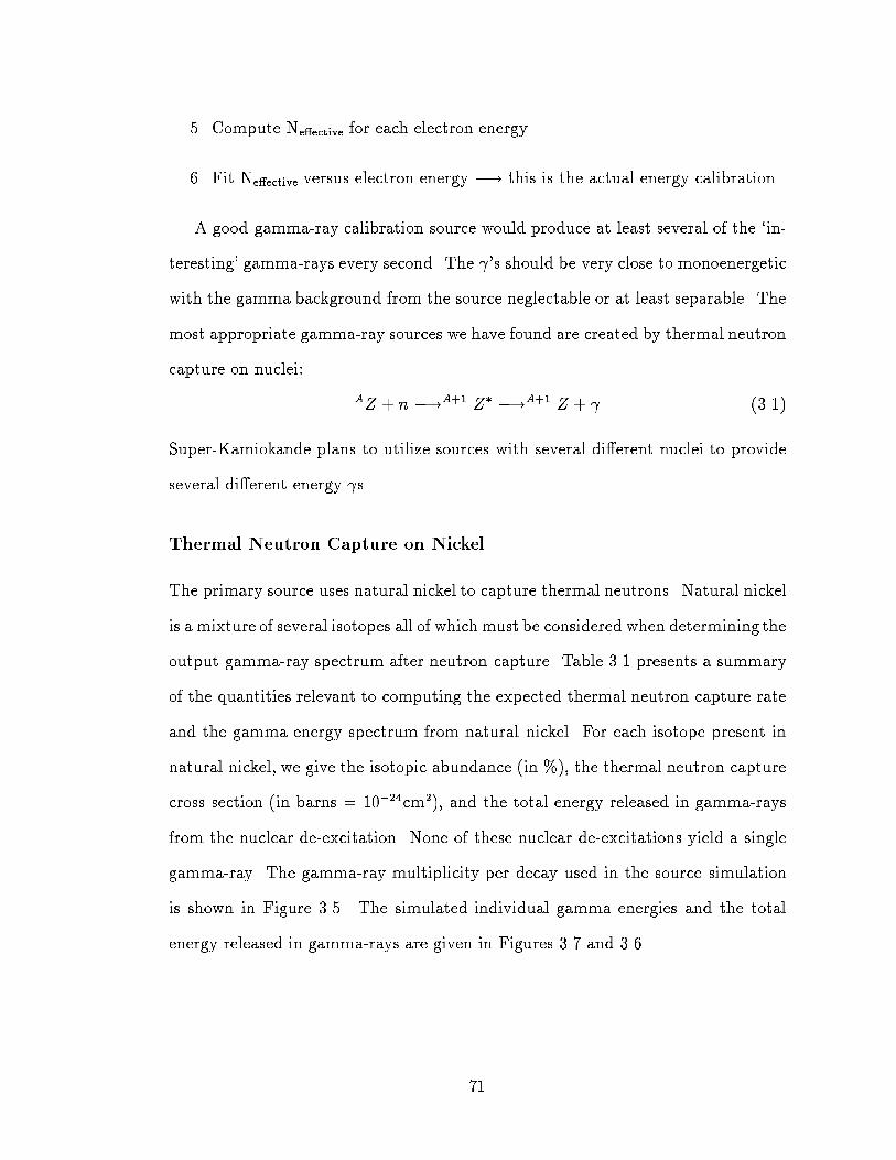
5. Compute Ne�ective for each electron energy
6. Fit Ne�ective versus electron energy �! this is the actual energy calibration
A good gamma-ray calibration source would produce at least several of the `in-
teresting' gamma-rays every second. The 's should be very close to monoenergetic
with the gamma background from the source neglectable or at least separable. The
most appropriate gamma-ray sources we have found are created by thermal neutron
capture on nuclei:
AZ + n �!A+1 Z� �!A+1 Z + (3.1)
Super-Kamiokande plans to utilize sources with several di�erent nuclei to provide
several di�erent energy s.
Thermal Neutron Capture on Nickel
The primary source uses natural nickel to capture thermal neutrons. Natural nickel
is a mixture of several isotopes all of which must be considered when determining the
output gamma-ray spectrum after neutron capture. Table 3.1 presents a summary
of the quantities relevant to computing the expected thermal neutron capture rate
and the gamma energy spectrum from natural nickel. For each isotope present in
natural nickel, we give the isotopic abundance (in %), the thermal neutron capture
cross section (in barns = 10�24cm2), and the total energy released in gamma-rays
from the nuclear de-excitation. None of these nuclear de-excitations yield a single
gamma-ray. The gamma-ray multiplicity per decay used in the source simulation
is shown in Figure 3.5. The simulated individual gamma energies and the total
energy released in gamma-rays are given in Figures 3.7 and 3.6.
71
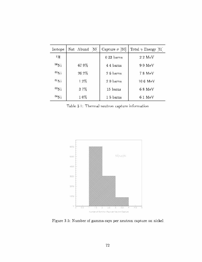
Isotope Nat. Abund. [50] Capture � [50] Total Energy [51]
1H 0.33 barns 2.2 MeV
58Ni 67.9% 4.4 barns 9.0 MeV
60Ni 26.2% 2.6 barns 7.8 MeV
61Ni 1.2% 2.0 barns 10.6 MeV
62Ni 3.7% 15 barns 6.8 MeV
64Ni 1.0% 1.5 barns 6.1 MeV
Table 3.1: Thermal neutron capture information
Figure 3.5: Number of gamma-rays per neutron capture on nickel
72

Figure 3.6: Gamma-ray energies from neutron capture on nickel
Figure 3.7: Total energy released in gamma-rays per neutron capture on nickel
73

Neutron Source
A traditional source of neutrons is the spontaneous �ssion of Californium-252 [52].
Approximately 97% of the time 252Cf decays via an � while the remaining 3% of the
decays undergo spontaneous �ssion (SF). The half-life of 252Cf is 2.65 years. There
are an average of 3.76 neutrons produced per �ssion. The average neutron energy
is 2.1 MeV and the spectrum extends up to �14 MeV. This source was chosen since
the maximumallowable source activity that could be used at the Super-Kamiokande
site was 100 �Curie and 252Cf yields the most neutrons per �Curie of activity. The
neutrons must be thermalized (moderated) before the interaction with the nickel
can proceed. The neutrons loose energy by elastically scattering o� the protons in
water. It takes approximately 19 n-p scatters (several cm of travel) and a few �s
for a 2 MeV neutron to lose enough energy to be considered thermal [53].
Source Geometry
We need to use the nickel and 252Cf together to provide an isotropic source of
gamma-rays. Since the thermal neutron capture cross section is so small, we want
to minimize the loss due to absorption in the nickel. This is easily done by
minimizing the apparent thickness of the nickel. Long strands of nickel wire are
mixed with a light material which can moderate the neutrons (like water) such
that the average density which the gammas traverse is small. The �nal source
con�guration uses a cylindrical polyethylene container 20 cm in diameter and 20 cm
tall (see Figure 3.8). Inside the polyethylene container is a 3:3.8 mixture by weight
of nickel and water. At the center of the polyethylene container is the 252Cf source.
This con�guration yields a nearly isotropic source of gamma-rays.
74

Nickel wire
immersed in water
Polyethylenecontainer
20 cm
20 cm
Californium - Nickel Calibration Source
Stainless steelwire handles
Fission Counter
Neutron source and
Figure 3.8: Con�guration of Cf-Ni gamma-ray calibration source
Simulation of Nickel Source
In order to understand the Cf-Ni source better, a simulation of the neutron capture
and gamma-ray production was done using the MCNP simulation package4 devel-
oped by Los Alamos National Laboratory [54]. The Monte Carlo for Neutrons and
Photons (MCNP) simulation package handles detailed particle tracking through
a variety of di�erent materials and the generation of energy spectra for certain
sources. The user must give details on the desired neutron source, the geometry
of the surrounding medium, and the output information needed. Figure 3.9 shows
the input card for our main source con�guration.
The material which the neutron traverses must be described to MCNP. Geo-
metrical descriptions are given for each `region'. Regions can have any shape (e.g.
cylindrical, spherical) and are not necessarily enclosed areas. The size of each re-
4Pei-Jar Liu and Bob Haight provided a tremendous amount of assistance in learning how to
use MCNP.
75

gion and the chemical makeup of the region are given with the shape. The �rst
section in the example input card de�nes the 4 `cells' or `regions' using the geomet-
rical objects listed in the second section of the input card. The source area (cell
#4) is de�ned as the volume inside cylinder #4, below plane #5, and above plane
#6. The region with the nickel in it is de�ned as being on the `outside' of surfaces
#1, 2, and 3 and 'inside' the surfaces #4, 5, and 6. This is really just the volume
between two cylinders of di�erent radii and heights. Cell #4 (#3) has a density of
1 g/cm3 (1.4 g/cm3) and is composed of material #1 (#2).
MCNP can simulate many di�erent neutron sources, including californium, by
looking up the source properties in a library. By specifying the spatial and time
distribution of each source, any geometrical source con�guration can be modeled.
Multi-source combinations can also be accommodated. In our case, MCNP was
given a `source input card' (see section 3 of Figure 3.9) which described a point
source of 252Cf at the origin. The neutron energies will be chosen from the Watt
spectrum given the parameters appropriate for californium. Finally, the chemical
makeup of each material is given. Material #1 is simply water (H2O). Material #2
is an equal mixture (by weight) of water and natural nickel.
From the MCNP simulation we extract a lifetime of 83 �s for the neutron in
the water/nickel environment. We examined the gamma-ray energy spectrum and
identi�ed the peaks due to neutron capture by protons (in the water) and by nickel.
The distributions agreed fairly well with our expectations based on knowledge of
the nuclear de-excitations. The fact that MCNP veri�ed our predictions gives us
con�dence in our understanding of the nickel source.
76

Cell Mat Dens Shape/Region What particles to use?
1 0 7:8:-9 imp:n=0 imp:p=0 !outside world
2 1 -1.00 -7 -8 9 (1 : 2 : -3) imp:n=1 imp:p=1 !water barrel
3 2 -1.40 -1 -2 3 (4 : 5 : -6) imp:n=1 imp:p=1 !nickel area
4 1 -1.00 -4 -5 6 imp:n=1 imp:p=1 !source area
1 cz 10. ! cylinder around z axis with R = 10 cm
2 pz 10. ! plane at z = 10 cm
3 pz -10. ! plane at z = -10 cm
4 cz 2. ! cylinder around z axis with R = 2 cm
5 pz 5. ! plane at z = 5 cm
6 pz -5. ! plane at z = -5 cm
7 cz 10.5 ! cylinder around z axis with R = 10.5 cm
8 pz 10.5 ! plane at z = 10.5 cm
9 pz -10.5 ! plane at z = -10.5 cm
c isotropic point source at (0,0,0) in cell 4
sdef erg=d1 pos=0 0 0 cel=4
sc1 Californium fission spectrum using Watt spectra
sp1 -3 1.025 2.926
m1 1001 .667 8016 .333 ! water
mt1 lwtr ! use the light water library
m2 1001 .667 8016 .333 28000.51c 1. ! 50% water, 50% natural nickel
Figure 3.9: Input card for MCNP
77

Fission Trigger
There are several complicated issues related to using the Cf-Ni source for energy
calibration, the �rst of which is triggering on the events. When matching the mea-
sured energy distribution to that expected for the nickel de-excitations, any energy
dependant e�ects can distort the spectrum and add a systematic error in the energy
scale. The trigger e�ciency as a function of energy can certainly cause spectral dis-
tortions. We therefore need a method of triggering on the nickel s in an energy
independent way. This can be done by simply lowering the trigger threshold until
the trigger e�ciency is at for the entire energy range of the nickel gammas. If
the trigger threshold (50% e�ciency point) is dropped to 2.5 MeV the detector
trigger rate is then almost 14 kHz. The data acquisition system can not handle
this high rate for an extended period of time. We therefore need another method
of triggering the Super-Kamiokande detector during calibrations.
The second problem is identifying which individual events come from the source
and which events are background for the calibration. Normally this can not be ac-
complished, which makes average background subtraction a necessity to isolate the
energy spectrum from the nickel source. One possible way to handle this is to
take data `on-source' and `o�-source' and do a simple subtraction. In our case,
`on-source' means Cf-Ni and `o�-source' implies Cf only. To do this, the Super-
Kamiokande tank must be opened and the nickel removed from the container sur-
rounding the Cf. Having the tank open and exposing the PMTs to ambient light
introduces problems with this method of background subtraction.
We have devised a way to solve the trigger and background subtraction problems
simultaneously. We use an ionization counter to detect the Cf �ssion products. By
78
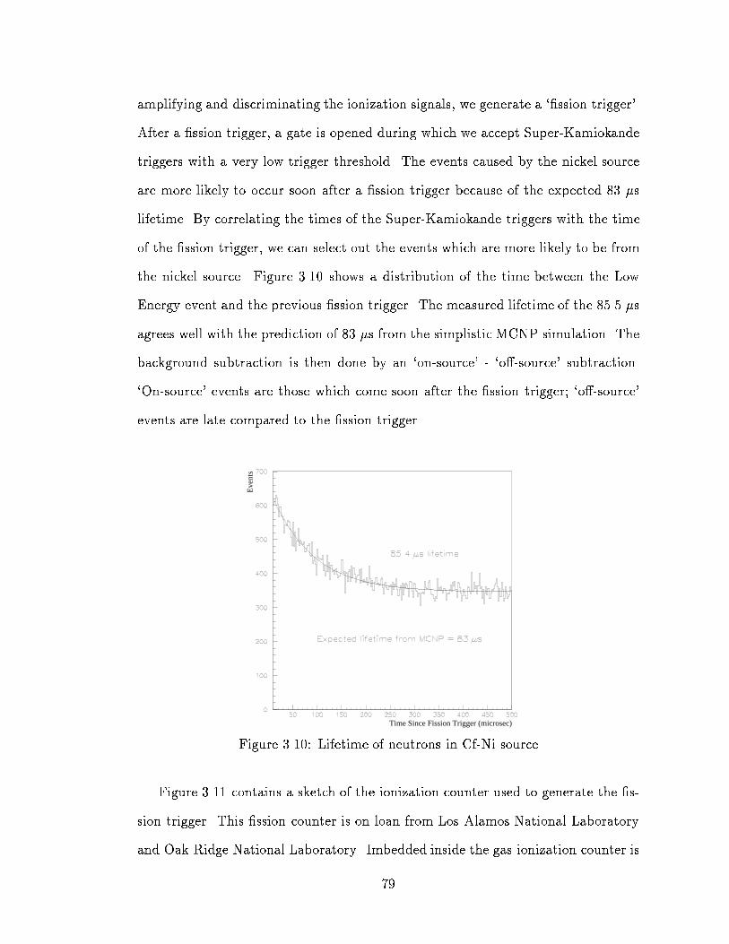
amplifying and discriminating the ionization signals, we generate a `�ssion trigger'.
After a �ssion trigger, a gate is opened during which we accept Super-Kamiokande
triggers with a very low trigger threshold. The events caused by the nickel source
are more likely to occur soon after a �ssion trigger because of the expected 83 �s
lifetime. By correlating the times of the Super-Kamiokande triggers with the time
of the �ssion trigger, we can select out the events which are more likely to be from
the nickel source. Figure 3.10 shows a distribution of the time between the Low
Energy event and the previous �ssion trigger. The measured lifetime of the 85.5 �s
agrees well with the prediction of 83 �s from the simplistic MCNP simulation. The
background subtraction is then done by an `on-source' - `o�-source' subtraction.
`On-source' events are those which come soon after the �ssion trigger; `o�-source'
events are late compared to the �ssion trigger.
Time Since Fission Trigger (microsec)
Eve
nts
Figure 3.10: Lifetime of neutrons in Cf-Ni source
Figure 3.11 contains a sketch of the ionization counter used to generate the �s-
sion trigger. This �ssion counter is on loan from Los Alamos National Laboratory
and Oak Ridge National Laboratory. Imbedded inside the gas ionization counter is
79

a 252Cf source with an activity of �1.5 �Ci. This source emits neutrons at a rate of
�1, 700 neutrons/sec. The signal from the gas ionization counter is separated from
the bias voltage (-200 Volts) and ampli�ed (factor of 40) by a pre-ampli�er (see Fig-
ure 3.12). The pre-ampli�er has two output signals: \energy" and \timing". The
\energy" output is designed to yield an accurate charge or energy measurement.
This pulse has a rise time of about 200 �s and a fall time of �100 �s. The \timing"
output is similar to the derivative of the \energy" pulse; it is intended to give a
fast timing signal so the rise time is quick (10 ns) but the fall time is still fairly
long (�100 �s). The \timing" signal is ampli�ed again, inverted, and discriminated
to produce the �ssion trigger signal. The pulses created by the alpha decay of Cf
are clearly visible above the noise. The neutron induced pulses are well separated
from the alpha induced pulses (by a factor of 5 in pulse height). The discriminator
threshold is set at 32 mV to yield a nearly perfect e�ciency for triggering on the
neutrons. The rate of �ssion triggers can be pre-scaled down by any factor so that
the total detector trigger rate is low enough to accommodate the DAQ.
For a �xed time after each (pre-scaled) �ssion trigger, Super-Kamiokande trig-
gers are accepted with a very low trigger threshold. The trigger threshold must
be low enough in energy so that there is no variation in the trigger e�ciency for
the nickel events. The chosen threshold for the Super-Low Energy threshold is
150 mV (�15 PMT hits during the 200 ns coincidence window) which nominally
corresponds to a 2.5 MeV energy threshold. Since the average time between �ssions
is �580 �s, the gate width is �xed at 500 �s. The �ssion trigger uses the Calibra-
tion I input to the TRG and the Super-Low Energy trigger uses the Calibration II
input. A typical background subtraction assumes the \nickel signal" occurs from
10 to 210 �s after the �ssion trigger while the \background" occurs from 300 to
80

2
&%'$v- �1 inch
������
XXXXXX
XXy
QQQQQQs
3% CO
Ionization Fission Counter
�
�
�
gas mixture
97% Argon
Aluminum container
SMA connector
LEMO cable
Structural Components
Sphere covered with Californium
Figure 3.11: Diagram of the ionization counter used as a `�ssion trigger'
500 microsec
-� -
6
-
-
PPPPPPq
������>
-
-200 V
Coinc
SupplyHV
AmpPre-Amp
HV
IonizationCounter
Disc
clock
1 kHz GateGenerator
window
1.7 kHz
pre-scaled\�ssion trigger"
11 Hz
Fission Trigger
\timing"output
HV + signal
Figure 3.12: Diagram of the electronics behind a `�ssion trigger'
81

500 �s (see Figure 3.10). This will provide a clean \nickel only" sample but obvi-
ously does not contain 100% of the events caused by nickel gamma-rays. Example
distributions of Ne�ective (see Section 7.4.2) from the \signal" and \background"
regions are shown in Figure 3.13 along with the background subtracted histogram.
Figure 3.13: Example of performing �tfission background subtraction
Thermal Neutron Capture on Other Materials
In addition to the nickel source, we searched for additional materials which could
be used for gamma-ray calibration. Two other metals in natural form were cho-
sen: titanium and iron. Titanium provides clean 6.8 MeV gamma-rays. Iron yields
many di�erent gammas with the most common having 7.6 MeV. Table 3.2 gives the
quantities needed to calculate the thermal neutron capture rates and the gamma
energy spectra. These nuclear de-excitations do not yield single gamma-rays. The
gamma-ray multiplicities per decay are shown in Figure 3.14 and 3.15. The indi-
vidual gamma energies and the total energy released in gamma-rays are given in
Figures 3.16 through 3.19. The �rst titanium data was taken recently and the iron
source has not yet been used.
82

Isotope Nat. Abund. [50] Capture � [50] Primary 's in Coinc.[51]
46Ti 8.0% 0.6 barns 7.3 MeV and 1.6 MeV
47Ti 7.4% 1.6 barns 7.2, 2.2, and 1.3 MeV
48Ti 73.8% 7.8 barns 6.8 and 1.4 MeV
49Ti 5.5% 1.8 barns 6.8, 1.5, 1.6, and 1.1 MeV
50Ti 5.3% 0.14 barns 5.2 and 1.2 MeV
54Fe 5.9% 2.2 barns 9.3 MeV in 1 or 2 s
56Fe 91.6% 2.6 barns 7.6 MeV in 1 or 2 s
57Fe 2.2% 2.4 barns 10.0 MeV in 2 or more s
Table 3.2: Additional thermal neutron capture information
Figure 3.14: Number of gamma-rays per neutron capture on titanium
83

Figure 3.15: Number of gamma-rays per neutron capture on iron
Figure 3.16: Gamma-ray energies from neutron capture on titanium
84

Figure 3.17: Total energy released in gamma-rays per neutron capture on titanium
Figure 3.18: Gamma-ray energies from neutron capture on iron
85

Figure 3.19: Total energy released in gamma-rays per neutron capture on iron
3.3.5 LINAC
Since the solar neutrino events are really electron events, it is natural to want to
use electrons for the energy calibration. That way, the calibration source and the
physics source di�er only in the energy spectra. It is, however, di�cult to develop
an electron source suitable for a 1% energy calibration in the 5-15 MeV energy
range. A source of electrons is needed which are monoenergetic with an energy
known to < 1%, emitted one at a time, and deposited into the Super-Kamiokande
tank. Several years ago, plans were developed to install a linear accelerator near
the Super-Kamiokande site. The LINAC would generate the desired electrons to
be deposited via a beam pipe into Super-Kamiokande.
A medical grade LINAC (Mitsubishi ML15M-III) was purchased from a hospital
and suitably modi�ed to produce the desired electrons [55]. The original electron
gun provided a current of several hundred mA. This current was much too high for
our purposes, so we built a new electron gun which draws only 50 �A. These elec-
86

trons are accelerated down a 1.7 m tube. The �nal electron energy can be adjusted
between 5-20 MeV. The electrons are emitted in \bunches" 1-2 �s long. Each bunch
contains � 106 electrons. Up to 30 bunches/sec are released. The beam size at the
end of the accelerating tube is �6 mm.
The intensity of the beam needed decreased considerably so that we get only one
electron per bunch into the Super-Kamiokande tank. The beam transport system
takes care of this reduction in intensity. The LINAC itself is placed in a hollowed
out section of rock near the edge of the tank but raised above the tank top. The
beamline must bring the electron beam down to the tank top, across the tank to
the desired penetration pipe, and then bend it 90�and shoot it into the tank water.
This is all accomplished using vertical and horizontal collimators, two 15�bending
magnets, horizontal steering magnet and coil, two Q magnets, a 90�bending mag-
net, two more steering magnets, and a vertical beam pipe with an end cap. All the
magnets have �-metal magnetic shields. The beam at the end cap is �2 cm and
has a momentum spread of < 0:3%.
The quality of the LINAC data has evolved considerably since the LINAC was
�rst turned on. Two di�erent con�gurations for the end cap have been used. Both
had an exit window for the beam made of 100 �m thick Titanium. The trigger used
for the collection of LINAC data is provided by a 1 mm thick plastic scintillator
(wrapped in 15 �m Aluminum foil). The LINAC trigger is stored in the Calibra-
tion II trigger bit (see Section 2.6). The �rst end cap (used for the data taken in
December 1996) was as large as the beam pipe (�8 cm diameter) all the way down
to the exit window. On the order of 10% of the �Cerenkov photons emitted by the
low energy electrons were shadowed by this bulky end cap (actual photon loss is
87

energy dependent). Upon discovery of this problem, a new end cap was made which
tapers down from a 8 cm top to 4.3 cm at the exit window location. The data taken
in January 1997 5 with this new end cap has much less of this shadowing problem.
Only the January data will be used in this dissertation.
The beam energy is measured to an accuracy of 0.3% using a Germanium de-
tector in the beamline. The energy of the electron as it enters the water must still
be calculated from the beam energy. The energy lost in the exit window and the
trigger counter must be calculated (or simulated) and subtracted from the beam
energy. Sometimes two electrons will be emitted in one bunch. These two elec-
tron events have the potential to disturb the energy calibration accuracy up to
a few percent. Ideally, one would `clean up' the LINAC data before using it for
energy calibration. Di�erent cleaning techniques will be discussed in Section 7.4.6.
Currently, the LINAC hardware is still being tuned and studied. The long time
stability of the beam is as yet unknown. The energy calibrations of the beam are
being veri�ed. The analysis techniques applied to the LINAC data will continue to
be scrutinized before we are completely con�dent that we have achieved the desired
absolute energy calibration using the LINAC.
3.3.6 Stopped Muon Capture
There is a myriad of other types of events which can be extracted from the data and
used for energy calibration. A convenient low energy source is nuclear de-excitation
of 16N. Occasionally, stopping muons with negative charge will get captured by the
Oxygen nucleus before the muon can decay [56]. Approximately 18% of the time
5Both the January and the December data were taken with the injection position of X =
�12:4 m, Y = �0:7 m, and Z = +12:1 m.
88

[57], the capture of the muon results the interaction 16O+ �� !16 N�+ �� leaving
16N with an excited nucleus. The remainder of the captures also go to particle
unstable states which usually end up as 14 or 15N and a neutron. Often there are
gamma-rays released as the nucleus goes to the ground state, but these gamma-rays
have not been studied as a potential calibration source.
The excited state of 16N decays to the ground state via a very low energy
gamma (<0.5 MeV). Then it � decays back to Oxygen with a half-life of 7.13 s:
16N !16 O + e� + �e (Q = 10.419 MeV). There are four di�erent �nal states for
this reaction which have branching ratios >1% [58]:
Branching Ratio 16O �nal state Decay Path
28% ground none
66% 6.13 MeV excitation directly to ground
5% 7.12 MeV excitation directly to ground
1% 8.87 MeV excitation 2
Nitrogen-16 is a good calibration source because the total rate of events can be well
determined. The cross section is known fairly accurately from the di�erence in life-
times between �� and �+ [57] and the rate of stopping muons in Super-Kamiokande
is known. Approximately 80 16N events/day occur in the Super-Kamiokande vol-
ume. These events could be used to monitor changes in the water quality (amount
of light collected in PMTs) and the trigger e�ciency.
3.4 Detector Monitoring
One of the important things to consider as any experiment starts taking data is
how the behavior of the detector will be monitored. Especially at the beginning
of data collection, many things will change. Sometimes the detector performance
89
will be a�ected. A prime example is the transparency of the tank water. As the
water is re-circulated, the impurities in the water will be removed. This may cause
changes in the light absorption and scattering lengths in the tank. So for a given
electron energy, the amount of light detected by Super-Kamiokande will be time
dependent. The changing water quality will certainly a�ect the energy threshold
of the trigger, making it time dependent also. It is therefore important to monitor
the changes in Super-Kamiokande's performance.
Several methods were developed to monitor Super-Kamiokande. Two of them
use portions of the data itself while a third uses an external source. One technique
uses the through-going muon events to extract an average attenuation length for the
water on a daily basis. Similarly, this analysis uses the spallation events to monitor
the water quality (see Section 7.3 for explanation of spallation and Section 7.4.5 for
the details of the time dependent energy scale study).
The third idea was to install a device which produces short bursts of light whose
intensity is always the same. The rate of bursts will need to be constant over time.
The device would be turned on or o� at will. On a weekly basis (or whatever the
desired time scale), this device is turned on and a calibration run is taken for �xed
time period. Both the trigger e�ciency and the number of detected PMT hits can
then be monitored as a function of time. The number of light bursts from the
source during the run can be calculated from the burst rate and duration of the
calibration run. The number of triggers recorded during the calibration run will
remain the same with time if the trigger e�ciency does not change. A drop in the
number of triggers would indicate a reduction in the trigger e�ciency. Similarly,
since the burst intensity is constant, the distribution of the number of PMT hits
90

should not change if the detector behavior is not time dependent.
To apply this monitoring concept, we need a source of quick bursts of light. The
intensity of the burst should approximately equal the same number of �Cerenkov
photons that a 5-7 MeV electron in water would produce. The time duration of
the burst should be about the same as the length of time over which �Cerenkov
photons are emitted from the electron. We decided to use plastic scintillator with a
radioactive source imbedded inside. This scheme has the potential to satisfy both
the burst duration and burst intensity requirements, depending on the scintillator
and source chosen. For a charged particle with a given energy, the number of pho-
tons emitted by most plastic scintillators will be much higher than the number of
�Cerenkov photons produced in water. By taking advantage of this increased con-
version e�ciency, we can reduce the required energy from a radioactive source of
monoenergetic electrons. We could also switch to an alpha source if the total burst
intensity meets our design criteria.
After considering the scintillator and source choices, the best option was chosen
and the sources were manufactured. The radioactive source was 244Cmwhich decays
via either a 5.81 MeV � (77%) or 5.77 MeV � (23%): 244Cm �! � +240 Pu. This
source was rated the best choice based on its half-life (17.6 years) and the negligible
background produced by the source. The half-life must be fairly long compared to
the time over which we want to use the source (several years) so that the source
activity does not change appreciably while we use it. Several other isotopes decay
with appropriate half-lives and similar � energies, but they emit gamma-rays or
X-rays along with the �. Gamma-rays and X-rays can both deposit energy in the
scintillator, creating background photons that will be seen by Super-Kamiokande.
91

The gamma-rays have a large enough radiation length (�38 cm) that their energy
deposition in the scintillator can be neglected by using a small enough piece of
scintillator. The energy deposition of the X-rays was much harder to ignore, so we
chose the source with the smallest X-ray emission.
Most plastic scintillators emit the photons within a few nanoseconds after the
particle deposits the energy. This is an acceptable time scale for the burst duration
since it is on the order of or smaller than the time resolution of the inner detector
PMTs. Also, most plastic scintillators produce photons with wavelengths in the
blue region. The chosen scintillator is Bicron 490, which comes in multi-component
form and is mixed and cast by the user. We considered embedding into the scintil-
lator a small sphere whose surface was covered with the source. A 5.8 MeV � will
travel only a few �m in the scintillator before it looses all its energy. The scintil-
lator region where the alphas deposit energy would be highly concentrated at the
sphere, encouraging saturation of the scintillator near the sphere. Saturation would
cause the scintillation e�ciency to gradually drop thereby inducing the number of
emitted photons to decrease with time. To eliminate this potential problem, the
radioactive source was uniformly dissolved in the scintillator material prior to the
plastic scintillator being formed and hardening. This con�guration prevents satu-
ration of the scintillator by spreading out where the decay alphas are depositing
energy in the scintillator. Since we needed to cast the scintillator after the source
is mixed in, our only available scintillator choice was the Bicron 490.
Bicron 490 scintillator generates light with a timing resolution of �2 ns. The
wavelength distribution is peaked at 420 nm and has a full width at half maximum
of 25 nm. The number of photons emitted by the standard Bicron 490 scintillator
92

for each 244Cm � decay (the intensity of each burst) turned out to be equivalent to
the �Cerenkov light deposition from a �30 MeV electron. This high intensity could
be useful to have, but a reduction in burst intensity of a factor of 5-6 is required to
monitor the trigger e�ciency. Discussions with several chemists at Bicron uncov-
ered a way to reduce the scintillation e�ciency to the desired level with negligible
side e�ects. A quencher was added to the scintillator to reduce the e�ciency by a
factor of 5.5 (result called Bicron 490x).
Isotope Products Inc. manufactured the sources, from the 244Cm preparation
to the casting of the scintillator + 244Cm mixture. The �nal shape of the source is
a solid cylinder 2.5 cm in diameter and 2.5 cm tall. The 244Cm activity is 1.35 nCi
which implies a burst rate of 50 Hz. Two sources with each scintillator type (490 and
490x) were made for Super-Kamiokande use. The equivalent electron energies which
produce the same photon deposition from �Cerenkov light is �6 MeV and �30 MeV.
Information from Isotope Products and Bicron regarding previous sources of this
type indicated that these `scintillator sources' would be stable sources of light for
many years. Unfortunately, the only way to turn the source on and o� is to take it
in and out of the Super-Kamiokande tank. Because there was no on/o� switch and
the collaboration pushed to minimize `down time' from physics data-taking, these
constant light sources are not used very often. They did however considerably help
us understand the detector behavior at the beginning of data taking.
93

Chapter 4
Simulations
A realistic model of the Super-Kamiokande detector allows us to answer design
and construction questions, explore calibration options, calculate e�ciencies, and
understand the general behavior of the detector. Our simulation program is bro-
ken into two main components: the kinematic generation of the physics event and
the detector simulation. Physics events range from solar neutrino interactions with
electrons to proton decay to the gamma-ray emissions of a calibration source. Mod-
elling the Super-Kamiokande detector itself involves tracking particles through the
water, generating and tracking �Cerenkov light approximating the PMTs and elec-
tronics, and simulating the trigger. Each of these topics is described in this chapter.
Our simulation uses the Monte Carlo (MC) technique to model our detector per-
formance. There is no analytic equation which characterizes Super-Kamiokande's
behavior. In the MC technique, every stage that an event goes through is modelled.
Events are simulated by using random numbers to choose which outcomes of the
various \interactions" the current event/particle will encounter. To learn about
how Super-Kamiokande \sees" certain physics events or how Super-Kamiokande
reacts to particular change in the physical detector, we simulate many of the reac-
tions and look at the average detector behavior. Because the entire data collection
94
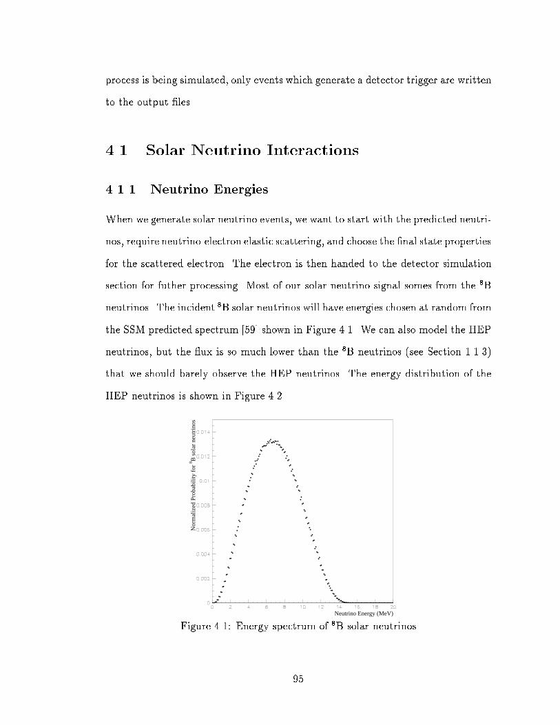
process is being simulated, only events which generate a detector trigger are written
to the output �les.
4.1 Solar Neutrino Interactions
4.1.1 Neutrino Energies
When we generate solar neutrino events, we want to start with the predicted neutri-
nos, require neutrino-electron elastic scattering, and choose the �nal state properties
for the scattered electron. The electron is then handed to the detector simulation
section for futher processing. Most of our solar neutrino signal somes from the 8B
neutrinos. The incident 8B solar neutrinos will have energies chosen at random from
the SSM predicted spectrum [59] shown in Figure 4.1. We can also model the HEP
neutrinos, but the ux is so much lower than the 8B neutrinos (see Section 1.1.3)
that we should barely observe the HEP neutrinos. The energy distribution of the
HEP neutrinos is shown in Figure 4.2.
Neutrino Energy (MeV)
Nor
mal
ized
Pro
babi
lity
for 8 B
sol
ar n
eutr
inos
Figure 4.1: Energy spectrum of 8B solar neutrinos
95

Neutrino Energy (MeV)
Nor
mal
ized
Pro
babi
lity
for
HE
P s
olar
neu
trin
os
Figure 4.2: Energy spectrum of HEP solar neutrinos
4.1.2 � � e� Scattering
Given a neutrino at a particular energy, we need to �gure out the electron energy
after the scattering has occurred. The energy dependent cross section provides this
information. We use a � � e� cross section which accounts for charged current and
neutral current interactions between the neutrino and electron. The equation for
the cross section is given by Okun [60]:
d�dTe
=2G2
FMe
�
�A+B
�1� Te
E�
��2 � gLgRMeTeE2�
for � scattering: A = g2L and B = g2R
for � scattering: A = g2R and B = g2L
gR = sin2 �W
for �e and �e: gL = +12+ sin2 �W
for �� (��) and �� (�� ): gL = �12+ sin2 �W
(4.1)
96

where :
� = scattering cross section
Te = kinetic energy of scattered electron
GF = Fermi constant
Me = mass of electron
E� = neutrino energy
�W =Weinberg mixing angle �! sin2 �W = 0:223
We use this di�erential scattering cross section to select the kinetic energy for a
scattered electron. Figure 4.3 shows the di�erential cross section versus electron
kinetic energy for two di�erent neutrino energies. We randomly pick from the shape
of the cross section when assigning a kinetic energy to a scattered electron. The
minimum kinetic energy of an electron is zero. The maximum kinetic energy for a
given neutrino energy is:
Tmax =E�
1 + Me
2E�
(4.2)
Given the energy of the scattered electron, the scattering angle is determined. The
scattering angle �scat between the neutrino direction and the electron direction is
given by:
cos �scat =1 + Me
E�
(1 + 2Me
Te)1=2
(4.3)
4.2 Particle Tracking
Once the kinematics of the physics (or calibration) event has been determined, each
particle is followed along its path until it interacts or looses all of its kinetic energy.
The EGS4 [61] package simulates the electromagnetic shower created by electrons
(e�), positrons (e+), and gamma-rays ( ). The approach taken by EGS4 is to watch
the initial particle take short steps forward along the calculated trajectory. The
97

Electron Kinetic Energy (MeV)
Diff
eren
tial S
catte
ring
Cro
ss S
ectio
n (1
0-
44 c
m2 M
eV-1
)
Figure 4.3: Energy dependence of scattering cross section for several E�
continuous loss in energy along the step length is included. Discrete processes such
as multiple Coulomb scattering (MCS) and point interactions are considered at the
end of each step. When additional particles are generated or given kinetic energy,
they are added to the `particle stack'. When EGS4 is �nished tracking a particle,
it grabs a new particle o� the stack and starts following the new particle.
EGS4 is used basically as a `black box' program. EGS4 is con�gured to know
the detector geometry (a big cylinder 41 m � 39 m�) and materials (water). To en-
sure that MCS is modelled accurately for energies <20 MeV, the energy-dependent
minimum step size that an electron may take is shortened from the EGS4 default
value [62]. The shortest step size is set so that the largest fractional energy loss
during the step is: 1.0% [63]. MCS changes the direction of travel of electrons in
the water. The average MCS angle [72] is shown in Figure 4.4 as a function of
electron energy. It is important to simulate accurately the amount of scattering
an electron undergoes in the water so that the angular accuracy of the direction
resonstruction algorithms is reproduced by the Monte Carlo.
98

Generated Total Electron Energy (MeV)
Mea
n S
catte
ring
Ang
le (
degr
ees)
Figure 4.4: Average multiple Coulomb scattering angle for H2O used by EGS4
Other types of particles are tracked through the water with GEANT [64]. We
use GEANT in a rather unusual mode. GEANT is allowed to follow a particular
particle (by taking short steps) until its �rst interaction. The products of the
interaction are returned by GEANT. If any e�, e+, or 's are produced, they are
given to EGS4. Other particles are added to a `particle stack' (separate from the
one used by EGS4). We hand particles from this stack to GEANT one at a time.
Interactions are simulated and particles are added to/removed from the stack until
the stack is empty. Once the stack is empty and all the electromagnetic particles
are processed by EGS4, the physics event is �nished being simulated.
4.3 �Cerenkov Light Generation and Tracking
Every time a charged particle takes a step through the water via EGS4 or GEANT,
our �Cerenkov light package is called. This custom-written simulation code gener-
ates the �Cerenkov light in the detector and follows the photons around the detector
99

until they `die' or are detected by a photomultiplier tube.
�Cerenkov radiation is emitted from charged particles as they travel in a medium
faster than the speed of light in the medium ( cnwhere n is the index of refraction
of the medium). The threshold velocity (� = vparticlec
) for the emission of �Cerenkov
radiation is
�threshold =1
n(4.4)
�Cerenkov photons are generated uniformly along each segment of charged particle
track. The number of photons generated per unit of tracklength in each wavelength
interval by a particle with charge ze is:
d2Nphotons
dld�=
2��z2
�2sin2 �c (4.5)
where l is the particle track length, � is the wavelength of the �Cerenkov photon, �
is the �ne structure constant (� 1137
), and �c is the �Cerenkov angle. The photons
do not all have the same energy (wavelength). The wavelengths are distributed like
1�4. The photons are emitted with directions lying on the surface of a cone with
half angle (�c) such that
cos �c =1
n(�)�(4.6)
where n(�) is the wavelength dependent index of refraction of the medium. The
�Cerenkov angle is equal to 42� for most of the life of a charged particle. As the
particle slows down, � get smaller and the �Cerenkov cone collapses down to the
central axis of the cone. The photons are polarized such that the polarization di-
rection ~p = ~vphoton � ~vparticle is normal to the travel directions of both the photon
and the charged particle.
Once �Cerenkov photons are generated, they must be tracked through the detec-
tor. There are many di�erent `interactions' which �Cerenkov photons undergo:
100

� absorbed by the water
� scattered in the water
� re ected o� the PMT face
� transmitted through the face of the PMT
� create a photoelectron in the photocathode
� absorbed by the black sheet (ID only)
� re ected o� the black sheet (ID only)
� re ect o� a waveshifter (OD only)
� absorbed by the waveshifter (OD only)
� scattered in the waveshifter (OD only)
� re-emitted by the waveshifter (OD only)
� re ected o� the Tyvek walls (OD only)
� absorbed by the Tyvek walls (OD only)
The photon simulation package accepts one photon at a time and tracks that pho-
ton until it \disappears" or is detected. Before each step begins, distances to the
next interaction of each variety listed (water absorption, water scattering, hitting
a \geometry object" like a PMT) are chosen randomly. This is done by choosing a
random probability for each `interaction' and relating it to the characteristic length
for the `interaction'. The photon trajectory is followed in discrete steps of length
equal to the shortest distance to the next interaction. After the step is taken, the
interaction is executed. If the photon has not `died' during the interaction, another
step is chosen and performed. When a photon approaches the outer edge of the
inner detector, it will either hit a PMT face or the black sheet which �lls the space
between the ID PMTs. If the photon was scheduled to hit the face of a PMT,
certain tests must be performed before the photon can be further tracked.
101
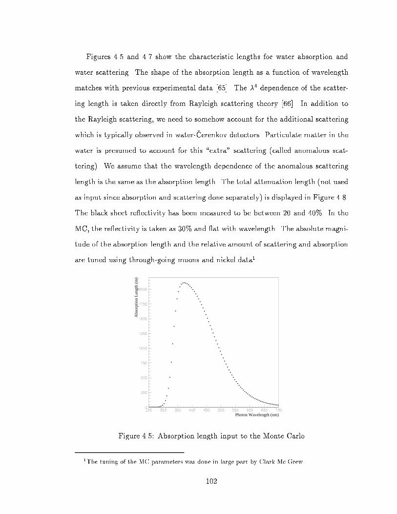
Figures 4.5 and 4.7 show the characteristic lengths for water absorption and
water scattering. The shape of the absorption length as a function of wavelength
matches with previous experimental data [65]. The �4 dependence of the scatter-
ing length is taken directly from Rayleigh scattering theory [66]. In addition to
the Rayleigh scattering, we need to somehow account for the additional scattering
which is typically observed in water-�Cerenkov detectors. Particulate matter in the
water is presumed to account for this \extra" scattering (called anomalous scat-
tering). We assume that the wavelength dependence of the anomalous scattering
length is the same as the absorption length. The total attenuation length (not used
as input since absorption and scattering done separately) is displayed in Figure 4.8.
The black sheet re ectivity has been measured to be between 20 and 40%. In the
MC, the re ectivity is taken as 30% and at with wavelength. The absolute magni-
tude of the absorption length and the relative amount of scattering and absorption
are tuned using through-going muons and nickel data1.
Photon Wavelength (nm)
Abs
orpt
ion
Leng
th (
m)
Figure 4.5: Absorption length input to the Monte Carlo
1The tuning of the MC parameters was done in large part by Clark Mc.Grew.
102

Photon Wavelength (nm)
Ray
leig
h S
catte
ring
Leng
th (
m)
Figure 4.6: Rayleigh scattering length input to the Monte Carlo
Photon Wavelength (nm)
Ano
mal
ous
Sca
tterin
g Le
ngth
(m
)
Figure 4.7: Anomalous scattering length input to the Monte Carlo
103
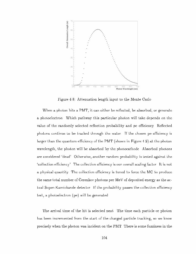
Photon Wavelength (nm)
Ove
rall
Atte
nuat
ion
Leng
th (
m)
Figure 4.8: Attenuation length input to the Monte Carlo
When a photon hits a PMT, it can either be re ected, be absorbed, or generate
a photoelectron. Which pathway this particular photon will take depends on the
value of the randomly selected re ection probability and pe e�ciency. Re ected
photons continue to be tracked through the water. If the chosen pe e�ciency is
larger than the quantum e�ciency of the PMT (shown in Figure 4.9) at the photon
wavelength, the photon will be absorbed by the photocathode. Absorbed photons
are considered `dead'. Otherwise, another random probability is tested against the
`collection e�ciency'. The collection e�ciency is our overall scaling factor. It is not
a physical quantity. The collection e�ciency is tuned to force the MC to produce
the same total number of �Cerenkov photons per MeV of deposited energy as the ac-
tual Super-Kamiokande detector. If the probability passes the collection e�ciency
test, a photoelectron (pe) will be generated.
The arrival time of the hit is selected next. The time each particle or photon
has been incremented from the start of the charged particle tracking, so we know
precisely when the photon was incident on the PMT. There is some fuzziness in the
104

Wavelength (nm)
Qua
ntum
Effi
cien
cy (
%)
Figure 4.9: Quantum e�ciency for both sets of PMTs
measured arrival photon times due to the PMT time resolution. We account for
this timing resolution by randomly picking an amount of time by which to `jitter'
the pe arrival time. We choose this `jitter time' from the measured time resolution
distribution for 1 pe signals. Figure 4.10 shows this distribution for the inner detec-
tor PMTs. The measured time of the pe is the equal to the true arrival time of the
photon plus the `jitter time'. Once the photon `dies' or generates a photoelectron,
the photon tracking package considers itself �nished and the next photon from the
current physics event is accepted.
The hits created by PMT dark noise are simulated in addition to those gen-
erated by �Cerenkov light. The number of dark noise hits allowed depends on the
average dark noise rate of the PMTs. The times of the dark noise hits are chosen
randomly in a time window much larger than the real TAC/TDC allows. The dark
noise hits all have a charge of 1 pe. Any PMT can have a dark noise hit recorded
- whether it also has a hit induced by �Cerenkov light or not. Figure 4.11 compares
the number of dark noise hits in a 200 ns time window from the MC with the same
105

Figure 4.10: Time resolution for ID PMTs
from the null triggers in the data sample. Note that the MC distribution appears
to be slightly higher than the data.
Number of dark noise induced PMT hits in 200 ns
#/bi
n
Figure 4.11: Number of ID PMT hits in 200 ns due to dark noise
Photons in the outer detector have more potential actions than those in the
inner detector. They will bounce o� the Tyvek walls quite a few times on their way
106

to the OD PMTs. The re ectivity of the Tyvek is shown in Figure 4.12. The MC
uses the measured re ectivity averaged over incident angles. The OD PMTs also
have the waveshifter plates to model. By absorbing and re-emitting the photons,
the waveshifter plates change the photon wavelengths to a more sensitive region in
the PMT e�ciency. The overall light collection is enhanced by the waveshifters,
although the timing resolution worsens by almost 50%. The simulation of the outer
detector is not critical for the solar neutrino analysis - so the detailed description
of the procedures and input parameters will not be described2.
Wavelength (nm)
Tyv
ek R
efle
ctiv
ity (
%)
Figure 4.12: Re ectivity of the Tyvek material lining the OD
4.4 Electronics Simulation
After all the photons for a single physics event have been followed, the electronics
must be modelled. The accuracy of the simulation is su�cient for our current use.
Problems apparent only when the trigger rate is very high are not included in our
model. Time dependent e�ects are not simulated (for example the real electronics
2This will probably be included in a future disseration discussing the High Energy analysis.
107

e�ects which a�ect the charge measurement of events just after energetic muons).
All the electronics parameters were matched to the values from the real Super-
Kamiokande detector (dead times, thresholds, etc.).
The electronics simulation is given a list of pes, the hit PMT numbers, and
the measured time of each hit. The photoelectrons must �rst be converted into a
charge measured by the PMT. The single pe charge distribution and the charge
discriminator threshold must be modelled. The PMT charge is selected randomly
from the shape of the single pe charge distribution (shown for ID PMTs in Fig-
ure 4.13). Note that the units of PMT charge are not real photoelectrons (see
Section 2.4). If the resultant charge is below the discriminator threshold, the `hit'
is below threshold and would not have been recorded by the real Super-Kamiokande
detector. Below threshold hits are thrown away in favor of tracking the next photon.
PMT Charge (photoelectron = picoCoulomb/2.055)
#/bi
n
Figure 4.13: Charge distribution for ID PMTs using nickel source
Above threshold hits continue through the remainder of the electronics package.
For the inner detector, the QAC gate and the dead time after each hit need to be
108

simulated. In the outer detector, the charge integration by the QTC card, edge
recording by the TDC, and digitization dead times need to be included. In both
cases, multiple pes per PMT must be accounted for properly.
If more than one pe hit the same PMT, the total charges and measured time for
the signal must be determined. The earliest pe to hit the tube sets the start time
for the PMT signal and (after the requisite time delay) opens the charge integration
gate. Other pes which later hit the same tube while the integration gate is open
will contribute their charge to the total charge for that hit. After the gate closes,
no more hits are allowed while the signal is digitized. Once the channel becomes
`live' again, the next pe (if any) in time to hit the tube will start a second signal
and open the charge gate again.
After the pes are combined together and the electronic components are simu-
lated, a list of hit tubes, times, and charges is created. This list is given to the
trigger simulator.
4.5 Trigger Simulation
The real Super-Kamiokande detector has several di�erent triggers which can cause
the detector to be read out. The Monte Carlo simulation can approximate the
Super-Low Energy, Low Energy, High Energy, and Outer Detector triggers. The
trigger algorithm is very simple for these four triggers: search through the list of hit
tubes and times looking for when the trigger condition is met. Multiple triggers can
be generated for each physics event (for example: a muon and its decay electron are
one physics event, but sometimes will produce two triggers). The trigger conditions
are given in Table 4.1. These trigger requirements were chosen to be equivalent to
109

the real detector's thresholds. The di�erence is that the MC does not attempt the
dark noise subtraction which is inherent in the ID trigger electronics. If the trigger
requirements are met at least once, the event is written out in the same format as
the real data. The PMT times are modi�ed to be a time relative to the trigger time
with most of the hits causing the trigger occurring between 800 and 1000 ns. Only
the PMT data with times in the `right' regime relative to the trigger are written
out for each trigger.
Trigger Type Condition
Super-Low Energy �24 hit ID PMTs in 200 ns
Low Energy �40 hit ID PMTs in 200 ns
High Energy �42 hit ID PMTs in 200 ns
Outer Detector �24 hit OD PMTs in 200 ns
Table 4.1: Trigger conditions for the MC simulation
The correct behavior of the trigger simulation is critical to understanding the
overall e�ciency for detecting solar neutrinos. We need a method of comparing the
e�ciency of the MC trigger to the real detector trigger. The nickel calibration data
(see Section 3.3.4) provides this key. The Super-Low Energy trigger and the �ssion
trigger are used to collect data from the nickel calibration source. In addition to
these, nickel data is typically taken with the Low Energy trigger bits set. We can
simulate this condition with the MC simply by turning on both the Super-Low
Energy and the Low Energy triggers (see Chapter 3). We can compute a relative
trigger e�ciency �trig and compare the results from data and MC. The e�ciency is
110

calculated:
�trig =# events passing the Low Energy trigger
# events passing the Super-Low Energy trigger(4.7)
as a function of reconstructed energy. Figure 4.14 show the good trigger e�ciency
agreement between data and Monte Carlo at two di�erent source locations. The
slight disagreement in the rise of the e�ciency can be attributed to the energy scale
from the Monte Carlo not perfectly matching the nickel data (see Section 8.8.2).
Reconstructed Energy (MeV)
Trig
ger
effic
ienc
y
Reconstructed Energy (MeV)
Trig
ger
effic
ienc
y
Figure 4.14: Relative trigger e�ciencies using nickel data
111

Chapter 5
Data Reduction - lef1
5.1 Introduction
Since Super-Kamiokande will see a comparatively large solar neutrino signal every
day, the size of the statistical errors on the ux measurement (among others) will
quickly become very small. Because of the small statistical errors, it is important
to get the systematic errors small and to know their magnitude with high con�-
dence. We want to maximize the potential signi�cance of any measurements that
may be made by understanding our systematics extremely well. For this reason,
all physics analyses are performed by two completely independent groups of Super-
Kamiokande collaborators. This dissertation describes the software components of
and results from the `O�-Site' Low Energy Analysis Group. A comparison with the
`On-Site' LE Group's results will be given in Chapter 9.
Super-Kamiokande collects approximately 1 million events or 30 GigaBytes of
raw data each day. The solar neutrino signal (about 40 events/day) is a small frac-
tion of this data size. We must sift through the data and select out events which
are likely to be generated by solar neutrinos. Since the total amount of raw data
is so formidable, we want to perform this event sorting in a manner that permits
112

future upgrades to the software. We also want to be able to reprocess data without
returning to the raw data. We therefore developed a multi-stage automatic �ltering
procedure.
Figure 5.1 shows a simple ow chart which explains the basic steps to our data
processing. Starting with the raw data, three separate �lters act on the data which
each reduce the size taken up by the data. Each of these �lters is automatic,
meaning that a Fortran or C program was written to enact the �ltering algorithms
and write out smaller data �les. This chapter describes the �rst stage �lter (lef1).
lef1 was developed such that we would never need to return to the raw data
to reprocess the data, only the lef1 output. lef1.5, lef2, and le ntuple are
described in Chapters 6 and 7.
5.2 Goals and Philosophy of lef1
We �lter the raw data by executing a custom-written program which reads in the
raw data �les, runs several algorithms, �gures out what information or events can
be removed, and writes out smaller data �les with the reduced information and
events. The most critical component of this program are the algorithms to run on
the data and the determination of what information or events we are willing to
throw away. We developed lef1 with certain things understood:
1. We want to save every potential solar neutrino event and throw away the rest
of the events.
2. Half of the data size (in bytes) is taken up by cosmic ray muons.
3. Muon track �ts are needed in order to cut out spallation events, a major
component to the solar neutrino background (see Section 7.3).
113

Raw data - collected at 10 Hz by Super-Kamiokande detector
?
`TQ Real' process - applies calibration constants to data
?
US copy process - �1 DLT/day (�30 GBytes/day)
?
lef1 �lter - �1 DLT/week
?
lef1.5 �lter - �1 DLT/2 weeks
?
lef2 �lter - �1 DLT/month
?
le ntuple - <2 GBytes of NTUPLEs/lef2 DLT
Figure 5.1: Overview of the Low Energy data �ltering
114

4. The majority of the Low Energy triggers have �t vertices near the PMTs. It is
presumed that many of our LE triggers are generated by gamma-rays entering
the inner detector. The source of these gamma-rays may be a combination
of the measured gamma-ray background emanating from the rock (produced
by decaying uranium and thorium imbedded in the rock) and the decay of
radioactive impurities in the PMT glass. Since these are background to the
solar neutrino signal, we can save only the LE events which do not have it
vertices close to the edge of the inner detector.
5. Cuts applied to the Low Energy events need to be well understood.
6. Correct identi�cation of data with problems is important.
7. Some data has serious problems: no information from part of the inner de-
tector, triggers caused by electronic crosstalk, detector "ringing" after a large
pulse height event, and other electronics glitches.
Based on our knowledge of the make-up of the data, we drafted a set of goals for
the Low Energy Level 1 Filter (lef1). These goals are listed in Table 5.1. Alongside
the goals are comments on the actual performance of lef1. The raw data �lls an
average of 1.1 - 1.2 DLTs per day. Approximately 8 raw DLT tapes �t onto a single
lef1 DLT, so one lef1 tape holds about 1 week's worth of data.
5.3 Event Classi�cation Scheme
The lef1 program attempts to classify each trigger by what type of event caused
the trigger. Based on the event classi�cation, lef1 decides if all the information
regarding the event is necessary. Sometimes all information is kept; other times we
keep everything except for the PMT hits. At this stage, an event is never com-
pletely removed from the data �les. We always keep the header information, the �t
115

Goals Achievements
� Reduce the data size by a factor of 10
� Run at twice the speed of data collection
� Minimize the # of cuts to the Low Energy
(LE) data
� Maximize the saving e�ciency for solar neu-
trino events in the �ducial volume
� Cut LE events using well-understood meth-
ods which can be reliably studied with the
detector simulation program
� Produce output su�cient for all future data
processing (no need to return to raw data)
� Reduction of �7
� Speed = 1.5 � data
rate
� p
� p
� p
� p
Table 5.1: lef1 goals and achievements
116

parameters for all attempted �ts, and the basic quantities computed or determined
by lef1 (see Appendix A). When an event is `tossed' or `thrown away', its class
becomes negative and everything is written to the output �le except the PMT data.
A `saved' event has everything including the PMT data saved to the output �le.
Operationally, a `tossed' event and `tossed' PMT data are almost identical. They
both end up having no PMT data saved. The di�erence is in the sign of the event
class. Events with negative classes are not processed further by any �ltering or
analysis programs.
The lef1 �lter can also be run in \tagging" mode when special studies are being
performed on the lef1 �lter. There are three di�erent ways (controlled by setting
the LE FILTER1 TAG environment variable) to run in tagging mode: tag `tossed'
events (1), tag PMT data (2), or do both (3). Tagging `tossed' events means ac-
tually saving them in full (but the events are identi�able by the negative class).
Tagging `tossed' PMT data means keeping the PMT data but making the number
of hit tubes negative.
When the O�-Site Analysis Groups �rst started writing software to �lter the
data, it was assumed that a single �lter program would be utilized for the Low
Energy and High Energy groups. The pieces necessary to form this combined �lter
had already started being assembled1. The Low Energy and High Energy groups
split apart to develop independent �lter programs, each starting with the original
`Level 1' �lter. lef1 is the product of the Low Energy group's development after
this split. Because of the history behind lef1, it uses quite a complicated algorithm
to categorize events. In the remainder of this dissertation, the lef1 classi�cations
1Clark Mc Grew spearheaded this work.
117

are given in italics. Table 5.2 shows the event classi�cations and the numerical
values for the event classes. The �rst step in the event classi�cation algorithm is
to see if the event is a null trigger (see next section). The second step is to look
at the size of the event. If the event has few inner detector tubes (NID tubes < 500)
than the event is small; events with a lot of ID hits (NID tubes > 500) are big.
5.3.1 Null Trigger Events
To assist in monitoring the ambient noise in the ID PMTs, normal data-taking runs
have the `null trigger' turned on. A `null trigger' signal is generated from a clock
approximately every 6 seconds and sent to the TRG module . The PMT data from
these null triggers should re ect just the PMT noise (no extra hits from �Cerenkov
light in the inner detector). lef1 �nds these events from the data by looking at
the trigger type for each event. If the `trigger id' = 16 (see Section 2.6), the event
is classi�ed as a null trigger, certain parameters about this event are added to the
null trigger histograms, and the event is thrown away.
5.3.2 Small Events
From the small events, we want to extract the solar neutrino events. These events
have �Cerenkov light induced PMT hits only in the inner detector and are com-
pletely uncorrelated with any detected light in the outer detector. Knowing this,
we need to select out those Low Energy events whose �Cerenkov light was completely
contained in the inner detector. Small events are further classi�ed as those that are
contained and those that may have had a particle in the outer detector. To do this,
lef1 does not rely on the OD trigger but looks at the number of OD hits. It must
be careful when doing this, since sometimes the OD tube data is actually a copy
from a previous trigger (such as an entering muon). Looking merely at the total
118

Event Classi�cation Class Value
Null Trigger 101
Small 103
Big 104
Small Contained 105
Small Non-contained 106
Noise 108
Low Energy 109
Big Contained 110
Null Trigger 111
Thru-� 112
Stop-� 113
Multi-� 114
Exiting 115
Up-� 116
Unknown 117
Geiji-� 119
LE Junk 120
Pedestal 121
Big Ringing 122
LE Ringing 124
OD Clipping 125
Corner Clipper 126
Table 5.2: Numerical values for the lef1 and lef2 classes
119

number of ID hits will then be deceiving. lef1 �rst determines if the OD data is a
copy. To do this, we look at the `tdc-to-trg' times which are stored for each of the 4
huts in the anti-header area of the data. For the 32 �s OD window, if the OD data
is not a copy, the average `tdc-to-trg' time will be < -31,500 ns. Events with copied
OD data are automatically called small contained events. After the OD window
size changed from 32 �s to 16 �s, the `trg-to-tdc' time for non-copy events should
have been compared to -15,500 ns. This was not done, so this method of �nding
copy events no longer works as expected2. For `new' OD data events, lef1 searches
the times of OD hits with a 200 ns time window looking for the largest number of
hits that occur in the window. If it �nds more than 20 OD hits in the window,
it is likely that there was `activity' in the OD and the event is categorized as a
small non-contained event. Small non-contained events are often stopping muons
which had a very short path length in the inner detector. For this reason, small
non-contained events are sent over to the big event section to be tested as a stopping
muon event. If fewer than 20 hits were found, the event is called small contained.
If no OD data exists, lef1 can not tell if the event is contained; it assumes the
event is a small contained one.
All small contained events are then examined for the possibility of having
�Cerenkov light-induced PMT hits. To do this, we need to determine if the number
of ID hits is consistent with PMT noise. lef1 searches the times of the ID hits to
�nd the maximum number of tubes hit in a 200 ns coincidence window (N200). If
N200 � 30 the ID appears to not have seen �Cerenkov light and the event is classi�ed
2The net e�ect of this is that too many events are thought to have copied OD data. These
events typically have no �Cerenkov induced PMTs in the ID and so are classi�ed as noise. If
the OD copies were correctly identi�ed, the events in question would have ended up classi�ed as
unknown.
120

as a noise event. Otherwise, the event is called a low energy event and handed over
to the Hayai fast vertex �tter (Section 5.4).
Hayai returns its best guess at the vertex coordinates of the event (X�t, Y�t, Z�t,
T�t) and an estimate of the believability of the �t, the goodness of �t (GOF). If the
GOF > 0.4, the �t is good enough to trust the vertex location. In this case, the
event is cut if the vertex lies within one meter of the inner detector edge or outside
the inner detector. This cut is known as the Dwall � 1 meter cut and is applied in
the following way:
RID = 1690 cm (outer radius of inner detector)
ZID = 1810 cm (top edge of inner detector)
R�t =qX2�t +Y2
�t
�R = RID �R�t and �Z = ZID � jZ�tjDwall = MIN(�R;�Z)
Events with Dwall � 1 meter are denoted saved low energy events; tossed low energy
events have Dwall < 1 meter. If the Hayai �t was not good enough to completely
believe the vertex but still an okay �t (0 < GOF < 0:4), the event is tagged as a
saved low energy event. Failed Hayai �ts are indicated by GOF = 0. Events with
failed �ts are identi�ed as tossed low energy events.
Tossed low energy events are like any other event which lef1 wants to throw
away - the PMT data is removed. Saved low energy events are not quite saved in
full. The data size of these low energy events can be reduced quite a bit if not
all the OD data is retained. lef1 only saves the OD hits which might get studied
later in the data �ltering process. Speci�cally, those hits are the ones with times
near the trigger time and any clusters of in time hits. The OD PMTs with times
between -5 �s and +1 �s are near the trigger time and are saved automatically.
121

If more than 6 OD hits occur in a 64 ns window, a time cluster has been found.
The time clusters are actually tagged on-line; the second bit in the `status' word
for each OD hit is a ag indicating if the hit passed the cluster criteria. The code
for the on-line tagging was written by a collaborator (Vladimir Chaloupka), hence
the tagging bit in the data is referred to as the `Vladi' bit. All OD tubes with the
`Vladi' bit set are saved with the event. All ID tubes are of course also saved.
5.3.3 Big Events
There are several pathways for big events to take from this point. If there are more
than 1,000 tubes hit in the inner detector, the event is checked to see if it could be
a single through-going track. Otherwise, the event is checked to see if it could be a
stopping muon. In either case, the next thing lef1 does is to locate the clusters of
hit OD tubes. A cluster is de�ned to have � 4 adjacent tubes hit within 50 ns of
each other. There is also a limit to the spread in PMT charges before a cluster is
broken up into multiple clusters. If there is no OD data for the event, the rest of
the \high energy event" handling of lef1 will not work. No-OD events with a lot of
ID hits are classi�ed as big contained events and saved in full for further processing.
Possible Through-going muons
Before spending cpu time attempting to do a precise track �t, lef1 does a bit more
to determine whether the event is really likely to be a single through-going track.
A quick check using the OD clusters is performed; for each pair of OD clusters:
� Compute the distance �d and time �t between the clusters
� If �d > 10 m and �t� �dc< 66 ns (determined empirically) �! this event
should continue being tested as a through-going track
122
This criterion was determined empirically from studying the single through-going
muon events in the data. Events that do not pass this test are tested as possible
stopping muon events.
Possible through-going tracks are next passed to the �rst track �tter, THR1 (see
Section 5.5.1). If the total time residual (�) found by THR1 is small (< 7:0) then the
event is classi�ed as a through-going muon (a�ectionately known as thru-�). When
� > 7:0 the event is called a multiple muon (multi-�) event, since most times this
is true. Thru-�s proceed to have better �tters run on them (THR2 and FSTMU).
Most of the time, after FSTMU �nishes with the event, the PMT hits are removed
from the output data �le. This step alone gives lef1 an output data size reduction
factor of almost 2. If the track directions from THR2 and FSTMU disagree by more
than 25�, the averaged track length is more than 10 meters, and FSTMU's goodness
of �t is > 2, the �t results are questionable enough that the PMTs for these events
are saved. Multi-� events have nothing else done to them until the next �lter
program. Consequently, the PMT data is always saved for multi-� events. Since
�6% of the muon events have more than one muon penetrating the inner detector
and since some of the real single through-going muons will accidentally be called
multi-� events, on the order of 10% of the muon events will have the PMT data
saved.
Possible Stopping muons
Due to time constraints during the development of lef1, only a moderate attempt
is made to distinguish stopping muons from the other high energy events. lef1
applies exactly the same algorithms to the potential stopping muon events as the
initial `Level 1' �lter did. The anis track �tter [67] is used to �nd the starting vertex
123

assuming a single track in the inner detector. If the `goodness' of the anis track �t
is > 20 then the �t is very poor. In order for the event to get to this point, it
must have had few ID tubes or not satis�ed the criteria for a thru-�. There is
nothing else which lef1 can do with this event, so it is classi�ed as unknown. If the
anis track goodness was < 20 lef1 continues to investigate the event. The remainder
of the algorithm is a remnant from the High Energy analysis group's `Level 1'
requirements. They wanted to separate possible exiting events (the interesting
ones) from stopping muons. If the anis track vertex is further than 3 m from the
inner detector edge, the event is classi�ed as exiting. The vertex is projected along
the �t direction until it lies on the inner detector wall. If there is no OD cluster
within 6 m of the projected vertex or if the OD cluster time is more than 50 ns
later than the inner detector `entry time', the event is classi�ed as exiting. If it
passes all these tests, the event is called a stop-�. The disclaimer at the beginning
of this section indicates that the e�ciency for correct tagging of stopping muons
is not very high. The PMT data is always saved for stop-�, exiting, and unknown
events.
Up-� Events
Since the Muon Analysis Group uses the lef1 output data set, lef1 needs to
select out possible upgoing muon events and save them in full. After the event
classi�cation algorithm is �nished, upgoing muon candidates can be selected out.
If the �t direction of the track(s) for the event indicates that the track(s) pointed
upward (cos � � �0:1 where cos � = +1 points straight up), the event is classi�ed as
an up-going muon (up-�). These events have the PMT data saved for the O�-Site
Muon Analysis Group.
124

5.3.4 Minimum Bias Events
Since lef1 was designed in a way that would prevent the need to return to the raw
data when future improvements are made to the software, some way was needed
to be able to check the performance of lef1 on the raw data. A `minimum bias'
sample is saved to enable the lef1monitoring. One event out of every 1, 000 events
processed by lef1 is selected for this minimum bias sample and has all information
saved independent of the event classi�cation. These events have a special class
assigned them which denotes the event as a minimum bias event but retains the
event type as determined by lef1 (1000 + lef1 class).
5.3.5 Record Keeping
We needed to keep track of the actions taken by lef1 and to monitor the perfor-
mance of lef1 for any portion of the data as the program was running. Each of the
components of lef1 create a log �le with a summary of the component's �ndings
for every subrun of data processed. An example of the event classi�cation log �le
(named dlt#.lef1.�ltlog) is given in Figure 5.2. There is a fair bit of information
computed and stored in a \lef1 zebra bank" saved in the output lef1 data �les;
more details are given in Appendix A.
5.4 Hayai Vertex Fitter
Since our desire is to reliably �t the vertex for every Low Energy event, we developed
a fast vertex �tter called Hayai3. Hayai uses a grid search technique to �nd the vertex
which maximizes a \goodness of �t" parameter.
3Hayai (which means fast in Japanese) was developed by Juilien Hsu and Bob Svoboda.
125
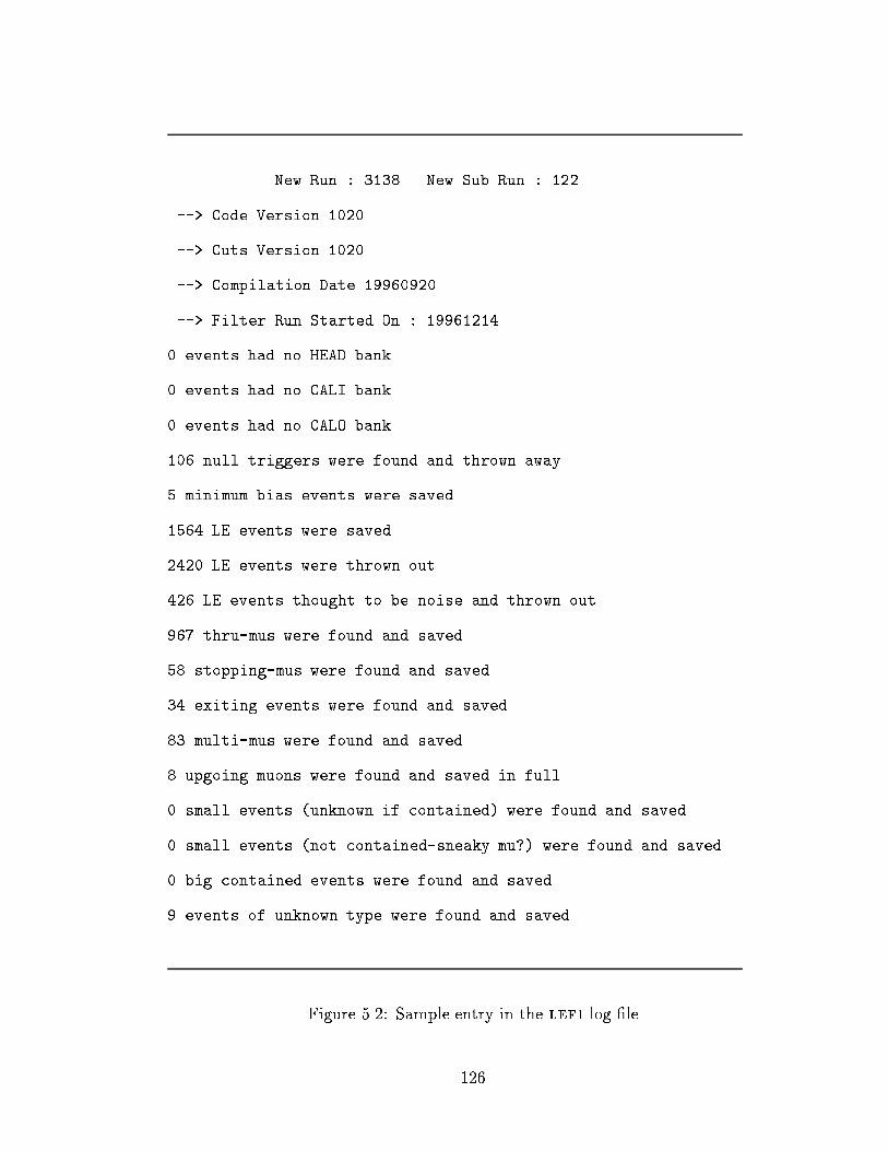
New Run : 3138 New Sub Run : 122
--> Code Version 1020
--> Cuts Version 1020
--> Compilation Date 19960920
--> Filter Run Started On : 19961214
0 events had no HEAD bank
0 events had no CALI bank
0 events had no CALO bank
106 null triggers were found and thrown away
5 minimum bias events were saved
1564 LE events were saved
2420 LE events were thrown out
426 LE events thought to be noise and thrown out
967 thru-mus were found and saved
58 stopping-mus were found and saved
34 exiting events were found and saved
83 multi-mus were found and saved
8 upgoing muons were found and saved in full
0 small events (unknown if contained) were found and saved
0 small events (not contained-sneaky mu?) were found and saved
0 big contained events were found and saved
9 events of unknown type were found and saved
Figure 5.2: Sample entry in the lef1 log �le
126

5.4.1 Algorithm
The �rst step for Hayai is the execution of an algorithm named `Mr. Clean'. `Mr. Clean'
selects which PMT hits to use for the �t, attempting to keep all the \signal" hits
while reducing the number of \noise" hits. In a typical low energy event, half or
more of the PMT hits are induced by the PMT dark current, not �Cerenkov light in
the tank. `Mr. Clean' requires that all PMT hits used in the �t must be physically
within 10 meters of another PMT which was hit within 33.3 ns. After `Mr. Clean',
the PMTs are further selected out before the maximization of the goodness of �t
begins. PMT hits from low energy events tend to be clustered together in time.
By sliding a 130 ns window through the PMT times, the largest \time cluster" of
hits is found (and contains N0 tubes). The tubes in that large time cluster are the
ones that are �nally used for the remainder of the �tting. If N0 < 5, the event can
not be �t. Hayai returns failed �ts for 0.4% (0.0%) of the 10,000 simulated 5 MeV
(10 MeV) electrons spread throughout the �ducial volume.
Hayai computes an initial vertex from which to start searching for the maximum
goodness of �t. This starting vertex is the center of mass of the PMT hits which
were selected by `Mr. Clean' and the sliding 130 ns time window. To prevent
starting with a vertex too close to the wall, all vertices are moved 2 meters away
from the wall (towards the center of the detector). The goodness of �t utilized by
Hayai ranges from 0 (bad) to 1 (good) and is given:
GOF = f(a)1
N0
N0Xi=1
exp
"�(ti � te � Toffset)2
2�2i
#(5.1)
where f(a) is a function which re ects the shape of the expected �Cerenkov cone from
the true vertex (given later in this section), a is the magnitude of the anisotropy
vector ~a, ti is the measured PMT time of the ith hit, te is the expected time of the
hit from the ith tube, Toffset is a time o�set such that (ti� te�Toffset) is centered
127

on zero, and �i is the measurement uncertainty in the time recorded by the PMT.
The anisotropy is calculated:
a = j~aj where ~a =
PN0i=1 qi
~dij~dijPN0
i=1 qi(5.2)
with ~d as the distance vector from the trial vertex (X0, Y0, Z0) to the hit PMT.
Hayai computes the expected time of the PMT hit to be:
te = T0 +
q(X0 � xi)2 + (Y0 � yi)2 + (Z0 � zi)2
vgroup(5.3)
where T0 is the time when the particle started producing �Cerenkov light, xi, yi, zi
are the coordinates of the ith PMT, and vgroup is the group velocity in water of the
photons averaged over the �Cerenkov spectrum (vgroup =c
1:395where c is the speed
of light in vacuum).
Hayai is searching for the vertex (X0, Y0, Z0, T0) which yields the maximum
value for the GOF. From the starting point, Hayai takes steps on a spherical grid
to �nd a vertex with a higher GOF. The 18 radial spokes of the spherical grid are
centered at the current `best vertex'. Including the center of the grid, there are 19
test vertices per spherical grid. The spokes of the grid lie in the following directions:
center of grid and cos � = (+1;�1)cos � = �0:75 and � = (0; �
2; �; 3�
2)
cos � = �0:25 and � = (�4; 3�4; 5�4; 7�4)
cos � = +0:25 and � = (0; �2; �; 3�
2)
cos � = +0:75 and � = (�4; 3�4; 5�4; 7�4)
The size of the grid starts out large (spokes are 8 m long) and shrinks as Hayai
closes in on the best vertex. As the grid size decreases, the uncertainty in the PMT
timing �i changes from 10.2 ns to 2.77 ns (independent of the PMT charge). The
128

anisotropy function f(a) also changes with the grid size. The spoke length follows
the sequence:
Trial number 1 2 3 4 5 6
Spoke Length (m) 8 4 2 1 0.5 0.25
For the �rst two trials, f(a) is a Gaussian of mean 0.534 and width 0.134. There
is no pattern dependence to the GOF during last four trials (f(a) = 1). For each
trial, whichever of the 19 test vertices produces a larger GOF than the `current
best vertex' becomes the `new best vertex'. As the trials are completed, Hayai
keeps track of which trial point yielded the best GOF. If N0 drops below 5 during
any of the trials, Hayai stops maximizing the GOF and returns the current vertex as
the �nal �t results. Otherwise, Hayai simply returns the best �t vertex coordinates
and the anisotropy from that vertex.
5.4.2 Performance
Hayai can �t �30 low energy events per second running on an 233 MHz Alpha
workstation. Since a cut is made based on the Hayai vertex location, we need
to understand the resultant �ts very well. We studied Hayai using two di�erent
yardsticks:
� Gaussian width of �t coordinates versus energy and location in tank
� 3-dimensional position resolution versus energy and location in tank
We �t the coordinate distributions (X, Y, Z) to Gaussian functions. The Gaussian
width (�Hayai) is the average of the widths from the �t to X, Y, and Z coordinates.
The 3-dimensional position resolution (also called the total vertex error or RHayai)
is de�ned so that 68% of the events are closer to the true vertex (or source position)
than RHayai. Where it was appropriate, we compared results on the above items
129

between calibration data and Monte Carlo simulation.
Table 5.3 contains the Gaussian widths (�Hayai) and total vertex errors (RHayai)
obtained from running Hayai on 10,000 event samples of Monte Carlo electrons gen-
erated at a single location (X = 0, Y = 0, Z given in table). The three di�erent
locations in the tank are representative of the detector center, 1 m within the edge
of the 11.7 kton4 �ducial volume, and the edge of the 22.5 kton volume.
�Hayai (1-Dim) RHayai (3-dim)
Energy Z = 0 Z = 12 m Z = 16 m Z = 0 Z = 12 m Z = 16 m
(MeV) (cm) (cm) (cm) (cm) (cm) (cm)
5 81 65 67 185 140 155
7 62 58 59 125 120 120
10 49 48 49 95 95 105
Table 5.3: 1-d and 3-d vertex resolutions of Hayai on MC electrons
Table 5.4 compares the �Hayai between the nickel data and a simulated nickel
source. Source locations with a * are outside the �ducial volume. This comparison
shows how accurately the Monte Carlo simulates the detector. Hayai �ts the Monte
Carlo nickel events and the nickel data with the same vertex resolution.
Table 5.5 compares the 3-dimensional vertex error (RHayai) for LINAC data and
MC electrons. The LINAC data was taken with the end of the beam pipe at (-
12.3 m, -0.7 m, 12.3 m). The MC electrons were simulated as a point source located
4In this thesis a ton refers to a metric ton or 1 m3.
130

Nickel Source
Source Position �Hayai Data �Hayai MC
(cm) (cm) (cm)
(35, -70, 0) 57 57
(35, -70, 1200) 56 56
(35, -70, 1600) 56 55
(35, -1200, -1200) 52 52
(35, -1200, 0) 56 56
(35, -1555, -1200) * 51 51
(35, -1555, 0) * 51 53
Table 5.4: Gaussian widths from Hayai �t on nickel data and MC
at the end of the beam pipe with directions pointed straight down. For the LINAC
data and Monte Carlo alike, the X and Y coordinate distributions are symmetric
and very well �t (small Gaussian widths). The Z coordinate on the other hand is
much wider and asymmetric. For this reason, we give only RHayai.
5.4.3 E�ect of Dwall � 1 meter cut
When we studied the �rst Low Energy data collected by Super-Kamiokande, we
discovered that the majority of the Low Energy events �t near the edge of the
inner detector. By this we mean that Hayai reconstructs the vertices of most LE
events to be within a few meters of the ID PMTs. The Dwall � 1 meter cut on the
Hayai vertex was chosen to eliminate these background events. After further study
of the reconstructed LE vertices, it was decided that the largest �ducial volume
(22.5 kton) that could be used for the solar neutrino analysis corresponded to a
131

LINAC
Beam Energy RHayai Data RHayai MC
(MeV) (cm) (cm)
5.866 195 170
6.782 155 145
8.637 140 120
15.923 85 75
Table 5.5: Total vertex errors from Hayai �t on LINAC data and MC
Dwall � 2 meter cut. We therefore need to check the e�ect of the Dwall � 1 meter
cut on events which were generated inside of the 22.5 kton �ducial volume.
We examined the e�ect of the cut on events with vertices closer than 1 meter
to the wall (events with Dwall < 1 meter are cut). Monte Carlo electrons were
simulated (including the model of the detector trigger) with locations uniformly
distributed throughout the inner detector with isotropic directions. We then looked
at the e�ciency for saving events which really had Dwall � 1 meter calculated in
the following way:
�1 =# of events which have Dwall[fit] � 1 meter
# of events generated with Dwall[MC] � 1 meter
The e�ciency �1 as a function of electron energy is shown in Figure 5.3 for ran-
domly distributed vertex locations. The values given in the graph can be explained
by the Gaussian width of the vertex resolution. Because of the resolution, events
will tend to be �t on the order of 30 cm away (in no particular direction) from the
true vertex. Due to the cylindrical shape of the detector, at any particular point
near the cylindrical edge of the inner detector there is more volume just outside the
132
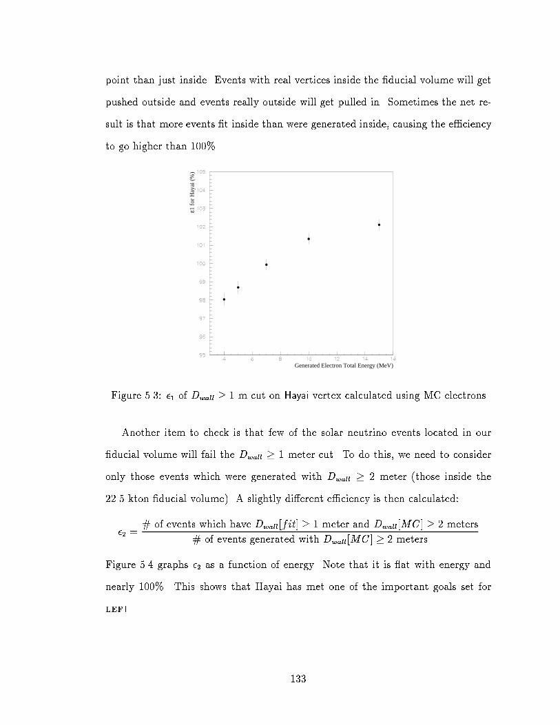
point than just inside. Events with real vertices inside the �ducial volume will get
pushed outside and events really outside will get pulled in. Sometimes the net re-
sult is that more events �t inside than were generated inside, causing the e�ciency
to go higher than 100%.
Generated Electron Total Energy (MeV)
ε1 fo
r H
ayai
(%
)
Figure 5.3: �1 of Dwall � 1 m cut on Hayai vertex calculated using MC electrons
Another item to check is that few of the solar neutrino events located in our
�ducial volume will fail the Dwall � 1 meter cut. To do this, we need to consider
only those events which were generated with Dwall � 2 meter (those inside the
22.5 kton �ducial volume). A slightly di�erent e�ciency is then calculated:
�2 =# of events which have Dwall[fit] � 1 meter and Dwall[MC] � 2 meters
# of events generated with Dwall[MC] � 2 meters
Figure 5.4 graphs �2 as a function of energy. Note that it is at with energy and
nearly 100%. This shows that Hayai has met one of the important goals set for
lef1.
133

Generated Electron Total Energy (MeV)
ε2 fo
r H
ayai
(%
)
Figure 5.4: �2 of Dwall � 1 m cut on Hayai vertex on events in �ducial volume
5.5 Track Fitting
A simple way to reduce the data size by a factor of two is to throw away the PMT
data on all the cosmic-ray muon events. We need to know the trajectories of the
muons to e�ectively remove spallation events. We perform track �ts and save the
�t information so the PMT data may be dropped. In order to be con�dent enough
about the track �t to drop the PMT hits from the event, we want to have a way to
check our �t results. Several track �tters are used by lef1 to enable this double-
checking. They are described in the following subsections in increasing order of
their �t accuracy (and decreasing order of their running speed).
The performance of single track �tters is examined on actual muon events in
the data. The only `correct' or `true' tracks we can compare with are those �t by
hand (by eye). Since the human eye excels at observing patterns, we can `�nd'
the entry point and exit point for a through-going muon event fairly easily using
a color-enhanced event display program. By comparing the hand �t tracks from
134

several people, we can estimate the angular accuracy of the hand �ts to be �1�.
5.5.1 THR1
The �rst, most simplistic, track �tter uses only the outer detector information.
The basic premise is to look for clusters of tubes in the OD which are separated in
distance and time in a manner consistent with a particle travelling from one cluster
to the other at the speed of light. The algorithm can be described as:
1. Find clusters in the hit OD PMTs
2. For each OD cluster: compute the charge weighted average position and time
of the hit PMTs �! this is the `cluster' position and time
3. Clean the ID tube hits by requiring that good hits have an immediate neighbor
hit within 4 ns
4. Sparsify the ID data by randomly choosing 10% of the tubes such that the
charge distribution of the hits is preserved (leaving Nreduced tubes to use)
5. For each pair of clusters: use the cleaned, sparsi�ed ID data and compute the
total time residual (�) for the event assuming the clusters are entry and exit
points for a single track:
� =
PNreducedi=1 (qi�i)PNreduced
i=1 (qi)� 1: : :where : : : �i = ti � Tentry 1 � dphoton
vgroup� dparticle
c
where qi is the tube charge, ti is the time of the hit, Tentry 1 is the time of
the entry cluster, dphoton is the distance the photon went through the water
from the emission point along the track to the hit PMT, vgroup is the group
velocity for �Cerenkov light in the water (vgroup =c
1:385), dparticle is the distance
along the track (from the entry point) the particle travelled before emitting
the photon, and c is the speed of light.
135

6. Keep track of which cluster pair yields the smallest �
The THR1 entry and exit points are taken as cluster positions for the pair of clusters
which gave the smallest value for �. The accuracies of the THR1 entry point and
the direction �t are given in Figure 5.5. These distributions compare the THR1
and hand �t tracks parameters on a sample of hand-identi�ed single through-going
muons from the data.
Figure 5.5: THR1 angular accuracy and entry point error distributions
5.5.2 THR2
Once an event has been tagged as a single through-going muon event, the exit point
is re�ned by the THR2 algorithm5. THR2 uses the `hot' inner detector tubes (those
with a lot of charge) to compute a more accurate exit point. The 10 PMT hits with
the largest charge are selected. The �rst iteration computes the charge weighted
position/time of the 10 hottest PMT hits and calls that the exit point. The second
iteration makes a further cut on the hot tubes to require that each tube be within
5THR2 written by Greg Sullivan.
136

20 ns and 7 m of the �rst iteration exit point. The charge weighted position is
computed again with this smaller set of tubes. For most events, the result of the
second iteration is returned as the new (better) exit point. Occasionally this second
step will throw out too many tubes (i.e. when you have a cluster of hot tubes and
one really hot tube very far away - the charge weighting pulls the average away
from the cluster towards the single tube). In this case, both iterations of THR2 are
not to be trusted and the initial OD exit point is returned. The improved angular
accuracy of THR2 is given in Figure 5.6.
Figure 5.6: THR2 angular accuracy distribution
5.5.3 FSTMU
FSTMU6 reliably �nds the track for many of the single through-going muon events
using the inner detector almost exclusively. FSTMU was designed to run fast enough
to be incorporated into the lef1 program and yet provide accurate enough �ts to the
track parameters to make spallation cuts (see Chapter 7). It is based on FASTMU,
6Tomasz Barszczak wrote FSTMU.
137
a fast track �tter from the IMB experiment.
As is typical with �tters designed for Super-Kamiokande, FSTMU �rst \cleans"
the inner detector PMT data. The objective is to remove the PMT hits which were
caused by dark noise, leaving only the hits induced by the muon's �Cerenkov light.
Cleaning requires acceptable ID hits to have at least one adjacent PMT which was
hit within 4 ns. Using the cleaned PMTs, FSTMU locates its preferred entry and
exit points, assuming that the detected light was produced by a single particle
traveling at the speed of light which enters and exits the inner detector. The basic
idea for the entry point algorithm is to �nd a bunch of tubes which are next to
each other and all have early times (compared to most of the PMTs in the event).
These early tubes will de�ne the entry point. A bit more care must be taken when
determining the exit point. The exit point will be de�ned by a set of neighboring
tubes which have the highest measured charges in the event. It is easy for the
exit point to be pulled towards the entry point. This potential bias is removed by
neglecting tubes which are closer to the entry point than two PMTs away from the
furthest `hot' PMT (steps 3b and 3c).
The entry point is chosen using the following algorithm:
1. Select the 20 earliest PMTs from the `clean ID PMTs'
2. Locate clusters within the 20 hits
3. Choose largest cluster
4. Calculate unweighted average time of the PMTs in the cluster
5. Select the PMTs which were hit earlier than the average time
138

6. Calculate the unweighted average position and time for those early hits
�! This yields the entry point and entry time
The exit point is chosen using the procedure:
1. Select 70 hottest (highest charge) PMTs from the `clean PMTs'
2. Find clusters within the hot tubes
3. For each cluster:
(a) Select PMTs which are hotter than the average charge of cluster
(b) Find PMT which is farthest from the entry point, calculate the distance
between this PMT and the entry point, and subtract twice the PMT
separation distance
(c) Reject PMTs closer to the entry point than the distance just calculated
(d) Calculate the charge weighted average position and time of the remaining
PMTs �! This yields an exit point (time) candidate
4. Compute the speed at which a particle would need to travel to go from the
entry point to each candidate exit point
5. Calculate the deviation of each `particle speed' from the speed of light
6. If the smallest deviation from the speed of light is > 0:2 � c then:
Choose the exit point (time) whose speed is closest to c
Otherwise Select the exit point (time) which is farthest from the entry point
The quality of the FSTMU �ts can be checked in two di�erent ways. The �rst is
the deviation from the speed of light of the particle speed necessary to go from the
entry point to the exit point in the time computed (exit time - entry time). The
second way is to look at the time residuals. The time residuals are the di�erence
139

between the measured time of each PMT hit and the expected time of the hit given
the particle track location, entry time, and the location of the PMT (assuming that
the light was emitted at a �Cerenkov angle of 42 �).
FSTMU �ts muons at a rate of 45 Hz as measured on a 333 MHz Alpha (by far
the slowest of the three �tters used in lef1). FSTMU's track �t accuracy on hand-
�t single through-going muons can be seen in several di�erent ways in Figure 5.7.
The �rst plot shows the distance di�erence between the FSTMU entry point and
that from the hand-�t. A distribution of the angular deviation between the track
direction found by hand and FSTMU is given in the second graph.
Figure 5.7: FSTMU angular accuracy and entry point error distributions
5.6 Trashman
One of the problems with the low energy data is that about 5% of the triggers are
unwanted \junk". Electronics noise and PMT afterpulsing often generate triggers
in which we are not interested. Sometimes an otherwise `good' event will have
140

extra PMT hits which are `junk'. Due to the manner in which the O�-Site analysis
groups acquire a copy of the data, we sometimes have several (unwanted) copies of
events or runs. Trashman7 has been designed to search out these junk-�lled events.
Several categories of \trashy events" exist including:
� Pedestal
� Crosstalk
� Ringing
� `Hut 4 noise'
� Muon-related junk
� Event number gaps
� Repeated events
� Repeated subrun
A pedestal event is an event which occurred during the pedestal taking period.
Every 1/2 hour or so some of the workstations collecting data from the inner detec-
tor switch operating modes from `normal' to 'pedestal' for a few seconds. During
this time the workstation is monitoring the pedestal values of the QACs and TACs
for each ATM the workstation controls. Normal data is taken and assembled into
events using the remaining workstations which are operating in `normal' mode. Ef-
fectively, some portion of the inner detector has no data recorded for �1 minute
period every half an hour. These events would be very tricky to deal with correctly;
vertex and track �tters would perform poorly and the energy of the events can not
be well determined. Trashman identi�es these pedestal events so they can be thrown
away (and the livetime adjusted) at a later stage using the following criteria:
1. NID tubes > 1500
7Trashman was developed by Mark Vagins.
141

2. a gap of > 500 sequential wall tubes
Sometimes a workstation drops out of the data ow for di�erent reasons (usually
indicating some problem). These `workstation drop-out' events also will get tagged
as `pedestal' events.
Electronic crosstalk between the outer and inner PMT cables (near the PMT
bases) causes hits in inner PMTs within close proximity of a particularly energetic
OD hit. The characteristic pattern of cross-talk is that rectangular patches of ID
tubes near each other are hit. Events with a lot of crosstalk hits have certain
characteristics:
1. NID tubes > 15 which each have q < 0:1 pe
2. NID tubes <NOD tubes
3
3. QID total
NID tubes
< 1:5 pe/tube
used by Trashman to tag such events.
After energetic events in the inner detector, we often get triggers generated by
electronic `ringing'. PMT afterpulsing and signal re ections on cables often cause
these triggers. `Ringing' events can be tagged by Trashman using the requirements:
1. NID tubes > 10 which each have q < 0:1 pe
2. NID tubes in Hut 4 < 20 which each have q < 0:25 pe
3. QID total
NID tubes
< 0:25 pe/tube
`Hut 4' events are caused by a persistent, localized electronics problem. It is
possible (but not convincingly proven) that insu�cient grounding of some electron-
142

ics racks in Hut 4 is the root cause of this electronics problem. Hut 4 events can
be found by:
1. NID tubes in Hut 4 > 20
2. NID tubes in Hut 4 > 10 which each have q < 0:25 pe
3. QID in Hut 4
NID tubes in Hut 4
< 0:45 pe/tube
There is a Trashman classi�cation called `muon-related junk'. Muons sometimes
travel in the dead region between the ID and OD tubes (and are called geiji or
caterpillar muons). The �Cerenkov light is incident on the backs of the PMTs causing
PMT hits, but the PMT signals are not always useful for �tting algorithms. These
caterpillar events almost always have lots of PMTs which have very low charge.
The following criteria were developed to tag these `mu-related junk' events:
1. NID tubes < 1500
2. NID tubes > 15 which each have q < 0:1 pe
3. QID total
NID tubes
> 1:5 pe/tube
The remaining event categories which Trashman searches for are gaps in the
event number within a run and repeated data. For any given run, the event num-
bers should start at one and constantly increase by one. A gap in the event numbers
would indicate a problem of some sort. Data can occur repeatedly on our data tapes
in two di�erent ways, both caused by the calibration process, `TQ real'. Sometimes
`TQ real' encounters a problem, sort of gets stuck, and stores the same event to the
ram disk over and over. Since we copy the data stored on this ram disk without
passing judgement, we copy these repeated events directly to DLT tape. Other
`TQ real' problems will cause the calibration process to require re-starting. The
process must be started at the beginning of a run (which has been changed). This
143

means that in the middle of a particular run and subrun (e.g. run 1234, subrun
56), the data being stored to the ram disk will suddenly start over at the beginning
of the run (e.g. run 1234, subrun 1). The subruns 1 through 56 will appear twice
on our data tapes. Trashman watches for these sorts of repeated data by looking
for drops in event number or subrun number within the same run and for multiple
consecutive occurrences of the same event number.
Trashman only tags the junk events it �nds using the above described algorithms.
The tag is used further in the next stage of data processing before the uninteresting
events are removed from the data sample. Trashman tags very conservatively so as
to not accidentally toss too many real solar neutrino events; if Trashman calls an
event bad, it is de�nitely bad. Consequently even once Trashman-tagged events are
tossed, there is still junk which remains in the data stream. Trashman summarizes
its �ndings for each subrun in a log �le named dlt#.lef1.trash (example given in
Figure 5.8).
5.7 SaveRun
The SaveRun routine8 collects information from each subrun which will help a later
determination of the quality of that subrun. SaveRun outputs to a log �le (naming
convention: dlt#.lef1.saverun) which is used during later data processing. SaveRun
counts the number of events per subrun without outer detector (OD) data and the
number of events without inner detector (ID) data or OD data. Blocks of no-OD
events are also recorded in the log �le. A sample subrun entry in the SaveRun log�le
is given in Figure 5.9.
8SaveRun provided by Andy Stachyra.
144

Results of trashman.c
Trashman Revision: 1.10
---------------------
New Run : 3138 Sub Run : 122
Number of events checked = 5680
O.K. events = 5489
Events with tripped OD high voltage = 0
Events with pedestals in workstation 1 = 0
Events with pedestals in workstation 2 = 0
Events with pedestals in workstation 3 = 0
Events with pedestals in workstation 4 = 1
Events with pedestals in workstation 5 = 0
Events with pedestals in workstation 6 = 0
Events with pedestals in workstation 7 = 33
Events with pedestals in workstation 8 = 52
Events with crosstalk between OD and ID = 64
Events with ringing = 24
Events with hut 4 noise = 1
Events with gap in event number = 0
Events with other muon-related junk = 25
Repeated events = 0
Repeated events due to repeated subruns = 0
Figure 5.8: Sample Entry in a Trashman Log File
145

Start of saverun job (Revision: 1.4)
RUN 3138
SUBRUN 122
First Event Number: 754904 Time: 96/11/23 18:06:50
A series of events without OD data starts at:
Run: 3138 Subrun: 122 Event: 756806
Time: 96/11/23 18:10:00
And ends at:
Run: 3138 Subrun: 122 Event: 756819
Time: 96/11/23 18:10:00
It is 14 events long.
Last Event Number: 760583 Time: 96/11/23 18:16:15
This subrun has 290 ID events missing OD data.
Figure 5.9: Sample Entry in a SaveRun Log File
146

5.8 Livetime
The Livetime routine9 computes the length of time over which every subrun extends.
In addition, a lookout is kept for blocks of pedestal events, during which we do not
consider the detector `alive'. The time durations of each pedestal-taking period is
recorded so that the dead time associated with the pedestal events can later be
removed from the total live time of the subrun. All output is saved in a log �le
named dlt#.lef1.live.
Three di�erent clocks are used to compute the live time:
1. computer
2. 48 bit
3. GPS
The reading of each clock at the trigger time is stored in the data �le for every event.
The computer clock is actually the internal clock of the online host computer. The
time stored in the data �le is in Japan Standard Time and is accurate to a second.
The 48 bit clock is the clock inside the TRG module which runs at 50 MHz. The
clock value at the trigger time is readout with the rest of the TRG information.
This is the best clock for measuring the time between events. Rollovers in the
clock value must be accounted for. The Global Positioning System (GPS) clock
is our key to the absolute time of the trigger. It is the GPS clock which will be
used to look for coincident time-varying signals between Super-Kamiokande and
other experiments. The GPS clock is latched every 21 seconds, but stored in the
data for every event. An accurate GPS time at which every trigger occurred is
desired. A VME scalar running at 50 MHz (the `local clock') is zeroed each time the
9Livetime provided by Juilien Hsu.
147

GPS clock is latched and therefore allows interpolation between the GPS latches.
Due to instabilities in the optical �ber connection between the GPS antenna and
the VME module which decodes the antenna signals, there are spurts of events
without a reasonable GPS clock time. The quality of each of the clocks is monitored
separately. Sometimes there are problems with the livetime calculation which are of
unknown origin10. Livetime also watches out for pedestal-taking periods by looking
at the event ag in the header of the data and at the output of Trashman's search
for missing workstations from the data. Information about all blocks of pedestal
events are recorded in the Livetime log �le (see Figure 5.10).
5.9 E�ciencies
5.9.1 Muon Identi�cation
We need to know the identi�cation e�ciencies of the lef1 �lter for various types of
muon events. We are most concerned with the mis-identi�cation of muons which
result in PMT hits being thrown away, removing the possibility to re-�t the event
later. The measurement of these id e�ciencies requires a sample of muon data with
known event classi�cations. A collaborator11 hand scanned and identi�ed by eye
10,207 events in order to collect a sample of 2,025 muon events. Using this sample,
the identi�cation e�ciencies were calculated by simply running the lef1 software
on the data sample and counting the number of events falling into each category.
The number of events with each lef1 classi�cation are given in Table 5.6. All the
muon events from the hand scan are present in the table. Separate event counts
are given depending on whether the PMTs would have been kept or thrown away.
10We think that rollovers in the clock values may not be properly handled.
11Thanks go out to Shige Matsuno for this performing this task.
148

Livetime Revision: 1.13
-------------------------
***START
run number: 3138 ,subrun number: 122
1st event: 754904
GPS(s,us): 848707595 41691760 Scaler: 3227895562
Computer(yr_mth_day,hr_min_sec): 961123,180650
ped_start! evt #: 755011
180657(cmpt) 848707616(gps_sec) 29277987(gps_usec)
ped_end! evt #: 755061
180707(cmpt) 848707616(gps_sec) 36882729(gps_usec)
### Ped live time: 7.604740(gps), 50(cmpt) ###
ped_start! evt #: 756055
180848(cmpt) 848707702(gps_sec) 46467100(gps_usec)
ped_end! evt #: 756127
180856(cmpt) 848707724(gps_sec) 35105958(gps_usec)
### Ped live time: 10.638860(gps), 8(cmpt) ### ... (text removed)
FINISH
last event: 760584
GPS(s,us): 848708153 37014062 Scaler, Rollovers: 1220323765 11
Computer(yr_mth_day,hr_min_sec): 961123,181615
--------------------------------------
Live time: 553.322327(gps), 565(computer), 904.737549(scaler)
Scaler live time is not usable!
Figure 5.10: Sample Entry in a Livetime Log File
149

There are many di�erent numbers given in Table 5.6. The most important
ones are those for events which have the PMT data thrown away (marked with
y). Once the PMT data is tossed, more �ts can not be performed on the event
and the classi�cation of the type of muon will not change. Of the 1,747 events
tagged as thru-�s, 95.54% of them were really through-going muons which had
their PMT data tossed. This is a fairly high e�ciency for correctly tagging single
through-going muon events. Forty seven of the thru-� events were really multiple
muons which were misidenti�ed and had their PMT data thrown out. Six stopping
muons were called thru-�s incorrectly and had their PMT data removed. These
misidenti�cations (especially the multiple muons) will result in a slightly larger
solar neutrino background rate of spallation products which pass the spallation
cuts (see Chapter 7).
Hand Fits Results
Thru-� Stopping � Multiple � Other
lef1 class # ev. 1846 62 117
Toss Keep Toss Keep Toss Keep All
Thru-� 1747 1669 y 16 6 y 1 47 y 8 0
Stop-� 129 0 74 0 17 0 0 38
Exiting 132 0 47 0 23 0 0 62
Multi-� 93 0 20 0 7 0 62 4
Up-� 8 0 8 0 0 0 0 0
Unknown 514 0 12 0 8 0 0 494
Table 5.6: Number of events in each lef1 and hand �t class for real muons
150

5.9.2 Low Energy Events
One of the crucial pieces of knowledge we need about lef1 is its e�ciency for saving
solar neutrino events generated inside the �ducial volume. To study this e�ciency,
we did several di�erent things. First, we examined the behavior of the Hayai ver-
tex �tter and the e�ect of the cut: Dwall > 1 meter. This work was described in
Section 5.4.2. Second, the e�ciency of the full lef1 �lter program was computed
on Monte Carlo solar neutrino events so that the full event identi�cation method
could be studied.
We know that due to the vertex resolution, some events with vertices actually
located outside the �ducial volume will �t inside and vice versa. Therefore, in
order to calculate the e�ciency correctly using Monte Carlo (MC) event samples,
the MC events should have vertices extending all the way up to the edge of the
inner detector (de�ned as where the `black sheet' lies). The e�ciency of the lef1
�lter for the 22.5 kton �ducial volume (Dwall � 2 meter) is then:
�3 =# of events passing lef1 with Dwall[fit] � 2 meters
# of events generated with Dwall[MC] � 2 meters(5.4)
Figure 5.11 shows �3 as a function of electron energy. The high e�ciency which is
fairly at with energy is precisely what lef1 was designed to achieve.
151

Generated Total Energy (MeV)
LEF
1 ef
ficie
ncy
for
F.V
. eve
nts
Figure 5.11: �3 of lef1 �lter on simulated electrons in 22.5 kton �ducial volume
152

Chapter 6
Data Reduction - lef2
6.1 Introduction
The output of the lef1 �lter still contains a lot of events which are not solar
neutrino candidates. The Low Energy Level 2 (lef2) �lter was designed to do
everything necessary to meet the following goals:
� Output data set is small enough to distribute to any and all collaborators
� At least keep pace with lef1 �lter
� Output contains PMT data only for solar neutrino candidate events
� Nature of output data is unquestionably good
The reduction factor from lef1 output to lef2 output is about a factor of 4.
Whereas 1 week of data �ts on 1 lef1 DLT, 1 month of data will �t onto 1 lef2
tape. lef2 more than keeps up with the lef1 processing; lef2 (running on a
333 MHz Alpha) can process �7 days of data (one lef1 tape) in 12 day. In order
to accomplish the third and fourth goals, lef2 must complete the following tasks:
� Find multiple muon events and �t the tracks
� Find stopping muons and �t track
153

� Decide what should be done with thru-� events whose lef1 �ts were ques-
tionable
� Handle the big contained events (no OD data events)
� Identify, categorize, and �t (if necessary) the unknown events
� Find a more precise vertex for the Low Energy events
� Make the `�nal' cut on vertices of Low Energy events (for largest �ducial
volume desired for analysis)
� Remove `junk' and other undesirable events
� Remove subruns or runs with problems
� Create and update a database containing a summary of the processed subruns
6.2 Good Run/Subrun Selection
The very �rst thing which lef2 wants to know is \This data which I have, is it
any good?". Information which is used to answer this question is collected by
good&bad data. Several algorithms look for various clues which may point towards
\bad" data. Each algorithm sets its own series of ags for every subrun which
are then used to tag the \bad" data. Good&bad data takes the ags from these
algorithms and combines them into a single ag which is set bit by bit (a particular
bit is set by good&bad data if a particular ag was set by one of the algorithms).
This good&bad data ag is given to lef2 which looks at the bits and decides by
itself if the data is really \good" or \bad". The determination of whether a subrun
is \good" or \bad" depends critically on the inherent philosophy behind lef2. The
154

data coming out of lef2 is to be unquestionably good. Any data which is close to
the border between \good" and \bad" is conservatively called \bad".
6.2.1 lef1 Log Files
The main source of information used to tag \bad" data is the log �les created by
the lef1 �lter program. In order for good&bad data to access this information,
the log �les must be read in and parsed for the desired information. There is a
complicated way in which good&bad data �gures out which log �les to open (there
is one `set' for each raw dlt tape processed by lef1 ) from the number of the tape
being used as lef2 input. Once the log �les are parsed, good&bad data can start
using the information to set ags.
Table 6.1 shows all of the ags set from the lef1 log �les and the criteria which
must be met to have the ag set. A `toga' log �le is one created by the main
program which is linked with the lef1 code. It has a single line for every subrun
processed which contains the run #, subrun #, �rst and last event # in the subrun,
and some other information. This information is gleaned from the data �le as the
data is processed by lef1.
Figures 6.1-6.6 show the distributions of the quantities upon which cuts are
placed. The cut values are in some cases closer to the main part of the distribution
than some would generally feel comfortable with. The cuts however re ect the de-
sired conservativeness of the data sample. The number of ID events histogram has
most of the subruns in the �rst bin, so an expanded view around the x axis is shown.
The requirement on the fraction of events in a subrun which can have no OD
155

data depends on the width of the the time window. The cut was raised from 2.5%
with the 32 �s window to 10% for the 16 �s window. The fraction of events without
OD data went up when the window was reduced. Many triggers occur right after
an energetic muon event. When the window size decreased, the hits associated with
the muon event were being digitized when the following triggers were generated.
The OD TDCs were unavailable for these triggers due to the digitization, so the
number of events without OD data increased.
The cut on the number of saved low energy events is not as stringent as it could
be, however many of the subruns above the cut and below the peak are eliminated
by the other requirements. The requirement that a run have �3 subruns comes
from experience controlling the runs. Sometimes an immediate problem will crop
up just after the run starts. Because of the time it takes to observe a problem with
the collected data and to stop the run after �nding a problem, these \immediately
aborted" runs are often one or two subruns in length (10 to 20 minutes).
Figure 6.1: Number of events in each subrun without ID data
156

Flag Criterion
Flags set on subrun basis
Repeated subrun Listed more than once in the `toga' log �le
Repeated events Total number of events processed in subrun is
> last event #� �rst event # + 1
Too many no-ID events Number of events without ID data > 10
Too many no-OD events # no-OD events# events >
8>><>>:
2.5% if 32 �s OD window
10.0% if 16 �s OD window
Too few thru-� events # thru-� events# null triggers < 8
Not enough saved low
energy events
Fewer than 100 saved low energy events
Too many noise events # noise events# tossed low energy events > 0:25
Too many saved low en-
ergy events
# saved low energy events# tossed low energy events > 1:0
Flags set on run basis
Too few subruns in run < 3 subruns recorded in `toga' log �le for the run
Table 6.1: Criteria to have Good&bad data ags set from the lef1 log �les
157

Figure 6.2: Fraction of events in each subrun without OD data
Figure 6.3: Rate of thru-� events in each subrun
158

Figure 6.4: Number of saved low energy events in each subrun
Figure 6.5: Fraction of noise events in each subrun
159

Figure 6.6: Fraction of saved low energy events in each subrun
6.2.2 Run Log Book
There are plenty of ways for a run to contain `non-perfect' or `questionable' data
that are not caught by looking at the lef1 information. As all experimental sci-
entists know, sometimes as the data is collected \things happen" that you would
prefer did not. For example, a calibration run is in progress, but the run operator
told the run control program it was taking a normal run. A note is made in the
run log book that this mistake occurred. Without looking in the log book, there
is no way to �nd out about these sorts of instances. We want to prevent these
`questionable' data runs from ending up in the solar neutrino �nal sample, so we
use the log book to categorize runs as \good" and \bad". A list has been compiled1
which contains the run number, whether the run is \good" or \bad", and a com-
ment which explains the categorization. Unfortunately this list is still somewhat
subjective, so the completed list has been reviewed by several people not associated
with the list formulation. A short section of the list in shown in Figure 6.7.
1The CSUDH group has this responsibility; Bill Keig usually makes the list.
160

Run # 3138
Normal good /* Normal stop because of 24 hour rule */
Run # 3139
Normal bad /* FIFO busy */
Run # 3140
Normal good /* Stopped to remove OD PMT 4-1-3-11 */
Figure 6.7: Sample of the CSUDH run list based on the run log book
6.2.3 Run Summary Files
There is some useful information stored in the `run summary �les' created by the
on-line run control process. An example of a summary �le is given in Figure 6.8.
Speci�cally, the summary �le can tell us if the right triggers were turned on or
how many records were written. (What good would a run be for the Low Energy
Analysis Group if the Low Energy trigger was turned o�?) A routine was written
to parse the summary �les and return certain pieces of information2. The average
event rate for the run is calculated; ags are set if the event rate is out of the
`normal' range. A list of all the ags set based on the run summary �les is given
below:
2Andy Stachyra provided the code to read the summary �les.
161

� Not all triggers (LE, HE, OD) turned on
� Event rate too high (> 12 Hz)
� Event rate too low (< 8 Hz)
� Too few events in run (< 6, 000 events)
� Missing summary �le (no information)
6.2.4 Decision Making and Record Keeping
lef2 receives from good&bad data a ag (set bit-wise) containing all the informa-
tion found by the \bad data algorithms". lef2 decides for itself which of these
\bad data types" are really bad (shown in Table 6.2). Once lef2 decides data
is \bad", the data is not processed any further. All the PMT hits are removed
from the output �le, but the rest of the information (header, �ts, lef1 and lef2
information) is retained as a record of having processed that data. If lef2 decides
the data is \good", the events continue through the remainder of the lef2 program.
As a record of the �ndings of each good&bad data algorithm, a summary of the
number of events per subrun which have each ag set is written to a log �le. The
log �le is named tape#.lef2.goodbad and an example is given in Figure 6.9.
6.3 Event Classi�cation Scheme
The main task for lef2 is the handling of all remaining events with PMT data.
This includes doing a more precise vertex �t for the saved low energy events, �tting
the muon events with lots of ID hits, and �guring out what kind of particles were
present for the rest of the events. Once an event is deemed by good&bad data and
lef2 to be in a good subrun, the event is turned over to the event classi�cation
162

Run number : 003138 Status : stopped
Shift leader : Kaneyuki,Hsu
Shift member :
Comment : Normal trigger
Run end comment : normal
Start time : Fri Nov 22 20:59:04 1996
Stop time : Sat Nov 23 21:13:40 1996
Number of events : 00867079 Event rate [Hz] : 9.9
Record length [kbyte] : 08768943
ATM threshold : -100
Pedestal switch : ON High rate switch : ON
LowE threshold [mV] : 320 HighE threshold [mV] : 34
sukon1 : SERVER sukon2 : SERVER
sukon3 : SERVER sukon4 : SERVER
sukon5 : SERVER sukon6 : SERVER
sukon7 : SERVER sukon8 : SERVER
sukon9 : TRIGGER sukonh : CLIENT
sukant : SERVER kingfi : MONITOR
Low energy trigger : ON High energy trigger : ON
Associated trigger : OFF Anti trigger : ON
Laser trigger : OFF Xe lump trigger : OFF
Ni trigger : OFF LINAC trigger : OFF
Random trigger : OFF Null trigger : ON
Figure 6.8: Sample of a run summary �le
163

lef2 Action \bad subrun" ag from good&bad data
lef1 requirements on subruns/runs
cut Repeated subrun
cut Repeated events in subrun
cut Not enough saved low energy events in subrun
cut Too many events with missing ID data in subrun
cut Fraction of no-OD data events too large in subrun
cut Too few thru-� events in subrun
cut Too many noise events in subrun
cut Too many saved low energy events in subrun
cut Too few subruns in run
Log book requirements on runs
cut \Bad" runs
Summary �le requirements on runs
cut Not all triggers turned on
tag Event rate too high
tag Event rate too low
tag Too few events
tag Missing summary �le
Table 6.2: lef2's actions on each type of \bad subrun" ag from good&bad data
164
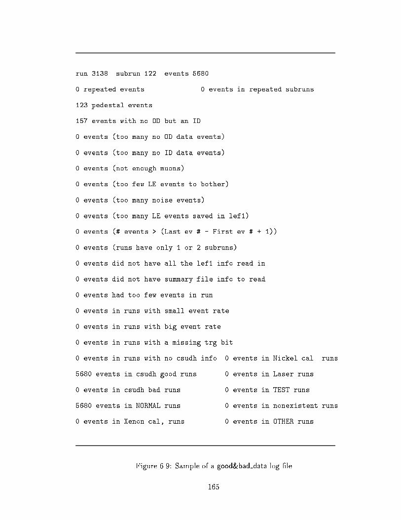
run 3138 subrun 122 events 5680
0 repeated events 0 events in repeated subruns
123 pedestal events
157 events with no OD but an ID
0 events (too many no OD data events)
0 events (too many no ID data events)
0 events (not enough muons)
0 events (too few LE events to bother)
0 events (too many noise events)
0 events (too many LE events saved in lef1)
0 events (# events > (Last ev # - First ev # + 1))
0 events (runs have only 1 or 2 subruns)
0 events did not have all the lef1 info read in
0 events did not have summary file info to read
0 events had too few events in run
0 events in runs with small event rate
0 events in runs with big event rate
0 events in runs with a missing trg bit
0 events in runs with no csudh info 0 events in Nickel cal. runs
5680 events in csudh good runs 0 events in Laser runs
0 events in csudh bad runs 0 events in TEST runs
5680 events in NORMAL runs 0 events in nonexistent runs
0 events in Xenon cal, runs 0 events in OTHER runs
Figure 6.9: Sample of a good&bad data log �le
165

algorithm.
The algorithm used for event classi�cation is basically a series of questions that
are answered by the lef2 program. Once the answer to a question is \yes", then
the event is �nished being classi�ed by lef2 and the next event is tested. Events
can be \saved" or \tossed" by lef2, just as with lef1. \Tossed" events have
negative classes and their PMT data removed, but everything else (headers, �ts,
�lter information) is saved. Table 5.2 shows the numerical values for the event
classes assigned by lef2. A description of the information saved into the data �le
by lef2 is given in Appendix A. As with lef1, a log �le is kept by lef2 to record the
number of events in each class found for every subrun processed (tape#.lef2.�ltlog).
A portion of a lef2 log �le is shown in Figure 6.10. A `tag' mode of operation
exists for lef2 and is controlled by the LE FILTER2 TAG environment variable
(similar to lef1, see Section 5.3). lef2 event classi�cations are given in bold font.
6.3.1 Pedestal Events
The presence of pedestal-taking periods has already been discussed (Section 5.6).
The beginning and end of each block of pedestal events has been read in from the
appropriate log �le. If the event number happens to fall within one of the event
blocks listed in the Livetime log �le, the event is tagged as a pedestal event.
6.3.2 Minimum Bias Events
The method for tagging a minimum bias event has changed from lef1. A separate
ag is set for every event ( ag = 0 if normal event, ag = 1 if lef1 called event
minimum bias). Minimum bias events are always saved in full regardless of the
event classi�cation. Only the events tagged in lef1 are categorized as minimum
166

--> Code Version 1011
--> Cuts Version 1007
--> Compilation Date 19961229
--> Filter Run Started On : 19970203
Run : 3138 Subrun : 122
5680 events in the subrun
2883 events were already thrown out by LEF1
4 events had the same classification as LEF1
123 pedestal events were found and thrown away
612 LE events were saved
586 LE events were thrown out
2 caterpillar (geiji) events were thrown out
52 LE events were considered junk
295 LE events were considered ringing events
2 huge ringing events
0 events are caused by flashers
0 muons that clip OD (dont enter the ID at all)
944 muons had their tubes tossed
82 new through muons found
19 corner clipping muons
45 multiple muons
31 stopping muons
Figure 6.10: Sample lef2 log �le
167

bias (no additional minimum bias samples saved). Allminimum bias events will
continue through the remainder of the lef2 classi�cation algorithm.
6.3.3 Caterpillar Muons
An entering muon does not always leave a nice �Cerenkov ring in the inner detector.
If the muon travels through the `dead space' between the ID and OD, the PMTs
see light entering the back of the PMT. This often causes the PMT hit pattern to
resemble a line instead of a �Cerenkov ring. Only the tubes very near the muon
track are hit, hence the line-like shape of the hits. These muons which speed down
the walls of the detector were nicknamed \caterpillar muons" based on the pattern
of the hits. In Japanese, these events are \geiji muons". Geiji-� events meet one
of the following criteria:
� lef1 class = unknown, stop-�, or exiting and Trashman tag = `cross-talk'
� lef1 class = unknown and Trashman tag = `bad mu-related junk'
� lef1 class = unknown, stop-�, or exiting and NID tubes < 200
� lef1 class = stop-� or exiting and Muboy called a No Fit
� lef1 class = unknown, Muboy called a No Fit, and only the OD triggered
� lef1 class = small non-contained
where NID tubes is the number of hit tubes in the inner detector. The justi�cation
for these requirements is simply that the events classi�ed as geiji-� really looked
like caterpillar muons from the event display. The last requirement is present for
the events which \fell through" lef1 without being classi�ed more exactly (signal
was present in the OD, but it did not meet the stop-� or exiting event conditions).
168

6.3.4 Big Ringing Events
After energetic muons hit the detector, the inner detector often `rings'. This `ring-
ing' creates triggers; the events look almost like an `echo' of the muon hit pattern.
Sometimes `ringing' events have a lot of ID PMT hits. Events that lef2 classi�es
as big ringing events have passed one of the tests:
� lef1 class = multi-� and Trashman tag = `ringing'
� lef1 class = multi-� and �tprev muon < 20�s
� lef1 class = unknown, �tprev muon < 20�s, and NID tubes > 500
� lef1 class = unknown, Trashman tag = `ringing', and NID tubes > 500
� lef1 class = big contained, Trashman tag = `ringing', and NID tubes > 500
� lef1 class = saved low energy and NID tubes > 200
Note that �tprev muon is the time between the current event and the previous muon
event and NID tubes is the number of hit tubes in the inner detector. By looking at
the event display and the classi�cation, these criteria are reasonable.
6.3.5 OD Clipping Muons
Sometimes a muon which enters and exits the outer detector will barely touch (or
not touch at all) the inner detector. These OD clipping muons will produce lots
of light in the outer detector while the inner detector will only have PMT noise.
To �nd these events, lef2 considers only those events which lef1 classi�ed as
unknown. If the event has < 30 ID hits occurring in any 200 ns time window and
> 20 OD hits in 200 ns, the event is called an OD clipper. An event can also be
considered an OD clipper if too many of the ID hits in the 200 ns window have
negative charge (Nnegative q in 200 ns > 0:03�NID tubes ) in addition to the > 20 OD
hits in 200 ns.
169

6.3.6 Fittable Muon Events
All high energy (NID tubes > 200) events which are not yet classi�ed by lef2 and
still have PMT data need to be identi�ed and have the track �ts performed. This
task is accomplished by Muboy (see Section 6.5). Muboy will decide if the event has
one track or multiple tracks. When the event is caused by a single track, Muboy
looks to see if the track stopped in the detector or exited. SinceMuboy is a full track
�tter, the track direction and entry points of each track are returned. When Muboy
has no problem �tting and identifying the event, the Muboy event type (in slant
type) is used as the lef2 class (thru-�, stop-�, multi-�, and corner clipper).
Sometimes,Muboy will fail and will call the event a No Fit. In this case, the event
needs to be classi�ed as what may have caused the trigger. The categorization of
these events was already described in the sections about each lef2 `junk' class.
6.3.7 LE Ringing Events
We know from scanning the saved low energy events out of lef1 that many of the
events following a muon are `ringing' events. We also know that in addition to the
bogus electronics triggers, we expect sometimes to get a real electron event after a
muon. Stopping muons which decay in the inner detector should have `good' low
energy triggers after them corresponding to the decay (Michel) electrons. Although
Michel electrons are a valuable calibration source (see Section 3.3.3), we do not want
them in the solar neutrino sample. The Michel electrons are therefore classi�ed as
LE ringing events along with the junk triggers. The LE ringing events must
meet one of these requirements:
� lef1 class = unknown, Trashman tag = `ringing', and NID tubes � 500
� lef1 class = big contained, Trashman tag = `ringing', and NID tubes � 500
� lef1 class = unknown, �tprev muon < 20�s, and NID tubes � 500
170

� lef1 class = saved low energy and �tprev muon < 20�s
� lef1 class = saved low energy and > 20 hits from the OD
in a 200 ns coincidence window (should not normally happen)
where NID tubes is the number of inner detector hit tubes and �tprev muon is the time
di�erence between the current event and the previous muon.
6.3.8 LE Junk Events
The LE junk classi�cation is intended for `trash' events which lef1 thought were
good low energy events and which are not closely associated with a previous muon.
Most of the `junk' events have been tagged by Trashman, but since Trashman is
conservative not all the junk is tagged. If an event meets one of the following
criteria, it is called LE junk.
� lef1 class = saved low energy and Trashman tag = `cross-talk', `ringing', or
`bad mu-related junk'
� lef1 class = saved low energy and Nnegative q in 200 ns > 0:03 �NID tubes
The last requirement looks for events with too many \in time" ID hits with negative
charge (negative apparent charge is caused by QAC pedestal shifts). From looking
at the events on the event display, these criteria do indeed identify event which look
like junk. We are not quite sure why the last criteria is needed, but it works.
6.3.9 Low Energy Events
Saved low energy events from lef1 which are not classi�ed as LE ringing or
LE junk, are presumed to be \good" events. The next step for these events is
the precision vertex �tter. Combo�t (described in Section 6.4) is given Hayai's �t
results as a starting point. The �tter is instructed to use in \direction only" mode
171

to �nd a good initial track direction. Combo�t then runs in \vertex and direction"
mode to �t the precise vertex and direction for the event. A cut is made using
the new �t vertex which corresponds to a 22.5 kton �ducial volume. Events with
Dwall � 2 meter are denoted saved low energy events while the rest are tossed
low energy events. Tighter �ducial volume cuts are made later in the analysis if
desired.
6.4 ComboFit Precision Vertex Fitter
Hayai quickly �gured out a reasonably good vertex for the low energy events. A
more accurate determination of the event vertex can still be performed. Combo�t
was designed for just that task. Combo�t also �gures out what direction the particle
was pointed when the �Cerenkov light was emitted. Since it is an algorithm bent on
precision, Combo�t requires a decent starting vertex and a starting direction. Com-
bo�t operates in two di�erent modes: \direction only" and \vertex and direction".
When in \direction only" mode, the best �tting direction vector is found using the
input (starting) vertex. For \vertex and direction" mode, the best �tting vertex
and direction are found by adjusting both the vertex and direction away from the
starting values. The typical procedure followed for �tting the vertex of low energy
events is to: run Hayai, run Combo�t in \direction only" mode, and run Combo�t
in \vertex and direction" mode.
The �rst thing Combo�t does is to pick which tubes will be used for the �t based
on the PMT timing. The following requirement must be met in order for the ith
PMT to be used in the �t:
jti � Tstart � dstart
vgroupj < Tcut (6.1)
172

where ti is the time of the ith PMT, Tstart is the time component of the starting
vertex, dstart is the distance between the ith PMT and the starting vertex (Xstart,
Ystart, Zstart, Tstart), vgroup =c
1:39is the group velocity in cm/ns, and Tcut = 15 ns
is the value of the cut on the time residuals. This timing cut leaves Nintime tubes
to be used in the �t.
Combo�t minimizes a �2 function with the AMOEBA routine from Numerical
Recipes [68]. AMOEBA uses the simplex method to \ooze" its way down from the
starting point into the global minimum. For an n parameter �t, AMOEBA uses an
n+1�n-dimensional simplex (a n+1�n matrix). The simplex can be thought of
as having n arms that stick out in n dimensions from a central point. Each row of
the simplex (center point or an arm) corresponds to a set of the �tting parameters.
AMOEBA needs to be given a `characteristic length' for each of the n dimensions,
so that it knows the typical range for the parameters. The � vector holds this
`characteristic length' of each of the n arms of the simplex. The simplex must be
initialized before it is given to AMOEBA; each arm of the simplex extends from the
computed starting �t parameters into only one dimension a distance equal to the
`characteristic length' for that dimension. The global minimum has been reached
when the fractional change in �2 across the arms of the simplex is smaller than the
tolerance requested. Once the global minimum has been found, it is often a good
idea to feed the minimum back into AMOEBA with a slightly lower tolerance and
verify that the global minimum has indeed been reached.
The �2 used by Combo�t may be composed of two components: timing and
pattern. The precise makeup of �2 depends on the operating mode of Combo�t.
173

The timing �2 is given by:
�2timing =PNintime
i=1
��i�i
�2j�ij = MIN(jti � T � D
vgroupj; 2�i)
�i = MIN( 3:0pqi; 0:3) ns
(6.2)
where �i is the timing residual for the ith tube, (X, Y , Z, T ) is the current ver-
tex, D is the distance from the current vertex to the ith PMT, vgroup is the group
velocity of the �Cerenkov light ( c1:39
), �i is the uncertainty in the measured time for
the ith tube, and qi is the charge for the ith tube. To keep the vertex inside the
inner detector, if the vertex is outside the black sheet layer, �2timing = 1020.
The pattern �2 can be described by:
�2pattern =PNintime
i=1
���i�
�2��i = MIN(�i � 42�; 2�)
cos �i = ~d � ~Rvertex�~Ri
j~Rvertex�~Rij
(6.3)
with �i as the angle between the �t direction ~d and the direction from vertex (X,
Y , Z) to the ith PMT and � as the uncertainty in the angle. The remainder of the
Combo�t algorithm depends on the operating mode and will be described separately
for each mode of operation.
6.4.1 \Direction Only" Algorithm
Combo�t loops through the main body of the algorithm twice. First, AMOEBA is
given the simplex centered on the given initial direction vector. Then AMOEBA
gets re-started with the simplex centered on the �rst iteration's minimum and a
tolerance smaller by a factor of 10. The basic parameters which control the detailed
behavior of Combo�t are given in Table 6.3. The �nal direction from the second
loop, (dxbest, dybest, dzbest), is the best direction found and is returned by Combo�t.
174
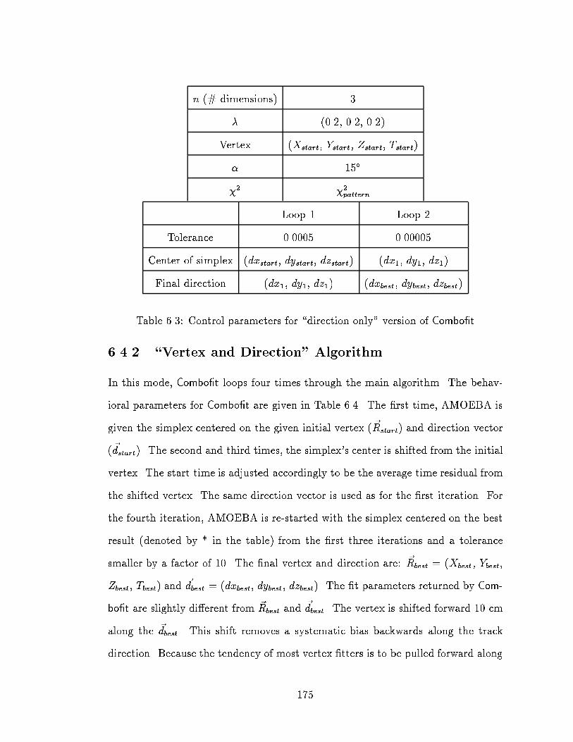
n (# dimensions) 3
� (0.2, 0.2, 0.2)
Vertex (Xstart, Ystart, Zstart, Tstart)
� 15�
�2 �2pattern
Loop 1 Loop 2
Tolerance 0.0005 0.00005
Center of simplex (dxstart, dystart, dzstart) (dx1, dy1, dz1)
Final direction (dx1, dy1, dz1) (dxbest, dybest, dzbest)
Table 6.3: Control parameters for \direction only" version of Combo�t
6.4.2 \Vertex and Direction" Algorithm
In this mode, Combo�t loops four times through the main algorithm. The behav-
ioral parameters for Combo�t are given in Table 6.4. The �rst time, AMOEBA is
given the simplex centered on the given initial vertex (~Rstart) and direction vector
(~dstart). The second and third times, the simplex's center is shifted from the initial
vertex. The start time is adjusted accordingly to be the average time residual from
the shifted vertex. The same direction vector is used as for the �rst iteration. For
the fourth iteration, AMOEBA is re-started with the simplex centered on the best
result (denoted by * in the table) from the �rst three iterations and a tolerance
smaller by a factor of 10. The �nal vertex and direction are: ~Rbest = (Xbest, Ybest,
Zbest, Tbest) and ~dbest = (dxbest, dybest, dzbest). The �t parameters returned by Com-
bo�t are slightly di�erent from ~Rbest and ~dbest. The vertex is shifted forward 10 cm
along the ~dbest. This shift removes a systematic bias backwards along the track
direction. Because the tendency of most vertex �tters is to be pulled forward along
175

n (# dimensions) 7
� (0.2, 0.2, 0.2, 15 cm, 15 cm, 15 cm, 0.1 ns)
� 20�
�2 �2timing + �2pattern
Loop 1 Loop 2
Tolerance 0.001 0.001
Center of simplex ~dstart, ~Rstart~dstart, ~Rstart � (1 m� ~dstart)
Final parameters ~d1, ~R1~d2, ~R2
Loop 3 Loop 4
Tolerance 0.001 0.0001
Center of simplex ~dstart, ~Rstart � (2 m� ~dstart) ~dstart, ~R�
Final parameters ~d3, ~R3~dbest, ~Rbest
Table 6.4: Control parameters for \vertex and direction" version of Combo�t
the track, we designed Combo�t to try several starting points by taking steps back-
wards. These backwards steps taken by the starting position for the second and
third iterations help to improve the vertex resolution of Combo�t, but the resultant
�t vertices have a slight backward bias. The 10 cm shift forward removes this bias.
6.4.3 Performance
Combo�t runs at �30 events per second running on a 333 MHz Alpha workstation.
Since Combo�t's �t is our �nal attempt at locating the Low Energy vertex and
the track direction, we need to understand the resultant �ts very well. We studied
Combo�t with the same yardsticks as Hayai (see Section 5.4.2).
176

Table 6.5 contains the Gaussian widths (�Combo�t) and total vertex errors (RCombo�t)
obtained from running Combo�t on Monte Carlo events. Samples of 10,000 MC elec-
trons were generated at several locations (X = 0, Y = 0, Z given in table) with
random directions. The three di�erent locations in the tank are representative of
the detector center, within 1 m of the edge of the 11.7 kton �ducial volume, and
the edge of the 22.5 kton volume.
�Combo�t (1-dim) RCombo�t (3-dim)
Energy Z = 0 Z = 12 m Z = 16 m Z = 0 Z = 12 m Z = 16 m
(MeV) (cm) (cm) (cm) (cm) (cm) (cm)
5 67 59 59 140 120 145
7 53 52 52 100 105 115
10 42 43 42 80 80 85
Table 6.5: 1-d and 3-d vertex resolutions of Combo�t using MC electrons
Table 6.6 gives the angular resolution (�) of the Combo�t direction for the above
sets of electron events. The angular resolution is de�ned such that 68% of the
events have �t directions closer to the true direction than the angular resolution:
~dfit � ~dtrue = cos # > cos �. Note that the position dependence of � is non-negligible
only at the lowest energies, where the vertex is least accurate. The angular reso-
lution of a water �Cerenkov detector can not get much better than what Combo�t
has already achieved. Multiple Coulomb scattering (MCS) of the electrons in water
limits the angular resolution. The average scattering angle for MCS is shown in
Figure 4.4. Direction reconstruction algorithms will not be able to achieve angular
accuracies much better than the average MCS angle.
177

Angular Resolution
Energy Z = 0 Z = 12 m Z = 16 m
(MeV) (�) (�) (�)
5 31 35 40
7 40 40 40
10 24 24 27
Table 6.6: Angular resolution of Combo�t using Monte Carlo electron events
Table 6.7 compares the �Combo�t from nickel data and a simulated nickel source.
Points with a * are outside the �ducial volume. The Monte Carlo nickel events
systematically yield Combo�t coordinate distributions which are 4 cm wider than
the nickel data.
Table 6.8 compares the 3-dimensional resolution RCombo�t for LINAC data and
MC electrons. The MC electrons were simulated as a point source located at the
end of the beam pipe, (-12.3 m, -0.70 m, 12.3 m), with directions straight down.
The MC electrons were simulated as a point source located at the end of the beam
pipe with directions pointed straight down. For the LINAC data and Monte Carlo
alike, the X and Y coordinate distributions are symmetric and very well �t (small
Gaussian widths). The Z coordinate on the other hand is much wider and asym-
metric. For this reason, we give only RCombo�t.
178

Nickel Source
Source Position �Combo�t Data �Combo�t MC
(cm) (cm) (cm)
(35, -70, 0) 49 52
(35, -70, 1200) 46 53
(35, -70, 1600) 45 49
(35, -1200, -1200) 47 48
(35, -1200, 0) 46 50
(35, -1555, -1200) * 45 50
(35, -1555, 0) * 45 50
Table 6.7: Gaussian widths from Combo�t on nickel data and MC
LINAC
Beam Energy RCombo�t Data RCombo�t MC
(MeV) (cm) (cm)
5.866 150 150
6.782 120 125
8.637 100 105
15.923 60 70
Table 6.8: Total vertex errors from Combo�t on LINAC data and MC
179

6.4.4 E�ect of Dwall � 2 meters Cut
Since lef2 makes a �ducial volume cut based on the Combo�t vertex, the e�ciency
for saving the solar neutrino events inside the �ducial volume should be studied.
We do this by studying the energy dependence of the the e�ciency �1:
�1 =# of events which have Dwall[fit] � 2 meter
# of events generated with Dwall[MC] � 2 meter
This e�ciency is shown in Figure 6.11. The Monte Carlo events were generated all
the way up to the inner detector wall. Events with generated vertices outside the
�ducial volume may �t inside the �ducial volume, thereby increasing the observed
e�ciency for saving events. There is some slight energy dependence which is due
to the �tter resolution as a function of electron energy.
Generated Electron Total Energy (MeV)
ε1 fo
r C
ombo
fit (
%)
Figure 6.11: � of Dwall � 2 meter cut on Combo�t vertex using MC electrons
180

6.5 Muboy Track Fitter
lef2 needs routines which can perform track �ts for multiple muon, stopping muon,
and through-going muon events which may not have OD data. Muboy3 is all these
rolled into one neat package. Muboy determines if an event was produced by a
single track or multiple (parallel) tracks in the inner detector. If it is a single
track event, Muboy looks to see if it stopped in the ID (the OD is used also if it
exists). An event classi�cation is returned with the �tted track parameters; the
di�erent classi�cations are: No Fit, Thru Mu, Stop Mu, Multi Mu1, Multi Mu2,
or Corner Clipper. The Multi Mu1 and Multi Mu2 classes both indicate multiple
muon events, just identi�ed with di�erent algorithms. Corner Clipper events are
usually through-going muons which just clip a corner of the ID. They are tagged
di�erently from the rest of the Thru Mus since the �t direction is not very reliable.
6.5.1 Algorithm
Before Muboy starts trying to �t the event, it selects out the PMT hits which will
be used for the �t. All used inner detector PMT hits must pass a charge cut (given
in Table 6.9) which depends on the number of hit ID tubes in the event (NID tubes).
Tubes which pass the charge cut are subjected to the nearest neighbor cut. Each
used ID tube is required to have at least Nnn adjacent PMTs hit within 10 ns. Ta-
ble 6.10 shows the values for Nnn as a function of the total number of hit ID tubes.
The �nal number of \good" ID tubes is Nclean. If at any point in the algorithm
Nclean < 10 hits then the event is called a No Fit and Muboy stops working with
that event. The only cleaning applied to the OD hits is that the tubes used must
have a positive charge.
3Muboy was developed by Bob Svoboda.
181

NID tubes Minimum charge in ID tube
>10,000 3.0 pe
8,000 - 10,000 2.5 pe
<8,000 2.0 pe
Table 6.9: Minimum charge requirements for ID tubes used in Muboy �t
NID tubes Minimum value of Nnn
>7,500 5 tubes
5,000 - 7,500 4 tubes
2,500 - 5,000 3 tubes
500 - 2,500 2 tubes
<500 1 tube
Table 6.10: Nearest neighbor requirement for ID tubes used in Muboy �t
182

Muboy �gures out moderately reasonable guesses for an entry point and track
direction before it can �nd the `best' track. The starting entry point is found by
selecting the earliest PMT which has 3 nearest neighbors. If no tube meets this
criterion, the required number of nearest neighbors is reduced one at a time until
an entry point candidate tube is located. The entry position is the coordinates of
the early tube; the entry time is the time of the tube hit. The �rst guess at an
exit point is the center of the `mini-patch' of 9 tubes (1 tube and its 8 surrounding
neighbors) which contains the most charge. A line drawn between the entry and
exit yields a starting direction for the track.
To reduce the noise much further around the entry point, a `causality' cut is
made to the tubes. We know that if a muon enters the ID at the entry point/time,
then PMT hits which are produced by \direct" light from the muon (light which
is not scattered) can not be hit earlier than the travel time of the muon: Tentry +
dentry pmt
v1where dentry pmt is the distance from the entry point to the hit tube and
v1 is the muon speed. If there are multiple particles in the detector simultaneously,
there maybe some of these `early' PMT hits. The hits can not be hit later than
the travel time of light in the water: Tentry +dentry pmt
v2where v2 is the speed of
light in water. Light which scattered in the detector will occur late. Light from
other tracks in a multi-track event can be early or late. Muboy allows the maxi-
mum and minimum speeds to be a bit farther apart so the `causality' cut is not
too stringent: v1 = 34:0 cm/ns and v2 = 18:0 cm/ns. Multiple muon events can be
recognized because they often have a lot of hits which occur `earlier' than causality
allows. For this reason, Muboy counts the number of tubes Nearly which appear
to be hit at speeds faster then 33 cm/ns. If Nearly > 45, the event is called a
Multi Mu1 event. For these events, the causality cut is tightened to remove even
183

more of the hits induced by the other tracks: v1 = 32:0 cm/ns and v2 = 19:5 cm/ns.
Muboy maximizes a `goodness of �t' (GOF) parameter. The GOF is de�ned as:
GOF = F (fcone)NcleanXi=1
g(�ti) (6.4)
where F is a function of the fraction of hits in the �Cerenkov cone (fcone), g is a
function of the the time residual �ti = Texpected� ti, ti is the measured time of tube
i, and Texpected is the calculated time at which the tube should have been hit.
Tubes are considered `in the �Cerenkov cone' if either of these conditions are
met: �~Rpmt�~Rentry
j~Rpmt�~Rentryj
�� ~dtrack > 0:74
OR
j~Rpmt � ~Rentry j < 2 m
(6.5)
Once it is known which of the PMT hits are `in the cone', the fraction of hits in
the cone (fcone) can be computed. F , the pattern component to the GOF, takes
the following form:
if fcone < 0:75 then F (fcone) =0:9Ccut
fcone
if fcone > 0:75 then F (fcone) =0:1fcone+0:9�Ccut
1�Ccut
where Ccut = 0:74
(6.6)
The below two forms for g(�ti) were determined by looking at timing distributions
from the data.
if �ti < 0 or qi > 30 pe g(�ti) = exph� (�ti�tmean(qi))2
2�(qi)2
iif �ti > 0 g(�ti) = exp
h� �ti
�(qi)
iwhere �(qi) = 1:690 + 2:514 exp
h� qi
2:453
i[ns]
�(qi) = 1:254 + 14:863 exph� qi
2:316
i[ns]
(6.7)
184

The GOF is maximized by allowing the track direction to move around on a grid and
keeping the entry point and time �xed. Once the best �t track direction is found, a
second iteration is performed for all events not classi�ed as a Multi Mu1. This time
when the track direction changes, the entry time is also allowed to change; it is
calculated from the hits which occur within a 26.7 ns time residual window around
the track. A third step is to compute the GOF with a slightly di�erent pattern
component from previous calculations: Ccut = 0:65. After this second maximiza-
tion, Muboy counts the number of early hits Nearly2. If Nearly2 > 35 and the event
has not been classi�ed yet, it is called a Multi Mu2. If the event still does not have
a class, it is called a Thru Mu. Direction �tting is �nished for the Thru Mu events,
but not for the Multi Mu1s or Multi Mu2s.
All Thru Mu events with Ntubes < 2,000 are examined for the possibility of being
a through-going track which clips the corner of the ID. It is very hard to �t the
track direction well for these events due to the small lever arm of the track in the
ID. Corner clipping muons can be identi�ed by their tracks entering and exiting
the ID near the edges. If a track starts near the top corner and is heading `out'
(Xentry�dx+Yentry�dypX2entry+Y
2entry
> 0:05), the event is tagged as a Corner Clipper. If the track
comes in the bottom corner, and the distance between the entry point and the exit
point (as de�ned by the `mini-patch') is < 3 m, the event is classi�ed as a Corner
Clipper.
The remaining Thru Mu events are checked to see if they are stopping muons.
To recognize a stopping muon, Muboy looks at the charge generated by the end
of the track (and if present the OD data near the exit point). The total charge
QID exit is counted for the tubes whose positions lie within 2 m of the exit point for
185

the �tted track. The OD tubes within 4 m of the exit point (projected to the OD
PMT plane) have their charge totaled into QOD exit. An event can get classi�ed as
a Stop Mu by meeting any of the following requirements:
� QID exit < 200 pe
� QID exit < 400 pe and 0 < QOD exit < 30 pe
� QOD exit > 30 pe and QID exit < 150 pe
� no OD data and QID exit < 300 pe
Muboy is �nished with events which are still classi�ed as Thru Mu. Events called
Stop Mu have the stopping point calculation as the �nal Muboy step.
To calculate the stopping point, Muboy looks at the observed energy loss via
�Cerenkov light production per unit track length, dElight
dx. This is done by looking at
the amount of detected light per unit track length. By assuming that most of the
PMT hits were induced by unscattered light from the muon track, the time of the
PMT hit is used to determine the photon emission point on the muon track. By
examining the amount of charge detected from each section of muon track, dQdet
dx, we
should be able to see the drop o� which corresponds to the end of the muon track.
The dQdet
dxof the track is histogrammed in 50 cm dx bins. The nominal dQdet
dxvalue
for the minimum ionizing portion of the track is calculated by averaging together
the �rst 3 bins in the dQdet
dxhistogram. The second consecutive bin which has dQdet
dx
fall below�dQdet
dx
�cut
is the bin which contains the stopping point. The value for�dQdet
dx
�cut
= 0:4�dQdet
dx
�nominal
is not allowed to go below 1 pe/cm.
Multiple muon events go through a second round of the above described itera-
tions. Before Muboy runs o� to do this last set of GOF maximizations, more hits
from the `other' tracks must be removed so the accuracy of the �rst track �t can
186

be improved. All hits outside a 13.3 ns timing residual window around the current
track are cut. The �rst iteration (�xed entry time) is repeated with the new set of
cleaned tubes. The second iteration is repeated using only the tubes inside a 10 ns
time residual window. Multi Mu1 and Multi Mu2 events are now �nished with the
direction �tting.
At this point in the �tting, Muboy has a direction and entry point for one of the
tracks in a multi-track event. It is assumed that the multiple muons have parallel
track directions. Entry points are needed for the rest of the tracks, once the number
of tracks is determined. To do this, Muboy wants to reverse some of the cleaning
done to the PMTs; the Nclean PMTs passing the initial charge and nearest neighbor
cuts are used. To this sample of PMT hits, a cut is applied which saves only the
hits near the beginning of the track:
~ntube � ~dtrack > 0 (6.8)
where ~ntube is the normal to the PMT and ~dtrack is the track direction. The tubes
are further selected to try and collect the tubes which are near the muon tracks.
This is done by computing the `plane wave time' tplane at which the PMT would
have been hit if the light was a plane wave traveling at speed c:
tplane = Tentry +j(~Rpmt � ~Rentry) � ~dtrackj
c(6.9)
where ~Rpmt is the PMT position vector and ~Rentry is the vector to the entry point.
If �33:3 ns < tplane � ti < 16:6 ns, the tube is kept. An event which has fewer
than 4 tubes left is said to only have 1 track (but classi�cation is still Multi Mu1
or Multi Mu2). Since the goal now is to �nd entry points for the `other' tracks,
Muboy removes the hits closely associated with the �rst track. This is done by
rejecting PMTs which have 0 < Texpected � ti < 10 ns and are within 12 m of the
187

track. Muboy iterates the following procedure until the number of remaining tubes
is <6 or until 9 tracks have been found.
1. Locate earliest hit �! this tube gives entry point and time
2. Cut tubes closer than 12 m to the track with 0 < Texpected � ti < 10 ns
3. Count number of tubes just cut �! if > 5, the track is valid
4. Count number of tubes left after cut �! if � 6 tubes, go back to (1)
Once Muboy �nished the above steps, it has calculated the track direction and
entry points for all the tracks in the Multi Mu events and is completely �nished
with multi-track events.
6.5.2 Performance
Several things about Muboy have been studied: the track resolution for each type
of event and the event identi�cation e�ciency. To compute the identi�cation e�-
ciency, the hand scanned data sample of 10, 207 events was used. No �ltering was
done to the data prior to giving all events with >200 ID PMT hits to Muboy. Ta-
ble 6.11 contains the Muboy event identi�cation results. Overall, Muboy correctly
identi�es a very large fraction of the events, including the di�cult multiple muons.
The resolution of theMuboy track �t must be studied for each type of muon sep-
arately. The entry point error (�entry) and the angular error (�dir) in the direction
�t will be given for each event type. Figure 6.12 shows the distributions of �entry
and �dir for the events which both the hand scan and Muboy called stopping muons.
Figures 6.13 and 6.14 give the same type of distributions for single through-going
muons and multiple muon events. The through-going muons were classi�ed as such
by the hand scan and Muboy. On the multiple muon events, �entry and �dir are
calculated for each track assuming that there were less than 3 tracks.
188

Hand Fits Results
Muboy class # ev. Thru-� Stopping � Multiple �
Thru-� 1728 1717 3 6
C.C. 77 74 1 0
Stop-� 113 28 57 0
Multi-� 129 17 0 112
No Fit 0 0 0 0
Table 6.11: Muboy identi�cation e�ciency for muon events taken from the data
Figure 6.12: Resolution of Muboy track �t on stopping muon events
189
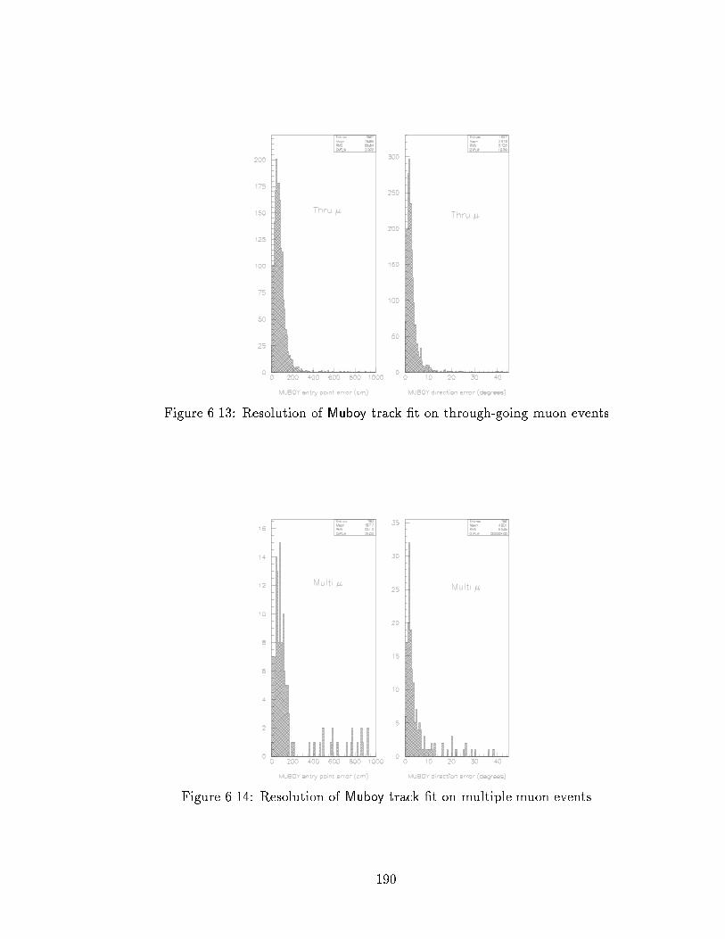
Figure 6.13: Resolution of Muboy track �t on through-going muon events
Figure 6.14: Resolution of Muboy track �t on multiple muon events
190

6.6 E�ciencies
6.6.1 Muon Identi�cation
As with lef1, the e�ciency for lef2 recognition of muon events was studied. Be-
cause lef2 is run after lef1, the e�ciency that we will compute is a combined
e�ciency of both �lters together. Table 6.12 gives the number of events of each
type found by lef2 in the hand scanned sample of 10, 207 events. Each column
has two numbers listed; Toss is the number of events with the PMT data thrown
out while Keep is the number of events with PMT data saved. The C.C. class
corresponds to corner clipper muons. All but 11 events from the hand �t sam-
ple are present in the table; the missing 11 events (10 through-going muons and 1
stopping muon) were classi�ed as geiji-�. The key piece of information contained
in the table is: the misidenti�cation probability for muon events is low.
Hand Fits Results
Thru-� Stopping � Multiple � Other
lef2 class # ev. 1836 61 117
Toss Keep Toss Keep Toss Keep All
Thru-� 1827 1690 78 10 0 48 0 1
C.C. 51 41 7 1 0 0 0 2
Stop-� 74 10 2 50 0 0 0 12
Multi-� 81 6 2 0 0 69 0 4
Table 6.12: Combined lef2 and lef1 e�ciency for muon events
191

6.6.2 Low Energy Events
We have already seen the e�ciency of the Dwall � 2 m cut on the Combo�t vertex.
The e�ciency of the lef2 �lter as a whole to save �ducial volume solar neutrino
events needs to be examined. The intention is to check the identi�cation e�ciency,
but some aspects simply can not be checked with the Monte Carlo simulated events.
For example, solar neutrinos are generated by themselves (i.e. without any muon
events thrown in), so the cuts on �tprev muon will not be mimicked. However, most
of the cuts which the Monte Carlo does not model can be accounted for by a loss in
the total live time instead of contributing to an energy-dependent e�ciency. Having
said all that, the e�ciency is calculated to be:
�1 =# of events passing lef2
# of events generated with Dwall[MC] � 2 meters(6.10)
Figure 6.15 shows �1 as a function of electron energy. The high at e�ciency is
precisely what lef2 was designed to achieve.
Generated Total Energy (MeV)
LEF
2 ef
ficie
ncy
for
F.V
. eve
nts
Figure 6.15: � of lef2 �lter on simulated electrons in 22.5 kton �ducial volume
192

6.7 Level 112
While the good run criteria was being fully developed, lef2 could not be processing
data. We wanted to use the available CPU without waiting for lef2 to be fully
ready. The two CPU-hungry processes inside lef2 are Muboy and Combo�t. lef1.5
was born to run Muboy on the relevant events, save the �t information, and throw
away PMT data for the events which Muboy could identify and �t. lef2 then reads
the output data tapes from lef1.5. It was believed that this was a safe method of
utilizing available CPU in a way which would not be `wasted' in the future. lef2
only needed minor modi�cations to accommodate lef1.5. The �rst modi�cation
was to add another lookup table for good&bad data so it could �gure out which
lef1 log �les to open based on the lef1.5 tape number. Also, lef2 checks for
the Muboy �t information in the data �le before calling Muboy. The identi�cation
algorithm for events did not change at all with the addition of lef1.5. Three lef1
tapes �t onto a single lef1.5 output tape. One output tape from lef2 holds two
lef1.5 tapes. lef1.5 is now a standard component to the Low Energy data �ltering.
193

Chapter 7
Final Data Reduction
The output of the lef2 �lter yields approximately 1 DLT tape (30 GBytes) per
month of low energy events. Still, a very small fraction of these events are real solar
neutrinos. In order to further extract the neutrino signal, we must apply physics-
based cuts to the lef2 data sample. There are several ways in which these cuts can
be made. One way is to run a `level 3' �lter program which writes out a data �le
with the events which pass the �nal cuts. The method we utilize creates NTUPLE
�les [70] with a summary of the event information. Using PAW [69], the cuts are
applied to the NTUPLE when making plots, etc. The bene�t of using NTUPLEs
and making the �nal cuts \interactively" is that the cuts can be changed at any
time without having to re-process data.
7.1 NTUPLE Program - le ntuple
A special program (called le ntuple) collects the needed information and creates
the NTUPLE �les [69]. le ntuple performs several functions:
� compute Ne�ective for every LE event
� call Cubist to tag spallation events
194

� create a log �le containing the run #, subrun #, Cubist exposure, and a \keep
or toss" ag for every subrun
� create lists of good and bad subruns
The Ne�ective calculation and Cubist are described in this Chapter. The log �le is
part of our bookkeeping system to keep track of the processed subruns.
The structure of the NTUPLE was designed to have enough information so
that most cuts could be studied and optimized. Tables 7.1 through 7.5 list all the
information contained in the NTUPLE. Some of the information is accumulated
from zebra banks (see Appendix A) such as the header bank (HEAD), the lef1
and lef2 banks, and �tter banks (COMB and HAYA). A few things (spallation
ags, energy) are the results of routines called by le ntuple which are described
in the next sections.
7.2 Sun Location
An electron undergoing neutrino-electron elastic scattering preserves the incident
neutrino direction. The directions of the solar neutrino induced events in Super-
Kamiokande therefore will correlate with the location of the Sun. In order to see
the events pointing back to the Sun, we must know where the Sun is at all times of
the day. Determining the Sun location is a fairly straightforward process, once the
coordinates of the Super-Kamiokande site and the time of day are known. Super-
Kamiokande is situated at a latitude and longitude of 36.426 degrees and 137.313
degrees respectively. The �y axis of the Super-Kamiokande coordinate system
points 49.85 degrees West of magnetic North. The GPS clock is usually used for
the time of day. Sometimes the �ber link connection from the GPS antenna to
195

Field Description
run run #
subrun subrun #
eventnum event #
trg id `trigger id'
yrmthday date event triggered (computer clock)
hrminsec time event triggered (computer clock)
Ntotal total # of ID hits
Nq<0 # of ID hits with negative charge
trash Trashman event tag
minbias minimum bias event tag
goodbad good&bad data subrun tag
�tped time (in �s) since last pedestal period
�t time (in �s) since previous trigger
Qtotal total charge in ID
Table 7.1: General event information in the Low Energy NTUPLE
196

Field Description
cubist Cubist tag
spall ag tag for spallation cuts similar to Cubist
�tnofit time (in �s) since last Muboy No Fit event
Qnofit total ID charge for the last Muboy No Fit event
classno�t lef2 class for the last Muboy No Fit event
�tgeiji time (in �s) since last geiji-� event
�todclip time (in �s) since last OD clipper event
Table 7.2: Spallation variables in the Low Energy NTUPLE
Field Description
(dxsun, dysun, dzsun) direction vector pointing to the Sun
cos �sun cosine of angle between Combo�t track direction
and (dxsun, dysun, dzsun)
clock ag for which clock was used to locate the Sun
(GPS or computer)
Table 7.3: Sun location information in the Low Energy NTUPLE
197

Field Description
Combo�t information
(Xc, Yc, Zc, Tc) vertex
(dxc, dyc, dzc) track direction
�2c chi-squared
Hayai information
(Xh, Yh, Zh, Th) vertex
GOFh Hayai goodness of �t
(dxh, dyh, dzh) anisotropy vector
Energy information
N50c N50 computed from Combo�t vertex
N50h N50 computed from Hayai vertex
Neff Ne�ective computed from Combo�t vertex
E energy of event computed from Neff
Table 7.4: Fit information in the Low Energy NTUPLE
198

Field Description
Information on each of the (�10) previousmuons within 10 s and 5 m of this event
class of ith � lef2 classi�cation
Ni total # of ID hits in � event
�ti time di�erence (in �s) since muon
Qi total ID charge in � event
�d� distance of closest approach between � track and LE vertex
Ltrack track length of muon
Table 7.5: Previous muon information in the Low Energy NTUPLE
Super-Kamiokande goes down. When this happens, the GPS time recorded in the
data corresponds to a date which is before the Super-Kamiokande detector was
operational. The GPS time is checked to see if it is later than April 1, 1996. If it
is not, we use the clock time from the online host computer which is stored in the
header.
7.3 Spallation Events
When energetic muons travel through water, they will sometimes cause oxygen
nuclei to break up. This general process, called `spallation', occurs with lots of
di�erent nuclei. The remnant pieces of the oxygen nucleus are often unstable ele-
ments like 12B and 12N. These radioactive spallation products will decay and appear
to look like contained low energy events. However, they are de�nitely not solar
neutrino-induced events. Spallation products form a signi�cant contribution to the
solar neutrino background.
199

To remove the spallation events from the solar neutrino sample, we want to
make cuts based on the positional correlation between the low energy vertex and
the muon track and time correlation between the muon and low energy events.
Historically, spallation events are removed by cutting the low energy events within
a certain time of the muon which have vertices inside of a cylindrical volume around
the muon track. Figure 7.1 shows pictorially a typical spallation cut around a muon
track.
cutR
∆ Tmuon track for a time
Cylinder cut around
Muon TrackTo Remove Spallation Events
Figure 7.1: Cylinder cut around a muon track to remove spallation events
7.3.1 Characterization
The spallation-induced events in our lef1 data sample have been studied in great
detail1. The goals of this investigation were to characterize the time scales, ex-
plain the possible source isotopes, and calculate the event rates of the spallation
events. The results of this characterization study will be given. The optimization of
1This spallation study was completed by Bob Svoboda.
200

the speci�c `spallation' cuts made to the �nal data sample will then be summarized.
In order to see correlations between the muon and low energy events, a running
history of the muon events in the past minute is kept. The track �t parameters
come from FSTMU and MUBOY while Hayai gives the low energy vertex position
(The tuning of Combo�t was not �nished when this work was done.). The important
parameters for the characterization of spallation events are:
�T Time between the LE event and the previous muon event
�D Distance of closest approach by the muon track to the LE vertex
NID tubes Total number of ID tubes (to check the approximate energy)
1 ms Time Scale
An exponential decay with a half-life of �100 �s (di�cult to �t well) is seen in the
time di�erence between low energy (LE) events and muon events (see Figure 7.2).
The correlation distance (�D) between the LE event vertex and the muon track
is shown in Figure 7.3. The two horizontal scales are �D and its square. The
non-spallation events should yield a at (�D)2 distribution. The sharp peak in
the (�D)2 distribution is the spallation events. The �D distribution may be a
little more intuitive, but the spallation peak is harder to identify because of the low
statistics and the shape of the background. The distribution of the number of ID
PMT hits shows a clear bump for the events with vertices within 3 m of the muon
track and time di�erences <1 ms (Figure 7.4). The NID tubes bump falls o� above
�10 MeV (very coarse estimate). The number of hits does not appear correlated
with the charge deposition of the muon, which is expected of `ringing' events. No
candidate � decay sources were found in the Table of Isotopes [71] with this end
point energy and half-life. All listed isotopes that could be created from oxygen
201
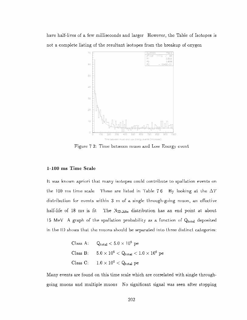
have half-lives of a few milliseconds and larger. However, the Table of Isotopes is
not a complete listing of the resultant isotopes from the breakup of oxygen.
Figure 7.2: Time between muon and Low Energy event
1-100 ms Time Scale
It was known apriori that many isotopes could contribute to spallation events on
the 100 ms time scale. These are listed in Table 7.6. By looking at the �T
distribution for events within 3 m of a single through-going muon, an e�ective
half-life of 18 ms is �t. The NID hits distribution has an end point at about
15 MeV. A graph of the spallation probability as a function of Qtotal deposited
in the ID shows that the muons should be separated into three distinct categories:
Class A: Qtotal < 5:0� 105 pe
Class B: 5:0� 105 < Qtotal < 1:0 � 106 pe
Class C: 1:0� 106 < Qtotal pe
Many events are found on this time scale which are correlated with single through-
going muons and multiple muons. No signi�cant signal was seen after stopping
202

Figure 7.3: Correlation between LE vertex and muon track
Figure 7.4: Total number of ID hits for events correlated with a previous �
203

muons. Also, a fairly high rate of events was found for Muboy No Fit events which
had >500 pe in the inner detector. For these No Fit events a global veto must be
done - since there is no muon track to correlate with the LE vertex.
Isotope Half-Life Energy Branching Ratio
11Li 8.5 ms E� =20.6 MeV 39%
E� =11-19 MeV 60%
13O 8.6 ms E� =16.7 MeV 89%
15B 10.5 ms E� =18.0 MeV 100%
12N 11.0 ms E� =17.3 MeV 95%
14B 13.8 ms E� =14.5 MeV E =6.1 MeV 82%
13B 17.4 ms E� =13.4 MeV 92%
12B 20.2 ms E� =13.4 MeV 97%
12Be 23.6 ms E� =11.7 MeV 100%
Table 7.6: Isotopes with half-lives between 1-100 ms
100-600 ms Time Scale
In this time regime, the �T distribution for events within 2 m of a through-going
muon track �ts well to an exponential decay with an e�ective half-life of 0.11 s -
indicating that spallation events are de�nitely being observed. The �T distribution
for events between 2 and 3 m of the track is at. No spallation is discernible from
stopping muons. After multiple muons events with more than 6 tracks, the �T
distribution also �ts well to a 0.11 s half-life. Table 7.7 shows the few isotopes
listed in the Table of Isotopes which can contribute to spallation on this time scale.
204

Isotope Half-Life Energy Branching Ratio
8He 0.119 s E� =10.7 MeV 84%
9C 0.127 s E� =4.4-16.5 MeV
9Li 0.178 s E� =13.6 MeV 50%
E� =11.2 MeV E =2.4 MeV 34%
Table 7.7: Isotopes with half-lives between 100-600 ms
0.6-5 s Time Scale
With this time scale, the \natural" time scale due to the trigger rate comes into
play. Even though the average time between triggers is 0.1 s, the average time
between events which are within a few meters of a muon event is much longer.
The \natural" fall-o� must be removed from the �T distribution before �tting for
the e�ective half-life of 0.9 s. The rate from multiple muon events with �4 tracksand the rate after Muboy No Fit events are di�cult to see due to a limitation in
the analysis program used for this study. Previous time scales showed that the
spallation rates from two categories of multiple muon events were comparable; it is
assumed that the same is true for this time scale also. No track-related events are
apparent after stopping muons. Isotopes that may cause the observed events are
given in Table 7.8.
5-70 s Time Scale
The isotopes with half-lives between 5 and 70 s are listed in Table 7.9. Production
of 16N occurs when a stopped �� is captured by the oxygen nucleus, which is not
strictly speaking spallation. To remove 16N events (and any other event which is
correlated with a muon stopping point), a spherical volume centered on the stopping
205

Isotope Half-Life Energy Branching Ratio
16C !15N� 0.747 s E� =5 MeV E =3 MeV 84%
Eneutron =3.35 MeV
8B 0.770 s E� =18 MeV 100%
8Li 0.838 s E� =16 MeV 100%
15C 2.45 s E� =9.8 MeV 37%
E� =4.5 MeV E =5.3 63%
Table 7.8: Isotopes with half-lives between 0.6-5 s
point is cut. Because of the low end point energy, the 14O decay will become
more important as Super-Kamiokande continues to take data and lower the energy
threshold. With this long time scale, it is di�cult to separate the spallation �T
decay from the \natural" fall-o� with the present analysis. The optimization of a
cut on this time scale will need to be performed using di�erent analysis tools.
Isotope Half-Life Energy Branching Ratio
16N 7.13 s E =6.13 MeV E� =4.3 MeV 66%
11Be 13.8 s E� =11.5 MeV 55%
E� =9.4 MeV, E =2.1 MeV 31%
10C 19.3 s E� =2.9 MeV 99%
14O 70.6 s E� =2.6 MeV E =2.3 MeV
Table 7.9: Isotopes with half-lives between 5-70 s
206

Spallation Rate
All these time scales, muon categories, and track correlation distances can become
a bit confusing. It is di�cult to �gure out which muon type and time scale gen-
erates the most spallation events. Obviously, the modes which produce the most
background events deserve to have the most attention when the cuts are tuned.
Table 7.10 gives the rate estimates from this study for each spallation mode. These
rates were calculated from the �D distributions using the �t half-life time to the
�T distribution. Using all time scales and all muon events, the total spallation
rate is �600 events/day.
Event Type
Time Thru � Multiple � Stopping � Muboy No Fit
<4 tracks �4 tracks1 ms 8-14 3-5 16-27
100 ms 153 18 19 - 105
600 ms 34 6 4 - 10
5 s 96 14 14 - none ?
70 s 64 8 8 none ? none ?
TOTAL 355-361 evday
94-96 evday
131-142 evday
Table 7.10: Measured spallation rates in events per day
7.3.2 Cut Optimization
We need to remove as many of the possible spallation events as we can from the
solar neutrino data sample. This can obviously be done most simply by cutting out
the entire detector for a certain amount of time after a muon event. This simplis-
207
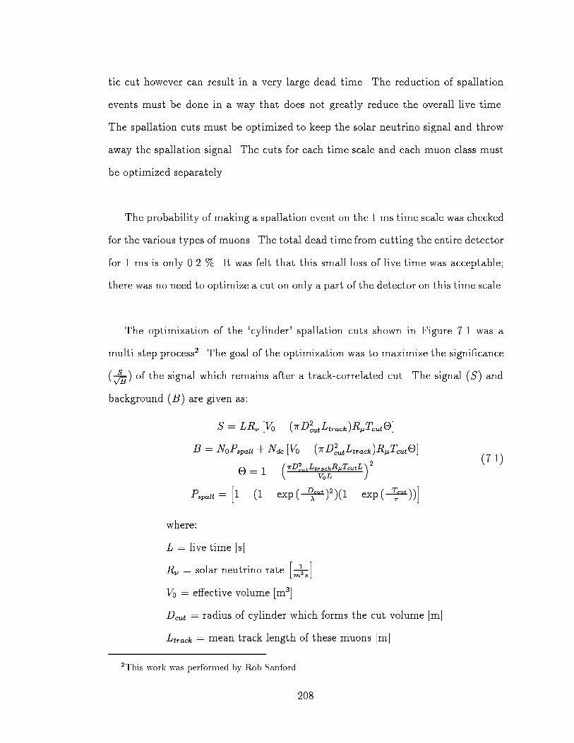
tic cut however can result in a very large dead time. The reduction of spallation
events must be done in a way that does not greatly reduce the overall live time.
The spallation cuts must be optimized to keep the solar neutrino signal and throw
away the spallation signal. The cuts for each time scale and each muon class must
be optimized separately.
The probability of making a spallation event on the 1 ms time scale was checked
for the various types of muons. The total dead time from cutting the entire detector
for 1 ms is only 0.2 %. It was felt that this small loss of live time was acceptable;
there was no need to optimize a cut on only a part of the detector on this time scale.
The optimization of the `cylinder' spallation cuts shown in Figure 7.1 was a
multi-step process2. The goal of the optimization was to maximize the signi�cance
( SpB) of the signal which remains after a track-correlated cut. The signal (S) and
background (B) are given as:
S = LR� [V0 � (�D2cutLtrack)R�Tcut�]
B = N0Pspall +Ndc [V0 � (�D2cutLtrack)R�Tcut�]
� = 1 ���D2
cutLtrackR�TcutL
V0L
�2Pspall =
h1� (1� exp (�Dcut
�)2)(1 � exp (�Tcut
�))i
(7.1)
where:
L = live time [s]
R� = solar neutrino rateh
1m3s
iV0 = e�ective volume [m3]
Dcut = radius of cylinder which forms the cut volume [m]
Ltrack = mean track length of these muons [m]
2This work was performed by Rob Sanford.
208
R� = muon rate for this class of muon [1/s]
Tcut = length of time to hold the cylinder cut of radius Dcut [s]
� = non-overlap fraction
N0 = spallation rateh1m3
iPspall = probability of being spallation
� = characteristic distance from track [m]
� = characteristic time scale [s]
Ndc = dc background levelh1m3
i
When overall constants are ignored, the equation for SpBends up being independent
of R� and L. The values for R�, Ltrack, �, � , andNdc
N0are all taken from the data.
Using this equation for SpB, the values of Dcut and Tcut are optimized for each
muon class (with a track �t) and time scale. This optimization is done successively,
meaning that the best cut values for longer time scales will depend on the results
from the shorter times. The �nal cuts used in this analysis are given in Table 7.11.
7.3.3 Cubist
The loss in detector exposure (volume � live time) from making these `cylinder
cuts' must be accounted. One can think of the total exposure after spallation cuts
as an e�ective (smaller) livetime times the full �ducial volume. An e�ective livetime
for the 22.5 kton �ducial volume (corresponding to Dwall � 2 m) can be computed
with varying degrees of accuracy. One of the di�culties in getting an accurate
measure of the e�ective livetime is overlapping muon tracks. For a particular set
of cuts, the exposure lost by the `cylinder' cut (�cut) would be:
�cut = �R2cutLtrack�Tcut (7.2)
209

Event Type Time Cut Distance Cut Spall ag
any muon 1 ms globalp
any muon 120 ms Rcylinder = 3 mp
Muboy No Fit 100 ms global -
Muboy No Fit Qtotal < 500 pe 1 ms global -
stopping � 10 s Rcylinder = 1:5 mp
stopping � 30 s Rsphere = 1:5 mp
thru � Class A 0.5 s Rcylinder = 2:2 mp
thru � Class A 4.0 s Rcylinder = 1:2 mp
thru � Class A 10 s Rcylinder = 0:6 mp
thru � Class B 0.8 s Rcylinder = 3:0 mp
thru � Class B 7.5 s Rcylinder = 3:0 mp
thru � Class B 50 s Rcylinder = 0:8 mp
thru � Class C 0.6 s Rcylinder = 3:0 mp
thru � Class C 6.5 s Rcylinder = 2:8 mp
thru � Class C 25 s Rcylinder = 1:6 mp
multiple � <6 tracks 100 ms globalp
multiple � �6 tracks 3 s global -
multiple � <3 tracks 10 s Rcylinder = 2:5 mp
multiple � <3 tracks 30 s Rcylinder = 1:5 mp
Total dead time =�12%
Table 7.11: Spallation cuts used in analysis
210

where Rcut is the maximum perpendicular distance from the track for a `cut' low
energy vertex, Ltrack is the track length of the muon, �Tcut is the length of time
time after the muon for which events are cut. This equation assumes the most
simplistic type of track - one which is perpendicular to the tank walls on entry and
exit. This con�guration does not happen often. Usually the tracks are not normal
to the walls and the cut exposure becomes more complicated. The equation for �cut
becomes more complicated still if the muon track scrapes a wall such that the full
cylindrical volume does not lie in the inner detector. If two muon tracks are close
enough that the `cut' regions overlap, the loss in exposure is not �cut1 + �cut2 . It is
actually smaller by an amount which depends on the volume of the overlap region.
It is di�cult to accurately account for these overlaps analytically. A method of
tagging the spallation events and accurately computing the total exposure of the
detector was needed.
Cubist 3 solves the problem of determining the detector exposure after spallation
cuts. Inside Cubist, the volume of the inner detector is broken up into 22803 \cubes"
which each take up 1 m3. Each cube has an \alarm clock" which is \set" when
a muon passes near the cube (or when a global veto is on). The timers on the
alarm clocks run down as the event times progress forward. While the timer on
a particular cube's alarm clock is non-zero, any low energy event with a vertex in
the cube is tagged as a spallation event. A cube is considered \active" if the alarm
clock is not set. The detector exposure for a subrun is calculated:
�total =Xevents
Nactive ��T (7.3)
where Nactive is the number of active cubes during each event and �t is the time
di�erence between successive events. The key to computing the exposure is simply
3Mark Vagins conceived of and developed Cubist.
211

the ability to count the number of active cubes correctly.
So when do cubes become inactive? Usually, Cubist looks for muons tracks as �t
by FSTMU orMuboy and makes `cylinder cuts' around each track for certain periods
of time. The speci�cs of these cuts were given in Section 7.3.2. The entire detector
is vetoed for several di�erent reasons as described in Table 7.11. In addition to the
muon related spallation cuts, Cubist also vetoes the entire detector during pedestal
taking and for 30 s after the period ends (�2.5% dead time), for 30 s after the start
of a new run in the data, and for 30 s after Cubist starts executing. Finally, Cubist
does its own bookkeeping and creates an output log �le with a summary for every
subrun.
There are two things about Cubist which detract from its desirability. One
is its running speed. The sheer number of computations Cubist does per event
keeps the speed fairly slow. When Cubist is used in le ntuple (which does only
minor computations itself), we can process a single lef2 tape in several days on a
333 MHz Alpha (which is actually not so bad given that this corresponds to about
1 month of data). The second reason has to do with Cubist's ability to implement
the speci�c distance-to-track cuts from the cut optimization. Cubist uses 1 m3
cubes. How well can it apply a �D > 1:6 m cut? Cubist will still give the correct
exposure for the cuts which it actually applied, but we may not be getting the
same background reduction from the spallation cut as the cut optimization would
indicate. A simple way to resolve this is to reduce the cube size. The number of
cubes and the computation time will then rise. We could not accept the increase
in computation time for this analysis, so the 1 m3 cube size was not changed.
212

7.3.4 Spall ag
Cubist is very CPU intensive and takes a relatively long time to run on the data.
We wanted a quick way to get `close' to the same spallation cuts as Cubist, without
actually taking the time to run Cubist. We use a more traditional way to tag
spallation events that does not compute the exposure or account for overlapping
tracks. A routine was created which cycles through the muons previous to a solar
neutrino candidate event and computes the time and spatial correlation between
the LE event and the muon. A ag (spall ag) is set if the LE event did not pass the
dialed in spallation cuts. The subset of Cubist's cuts used is indicated by the check
marks in the spall ag column of Table 7.11. The spall ag routine also provides a
sanity check on Cubist for the entire data set.
7.4 Energy Determination
The vertex and direction of every event have already been found in the process
of �ltering out the good low energy events. The energy of the event is still an
unknown. We need a way to reconstruct the event energy using the PMT data.
Until the charged particle slows down appreciably, the number of �Cerenkov photons
produced during each centimeter of the particle's track is a constant. If we know
the total number of �Cerenkov photons emitted, we can calculate the total initial
energy of the particles in the event. We will make Ereconstruct equal to the total
energy held by an electron that creates the same number of �Cerenkov-induced
PMT hits as the real Super-Kamiokande detector observed. Since the amount
of �Cerenkov light produced by an electron does not depend on how the light is
observed, the reconstructed energy Ereconstruct must be uniform over the �ducial
volume and independent of the track direction. We need to ascertain the best way
213

to calculate Ereconstruct.
7.4.1 N50
The simplest idea was to count the number of `in time' PMT hits, N50. The recon-
structed energy would then be: Ereconstruct = A + B � N50. More speci�cally, the
time residuals (time minus the light transit time to the PMT) for all the PMTs are
calculated. A sample distribution of the time residuals from the Combo�t vertex
using the nickel source is shown in Figure 7.5. A 50 ns window slides through the
time residuals. The maximum number of PMTs in the 50 ns window is de�ned as
N50.
How does N50 perform as an energy scale? Table 7.12 shows the mean value of
N50 and the width of the distribution (from a Gaussian �t) as a function of location
in the detector. The results from the nickel gamma-ray source and Monte Carlo
simulation are given; the nickel source was modeled as a point source of gamma-rays
with the same energy distribution as the real source. The table shows that the N50
from Monte Carlo simulation and the data are not quite the same. The MC does
not vary as much over the volume as the data. The mean N50 for the data varies
on the order of 15% across the �ducial volume (points denoted by * are outside the
�ducial volume). This variation is completely unacceptable behavior for a quantity
which should relate directly to Ereconstruct. Although we initially used N50 to indicate
approximate energies and to compare with the On-Site Group, a di�erent approach
must be taken in order to achieve a reasonable energy reconstruction.
214

Figure 7.5: Time residual distribution for nickel data events
N50 for Nickel Source
Source Position Mean Gaussian Width
Data MC Data MC
(cm) (hits) (hits) (hits) (hits)
(35, -70, 0) 37.27 37.31 9.75 8.54
(35, -70, 1200) 40.26 39.08 10.86 8.88
(35, -70, 1600) 42.74 40.76 11.36 8.92
(35, -1200, -1200) 42.23 41.72 10.74 9.10
(35, -1200, 0) 40.78 40.41 11.12 9.19
(35, -1555, -1200) * 41.73 40.97 12.49 9.80
(35, -1555, 0) * 41.46 40.86 12.32 9.46
* denotes the source as outside the �ducial volume
Table 7.12: N50 means and widths for nickel data and MC events
215

7.4.2 Ne�ective
Reality is the main reason that just counting the number of PMT hits in a time
window does not yield a good energy scale. The water, although highly puri�ed, at-
tenuates �Cerenkov light. Attenuation causes the number of hit PMTs to depend on
the event location and direction. The non- at shape of the 50 cm PMTs introduces
some directional variation in the number of PMTs hit. Events at the center of the
detector generate almost exclusively 1 pe PMT hits. As the event vertex approaches
the walls, the probability for a tube's charge to be > 1 pe goes up. Simply counting
PMT hits will not be su�cient for events with vertices near the walls. All these ef-
fects (and possibly more) need to be accounted for in the computation of Ereconstruct.
The calculation of Ne�ective uses the \in time" PMT hits, each with a di�erent
weight. The tube weights account for the attenuation, geometry, and charge cor-
rections which need to be made. The dark noise contribution to Ne�ective is removed
by subtracting away a term proportional to the number of dark noise hits in the
\in time" window and proportional to the corrections (which should not have been
applied to the dark noise hits). The expression for Ne�ective is:
Ne�ective = (1 � Nout time
Nin time)
Xin time
Ai Gi Ci (7.4)
where Nin time is the number of \in time" hits, Nout time is the number of \out of
time" hits, the sum is over the \in time" tubes, Ai is the attenuation correction for
the ith PMT, Gi is a geometrical correction, and Ci is the charge correction. The
attenuation and geometry correction factors depend on the location and direction
of the event. The charge weighting varies with the PMT charge. Each of these
weights is described in the following sections.
216

\In Time" Window
The width of the window used for the computation of N50 was chosen because it was
reasonable. The width was not optimized at all. For Ne�ective, we want the optimal
window size. Using simulated electron events, we studied the SignalpBackground
of the
hits in the time residual window as a function of window width. The PMT hits
generated by the Monte Carlo simulation come with a ag indicating if the PMT
was hit by �Cerenkov light or simulated dark noise. This ag was used to separate
the `signal' hits from the `noise' (background) hits. This study was performed before
the Super-Kamiokande detector was operational, so the PMT dark noise rate was
unknown. We therefore optimized the window width using several di�erent noise
rates. Because of the asymmetric shape of the timing jitter distribution (more hits
arrive late than early), the time residual (�t) distribution is also asymmetric (shown
in Figure 7.5). In order to include the largest number of hits from the time residual
distribution, the \in time" window is not centered at zero. \Late" hits are more
likely than \early" hits, which is re ected in the direction of the window center
shift. The optimum window width found from this study is 30 ns. The Nin time \in
time" hits used for the Ne�ective are those within this time residual window from
-10 ns to +20 ns.
Geometry Correction
We need to consider the variations in the apparent area of the PMTs on the wall. If
the PMT face was at, the fractional area taken up by the PMT on the wall would
not change with incident angle (�pmt):Apmt
Awall=
�r2pmt cos �pmt
d2 cos �pmt= constant. The face
of a 50 cm PMT is not at; its shape is like a \squished hemisphere". The fraction
of the wall area covered by the 50 cm PMT de�nitely depends on the incident
angle to the wall. The e�ective area of the 50 cm PMTs has been measured in situ
217
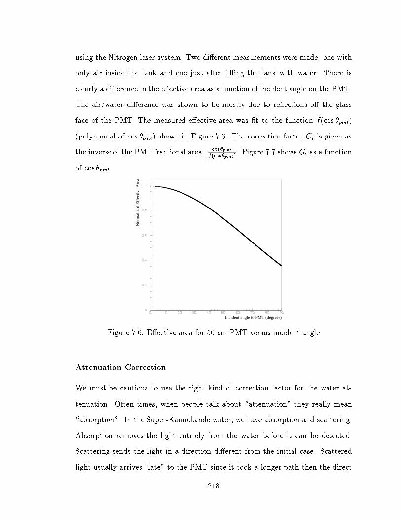
using the Nitrogen laser system. Two di�erent measurements were made: one with
only air inside the tank and one just after �lling the tank with water. There is
clearly a di�erence in the e�ective area as a function of incident angle on the PMT.
The air/water di�erence was shown to be mostly due to re ections o� the glass
face of the PMT. The measured e�ective area was �t to the function f(cos �pmt)
(polynomial of cos �pmt) shown in Figure 7.6. The correction factor Gi is given as
the inverse of the PMT fractional area: cos �pmt
f(cos�pmt). Figure 7.7 shows Gi as a function
of cos �pmt.
Incident angle to PMT (degrees)
Nor
mal
ized
Effe
ctiv
e A
rea
Figure 7.6: E�ective area for 50 cm PMT versus incident angle
Attenuation Correction
We must be cautious to use the right kind of correction factor for the water at-
tenuation. Often times, when people talk about \attenuation" they really mean
\absorption". In the Super-Kamiokande water, we have absorption and scattering.
Absorption removes the light entirely from the water before it can be detected.
Scattering sends the light in a direction di�erent from the initial case. Scattered
light usually arrives \late" to the PMT since it took a longer path then the direct
218

Incident angle to PMT (degrees)
Geo
met
rical
Cor
rect
ion
Fac
tor
G
Figure 7.7: Geometrical correction factor for Ne�ective
way from the production point to the PMT. Often times `di�use attenuation" is
measured using cosmic-ray muons. For these through-going muons, the charge (af-
ter some geometrical corrections) in each PMT is plotted versus the photon travel
distance in the water. A `di�use attenuation length' of 78 m is extracted by �tting
an exponential to this distribution. This is not the same measure of attenuation as
is needed for Ne�ective. The total PMT charge in a muon event will include some
light that was scattered and arrived late. If the PMT gets hit by `direct' light, the
QAC gate will already be open and the scattered light will contribute to the total
charge for that hit. This will not happen for low energy events. There are so few
tubes hit in a low energy event, that the chances of light scattering to a PMT which
was already hit is very unlikely. That means scattered light is detected by a `new'
PMT. Scattered light can not arrive very late and still have the hit count as an
\in time" tube. Ai needs to correct for absorption and the small angle scattering
which still arrives \in time".
To ensure the applicability in Ne�ective, the attenuation correction factor Ai
219

should be extracted from the calibration data. We chose to use data from the
nickel gamma-ray calibration source to �nd Ai. We looked at the probability of
getting an \in time signal" PMT hit as a function of distance (P (r)) the light must
travel to the PMT. To get this distribution correctly, two di�erent background
subtractions must be done. We made several distributions which are used for
background subtraction to get the �nal `probability versus distance'. To remove
any geometrical e�ects (see next section), we require the incident angle on the wall
to be nearly normal (cos �pmt > 0:9) for a tube to go into any histogram. Using
nickel source data at many di�erent locations, we made several versions of the \#
hits versus travel distance" distributions (listed below). \In time" (\out of time")
tubes have -10 < �ti < +20 ns (+300 < �ti < +330 ns).
� Dist. # 1 : 10 < �tfission < 110�s using \in time" tubes
(nickel events, signal PMT hits)
� Dist. # 2 : 10 < �tfission < 110�s using \out of time" tubes
(nickel events, noise PMT hits)
� Dist. # 3 : 400 < �tfission < 500�s using \in time" tubes
(background events, signal PMT hits)
� Dist. # 4 : 400 < �tfission < 500�s using \out of time" tubes
(background events, noise PMT hits)
� Dist. # 5 : \# PMTs versus travel distance" histogram using all tubes (this
is just the apparent geometry of the detector from the vertex; an entry is
made once for every ID PMT)
where �tfission is the time since the �ssion trigger (see Section 3.3.4). To remove
the histogram contribution from PMT dark noise, we take (Dist. # 1(3) - Dist.
220

# 2(4)) to yield distributions for `in time signal hits only'. As was discussed in
Section 3.3.4, the non-nickel events are removed by background subtraction. The
background is identi�ed as the events very late compared to the �ssion trigger while
the signal comes soon after the �ssion trigger. We need to account for the density
of PMTs not being uniform. The PMT density is contained in Dist. #5. The net
e�ect of all these steps is:
P (r) =[Dist: #1�Dist: #2]� [Dist: #3 �Dist: #4]
Dist: #5(7.5)
This probability function P (r) is the `raw' probability of getting a PMT hit as a
function of distance. The 1r2
drop o� in light intensity has not yet been removed
from P (r). The amount of attenuation (A) as a function of distance is equal to
P (r) � r2. The nickel data told us that A �ts well to the functional form:
A(r) = A1 exp�� r
L1�+A2 exp
�� r
L2�
(7.6)
where L1 and L2 are attenuation lengths and A1 and A2 are the weights of each
component. The attenuation correction would then be:
Ai =1
A(ri) (7.7)
where ri is the distance from the vertex to the ith PMT. We could not, however,
obtain reliable �t parameters from the data. Because of the low PMT density at
small distances, the error bars on A(r) were large. At longer distances where thestatistics are higher, the higher PMT density at the corners caused some problems
with the shape of A(r). Instead of �ddling around with excluding certain regions
from the �t to A(r), we decided to take a more straightforward approach.
We empirically determined the values of L1, L2, A1, and A2 by changing the
values and studying the uniformity of Ne�ective from the nickel source across the
221

�ducial volume. Starting values for the parameters came from our initial �t to the
nickel data. The parameters were varied until Ne�ective was most uniform across
most of the �ducial volume (a slight drop in Ne�ective at the edge was allowed since
the charge correction would bring the value back up). Before this optimization, it
was decided that no attenuation correction should be applied for distances shorter
than 5 meters. We then need to ensure that the correction function is normalized
at a distance of 5 meters. The best �t function is (shown in Figure 7.8):
ri > 5 m Ai = A(ri) =exp( r
200 m)+0:1exp(r
22 m)exp( 5 m
200 m)+0:1exp( 5 m
22 m)
ri � 5 m Ai = 1:
(7.8)
Distance (m)
Atte
nuat
ion
Cor
rect
ions
Figure 7.8: Attenuation correction factor for Ne�ective
Charge Correction
The attenuation and geometry corrections yield an Ne�ective which is fairly uniform
across the detector's �ducial volume. However, there is still a drop in Ne�ective over
the last few meters near the �ducial edge. We know that the probability of getting
a multi-pe hit increases as the production point of the �Cerenkov light approaches
222

the wall. This e�ect can be included in Ne�ective by a larger weighting factor for the
high charge tubes.
To determine what this weighting factor should be, the PMT charge distribution
for nickel events was studied. We plotted the di�erence between the distribution of
qi for nickel events at the center and at the �ducial volume edge. There was a clear
di�erence in the number of PMT hits with qi > 1:7 pe. These tubes are the ones
with real 2 pe signals (or occasionally larger). Clearly these hits need to count more
than the ones with smaller charge, but we do not want to overcompensate. We also
don't want to overweight a tube that may have extraordinarily high charge. Of the
methods tested, the simplest weighting scheme seemed to work the best:
if qi � 2:0 pe Ci = 1:0
if qi > 2:0 pe Ci = 2:0(7.9)
7.4.3 Performance of Ne�ective on Nickel Data
The entire point of making the corrections which make up Ne�ective is to remove
the detector e�ects. We need to verify that the Ne�ective energy scale is indeed
uniform across the �ducial volume. We do this using the nickel gamma-ray source.
Table 7.13 shows the �t mean and Gaussian width from the Ne�ective distribution
from the nickel data as a function of source position. The Ne�ective distributions
from the nickel source are background subtracted. Also given is the same quanti-
ties extracted from the MC simulation of the nickel source. The mean value of the
data Ne�ective is constant across the �ducial volume to <2% (the two points with a
* in Table 7.13 are outside the �ducial volume). Therefore, Ne�ective meets the most
important requirement for the energy scale parameter. The Ne�ective distribution
from the nickel data is about 5% wider than that from nickel Monte Carlo. This
may be due to the water absorption and scattering models or the nickel gamma-ray
223

spectrum in the MC not fully reproducing the data. The N50 distributions for data
and MC had di�erent widths which may support these reasons.
Ne�ective for Nickel Source
Source Position Mean Gaussian Width
Data MC Data MC
(cm) (hits) (hits) (hits) (hits)
(35, -70, 0) 41.29 42.18 12.59 10.91
(35, -70, 1200) 41.87 41.48 11.98 10.87
(35, -70, 1600) 41.08 39.59 11.18 10.20
(35, -1200, -1200) 41.43 41.21 12.05 10.36
(35, -1200, 0) 41.15 41.53 12.45 10.83
(35, -1555, -1200) * 38.43 38.12 11.79 9.93
(35, -1555, 0) * 38.94 38.63 11.68 9.99
* denotes the source as outside the �ducial volume
Table 7.13: Means and widths of Ne�ective from nickel data and MC
As with the N50 distributions, the Ne�ective mean values do not precisely agree
between Monte Carlo and data. These two points together indicate that the input
parameters are not yet entirely correct. They are close however. Probably the
inputs that need to be \tweaked" a bit still are the water attenuation and scattering
and the PMT angular acceptance.
224

7.4.4 Energy from Ne�ective
We have shown that the Ne�ective distributions from the Monte Carlo simulated
nickel source and from the real nickel calibration source match fairly well. Ideally,
we would use the LINAC data to tell us how to get from Ne�ective to electron total
energy in MeV. One problem with this approach is that the LINAC data is taken
only at one position in the detector and with only one direction. Even though our
energy scale (Ne�ective) is fairly uniform over the detector volume, we do not want
to introduce a potential bias to the energy scale.
Also, there are still questions about the proper interpretation of the LINAC
data which impact the energy calibration. When the �rst LINAC data was taken
in December 1996, it was discovered that the end cap obstructed the paths of a
fairly large percentage of the �Cerenkov photons (on the order of 10% at low ener-
gies). Due to the geometry and the path length di�erence between 15 MeV and
5 MeV electrons, the fraction of light which is shadowed by the beam pipe is energy
dependent. A new ange was designed to reduce the shadowing and was installed
for the January LINAC run. The shadowing is much smaller than before, but still
non-negligible.
For these reasons, we have chosen to perform the \absolute energy calibration"
using the events simulated by the tuned Monte Carlo program. We will use the
LINAC data as a sanity check on both the energy calibration and the systematic
error assigned to the energy scale. We generated monoenergetic electron events
with isotropic directions and vertices uniformly distributed throughout the �ducial
volume. For these event samples, the Super-Low Energy trigger was implemented
in the MC. This way little bias is introduced by the trigger e�ciency at low energies.
225

The Ne�ective distributions for each generated electron energy are �t to a Gaussian.
The mean values from the �t are graphed versus electron energy in Figure 7.9.
We �t the data points in Figure 7.9 to both a straight line and to a quadratic.
The �2 per degree of freedom for the quadratic �t was approximately one. The
linear �t yielded a �2 per degree of freedom almost an order of magnitude larger.
We use the best �t quadratic relationship between Ne�ective and the total electron
energy for each �ducial volume used in this analysis:
22.5 kton �2� = 1:23 Ne�ective = �7:7909 + 6:6665 � Etotal � 0:0228 � E2total
11.7 kton �2� = 0:80 Ne�ective = �7:4556 + 6:6514 � Etotal � 0:01678 � E2total
(7.10)
The non-linearity is believed to be caused by the incomplete accounting of multi-pe
PMT signals in Ne�ective. We do have a heavier charge weighting for PMTs that
measure larger signals, but it is very simple. A PMT with 3 pe counts the same
as a PMT with only 2 pe This insu�cient charge weighting causes Ne�ective to fall
o� at larger energies. So the best �t is non-linear. This conclusion is supported
by the best �t curve for the smaller �ducial volume (11.7 kton). When the higher
energy events are con�ned near the center of the detector, fewer PMT hits will have
multi-pe signals. The quadratic term will then be smaller for the 11.7 kton FV than
for the 22.5 kton FV. This has indeed been observed. To estimate the variation
in the conversion from Ne�ective to total energy due to Ne�ective not being uniform
across the volume, we also plot in Figure 7.9 some data points corresponding to
MC events generated only at the center of the detector.
226
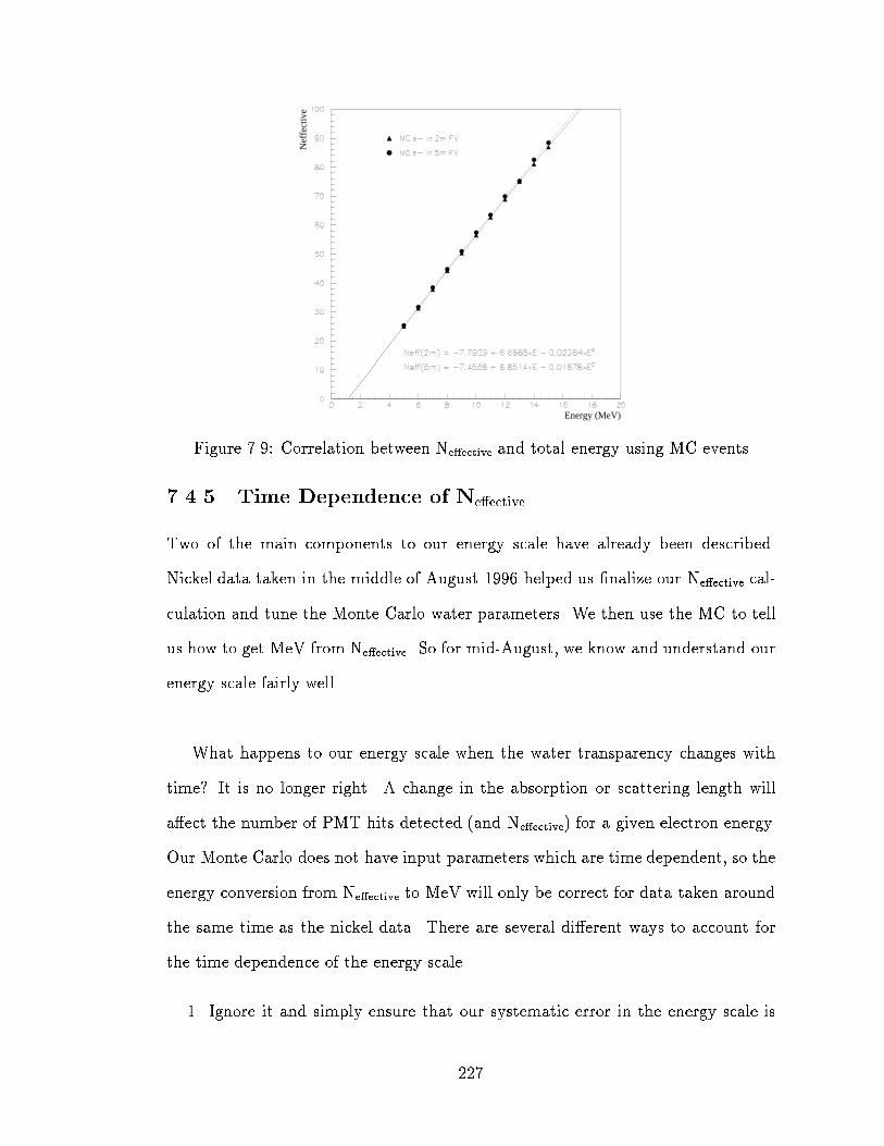
Energy (MeV)
Nef
fect
ive
Figure 7.9: Correlation between Ne�ective and total energy using MC events
7.4.5 Time Dependence of Ne�ective
Two of the main components to our energy scale have already been described.
Nickel data taken in the middle of August 1996 helped us �nalize our Ne�ective cal-
culation and tune the Monte Carlo water parameters. We then use the MC to tell
us how to get MeV from Ne�ective. So for mid-August, we know and understand our
energy scale fairly well.
What happens to our energy scale when the water transparency changes with
time? It is no longer right. A change in the absorption or scattering length will
a�ect the number of PMT hits detected (and Ne�ective) for a given electron energy.
Our Monte Carlo does not have input parameters which are time dependent, so the
energy conversion from Ne�ective to MeV will only be correct for data taken around
the same time as the nickel data. There are several di�erent ways to account for
the time dependence of the energy scale.
1. Ignore it and simply ensure that our systematic error in the energy scale is
227

large enough to account for this e�ect
2. Re-tune the MC parameters to nickel data taken each month (for example)
and get a time dependent conversion from Ne�ective to MeV
3. Scale Ne�ective by a time dependent multiplicative factor which equals one in
mid-August
4. Recompute Ne�ective with a time dependent attenuation correction (Ai(t))
This last method is the correct thing to do. For this analysis, the necessary time
to develop an appropriate Ai(t) was not available. We resort to applying method
#3: a time dependent scaling of Ne�ective.
We need some way to determine the overall scaling factor for Ne�ective. One
option might be to use the nickel data taken at a particular location. We could
compute the mean Ne�ective for nickel data taken at various times with the source
positioned at the center (for example). If we normalized Ne�ective to the mid-August
value, we could perform a �t to the resultant points. The best �t function could
then be used as the multiplicative scaling factor. Two problems crop up with this
idea. One is that we have periods of time where no nickel data was taken. The sec-
ond is that the correction derived from data taken at a single place in the detector
would, strictly speaking, be an appropriate correction for events with vertices near
that place. Since we are making an average correction to the events in the �rst
place (because we did not go with option #4 above), we really need to derive the
scaling factor in a way that averages over all positions in the detector.
Clearly we want to use the data somehow to derive the Ne�ective scale factor.
We need a source of events in the solar neutrino energy range from which we have
228

data at various times throughout the entire time period of the solar neutrino data
set. There is always spallation occurring in the detector. The spallation products
are a �ne source to use for monitoring Ne�ective. It might be preferable to select a
particular product isotope and monitor the Ne�ective changes in that single � decay.
That is not easy to do in practice and is not really necessary. We just need a well
de�ned sample of events to use for this study.
We chose to use events occurring within 100 ms and 1.5 m of a previous muon.
The events are separated into monthly samples and the central region of the Ne�ective
distributions are �t to Gaussians. Figure 7.10 shows one of the distributions with
the best �t. The �t mean Ne�ective values are plotted as a function of time in
Figure 7.11. The best �t polynomial function is shown. Note that hNe�ectivei fromthe peak to the valley changes on the order of 7%. If hNe�ectivei is normalized to
the middle of August (when the nickel data was taken which the Monte Carlo was
tuned with) and inverted, the multiplicative scaling factor is obtained (shown in
Figure 7.12). On an event by event basis, we take the Ne�ective computed for the
event, multiply by the correction factor appropriate for the date on which the event
occurred, and then convert to MeV (energy). At most, we scale Ne�ective up by 3%
or down by 1.5%.
7.4.6 LINAC results
The LINAC data does not always consist of perfect, single electron events. The data
must be \cleaned" up in order to do a reliable energy calibration. The problem is
that the LINAC trigger can be generated when there 0, 1, 2, or more electrons in the
same bunch. If no electron is present, the trigger was caused by random noise in the
trigger counter (PMT and thin plastic scintillator). Noise is not a problem when
229

Figure 7.10: Ne�ective from selected spallation events in August
Figure 7.11: Time dependence of �t Ne�ective from selected spallation events
230
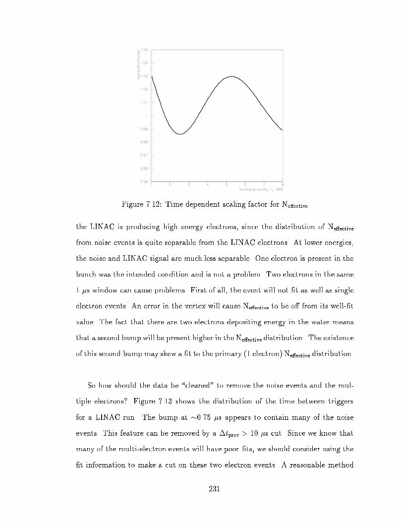
Figure 7.12: Time dependent scaling factor for Ne�ective
the LINAC is producing high energy electrons, since the distribution of Ne�ective
from noise events is quite separable from the LINAC electrons. At lower energies,
the noise and LINAC signal are much less separable. One electron is present in the
bunch was the intended condition and is not a problem. Two electrons in the same
1 �s window can cause problems. First of all, the event will not �t as well as single
electron events. An error in the vertex will cause Ne�ective to be o� from its well-�t
value. The fact that there are two electrons depositing energy in the water means
that a second bump will be present higher in the Ne�ective distribution. The existence
of this second bump may skew a �t to the primary (1 electron) Ne�ective distribution.
So how should the data be \cleaned" to remove the noise events and the mul-
tiple electrons? Figure 7.13 shows the distribution of the time between triggers
for a LINAC run. The bump at �0.75 �s appears to contain many of the noise
events. This feature can be removed by a �tprev > 10 �s cut. Since we know that
many of the multi-electron events will have poor �ts, we should consider using the
�t information to make a cut on these two electron events. A reasonable method
231

of accepting only good �ts is to make a cut on the value of T0 from Combo�t.
Figure 7.14 gives the T0 distribution for all the events during a LINAC run. The
acceptable range of T0's is indicated on the plot (750 - 900 ns).
Time since previous event (ns)
#/bi
n
Time since previous event (ns)
#/bi
n
Figure 7.13: Time since the previous trigger from LINAC data
We apply these two cuts (�tprev and T0) to the LINAC data, compute Ne�ective
for each event, and �t the resultant distribution to a Gaussian. The mean and
width of Ne�ective as a function of computed electron energy is given in Table 7.14.
We compare the LINAC results to the Monte Carlo values. Since this LINAC data
was taken in January 1997 and the MC was tuned to August 1996 nickel data, we
need to apply the scaling factor discussed in Section 7.4.5. Both the scaled and
unscaled results are given in the table. Also displayed are the mean and width
of Ne�ective for Monte Carlo events simulated at the LINAC beam energies. The
MC electrons were given vertices at the same location as the end of the LINAC
beam pipe. The electron directions pointed straight down. The end cap geometry
was not simulated so there is no shadowing of the �Cerenkov light for the MC events.
232

T0 from Combofit (ns)
#/bi
n
Figure 7.14: T0 from Combo�t applied to LINAC data
Ne�ective for LINAC
Beam Energy Mean Gaussian Width
Data Scaled Data MC Data Scaled Data MC
(MeV) (hits) (hits) (hits) (hits) (hits) (hits)
5.866 31.07 30.72 30.02 9.02 8.87 7.80
6.782 38.70 38.27 36.10 10.37 10.22 8.32
8.637 51.85 51.26 48.31 11.74 11.60 9.38
15.966 99.91 98.80 93.84 14.77 14.68 12.63
Table 7.14: Ne�ective results from LINAC data and MC
233

From Table 7.14, we can see that the scaled LINAC data and the Monte Carlo
do not perfectly agree even after the time dependent correction to Ne�ective. The de-
viation in the mean Ne�ective from scaled data to MC is �5%. This di�erence couldbe caused by several di�erent things. The �rst is the cleaning technique applied
to the LINAC data. By changing how the \single electron" peak is selected out
prior to �tting, we can change the mean Ne�ective by up to a few percent. Also, the
LINAC data occurs at the end of the time period for which our Ne�ective correction
is valid. It is quite possible that when the month of February is included in the �t
of Ne�ective versus date that the actual values of the correction factor on the date of
the LINAC data will change. Given the uncertainty in the validity of this LINAC
to MC comparison, we do not take this 5% di�erence into account when computing
our systematic errors.
The fractional energy resolution measured using the LINAC data is fairly well
reproduced by the MC. Figure 7.15 shows the energy resolution measured using the
LINAC and MC events. The best �t to the LINAC data yields a parameterization
for the energy resolution of the following form:
�E =17:5%q
E10 MeV
=55:4%p
E(7.11)
7.5 Radon
Radon gas creates background events in underground solar neutrino detectors[72].
Radon is a noble gas (222Rn) which easily di�uses through materials. Radon is a
problem because it is radioactive with a half life of 3.8 days. The decay of radon
leads to a long chain of unstable elements whose decays result in many low energy
� and emissions. The member of the chain with the highest energy � decay is
234

Energy (MeV)
Ene
rgy
Res
olut
ion
(%)
Figure 7.15: Reconstructed energy resolution using MC and LINAC data
214Bi:
214Bi �!214 Po + e� + �e (7.12)
which has an end point � energy of 3.26 MeV. The rest of the decays in the chain
have even less energy than this reaction. Although this end point energy (the
largest energy which the ejected electron may carry) is technically below Super-
Kamiokande's trigger threshold, uctuations in the number of detected �Cerenkov
photons will sometimes allow these events to trigger the detector. If radon gas is
very plentiful, Super-Kamiokande will trigger a lot just on the radon. Using the
MC with a simplistic generator for the 214Bi decay, we estimate the Low Energy
trigger e�ciency to be on the order of 0.2% for 214Bi � decays.
As construction of the detector took place, the radon content of each material
was measured [73]. From our in situ measurements, the radon content in the detec-
tor is � 2:0� 10�2 Bq/m3 or � 5:4� 10�4 pCi/l (compared to the Kamiokande-III
concentration of � 0:1 Bq/m3 or 2:7 � 10�3 pCi/l). Given the trigger e�ciency,
this radon concentration does not even account for half of the Low Energy triggers.
235

Even though the radon level does not explain the trigger rate, we still get many
background events produced by the radon decay daughters.
As far as we know, radon events are not preferentially clustered in particular
areas of the detector volume. They are real events in the sense that an elec-
tron or gamma-ray produced �Cerenkov light which assisted in generating a Super-
Kamiokande trigger. With our current knowledge there is no real way to cut radon
events out of the data sample except to reduce the radon content in the real de-
tector. Radon can enter Super-Kamiokande via the water system or di�using in
from the air above the tank. The radon working group is developing methods to
reduce the radon contamination in the detector and to monitor the radon level in
the Super-Kamiokande water and air.
7.6 \Flashers"
As we processed the data and monitored the data quality, we discovered sporadic
excesses in the number of \junk" events ending up in our data sample. These \junk"
events were found by looking at distributions of the goodness of �t computed by
Hayai and Combo�t. We devised a cut on the goodness of the vertex �t to remove a
large fraction of these new \junk" events. Figure 7.16 shows the normal distribution
of the goodness of �t from Hayai and the distribution containing these junk events.
After veri�cation using the Monte Carlo, we make a cut at 0.5 to keep the good
events. We scanned the events failing this cut to try and identify the root source
of the triggers. We repeatedly observed the same PMT hit pattern. This is usually
indicative of having a \ asher" inside the detector. A \ asher" is a PMT which
intermittently emits light (usually generated by arcing inside the PMT). A \ asher"
is almost always near the end of its life. It is possible to devise methods tag
236

potential \ asher" events on an event by event basis, but nothing of that sort has
been implemented in this thesis. We rely on the goodness of the Hayai �t to reduce
the number of asher events in our �nal solar neutrino sample.
Goodness of Hayai fit
no. o
f eve
nts/
bin
Figure 7.16: \Flasher" cut using the goodness of Hayai �t distributions
237

Chapter 8
Results
8.1 Data Set
On April 1, 1996 Super-Kamiokande became fully operational and started collect-
ing data full time. As with any new experiment, it took a while to work out the
little problems and understand what was going on with the detector as a whole.
The water needed time to be further cleaned by the water puri�cation system so
the water transparency would stabilize. This �rst data is therefore excluded from
this solar neutrino analysis.
The �nal data set used in this analysis contains the data from May 24, 1996
through February 10, 1997. This corresponds to Runs 1679 through 3523. There
are approximately 10 days of data from the beginning of August which we did not
process because of a `TQ real' problem which set the PMT times to zero for all
the high charge PMTs. Approximately 251 calender days of data are contained
in this data set. The vertex cut of Dwall � 2 meters implies a �ducial volume of
22.485 kton 1 (out of the 32.481 kton inner detector volume). The Cubist exposure
1In this thesis, a ton refers to a metric ton or a cubic meter.
238

and e�ective live time (for the 22.801 kton volume considered active by Cubist) are
given in Table 8.1. The full data set will be broken down into data collected at
night and during the day.
Data Set Cubist Exposure E�ective Live Time
All 3376.3 kton-days 148.2 days
Day 1600.0 kton-days 70.2 days
Night 1776.3 kton-days 77.9 days
Table 8.1: Exposure for �nal data sample
These exposures make sense, given all the places where live time can be lost.
First of all, the detector is only live 85% of the time each week. The remainder
of the time is spent on calibration, hardware tests and replacement, water trans-
parency measurements, and ` asher' �nding expeditions. The good run criteria
removes almost 20% of the subruns leaving the analysis live about 85% of the time.
Spallation and other Cubist cuts reduce the live time by another 15%. Putting all
these losses together yields an expected live time of about 154 days. The Cubist
exposure is then quite reasonable:
154 days = 251 days� 0:85 � 0:85 � 0:85:
8.2 \Interactive" Cuts
After le ntuple processing, more cuts are applied to the data via NTUPLE cuts.
These cuts are done interactively using PAW so there is no output �le created. The
cuts can be easily modi�ed without the hassle of re-processing the entire data set.
If desired, a new NTUPLE can be written out with only the events after certain
239

cuts. The spallation cuts are applied through the NTUPLE. If Cubist returned a
non-zero value, the event has not passed all the cuts. We also make the \ asher"
cut (GOFh > 0:5) described in Section 7.6. The last cut is on the energy of the
event. We want to use the events in the energy range where we are con�dent about
knowing the e�ciencies and where the e�ciency is very high and at with energy.
If you use the range where the e�ciency is falling, it is important to know the shape
of the falling edge well. For this reason, we only consider events above an energy
threshold of 6.5 MeV.
8.3 Characteristics of Final Event Sample
We started out with raw data which had lots of problems and events which we
wanted to remove from the data set. We developed �ltering software and a variety
of cuts designed to clean up the data and leave us with only viable solar neutrino
candidate events, our �nal data sample. Figure 8.1 shows the �t coordinate distri-
butions from the �nal sample events after the GOF and spallation cuts and with
Ereconstruct > 7 MeV. Note that the number of events per bin in the R2 plot rises at
the edge of the �ducial volume. There is also a peak in the Z coordinate distribution
near the bottom of the tank. The �t direction cosines for the same events are given
in Figure 8.2. Note that the x and y direction cosine (dx and dy) distributions
are pretty much at, while the z direction cosine (dz) distribution has a distinctly
non at shape. In addition, the Z and dz distributions are both asymmetric. The
�nal sample has many events whose �t vertex is near the edge of the �ducial volume
or outside it and whose direction points towards the center of the detector. These
events are typically referred to as \gammas from the rock" and form an anisotropic
background for the solar neutrino signal. We know frommeasurementsmade by the
Kamiokande collaboration [74] that there are many gamma-rays emanating from
240

the rock face. Some of these gammas will penetrate through to the inner detector
volume and generate a trigger. These \ s from the rock" will �t near the wall
with directions pointing in. Also, radioactive impurities in the glass envelope of the
50 cm PMTs may generate gamma rays which trigger the detector. These events
will also have �t vertices close to the inner detector walls (where the PMTs are
located). The energy distributions for all events above 7.0 MeV passing the GOF
cut and the spallation cut are given in Figure 8.3.
Next we want to know if we can see a correlation between our events and the
Sun. Figure 8.4 displays example of our standard `solar peak' distributions after
the spallation cuts. The GOF cut and a 7 MeV energy threshold were applied. The
quantity histogrammed is:
cos �sun = �~devent � ~dsun (8.1)
where ~devent is the �t direction of the event and ~dsun is the direction vector from
the center of the Super-Kamiokande tank to the Sun (in the Super-Kamiokande
coordinate system). We expect a strong peak at cos �sun = 1 for events initiated
by neutrinos coming from the Sun. Indeed, we see a clear peak from the Sun.
Figures 8.5 and 8.6 show the same cos �sun distributions after breaking up the data
into day and night samples. Note that the backgrounds do not look at.
8.4 Signal Extraction Method
In order to compute a solar neutrino ux, we need some way to extract the number
of solar neutrino interactions in our �nal data sample. We tried several di�erent
methods and settled on a two step method of �tting the background level and then
the signal above the background. We took the shape of the background to be a
241

X C
oordinate (cm)
# events per 10 cm bin
Y C
oordinate (cm)
# events per 10 cm bin
T0 (ns)
# events per 10 cm bin
Z C
oordinate (cm)
# events per 10 cm bin
R2(cm
2)
# events per 1 m2 bin
Figu
re8.1:
Vertex
coordinate
distrib
ution
sfrom
�nalsam
ple
242

X direction cosine
# events per 0.01 bin
Y direction cosine
# events per 0.01 bin
Z direction cosine
# events per 0.01 bin
Figu
re8.2:
Direction
cosinedistrib
ution
sfrom
�nal
sample
243

Total Energy (MeV)
# ev
ents
per
0.1
MeV
Total Energy (MeV)
# ev
ents
per
0.1
MeV
Figure 8.3: Energy distribution from �nal sample (linear and semi-log plots)
cosθsun for ALL data
Eve
nts
per
0.02
5 bi
n
Figure 8.4: Correlation between the Sun and �nal sample event directions
244

cosθsun for DAY data
Eve
nts
per
0.02
5 bi
n
Figure 8.5: Solar peak for the day data with Ereconstruct > 7 MeV
cosθsun for NIGHT data
Eve
nts
per
0.02
5 bi
n
Figure 8.6: Solar peak for the night data with Erecontruct > 7 MeV
245

straight line with non-zero slope. A non- at background was implemented after
looking at the day and night cos �sun distributions. For consistency, we let the slope
oat for the ALL data, even though the �t to a at background gives a similar �2.
The background is intrinsically not at, as we have an excess of events near the
bottom pointing up. The background level is determined by a simple �2 �t to a
linear background using the data with �1 � cos �sun < +0:5. We then extrapolate
this best �t line (over the full range of cos �sun) to predict the background under-
neath the solar neutrino peak.
Once the number of background events in each bin is found, the excess events
can be �t to the shape of cos �sun predicted by the Monte Carlo for the current
energy threshold. Figure 8.7 shows the various cos �sun MC shapes (normalized to
unit area) used for the �ts to the data. A �2 minimization is used to �nd the
total number of signal events above background. The statistical error in the total
number of signal events is obtained by varying �2 by one unit. Figure 8.8 shows
the minimum and the variations in �2 from the �t to the full �nal sample with
Ethreshold > 7 MeV.
8.5 Measured Solar Neutrino Event Rate
We use the described method of extracting the number of solar neutrino events for
each subset of the data which is of interest. Speci�cally, we apply several di�erent
energy thresholds to the �nal sample. We also break up the data into day-only and
night-only event samples to look for a day/night di�erence. Day is de�ned to be
when the Sun is above the horizon ((dsun)z � 0) and night occurs when the Sun
is below the horizon ((dsun)z < 0). As a consistency check, two di�erent �ducial
volumes are used - the 22.5 kton volume previously mentioned and a 11.7 kton
246

cosθMC sun
Nor
mal
ized
Pro
babi
litie
s
Figure 8.7: cos �sun shapes predicted from the Monte Carlo
Extracted Number of Signal Events
χ2 Val
ue
Figure 8.8: �2 minimum for �t to background + solar neutrino signal
247

volume (created by making a Dwall � 5 meter cut). For each of these subsets of
data, the �t background and signal levels are given in Table 8.2 or Table 8.3.
22.5 kton �ducial volume
Ethreshold BG level BG slope Signal Excess
(MeV) (events) (ev./bin, 80 bins) (events) (events/day)
All data, 148.07 day sample
6.5 MeV 1382.0 14.6 2796 � 128.0 18.884 � 0.864
7.0 MeV 1027.5 12.7 2436 � 111.0 16.452 � 0.750
8.0 MeV 621.9 6.8 1757 � 86.0 11.866 � 0.518
10.0 MeV 171.2 4.2 737 � 47.0 4.978 � 0.317
Day data, 70.17 day sample
6.5 MeV 646.9 -22.4 1330 � 86.0 18.155 � 1.226
7.0 MeV 480.0 -14.9 1177 � 75.0 16.774 � 1.069
8.0 MeV 289.2 -18.9 903 � 57.5 12.869 � 0.819
10.0 MeV 79.1 -7.0 364 � 31.0 5.188 � 0.442
Night data, 77.90 day sample
6.5 MeV 734.2 37.7 1462 � 94.5 18.768 � 1.213
7.0 MeV 546.6 27.9 1257 � 82.0 16.137 � 1.053
8.0 MeV 332.0 25.7 848 � 63.5 10.886 � 0.815
10.0 MeV 91.3 11.0 367 � 35.0 4.711 � 0.449
Table 8.2: 22.5 kton measured signal and background rates
248

11.7 kton �ducial volume
Ethreshold BG level BG slope Signal Excess
(MeV) (events) (ev/bin, 80 bins) (events) (events/day)
All data, 148.07 day sample
6.5 MeV 598.1 4.3 1466 � 85.5 9.901 � 0.577
7.0 MeV 476.1 4.7 1316 � 77.0 8.888 � 0.520
8.0 MeV 293.1 1.3 893 � 59.5 6.031 � 0.402
10.0 MeV 78.5 0.7 390 � 32.0 2.634 � 0.216
Day data, 70.17 day sample
6.5 MeV 278.9 -9.4 683 � 57.5 9.734 � 0.819
7.0 MeV 221.5 -7.3 604 � 51.0 8.608 � 0.727
8.0 MeV 136.2 -9.3 415 � 39.0 5.914 � 0.556
10.0 MeV 35.4 -5.1 178 � 20.5 2.537 � 0.292
Night data, 77.90 day sample
6.5 MeV 318.5 14.7 776 � 63.5 9.962 � 0.815
7.0 MeV 253.6 13.0 704 � 57.0 9.038 � 0.732
8.0 MeV 156.0 11.2 474 � 44.5 6.085 � 0.571
10.0 MeV 42.0 5.6 211 � 24.0 2.709 � 0.308
Table 8.3: 11.7 kton measured signal and background rates
249

8.6 E�ciency
In order to compare the measured rate of solar neutrino events to the SSM predicted
rate, we need to know the e�ciency of detecting solar neutrino events. The most
logical way to �gure out this e�ciency is to model precisely what happens to the
neutrino interactions in the detector. Given this philosophy, we simulate many
(200,000) solar neutrino interactions in the Super-Kamiokande detector. To do this,
we select an energy from the predicted spectrum (Figure 4.1) for each neutrino. An
interaction point in the 32.5 kton inner volume is selected and the �nal kinetic
energy of the scattered electron is chosen from the shape of the energy dependent
scattering cross section. The electron is tracked through the water and the detector
trigger is modeled. The majority of the solar neutrino induced events do not trigger
the detector at all. Once the triggers are generated, the simulated events are sent
through the software �lters (lef1 and lef2). The \interactive" cuts are applied
also, except for the spallation cut. The e�ciency is calculated:
�total =# remaining events vs. generated E
# events generated with E in full 32.5 ktons (before trigger simulation)
(8.2)
Figure 8.9 shows this overall e�ciency as a function of generated electron energy
for several di�erent applied energy thresholds. Note that the maximum e�ciency
attained is �70%. This is because the e�ect of the �ducial volume cut is included
in our de�nition of e�ciency. The ratio of �ducial volume (22.485 kton) to the full
volume (32.481 kton) is about 70%.
8.7 SSM Expectation
To calculate the number of neutrino events expected per day from the Standard
Solar Model, we need the overall e�ciency of detecting and measuring a neutrino
250

Generated Energy (MeV)
Tot
al E
ffici
ency
(tr
igge
r +
sof
twar
e)
Figure 8.9: Total e�ciency versus generated energy
event, the neutrino-electron scattering cross section, the energy spectrum of the
incident neutrinos, and the total calculated ux of solar neutrinos. All of this in-
formation has been discussed already (Sections 4.1.1 and 8.6), it just needs to be
assembled together for the overall rate calculation.
The total rate of solar neutrino interactions in a perfect detector (Rperfect) is:
Rperfect =Z Emax
0Fssm(E�)
Z Tmax
0Ntarget
d�(E�; Te)
dTedTe dE� (8.3)
where E� is the neutrino energy, Fssm is the SSM calculated neutrino ux at energy
E� , Ntarget is the number of electron targets in the full inner detector volume, d�dTe
is
the di�erential scattering cross section for an electron-neutrino pair, and Te is the
kinetic energy of the scattered electron. The ine�ciencies and energy resolution
of the detector must be included in order to compare this expected rate to a real
measurement. To do this:
R =Z Emax
0Fssm(E�)
Z Tmax
0Ntarget
d�(E�; Te)
dTe�total(Te) dTe dE� (8.4)
where �total is the total e�ciency for an electron with kinetic energy Te to end
251

up in the �nal sample (given in Section 8.6). We use the cross section for �e � e
scattering with the radiative corrections applied[75]. For ���e and ���e scattering,Equation 4.1 is utilized. The neutrino spectrum is taken from Bahcall [59]. The
predicted solar neutrino event rates using the BP92 ux [7] of 8B neutrinos (5:69�106 �
cm2s) and the BP95 ux [4] (6:62�106 �
cm2s) are given in Table 8.4. Two di�erent
sets of numbers are presented in the table. The �rst section shows the rate of
solar neutrino interactions in the Super-Kamiokande detector. The second section
includes the e�ects of energy our detector's energy resolution and reconstruction -
the applied threshold is on Ereconstruct.
Perfect detector for all energies
Thresh. Egenerated (MeV) Expected Event Rate in 22.5 kton (events/day)
BP92 BP95
0 317.6 369.5
Calculated Super-Kamiokande e�ciency
Thresh. Ereconstruct (MeV) Expected Event Rate in 22.5 kton (events/day)
BP92 BP95
6.5 MeV 42.81 49.81
7.0 MeV 35.93 41.80
8.0 MeV 23.48 27.31
10.0 MeV 8.27 9.03
Table 8.4: SSM predicted solar neutrino event rates
252
8.8 Systematic Errors
In addition to the statistical error assigned to the measured signal, we will have a
systematic error. Systematic uncertainties originate from a variety of places. Each
contribution which we consider is presented along with the estimated magnitude of
the ux uncertainty. A summary is given at the end of the section.
8.8.1 Fiducial Volume
By looking at the vertex resolution di�erence between data and Monte Carlo, we
can estimate the possible error in the total �ducial volume of the detector. Table 6.7
shows that di�erence to be about 4 cm (Monte Carlo is wider). The resultant error
in the �ducial volume is:
�VV
= 2�R2maxZmax�2�(Rmax�4cm)2(Zmax�4cm)
2�R2maxZmax
Rmax = 1490 cm and Zmax = 1610 cm��VV
�22:5kton
= 0:78 %
Rmax = 1190 cm and Zmax = 1310 cm��VV
�11:7kton
= 0:98 %
(8.5)
Since the total number of observed neutrino events is directly proportional to the
detector volume, the error on the neutrino ux is also:
11.7 kton volume: (�F )Volume = 0:98%:
22.5 kton volume: (�F )Volume = 0:78%:(8.6)
8.8.2 Energy Scale
Since an energy threshold is applied to the data, it is important to know the magni-
tude of any possible shift in the energy scale. A scale shift may cause an energy cut
which was thought of as E > 7:0 MeV to really be E > 6:85 MeV. The uncertainty
in the energy scale has of several di�erent sources. First of all, the input parameters
253

to the Monte Carlo simulation were tuned such that the data taken with the nickel
source on one particular day agrees with the simulation of the source. If the gamma-
ray production from the nickel source is not simulated accurately, the Monte Carlo
will not produce the appropriate amount of light for a given electron energy. To
estimate the accuracy of the nickel gamma-ray simulation, we compared the on-site
and o�-site nickel gamma-ray model. By using two di�erent nickel gamma-ray sim-
ulations in conjunction with a single detector Monte Carlo, we look at the variation
in the mean N50 caused by the di�erent gamma-ray generators. A 0:5% di�erence
was found between the two.
Table 7.13 shows the agreement between Ne�ective for the Monte Carlo of the
nickel source and the nickel data at various source positions. The maximal varia-
tion between the two is 3.1%, but that is not a fair estimate of the scale uncertainty.
To determine the rms deviation between MC and data, we calculate the weighted
mean deviation and the corresponding weighted rms. We weight by the uncer-
tainty in the Ne�ective di�erences. By varying the range over which the Gaussian �t
to Ne�ective distribution is done, we can calculate the mean value of Ne�ective (for the
nickel data) to only 2%. We assign this 2% uncertainty as the weight to each of
the points. The calculated rms deviation in Ne�ective between nickel data and nickel
MC is then 0.77%. Being more conservative, a systematic of 1% is quoted.
Lastly, we have the contribution due to the conversion from Ne�ective to total
energy. When we �t Ne�ective(E) (described in Section 7.4.4), we calculate errors on
the �t parameters. By propagation of errors, we can estimate the uncertainty in
the conversion as a function of energy. This uncertainty is approximately 8�10�3%
above 7 MeV. If three errors are summed together in quadrature, a total error on
254

the energy scale of 1.12% is found.
Uncertainty Cause
0.5% Gamma-ray simulation from nickel source
1.0% Agreement between nickel data and MC
8 � 10�3% Conversion from Ne�ective to total energy
1.12% TOTAL �E (added in quadrature)
Table 8.5: Contributions to energy scale uncertainty
The systematic error on the solar neutrino ux (F) is not equal to the energy
scale systematic. To estimate �F , we use our program which calculates the total
expected rate of solar neutrinos given the detector e�ciency. Purposely, we insert a
shift in the energy scale (both upward and downward shifts to check for symmetry)
and study how the predicted rate above a 7 MeV threshold changes with the energy
scale shift. We extract the ux uncertainty:
(�F)Energy Scale = 2:6� �EE(%) = 2:6 � 1:12%
(�F)Energy Scale = 2:91%:(8.7)
8.8.3 Time Dependence of Energy Scale
We need to evaluate the uncertainty in the ux due to the time dependent correc-
tion applied to Ne�ective. We do this by varying the functional form of the correction
as a function of date, using the modi�ed function to scale the Ne�ective values of the
data, and observing the corresponding change in the measured neutrino ux. We
acquire the reasonable range of functional forms by performing many di�erent �ts
to the spallation product Ne�ective distributions and to the time variation of the
hNe�ectivei. We �t Ne�ective to a single Gaussian and to a double Gaussian. We also
255

try binning the data monthly versus weekly.
We select as maximum and minimum limits the two functions which envelope
the correction function we actually used. By using these limits to correct the
Ne�ective and calculate the measured solar neutrino ux, we estimate an uncertainty
in the ux of:
(�F)Time Dependence = 2:0%: (8.8)
8.8.4 Energy Resolution
If our Monte Carlo does not reproduce the energy resolution of the real detector, our
prediction of the number of expected events above a particular threshold will be o�.
The energy resolution describes the spread in observed energies given a particular
generated (or real) energy. When a spectrum of energies is observed by a detector
with �nite energy resolution, the shape of the spectrum changes. If the Monte Carlo
has a di�erent energy resolution than the data, the measured spectrum shape will
be di�erent from the MC prediction. The ux above a particular threshold energy
will also di�er between the MC and the data. To estimate the change in the
ux due to the energy resolution, we determine the energy resolution curves (see
Figure 7.15) which bracket the LINAC data (approximately 56% � 5%) and assume
that these curves are characteristic of 2� errors in the resolution. We use these three
resolution curves to generate the shape of fake e�ciency functions for use in the
SSM predicted rate calculation. The variation in the predicted event rates above
7 MeV was �1:27% at the 2� level. The 1� error therefore corresponds to:
(�F)Energy Resolution = 0:64%: (8.9)
256
8.8.5 Signal Extraction
When we extract the number of solar neutrino excess events, we introduce several
places for potential errors. We �t the cos �sun distribution to the shape predicted by
the Monte Carlo. What if this shape is not representative of the real shape produced
by the data? To mimic this problem, we �t the data with a threshold of Ethreshold
applied using the Monte Carlo shapes corresponding to Ethreshold� 1 MeV. We can
then look at the di�erence in the measured ux from using a shape corresponding
to a 1 MeV shift in energy (to get the ux di�erence per MeV shift). To compute
the actual error, we scale the ux uncertainty per MeV shift by the systematic error
in the energy scale (1.12%). The net result is
(�F)Signal Shape = 0:25%; (8.10)
the ux uncertainty due to the incorrect cos �sun shape.
In addition to using the correct shape for the cos �sun distribution, the back-
ground level must also be correct. If the background level is mis�t or undergoes
large uctuations, the signal above background will be nearly impossible to �t re-
liably. To estimate the maximum magnitude of this potential error, we varied the
slope of the background level by �1� and observed how the extracted signal above
background changed. This is a conservative estimate of the maximum value for
the ux error due to the extrapolation of the background shape under the solar
peak. We have already assumed that the shape is consistent with a straight line.
By varying the slope by �1�, we are estimating the ux error higher than might be
considered reasonable. The deviation in the total number of signal events directly
tells us the error in the ux due to variations in the background level. The ux
uncertainties are given in Table 8.6 for several di�erent energy thresholds, data
samples, and �ducial volumes. These systematic uncertainties are due to the sta-
257

tistical accuracy of the points included in the background �t. They will decrease
with more statistics. They also will go down with an improved �t to the functional
form of the background.
Data Sample Fiducial Volume Ethreshold (�F)BG Fit
All 22.5 kton 6.5 MeV 3.25%
All 22.5 kton 7.0 MeV 3.16%
All 22.5 kton 8.0 MeV 3.30%
All 22.5 kton 10.0 MeV 3.87%
Day 22.5 kton 7.0 MeV 4.50%
Night 22.5 kton 7.0 MeV 4.50%
All 11.7 kton 7.0 MeV 4.03%
Day 11.7 kton 7.0 MeV 5.96%
Night 11.7 kton 7.0 MeV 5.47%
Table 8.6: Systematic ux uncertainty due to B.G. slope
8.8.6 Scattering Cross Section
The uncertainty is fairly small in the scattering cross section. The major contribut-
ing value is the uncertainty of 0.2% on sin2 �W . The ux error is conservatively taken
as:
(�F )Cross Section = 0:5%: (8.11)
8.8.7 Total Systematic Error
Each of the contributions to the systematic error on the solar neutrino ux has been
presented. These errors are typically combined together so that a single systematic
258

uncertainty is quoted for the ux. It is standard practice to add the component
errors in quadrature to yield a 1� total ux error. Although there are reasonable
arguments against such practice, we have no other way of interpreting the meaning
of the systematic error. For those who prefer to handle systematic errors in a
di�erent way, Table 8.7 provides a summary of all the contributions considered. A
shortened summary of the total error (adding in quadrature) is given in Table 8.8.
Contribution Energy Error Flux Systematic Error
Fiducial volume 0.78% - 0.98%
Nickel gamma-ray simulation 0.5%
MC/data agreement 1.0%
Ne�ective to MeV conversion 8.0 �10�3%Net Flux error 2.6% � Energy error
Time dependence 2.0%
Energy resolution 0.64%
Signal shape 0.25%
Background Fit 3.16% - 5.96%
�e + e cross section 0.5%
Table 8.7: Components of the total systematic error on solar neutrino ux
8.9 Measured Solar Neutrino Flux
Tables 8.9 and 8.10 display the solar neutrino ux results and the data/SSM ratios
for the two �ducial volumes analyzed. Note that the data/SSM ratios are not equal
to 1.0, indicating that we are observing fewer solar neutrinos than predicted. Also,
there is an energy dependence to the data/SSM ratio. This could be caused by a
259

Sample Volume Ethreshold Total Systematic Error
All 22.5 kton 6.5 MeV 4.94%
All 22.5 kton 7.0 MeV 4.88%
All 22.5 kton 8.0 MeV 4.97%
All 22.5 kton 10.0 MeV 5.37%
Day 22.5 kton 7.0 MeV 5.84%
Night 22.5 kton 7.0 MeV 5.84%
All 11.7 kton 7.0 MeV 5.51%
Day 11.7 kton 7.0 MeV 7.05%
Night 11.7 kton 7.0 MeV 6.64%
Table 8.8: Total systematic error on solar neutrino ux
systematic problem in the energy scale or by the neutrino spectrum being distorted
(as may happen in neutrino oscillations).
8.10 Measured Di�erential Energy Spectrum
To further explore the apparent energy dependence of the data/SSM ratio, we exam-
ine the di�erential energy spectrum of the data. Figure 8.10 shows the background
subtracted energy distribution of the �nal sample events above 6.5 MeV. The back-
ground subtraction was performed by assuming the region with cos �sun � 0:5 (S)
contains the solar neutrino signal plus background and �1 � cos �sun < 0:5 (B) has
background only. We assume the background level is at (see Section 8.4) with
cos �sun and simply subtract S� B3 energy bin by energy bin. The result is the data
distribution shown in Figure 8.10. The last bin contains all events above 14 MeV.
Statistical errors only are given on all three plotted distributions.
260

22.5 kton Fiducial Volume
Ethreshold
�FData
FSSM
�BP92
�FData
FSSM
�BP95
� (statistical error) � (systematic error)
All data
6.5 MeV 0.441 � 0.020 � 0.022 0.379 � 0.017 � 0.019
7.0 MeV 0.458 � 0.021 � 0.022 0.394 � 0.018 � 0.019
8.0 MeV 0.504 � 0.025 � 0.025 0.434 � 0.021 � 0.021
10.0 MeV 0.602 � 0.038 � 0.032 0.517 � 0.033 � 0.028
Day data
6.5 MeV 0.443 � 0.029 0.381 � 0.025
7.0 MeV 0.467 � 0.030 � 0.027 0.401 � 0.026 � 0.024
8.0 MeV 0.548 � 0.035 0.471 � 0.030
10.0 MeV 0.627 � 0.053 0.539 � 0.046
Night data
6.5 MeV 0.438 � 0.028 0.377 � 0.024
7.0 MeV 0.449 � 0.029 � 0.026 0.386 � 0.025 � 0.023
8.0 MeV 0.464 � 0.035 0.399 � 0.030
10.0 MeV 0.569 � 0.054 0.489 � 0.047
Table 8.9: Ratios of measured � uxes in 22.5 kton to the SSM predictions
261

11.7 kton Fiducial Volume
Ethreshold
�FData
FSSM
�BP92
�FData
FSSM
�BP95
� (statistical error) � (systematic error)
All data
6.5 MeV 0.446 � 0.026 0.384 � 0.022
7.0 MeV 0.477 � 0.028 � 0.026 0.410 � 0.024 � 0.023
8.0 MeV 0.500 � 0.033 0.426 � 0.021
10.0 MeV 0.614 � 0.050 0.528 � 0.043
Day data
6.5 MeV 0.439 � 0.037 0.377 � 0.032
7.0 MeV 0.462 � 0.039 � 0.033 0.397 � 0.034 � 0.028
8.0 MeV 0.486 � 0.046 0.418 � 0.039
10.0 MeV 0.591 � 0.068 0.508 � 0.059
Night data
6.5 MeV 0.449 � 0.037 0.386 � 0.039
7.0 MeV 0.485 � 0.039 � 0.032 0.417 � 0.034 � 0.028
8.0 MeV 0.500 � 0.033 0.426 � 0.028
10.0 MeV 0.632 � 0.072 0.543 � 0.047
Table 8.10: Ratios of measured � uxes in 11.7 kton to the SSM predictions
262

Reconstructed Electron Energy (MeV)
# ev
ents
/MeV
Figure 8.10: Di�erential energy spectra from the data and Monte Carlo prediction
Also given in Figure 8.10 is the SSM predicted spectrum. This distribution
comes from a Monte Carlo simulation of solar neutrinos with the predicted energy
distribution. The same background subtraction is applied to the MC as with the
data. The BP95 SSM distribution has been scaled to contain the predicted num-
ber of events our analysis would see over 148.2 live days. The third distribution
displayed in Figure 8.10 is the SSM spectrum scaled down by the observed integral
data/SSM ratio above a 7 MeV threshold (given in Table 8.9). Observe that the
scaled down SSM and the data do not appear to have the same shape.
Since the prediction of a distorted energy spectrum is one of the keys to new
neutrino physics, we want to further study the shape of the di�erential energy spec-
trum. We can plot the ratio of the observed spectrum to the predicted spectrum.
If the neutrino spectrum is not distorted, the data/SSM ratio will be constant
with energy. Figure 8.11 shows the data/SSM ratio as a function of reconstructed
electron energy. The last bin contains all events above 14 MeV. The error bars
263

indicate the statistical errors only. The systematic errors as a function of energy
have not yet been evaluated. Given these statistical errors, the probability that
this distribution �ts to a at line is <1% (�2 = 22.3, # DOF = 8).
Reconstructed Electron Energy (MeV)
Dat
a / B
P95
SS
M p
er 1
MeV
Ene
rgy
bin
Figure 8.11: Spectral shape of the data relative to the SSM prediction
The shape (slope) of the distribution in Figure 8.11 is greatly a�ected by energy
dependent systematic errors which have not yet been evaluated. We have evaluated
the e�ect of these energy errors on the integral ux above various thresholds. The
contribution to the systematic errors on the di�erential energy ux will be di�er-
ent. These systematics are currently under study and will not be presented here,
therefore Figure 8.11 should always be considered cautiously.
264

Chapter 9
Interpretation and Conclusions
9.1 Comparison with On-Site Group
As was mentioned previously, this dissertation describes only one of the solar neu-
trino analyses being performed by the Super-Kamiokande collaboration. A second
independent group based at the experimental site (On-Site group) also analyzes
the low energy data. The only thing the two groups have in common is that they
both have access to the same calibration data and both �lter and analyze the same
raw data. The philosophies driving the two groups are remarkably divergent. This
leads to very dissimilar �ltering algorithms and analysis techniques. The fact that
things are so di�erent has made performing direct comparisons between the two
groups quite challenging. On the other hand, the same result from two indepen-
dent analyses signi�cantly increases the con�dence in the robustness of the result.
The On-Site Low Energy group does most of their analysis o�-line and in semi-
real time. A farm of Sun workstations grabs the data out of memory (where the
`TQ real' process places the data) and starts �ltering. The �lter operates in several
stages and includes some `junk' cuts, a vertex �tter and �ducial volume cut, and
a single muon �tter. They apply good run criteria, implement spallation cuts, and
265
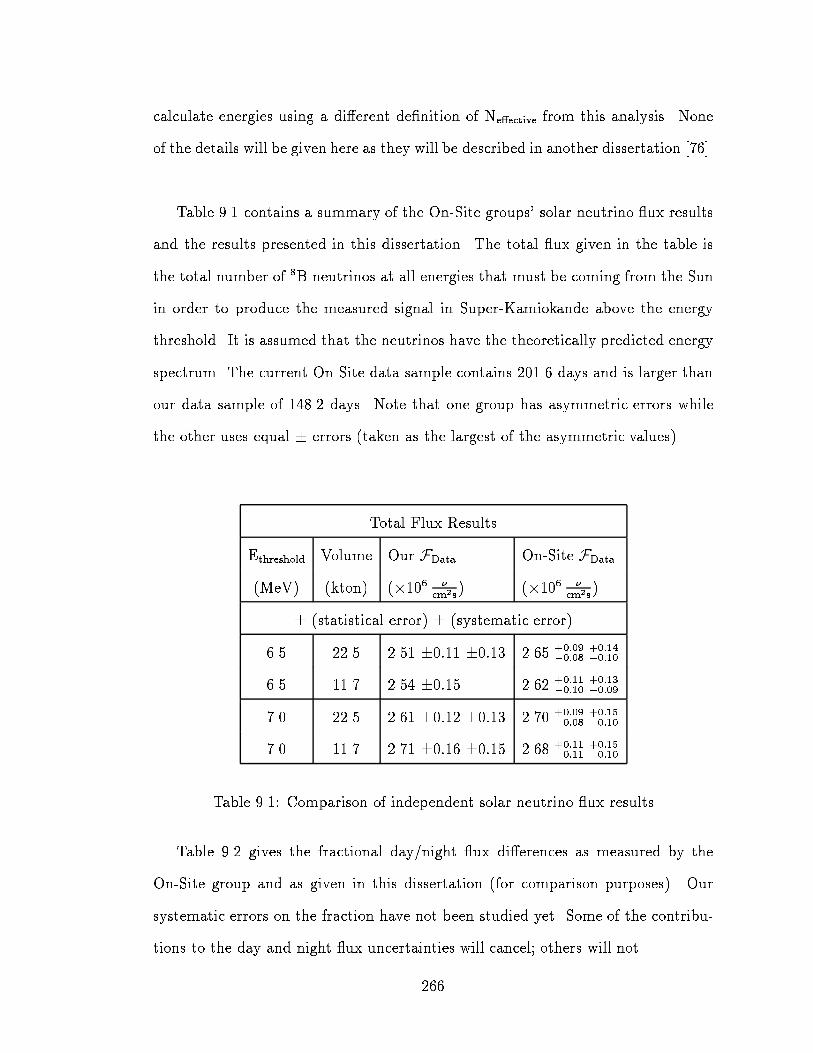
calculate energies using a di�erent de�nition of Ne�ective from this analysis. None
of the details will be given here as they will be described in another dissertation [76].
Table 9.1 contains a summary of the On-Site groups' solar neutrino ux results
and the results presented in this dissertation. The total ux given in the table is
the total number of 8B neutrinos at all energies that must be coming from the Sun
in order to produce the measured signal in Super-Kamiokande above the energy
threshold. It is assumed that the neutrinos have the theoretically predicted energy
spectrum. The current On-Site data sample contains 201.6 days and is larger than
our data sample of 148.2 days. Note that one group has asymmetric errors while
the other uses equal � errors (taken as the largest of the asymmetric values).
Total Flux Results
Ethreshold Volume Our FData On-Site FData
(MeV) (kton) (�106 �cm2s
) (�106 �cm2s
)
� (statistical error) � (systematic error)
6.5 22.5 2.51 �0:11 �0:13 2.65 +0:09�0:08
+0:14�0:10
6.5 11.7 2.54 �0:15 2.62 +0:11�0:10
+0:13�0:09
7.0 22.5 2.61 �0:12 �0:13 2.70 +0:09�0:08
+0:15�0:10
7.0 11.7 2.71 �0:16 �0:15 2.68 +0:11�0:11
+0:15�0:10
Table 9.1: Comparison of independent solar neutrino ux results
Table 9.2 gives the fractional day/night ux di�erences as measured by the
On-Site group and as given in this dissertation (for comparison purposes). Our
systematic errors on the fraction have not been studied yet. Some of the contribu-
tions to the day and night ux uncertainties will cancel; others will not.
266

Day versus Night Fluxes
Ethreshold Volume D�ND+N
(MeV) (kton) This Thesis On-Site
6.5 22.5 -0.017 � 0.047 +0.004 � 0.031 � 0.017
6.5 11.7 -0.012 � 0.059 -0.048 � 0.040 � 0.017
7.0 22.5 +0.019 � 0.046 +0.004 � 0.033 � 0.017
7.0 11.7 -0.024 � 0.058 -0.046 � 0.043 � 0.017
Table 9.2: Comparison of independent day/night ux di�erences
These ux and day/night results results and those from the On-Site group are
in good agreement. Although the two groups are using completely di�erent vertex
�tters, energy reconstruction, and event selection, getting the same answer from
both groups boosts our con�dence in the results from this experiment.
9.2 Comparison with Previous Results
In order to gauge the impact of these new solar neutrino results, a comparison is
made against the most recent published results from the Kamiokande experiment,
our predecessor. The Kamiokande results are shown in Table 9.3. Note that the
results presented in this dissertation agree with the previous results, but have much
smaller errors.
267

Previous Results from Kamiokande (680 m3)
Total Flux (E> 7 MeV) [15] 2.82 +0:25�0:24 � 0.027 �106 �
cm2s
D�ND+N (E> 9:3 MeV & E> 7:5 MeV) [77] +0.08 � 0.11 � 0.03
Table 9.3: Prior experimental solar neutrino results
9.3 Neutrino Oscillation Interpretation
One of the proposed explanations to the apparent lack of solar neutrinos is neu-
trino avor oscillations, possibly enhanced by the MSW mechanism. The basic
concepts behind neutrino oscillations and the MSW mechanism are discussed in
Section 1.6.6. Within this framework, the two oscillation parameters, sin2 2# and
�m2, determine what the measured ux should be. The most straightforward way
to �gure out which values of the parameters yield solar neutrino uxes which are
consistent with our measurement is to compute the predicted event rate in Super-
Kamiokande for every set of parameters. Allowed sets of parameters will yield
uxes within the errors on our measured ux and the SSM predictions. A contour
plot (`oscillation plot') can then be made showing the allowed regions of parameter
space.
We need to compute the predicted event rate our analysis would measure for
many di�erent sets of oscillation parameters. Our method requires the calculation
of the energy dependent �e survival probability out of the Sun (P(E�)) for each set
of mixing parameters. The survival probability can then be multiplied by the SSM
�e ux (Fssm(E�)) to yield the oscillation modi�ed �e spectrum. From this point
on, we follow the calculation described in Section 8.7. The predicted event rate
268

Rosc is:
Rosc =Z Emax
0Posc(E�)Fssm(E�)
Z Tmax
0Nelec
d�(E�; Te)
dTe�total(Te) dTedE� (9.1)
whereNelec is the number of electrons in the full inner volume of Super-Kamiokande,
d�(E� ;Te)dTe
is the di�erential cross section for scattering between a neutrino of energy
E� and an electron with kinetic energy Te, and �total is the total e�ciency including
the �ducial volume selection for an electron with kinetic energy Te to end up in the
�nal sample (given in Section 8.6). Using the above general formula and particular
survival probability functions, we will compute the expected event rates in Super-
Kamiokande for every set of oscillation parameters which we consider.
9.3.1 Vacuum Oscillations
We �rst consider vacuum neutrino oscillations. In order to calculate Rvac, we need
to determine the survival probability Pvac(E�). From Section 1.6.6, we know the
survival probability for detecting a �e with energy E� after traveling a distance r:
Pvac(�e ! �e) = 1� sin2 [2#] sin2"�m2r
4E��hc
#(9.2)
We directly use this equation to estimate the loss in the �e signal as the neutrinos
travel out of the Sun or from the Sun to the Earth. Figure 9.1 shows an example of
the energy dependence of Pvac over the solar neutrino energy range. The probability
Pvac(E�) oscillates more rapidly than the sampling energy bin size used to plot the
function; Pvac(E�) in the region below 2 MeV always oscillates between 0.4 and 1.
We use Equation 9.1, the probability Pvac(E�), and the travel distance of the
neutrino to compute Rvac. When we consider oscillations occurring inside of the
Sun, we need to remember that all neutrinos are not created at the center of the
Sun. To properly account for the range in neutrino path lengths required to exit
269

Neutrino Energy (MeV)
Vac
uum
Osc
illat
ion ν
e S
urvi
val P
roba
bilit
y
Figure 9.1: Vacuum oscillation survival probability
the Sun, we should integrate over the radial probability distribution (shown in Fig-
ure 9.2) for the 8B neutrino production. After the neutrinos leave the Sun, we
assume that they all travel the same distance before being detected on Earth. The
Earth-Sun distance changes by �2% with the Earth's location along its orbit. We
have not accounted for this variation in this calculation.
To determine the allowed regions in vacuum oscillation parameter space, we
compute Rvac(�m2; sin2[2#]) for sets of oscillation parameters. We then make a
plot showing which parameter values yield an expected ux which is within errors
of our measurement. This analysis was performed using our ux measurement cor-
responding to Ereconstruct > 7 MeV. Figures 9.3 through 9.5 show the parameter
regions allowed at the 90% con�dence level (CL) when the various errors are com-
bined together in di�erent ways. The measured ux has statistical and systematic
uncertainties. Uncertainties also exist for the predicted ux and were given in Ta-
ble 1.1 (we use the BP95 ux and corresponding uncertainties). For Figure 9.3,
we compute the 90% CL using only the statistical error on the measurement. If
270

Radius/Solar Radius
8 B ν
Pro
duct
ion
Pro
babi
lity
Figure 9.2: Radial dependence of the probability to produce a 8B neutrino
we assume that the three errors are independent and add them in quadrature, we
get the allowed region shown in Figure 9.4. If we take the worst case and add the
three errors linearly, we get the region given in Figure 9.5. Note that in much of
the parameter space shown in the Figures, the MSW e�ect must be considered.
sin22θ
∆ m
2 (eV
2 )
Figure 9.3: Allowed vacuum oscillation parameters using �stat only.
271

sin22θ
∆ m
2 (eV
2 )
Figure 9.4: Allowed vacuum osc. parameters using (�2stat + �2syst + �2theo)1=2.
sin22θ
∆ m
2 (eV
2 )
Figure 9.5: Allowed vacuum osc. parameters using (�stat + �syst + �theo).
272

9.3.2 MSW Enhanced Oscillations
The computation of the allowed regions in the oscillation parameter space for MSW
oscillations involves much more computation than the vacuum oscillation case. To
compute the survival probability Pmsw(E�), we need to numerically integrate the
time evolution of the neutrino wavefunction as it travels out of the Sun. The
wavefunction time evolution is given in Equation 1.11 with H reduced down to:
H =1
2p
m21 +m2
2
2
2664 1 0
0 1
3775� 1
2p
�m2
2
2664 A� cos 2# sin 2#
sin 2# cos 2#
3775 (9.3)
where A is the contribution to the Hamiltonian induced by the forward � � e scat-
tering (the matter term added by Wolfenstein). A is proportional to the electron
number density Ne at the location of the neutrino. Figure 9.6 shows the variation
in Ne as a function of the distance from the core of the Sun.
Radius/Solar Radius
Ele
ctro
n D
ensi
ty in
the
Sun
(1023
e /
cm3 )
Figure 9.6: Radial dependence of the electron number density
The �rst term contributes an overall phase to the wavefunction and can there-
fore be neglected from the mixing probability. To perform the actual integration,
273

we consider this to be a one-dimensional problem. It is assumed that the neutrino
traveled outwards along a radial path from the production point to the surface of
the Sun. We break up the total distance traveled into small intervals. For each
interval, we compute the change to the real and imaginary components of the mass
eigenstate wavefunctions (j�1i and j�2i). The corresponding evolution for the weakforce eigenstates (j�ei and j�xi) is computed. When the neutrino exits the Sun, we
can compute the resultant survival probability Pmsw(E�) assuming only the MSW
enhancement of the oscillations in the Sun. An example of Pmsw(E�) is given in
Figure 9.7.
Neutrino Energy (MeV)
MS
W O
scill
atio
n νe
Sur
viva
l Pro
babi
lity
Figure 9.7: MSW oscillation survival probability at the Sun's surface
After the neutrino reaches the edge of the Sun, we stop using the matter-
enhanced oscillation probability. We continue to evolve the neutrino wavefunction
assuming vacuum oscillations as the neutrino travels to the Earth. Once it arrives
at the Earth, we can compute the survival probability for the neutrino to be de-
tected in the j�ei state.
274

As with the vacuum solution, Figures 9.8 through 9.10 show theMSW parameter
regions allowed at the 90% con�dence level (CL) for di�erent error combinations.
Figure 9.8 uses only the statistical error. If we add them in quadrature, we get the
allowed region shown in Figure 9.9. For linear error addition, we get the region
given in Figure 9.10. To enable comparisons with previous experimental results
and interpretations, we also give the contours assuming the older SSM, BP92, in
Figures 9.11 through 9.13. The contours of the allowed regions implied from these
results are in good agreement with the previously published contours.
9.3.3 Di�erential Energy Spectrum
When attempting to extract the MSW parameters which best �t the di�erential
spectrum (Figure 8.11), the e�ect of the energy resolution can not be forgotten.
The combination of the SSM spectral shape and the detector resolution leads to a
di�erence in the relative shapes of the post-MSW spectrum and the SSM spectrum:
Fmsw(Egenerated)
FSSM(Egenerated)6= Fmsw(Ereconstruct)
FSSM(Ereconstruct)
The generated electron energy distributions (from both SSM and MSW a�ected
neutrinos) must be folded with the energy resolution function in order to cor-
rectly compare the predicted shape distortion with the measurement from Super-
Kamiokande.
A correct oscillation interpretation of the spectral shape of the data can not be
performed without the proper inclusion of the systematic errors. The systematic
errors on the di�erential energy spectrum have not been given in this dissertation.
The study of these systematics is ongoing. Therefore, an oscillation interpretation
of the spectrum is not presented here.
275
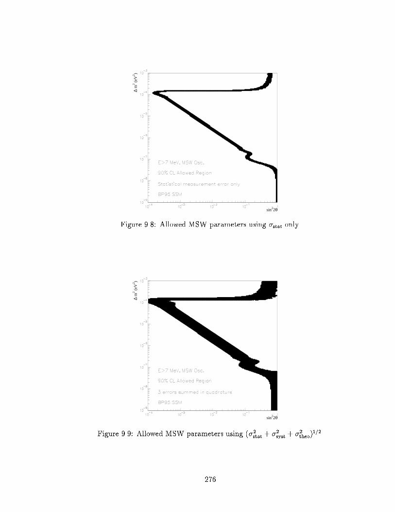
sin22θ
∆ m
2 (eV
2 )
Figure 9.8: Allowed MSW parameters using �stat only.
sin22θ
∆ m
2 (eV
2 )
Figure 9.9: Allowed MSW parameters using (�2stat + �2syst + �2theo)1=2.
276

sin22θ
∆ m
2 (eV
2 )
Figure 9.10: Allowed MSW parameters using (�stat + �syst + �theo).
sin22θ
∆ m
2 (eV
2 )
Figure 9.11: Allowed MSW parameters using BP92 and �stat only.
277

sin22θ
∆ m
2 (eV
2 )
Figure 9.12: Allowed MSW parameters using BP92 and (�2stat + �2syst + �2theo)1=2.
sin22θ
∆ m
2 (eV
2 )
Figure 9.13: Allowed MSW parameters using BP92 and (�stat+ �syst + �theo).
278

9.4 Implications
Super-Kamiokande has made a more accurate measurement of the solar neutrino
ux and has con�rmed the apparent de�cit in the total ux of neutrinos from the
Sun. The measured ux is 2.61 �0:12 (stat) �0:13 (syst) �106 �cm2s
using the data
above Ethreshold > 7 MeV. The measurement is low compared to the Standard Solar
Model calculations (BP95) of 6.62 �106 �cm2s
for the 8B ux.
It is apparent from the measured uxes from the DAY and NIGHT data sam-
ples, that we have no statistically signi�cant day/night ux di�erence. The large
angle MSW oscillation solution predicts a day/night ux di�erence (the `day/night
e�ect') which can be as large as a 50%. The current data sample does not have
the statistical accuracy to rule out the large angle solution yet. After 3 years of
operation, the statistical errors should be reduced by a factor of �2. To improve the
statistical accuracy on the day/night measurement further, work must be done to
signi�cantly reduce the background level while maintaining or increasing the total
e�ciency for saving the solar neutrino events.
The next step for Super-Kamiokande will be an in depth study of the energy
distribution of the solar neutrinos and the energy dependent systematic errors. We
can not actually measure the neutrino energies, but we measure the electron en-
ergies after the � � e scattering. We can compare the shape of the measurement
to the shape of the predicted spectrum. We would look for any visible spectral
distortions which would indicate new neutrino physics (such as MSW-enhanced
oscillations). Such a distortion is predicted by the nonadiabatic MSW avor oscil-
lation solution. No changes to the Standard Solar Model will induce a change in
the energy spectrum for the neutrinos. Unaccounted for systematics in the energy
279

scale and the energy resolution can mock the spectral distortion typically associ-
ated with neutrino oscillations. These systematics must be studied and reduced
before a meaningful interpretation of the di�erential energy spectrum measured by
Super-Kamiokande can be made. Using both the day/night ux di�erence and the
measured energy spectrum, Super-Kamiokande should provide strong evidence for
or against neutrino avor oscillations.
The other two new solar neutrino detectors, SNO and Borexino, are not yet tak-
ing data. When they turn on, what burning questions will they need to answer? A
neutral current measurement by SNO would be a powerful addition to our current
base of knowledge. SNO's neutral current measurement would explicitly measure
the total number of neutrinos (of all 3 avors) reaching the SNO detector from
the Sun. Even if Super-Kamiokande were to assert which of the possible explana-
tions to the Solar Neutrino Problem was most supported by the Super-Kamiokande
data, an independent con�rmation would still be needed to convince the world-wide
scienti�c community. SNO could provide this con�rmation by demonstrating the
fraction of neutrinos which are �e, although not in the next year or two due to their
schedule.
Borexino's measurement of the 7Be ux would directly address the \second
Solar Neutrino Problem". Prior to Super-Kamiokande results and recent theoretical
improvements to the Standard Solar Model, reasonable agreement between the
existing solar neutrino measurements seemed to require a very small or negative
ux of 7Be neutrinos. It remains to be seen if this 7Be requirement still holds when
Super-Kamiokande results are combined in with the others. Either way, Borexino
should be the �rst detector to observe the 7Be neutrinos explicitly.
280

9.5 Future Work
The results presented in this dissertation are the �rst solar neutrino results from
the Super-Kamiokande experiment. There is plenty of work still to be accomplished
and many physics studies that may be performed using the Super-Kamiokande Low
Energy data. The immediate tasks at hand are:
� Veri�cation of and improvement in the accuracy of our absolute energy cali-
bration:
The energy scale is one of the two largest contributors to the systematic
error in the ux. If we can improve the agreement between the Monte Carlo
simulation and the calibration data, we can reduce our uncertainty in the
energy scale. The contribution to the overall ux systematic error can then be
lowered. The LINAC and titanium source data will provide needed constraints
for our energy calibration.
� Investigation into a more appropriate shape for the background �t in the
cos �sun distributions for ALL, DAY, and NIGHT data samples:
We have approximated the shape of the background as a straight line which
is extrapolated under the solar neutrino peak. We know that the exposure
of Super-Kamiokande to the Sun is not the same during day and night. We
also know that we do not have an isotropic background. Obtaining the correct
functional �t to the background will require a study of the detector's exposure
to the Sun and the background distributions. By improving the shape of the
�t, we should further reduce the systematic error on the ux.
281

� Addition of reasonable cuts which remove problematic background events:
Our ability to reduce the background must improve. We will continue to
collect additional solar neutrino candidate events. We will also work to reduce
our systematic errors. The best way to improve the statistical signi�cance of
our solar neutrino signal is to improve the SignalpBackground
for our data set. We
need to lower the background level to improve the signi�cance of our signal.
� Continued re�nement of the Monte Carlo simulation program:
Recently, the High Energy Analysis group determined that some of the tuned
parameters in the Monte Carlo detector simulation did not reproduce several
important features in the high energy regime. Since both analysis groups use
a single simulation program, we must work to determine a new, improved set
of input parameters.
� Study of the allowed regions in oscillation parameter space produced by the
ALL, DAY, and NIGHT uxes:
In this dissertation, we have only discussed the parameter regions allowed by
the total ux measurement above 7 MeV. Further work should continue using
the results corresponding to other energy thresholds. Also, we should account
for the possible matter enhanced oscillations occurring near the Earth's core.
The di�erences between the day and night uxes are the key to possible
regeneration in the Earth. Excluded regions in the oscillation parameter
space based on the day/night di�erence need to be studied.
282

� Production of a solar neutrino induced electron energy spectrum with system-
atic errors relative to the expected shape from theoretical particle physics:
The spectrum is the next experimental key available to Super-Kamiokande
which may indicate the source of the apparent solar neutrino de�cit. If Super-
Kamiokande should measure a spectral distortion, new neutrino physics would
be required as an explanation. For example, a change in the spectral shape
is predicted by the nonadiabatic MSW oscillation solution. The energy de-
pendent systematic errors must be included when the spectrum shape is in-
terpreted.
� Demonstration of Super-Kamiokande's ability to properly measure an elec-
tron energy spectrum:
In order for any solar neutrino spectral measurement to be believed, we must
show our ability to correctly measure a distribution of energies from some
known sources. A comparison of the measured energy spectrum and the
expected shape for spallation products and a � decay calibration source should
prove the reliability of the measurement and analysis techniques.
283

Appendix A
Zebra Banks
The Super-Kamiokande data format is a set of zebra banks [44]. A zebra bank is
a block of information with some space set aside for `links' to neighboring zebra
banks. The rest of the space contains data in a particular format. Zebra banks are
typically created in a mother-daughter environment so that a new `child' bank is
linked with an existing `mother' bank. The routines to read, write, modify, create,
and whatever else you want to do with zebra banks were written and supported by
CERN. A map of the zebra banks in a data �le is like a road map in a big city, it
tells you where the interesting data is located. The nice thing about zebra �les is
that the directions remain constant, even if a new `street' is added along the way
to the destination. If the data was stored in an array, you would need to know if
an extra piece of information got added in the middle of the array in order to index
the array correctly. That type bookkeeping is hidden from the zebra user.
Super-Kamiokande's data contains many di�erent zebra banks. Table A.1 lists
the various banks that are found in the data, the relationship between various
banks, and what information is contained in the bank. Tables A.2 through A.6
detail the information stored in many of the banks and the type of variables which
hold that information.
284

Bank Mother Contents
EMB - Main structural link for event
HEAD EMB Header information
AHEA EMB Anti-header information
TQ EMB PMT data (On-Site format)
EVIN EMB Time of previous event
HDRI EMB PMT charge calibration information
CALI EMB Inner detector PMT data (O�-Site format)
CALO EMB Outer detector PMT data (O�-Site format)
USSK EMB Structural link for all O�-Site created banks
USMC USSK O�-Site MC information
TRAK USSK Generic track storage bank
MCPT TRAK MC particle non-track information
LEF1 USSK lef1 �lter information
THR1 USSK THR1 �t parameters
THR2 USSK THR2 �t parameters
FSTM USSK FSTMU �t parameters
HAYA USSK Hayai �t parameters
LEF2 USSK lef2 �lter information
MBOY USSK Muboy �t parameters
COMB USSK Combo�t �t parameters
CUBE USSK Cubist tag and exposures
Table A.1: Names of zebra banks and information contained in each bank
285

Field Storage Description
run mode int mode of run
run int run number
sub run int sub run number
event int event number
yr mth day int y*10000 + m*100 + d from computer clock
hr min sec int h*10000 + m*100 + s from computer clock
clock48 int[3] 48 bit clock
trg id int trigger type from TRG
trg event counter int TRG event counter
event ag int event ag
tko status int[2] TKO status
servers int[56] server (workstation) status
Table A.2: Description of HEAD bank
286
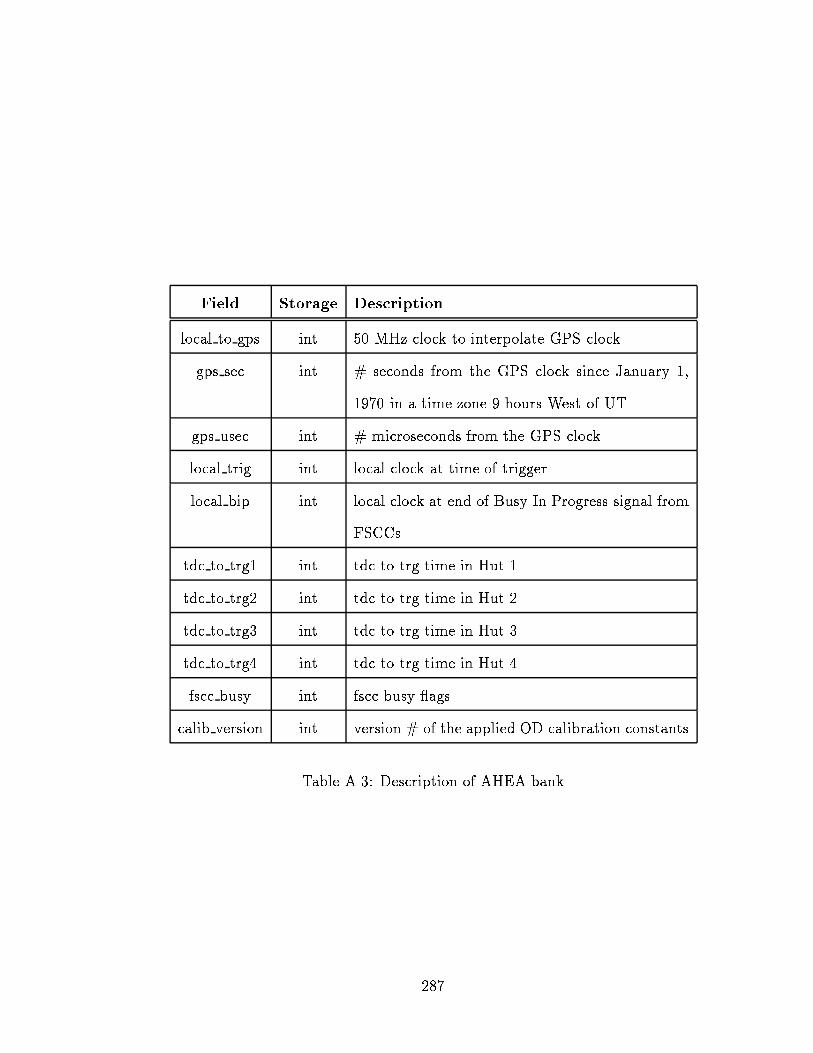
Field Storage Description
local to gps int 50 MHz clock to interpolate GPS clock
gps sec int # seconds from the GPS clock since January 1,
1970 in a time zone 9 hours West of UT
gps usec int # microseconds from the GPS clock
local trig int local clock at time of trigger
local bip int local clock at end of Busy In Progress signal from
FSCCs
tdc to trg1 int tdc to trg time in Hut 1
tdc to trg2 int tdc to trg time in Hut 2
tdc to trg3 int tdc to trg time in Hut 3
tdc to trg4 int tdc to trg time in Hut 4
fscc busy int fscc busy ags
calib version int version # of the applied OD calibration constants
Table A.3: Description of AHEA bank
287

Field Storage Description
ngood int # \good" hit tubes
nbad int # \bad" hit tubes
tube struct[ngood] PMT data
struct contains:
number int tube number
status int status word
time oat PMT time in ns
charge oat PMT charge in \photoelectrons"
Table A.4: Description of CALI and CALO banks
288

Field Storage Description
version int version # of lef1 code
cut version int version # of cut parameters
date int date lef1 was compiled
run date int date lef1 was executed on the data
class int event classi�cations from lef1
trash int tag returned from Trashman
time since ped int time [s] since end of last pedestal period
tot ID hit int total # ID PMT hits
inner max hits int max. # ID hits in 200 ns residual window
time inner maxhits oat beginning time of the 200 ns ID window
tot OD hit int total # OD PMT hits
outer max hits int max. # OD hits in 200 ns residual window
time outer maxhits oat beginning time of the 200 ns OD window
inner charge oat total charge in ID
track goodness oat goodness of �t from anis track routine
through goodness oat total time residual from THR2 �t
zenith cosine oat z direction cosine from THR2 �t
Table A.5: Description of lef1 bank
289

Field Storage Description
version int version # of lef2 code
cut version int version # of cut parameters
date int date lef2 was compiled
run date int date lef2 was executed on the data
class int event classi�cations from lef2
class same as lef1 int ag = 1 if class has not changed from lef1
goodbad int good&bad data ag for subrun
minbias int ag = 1 if minimum bias event
upgoing int ag = 1 if upgoing muon event
time since mu oat time in �s since the last muon
Table A.6: Description of lef2 bank
290

References
[1] J. Bahcall, Neutrino Astrophysics, Cambridge University Press, Cambridge,
1989.
[2] See for example [4] or S. Turck-Chi�eze and I. Lopes, Astr. Jour., 408, 347
(1993).
[3] Totsuka, Y., University of Tokyo (ICRR) Report ICRR-Report-227-90-20
(1990).
[4] J. Bahcall and M. Pinsonneault, Rev. Mod. Phys., 67, 781 (1995).
[5] J. Bahcall and R. Ulrich, Rev. of Mod. Phys., 60, 297 (1988).
[6] W. F. Huebner, et.al., \Astrophysical Opacity Library," Los Alamos Scienti�c
Laboratory Report No. LA-6760-M, 1977.
[7] J. Bahcall and M. Pinsonneault, Rev. Mod. Phys., 64, 885 (1992).
[8] R. Davis Jr., Phys. Rev., 97, 766 (1955).
[9] J. Bahcall and R. Davis Jr., Essays in Nuclear Astrophysics, Cambridge Uni-
versity Press, Cambridge, 1982.
[10] R. Davis Jr., D. Harmer, and K. Ho�man, Phys. Rev. Lett., 20, 1205 (1968).
291

[11] J. K. Rowley, B. T. Cleveland, and R. Davis Jr., Proc. Conf. on
Solar Neutrinos and Neutrino Astronomy (Homestake, S.D. 1984), eds.
M. L. Cherry, K. Lande, and W. A. Fowler, AIP Conf. Proc. 126 (AIP, New
York, 1985)
[12] B.T. Cleveland et.al., Nucl. Phys. (Proc. Suppl.), B38, 47 (1995).
[13] K. S. Hirata et.al., Phys. Rev., D44, 2241 (1991).
[14] K. Inoue, Ph.D. Thesis, Univ. of Tokyo (1993).
[15] Y. Fukuda et.al., Phys. Rev. Lett., 77, 1683 (1996).
[16] A. Abazov et.al., Phys. Rev. Lett., 67, 3332 (1991).
[17] P. Anselmann et. al, Phys. Lett., B285, 376 (1992).
[18] R. Wink et.al., NIM, A329, 541 (1993).
[19] GALLEX Collaboration, Phys. Lett., B327, 377 (1994).
[20] J. N. Abdurashitov et.al., Nucl. Phys. (Proc Supp.), B38, 60 (1995).
[21] N. Hata, S. Bludman, and P. Langacker, Phys. Rev., D49, 3622 (1994).
[22] V. Castellani et.al., Phys. Rev., D50, 4749 (1994).
[23] V. Castellani, S. Degl'Innocenti, and G. Fiorentini, Astr. Astrophysics, 271,
601 (1993).
[24] C. Arpesella, Nucl. Instr. and Meth., A350, 327 (1994).
[25] P. Anselmann et.al., Phys. Lett., B342, 440 (1994).
[26] A. Cumming and W. Haxton, Phys. Rev. Lett., 77, no. 21, 4286 (1996).
292

[27] L. Wolfenstein, Phys. Rev., D17, 2369 (1978).
[28] S. P. Mikheyev and A. Y. Smirinov, Nuov. Cim., 9, 17 (1986).
[29] T.K. Kuo and J. Pantalone, Rev. Mod. Phys., 61, 937, (1989).
[30] N. Hata and P. Langacker, Phys. Rev. D, 50, 632 (1994).
[31] G. T. Ewan et.al., \Sudbury Neutrino Observatory Proposal," Report No.
SNO-87-12 (1987) (unpublished).
[32] T. Kovacs et.al., Solar Phys., 128, 61 (1990).
[33] D. Chen, private communication.
[34] Y. Fukuda et.al., \Development of the Data Acquisition System for Super-
Kamiokande," Super-Kamiokande Report SKAM-95-03 (1995).
[35] R. Claus et.al., NIM, A261, 540 (1987).
[36] A. T. Suzuki et.al., \Improvement of 20-Inch Diameter Photomultiplier
Tubes," KEK Preprint 92-50 (1992).
[37] Y. Fukuda et. al., \Development of the Data Acquisition System for Super-
Kamiokande," Super-Kamiokande Report SKAM-95-03 (1995).
[38] M. Shiozawa, M.S. Thesis, Univ. of Toyko (1994).
[39] TKO Speci�cations, KEK Report 85-10, November 1985.
[40] J. Flanagan and M. Masuzawa, \Study of Super-Kamiokande Inner Detector
Front End Electronics," (1994).
[41] LeCroy spec sheet at http://www.lecroy.com/, April 1996.
293

[42] Z. Conner et. al., \Monte Carlo Results of Trigger Schemes," Super-
Kamiokande Report SKAM-93-03 (1993).
[43] M. Shiozawa, personal communication.
[44] \Zebra, Overview of the ZEBRA System," CERN Program Library Q100 and
Q101 (1995).
[45] T. Haines, Z. Conner, et.al., \Super-Kamiokande Calibration: An Interim Re-
port," (1994).
[46] See the Super-Kamiokande Collaboration Meeting Notes from November 1995,
April 1996, and July 1996 for descriptions of the xenon calibration system.
[47] Z. Conner et.al., \Status Report of Laser Calibration System," (1995).
[48] K. Inoue, Ph.D. Thesis, Univ. of Tokyo (1993).
[49] H. S. Park, Ph.D. Thesis, University of Michigan (1985).
[50] A. Melissinos, Experiments in Modern Physics, Academic Press Inc., New
York, 1966.
[51] Nucl. Data Tables, A3, 369 (1969).
[52] Neutron Sources: For Basic Physics and Applications, Pergamon Press, New
York, 1983, p. 7.
[53] K. Inoue and Y. Suzuki, \Improvement of Ni(n, )Ni' Calibration Source for
the Delayed Coincidence Method," Super-Kamiokande Report SKAM-94-07
(1994).
[54] J.F. Briesmeister, \MCNP: A General Monte Carlo N-Particle Transport
Code," LA-12625-M.
294

[55] M. Nakahata and K. Nishikawa, \Electron LINAC for the Calibration of Super-
Kamiokande," Super-Kamiokande Report SKAM-93-04 (1993).
[56] M. Morita, Beta Decay and Muon Capture, W.A. Benjamin, Inc., Reading,
Massachusetts, 1973, p. 276.
[57] T. Suzuki, D.F. Measday, and J.P. Roalsvig, Phys. Rev., C35, 2212 (1987).
[58] E.K. Warburton, D.E.Alburger, and D.J. Millener, Phys. Rev., C29, 2281
(1984).
[59] J.N. Bahcall et.al., \Standard Neutrino Spectrum from 8B Decay," IASSNS-
AST 95/47.
[60] L. B. Okun, Leptons and Quarks, North-Holland Publishing Company, New
York, 1982, p. 138.
[61] W.R. Nelson, H. Hirayama, and D.W.O. Rogers, \The EGS4 Code System,"
SLAC-Report-265 (1985).
[62] D.W.O. Rogers, NIM, 227, (1984) 535.
[63] Z. Conner, \Low Energy Electrons With EGS4," Super-Kamiokande Report
SKAM-93-02 (1993).
[64] \GEANT Detector Description and Simulation Tool," CERN Program Library
W5013 (1994).
[65] R.C. Smith and K.S. Baker, Appl. Opt., 20, 177 (1981).
[66] J.D. Jackson, Classical Electrodynamics, John Wiley and Sons, New York,
1975.
[67] F. Goebel, M.S. Thesis, State Univerity of New York at Stony Brook (1996).
295

[68] H. Press et.al., Numerical Recipes in Fortran, Cambridge University Press,
New York, 1992.
[69] \PAW - Physics Analysis Workstation," CERN Program Library Q121 (1995).
[70] \HBOOK Reference Manual," CERN Program Library Y250 (1995).
[71] R. Firestone, Table of Isotopes, John Wiley & Sons, Inc., New York, 1996.
[72] M. Nakahata, Ph.D. Thesis, University of Tokyo (1988).
[73] K. Matsumoto and Y. Suzuki, \Measurement of Rn originating from the
20inch PMT glass and other materials used i the Super-Kamiokande," Super-
Kamiokande Report SKAM-94-03 (1994).
[74] Y. Oyama, Kamiokande Internal memo (1984).
[75] J.N. Bahcall, M. Kamionkowski, and A. Sirlin, Phys. Rev., D51, 6146 (1995).
[76] Y. Koshio, Ph.D. Thesis, University of Tokyo (soon to be completed).
[77] K.S. Hirata et.al., Phys. Rev. Lett, 66, 9 (1991).
296