yardstick competition for service systems
TRANSCRIPT

Yardstick Competition for Service Systems
Nicos Savva · Tolga TezcanLondon Business School, Regent’s Park, London NW1 4SA, UK
[email protected] · [email protected]
Ozlem YildizUniversity of Rochester, Simon Business School
Yardstick competition is a regulatory scheme for local monopolists (e.g., hospitals), where the monopolist’s
reimbursement is linked to her performance relative to other equivalent monopolists. This regulatory scheme
is known to work well in providing cost-reduction incentives and serves as the theoretical underpinning
behind the hospital prospective reimbursement system used throughout the developed world. This paper uses
a game-theoretic queueing model to investigate how yardstick competition performs in service systems (e.g.,
hospital emergency departments), where, in addition to incentivizing cost reduction, the regulator’s goal is
to provide incentives to reduce customers’ waiting times. We first show that the form of cost-based yardstick
competition used in practice results in inefficiently long waiting times and may also lead to inefficiently high
costs. We then demonstrate how yardstick competition can be appropriately modified to achieve the dual
goal of cost and waiting-time reduction. In particular, we show that full efficiency (first-best) can be restored
if the regulator makes the providers’ reimbursement contingent on their service rates and is also able to
charge a provider-specific “toll” to consumers. If such a toll is not feasible, as may be the case in healthcare,
we show that an alternative waiting-time-based version of yardstick competition can significantly improve
system efficiency (second-best), and it is also easier to implement, as does not require the regulator to have
detailed knowledge of the queueing discipline. We conclude with a detailed numerical analysis that provides
insights on the practical implementation of yardstick competition in the healthcare industry.
Key words : Yardstick competition, hospital regulation, emergency care, game theory, queueing theory.
History : December 15, 2016
1. Introduction
Services constitute a large part of the developed world economy, and in some cases, they operate
as regulated monopolies. A case in point is the hospital industry, which in 2014 constituted 5.6%
of the US economy, and is highly regulated by bodies such as the Centers for Medicare and Medi-
caid (CMS), which are responsible for approximately 45% of hospital reimbursement(CMS 2014).1
Despite this, academic research on the regulation of service monopolies has not received as much
attention as that of “production” monopolies, e.g., defense systems, water, and energy (Laffont
and Tirole 1993, Roques and Savva 2009).
1 In other developed world healthcare systems, such as the UK, hospitals are just as large as a part of the nationaleconomy and most of their reimbursement comes from a single government-funded payer that acts as the regulator.
1

2 Savva, Tezcan, Yildiz: Yardstick Competition for Service Systems
This paper focuses on a specific regulatory scheme, yardstick competition, in which the regu-
lator induces artificial competition between local monopolists by rewarding firms on the basis of
their performance relative to each other. Yardstick competition has been shown to provide incen-
tives for monopolists to minimize production costs (Shleifer 1985) and has been widely applied to
the reimbursement of regulated utilities (e.g., electricity (Jamasb and Pollitt (2000)) and tertiary
care (through CMS’s Diagnosis-Related Group (DRG) prospective reimbursement in the US and
equivalent schemes in other developed economies (Fetter 1991)). This paper shows that yardstick
competition fails to incentivize investment in wait-time reduction in service systems. In fact, this
may be a contributing factor to the undesirably long waiting times observed in some some ser-
vice systems, such as hospital care (Government Accountability Office 2009), that are reimbursed
through yardstick competition. To incentivize waiting-time reduction through capacity investment
or process re-engineering, without compromising incentives for cost control, the yardstick compe-
tition scheme must be modified. This paper proposes one such modification.
What is yardstick competition? Historically, franchised monopolies had been subject to
“cost-of-service” regulation, where the regulated firm’s price is set equal to the (marginal) cost
of production, along with a transfer payment, if needed, to ensure the monopolist breaks even.
The fee-for-service reimbursement model, which had been used by CMS in reimbursing US-based
hospitals up to 1983 is one such example (Mayes 2007). Besides simplicity, the advantage of this
regulatory scheme is that it avoids the higher monopoly price and the associated welfare loss,
whilst providing incentives for the firm to continue production. The disadvantage is that it does
not provide incentives to minimize the cost of production.
A better alternative would be to dissociate the firm’s price from the firm’s cost of production,
and instead set it equal to an exogenous benchmark. Setting this benchmark optimally, however,
would require the regulator to know as much about the available cost-reduction technologies as the
regulated firm. Yardstick competition gets around this difficulty by making use of the production
cost of other equivalent monopolists to infer a firm’s attainable costs, which will then serve as
the exogenous benchmark. For example, the regulator could choose to reimburse the monopolist
at the average production cost of all other monopolists. By doing so, the regulator forces the
firms to engage in a cost-reduction competition, akin to a tournament, which, as shown in Shleifer
(1985), has (under mild conditions) a unique symmetric Nash equilibrium that leads to first-best
outcomes, i.e., it achieves the same cost-reduction investment as that chosen by the regulator under
full information. Since the price is set through observable and verifiable benchmarks, this scheme
can be implemented using accounting data without requiring symmetric information between the
regulator and the regulated firms.

Savva, Tezcan, Yildiz: Yardstick Competition for Service Systems 3
Yardstick competition in services. While the economic rationale behind yardstick competi-
tion is sound, the theory outlined above abstracts away one important aspect of service provision:
waiting times. Effectively, it assumes that production is instantaneous, or equivalently, that con-
sumers’ cost of waiting is negligible. This assumption may fit product-based monopolies, but it is
less realistic for service settings where long waiting times are costly and, as in the case of hospital
Emergency Departments (EDs), even dangerous. It is, therefore, important that, in addition to
cost reduction, the regulation of service systems should also incentivize wait-time reduction.
To do this we present a game theoretic queueing model of yardstick competition, where a reg-
ulator is responsible for multiple identical service providers that act as local monopolists. The
regulator’s objective is to maximize total welfare by dictating the price that customers are charged
and any transfer payments made to the service providers. Service providers are assumed to be
profit maximizers and, given the price and transfer payment set by the regulator, decide how much
to invest in cost- and wait-time-reduction effort. Finally, customers are heterogeneous in their will-
ingness to pay for the service leading to an endogenous demand function that is decreasing in both
the price, as well as the waiting time they expect to incur. A crucial feature of our model, which
explains why optimal regulation may be difficult, is that the providers’ cost technology and the
customer demand function are not known to the regulator. We note that extant models that ignore
the cost of waiting (e.g., Shleifer 1985) are a special case of the model presented here.
Using this model, we show that in contrast to product-based monopolies, applying the standard
cost-based yardstick competition scheme to service monopolies results in inefficiently long waiting
times, and may even result to inefficiently high costs due to two types of inefficiencies. First,
customers will over-join the service system compared to first-best, a result first noted in Naor
(1969). This is due to a negative externality: a customer’s decision to join the system will lead to
an increase in the expected waiting time of others. Nevertheless, this increase does not feature in
his personal calculation as to whether to join the system or not. Second, the cost-based yardstick
competition fails to generate incentives for the service providers to increase capacity.
To resolve these two inefficiencies, i.e., incentivize optimal customer joining behavior and ade-
quately incentivize waiting-time reduction, yardstick competition should be modified in two ways.
First, the price that customers pay to access the service should be higher than the costs of service
production estimated through the yardstick competition benchmarks. This higher price constitutes
a form of “toll” and is equal to the displaced utility that a customer’s joining decision generates
(Naor 1969). Second, the monopolists’ reimbursement should have a component that depends on
their investment in wait-time reduction. More specifically, the monopolist’s reimbursement should
include a component that depends on the difference between her service rate and the average ser-
vice rate of all other monopolists that serve as the benchmark. This modified yardstick competition

4 Savva, Tezcan, Yildiz: Yardstick Competition for Service Systems
achieves first-best outcomes on both cost and waiting-time reduction and, just like the cost-based
yardstick competition, can be implemented using accounting data on costs and waiting times, along
with some information on the queueing discipline.
An essential feature of the yardstick competition scheme discussed above is that customers are
charged a provider-specific fee for accessing the service. In many healthcare settings, this is not the
case; care is either free at the point of access, or patients are charged a fixed insurance deductible.
We show that if customers are charged an exogenous fee (which could be zero) then there is
an inefficiency due to the suboptimal customer joining behavior. Nevertheless, there exists an
alternative yardstick competition scheme that still achieves second-best, i.e., there is no additional
loss of welfare due to underinvestment in either cost or waiting-time reduction. Furthermore, this
scheme also attenuates the regulator’s information requirements – the regulator needs to observe
the customer waiting time and total provider costs, but does not need to know anything about the
queueing discipline or how the costs are split between fixed and variable.
Finally, we present a series of extensions that explain how yardstick competition can be imple-
mented in settings with multiple customer classes, time-varying arrival rates, more general cost
structures and discuss how the regulator could adjust the yardstick competition scheme to account
for heterogeneity between the local monopolists based on exogenous and observable characteristics.
We also present a detailed numerical analysis that investigates the magnitude of the welfare loss
associated with second-best outcomes compared to fist-best, and the dependance of the equilibrium
outcome on the cost of waiting. One interesting finding is that, in contrast to equilibrium waiting
times, total welfare is not very sensitive to the cost-of-waiting parameter. This suggests that the
service provider may be able to use the cost-of-waiting parameter as a lever to shift the equilibrium
outcome associated with the modified yardstick competition to one with lower waiting times at the
expense of higher costs.
Yardstick competition and hospital reimbursement. One immediate application of the
modified yardstick competition model proposed by this paper is the regulation of hospital EDs.
First, hospitals act, to a large extent, as local monopolists, as patients do not (or cannot) shop
around for hospital care (Thomson 1994, Wang et al. 2016). Second, hospitals in general, and
EDs in particular, are comparable in the sense that the medical “technology,” which is based on
the existing understanding of biology, pharmacology, physiology etc., is not hospital specific and
neither is the waiting-time reduction “technology.” Furthermore, any differences between hospitals,
such as labor costs, case mix, and size of catchment area, are readily observable and exogenous.
These two reasons explain why yardstick competition has been widely adopted around the world

Savva, Tezcan, Yildiz: Yardstick Competition for Service Systems 5
as a form of regulation for this industry.2 Third, waiting time to receive emergency care is both
costly and, in many cases, excessively long.3
This paper provides an explanation as to why there is such a systematic underinvestment in
reduction of waiting times in emergency care. It also provides guidelines on how regulators could
modify the reimbursement system already in use to provide incentives for waiting time reduction.
More specifically, the second-best scheme that we propose is particularly useful, as it requires little
additional information to implement (just average waiting time at the ED)4 and achieves outcomes
that cannot be improved upon without changing the way that patients are charged for accessing
emergency care.
Beyond healthcare and hospital reimbursement, our work serves as an introduction to
the notion of yardstick competition to the operations management community. More specifically,
yardstick competition might be a useful tool for other service systems that operate as local monop-
olies (e.g., governmental agencies, such as the Department of Motor Vehicles and Social Security
offices in the US; (former) quasi-state monopolies, such as the post office; airport or border secu-
rity checkpoints), as well as within a service firm to incentivize better performance for individual
servers.
2. Literature Review
The observation that relative-performance evaluations is a useful tool for setting incentives has
been made by Holmstrom (1982), Nalebuff and Stiglitz (1983), and Shleifer (1985) in related
2 The form of yardstick competition used in hospital reimbursement is based on the work of Professor Fetter andco-authors in the 1970-80s, which classifies acute patients into Diagnosis-Related Groups (DRGs) based on theirdiagnosis, existing complications and comorbidities, and patient-specific characteristics, e.g., age (see Fetter (1991)).The classification is done so that patient episodes within a group will require a homogeneous bundle of services andgoods to be diagnosed and treated, and should therefore cost the same irrespective of where this treatment takesplace. Hospitals are then reimbursed a fixed amount per patient that depends only on the patient’s DRG. The amountis set to the average of the reported (and audited) cost of treating patients of the same DRG in other hospitals(subject to adjustments based on exogenous hospital characteristics). Since its introduction by CMS in the US inthe 1980s, the system has been adopted by private insurance firms and healthcare payers throughout the developedworld.
3 According to the US Government Accountability Office, the most urgent patients who should have been seen in lessthan 1 minute waited for 28 minutes on average, and the emergent patients who are recommended to be seen in lessthan 14 minutes waited an average of 37 minutes (Government Accountability Office 2009). Similarly, ED wait timesin England have risen by one third in November 2015 compared to November 2014 (Siddique 2016) and one out of 10patients spend at least eight hours in Canadian EDs (Canadian Institute for Health Information 2012). Furthermore,delays in the ED have been associated with a number of adverse outcomes, such as patient dissatisfaction, higher ratesof medical errors, higher mortality rates, and more patients leaving without receiving treatment (Batt and Terwiesch2015).
4 In fact, regulators around the world have started collecting waiting-time data. For example, Monitor, the UK hospitalregulator, collects data on ED waiting times and has placed an ad-hoc target that at least 95% of patients have to beadmitted or discharged within 4 hours of arriving to the ED with financial penalties for failure to comply (Campbell2016). Similarly, CMS has started collecting data on ED waiting times, which are reported on the Hospital Comparewebsite (CMS 2016b).

6 Savva, Tezcan, Yildiz: Yardstick Competition for Service Systems
contexts: the first focuses on curbing free-riding in teams, the second on optimal risk-sharing, and
the third on cost-cutting incentives for regulated firms. In fact, the term “yardstick competition” is
used by Shleifer (1985) to describe this form of regulation. From a practical perspective, yardstick
competition has been implemented in some industries (e.g., electricity (Jamasb and Pollitt 2000),
water and sewage (Sawkins 1995)) and has been used to generate insights on the structure and
fiscal policy of government in democratic countries (Besley and Case 1995, Bordignon et al. 2003).
Several extensions to the model of yardstick competition for regulation have been presented in
the literature. For example, Laffont and Tirole (1993), p. 84-86 augment the model of yardstick
competition to regulate firms whose costs are imperfectly correlated. Sobel (1999) examines the
case where transfers are costly to show that yardstick competition may discourage investment. This
setting has been examined further in Dalen (1998) and more recently Lefouili (2015). More relevant
to our work are models that use yardstick competition to incentivize improvements in additional
dimensions of performance, such as quality. Examples include Ellis and McGuire (1986), Pope
(1989), Ma (1994), and Tanger̊as (2009), where the general finding is that quality is better served
by more complicated forms of yardstick competition. Our work adds to this literature because
unlike quality, i) waiting times are endogenous to customer behaviour and generate an externality
on the customer side: a customer’s decision to visit a service provider increases waiting times which
places a negative externality on all other customers who join after her (see also Naor (1969)); ii)
waiting times are governed by well-understood non-linear dynamics that need to be accounted for;
iii) waiting times are often easier to quantify and less controversial to compare across providers
than other quality measures (e.g., in-hospital mortality).
In addition to the literature on yardstick competition, this paper also contributes to the opera-
tions management (OM) literature that examines incentives and competition in queueing systems.
Traditionally, queueing theory, which is well surveyed in Kleinrock (1975), has been concerned with
the mathematical description and optimization of queueing systems without considering customer
behavior or agency issues on behalf of firm management. Early attempts to include such economic
considerations are well-reviewed by Hassin and Haviv (2003), while more recent work is presented
in Hassin (2016). Our work brings together elements from i) the literature on strategic customer
behavior in monopolistic queueing systems, which was first studied in Naor (1969) for observable
queues and extended to unobservable queues by Edelson and Hilderbrand (1975) and multiclass
queues by Mendelson and Whang (1990) and Afeche (2013); and ii) the literature on queueing
games where service providers compete based on price and congestion (e.g., Cachon and Harker
(2002), Cachon and Zhang (2006), Allon and Federgruen (2007) and Allon and Federgruen (2008)).
Closest to our work are the studies of queuing games in the context of hospital/ED congestion.
An early example is Lee and Cohen (1985) which studies a setting where agents (e.g., physicians)

Savva, Tezcan, Yildiz: Yardstick Competition for Service Systems 7
direct customers to multiple service providers (e.g., hospitals) as a non-cooperative queuing game
where congestion at each service provider plays the role of prices. They show that the equilib-
rium outcome will, in most cases, entail loss of efficiency. More recently, literature has examined
resource pooling though ambulance diversion as a non-cooperative queueing game between com-
peting EDs (see Deo and Gurvich (2011) and Do and Shunko (2016)). They show that there exist
equilibria where diversions are not used optimally and propose alternative policies that are Pareto-
improving. In contrast to this stream of literature, in our setting service providers do not compete
directly. Instead, competition is induced by the regulator through the reimbursement mechanism.
Furthermore, our work is complementary to the aforementioned papers on ambulance diversion, as
it focuses on hospital reimbursement mechanisms that incentivize optimal investment in capacity,
which, as a side-effect, may make the need to divert ambulances less prevalent.
Our work is also related to the OM literature on performance-based incentives in services in
general (Akan et al. 2011, Bakshi et al. 2015, Hasija et al. 2008, Kim et al. 2007, Kim et al. 2010, Ren
and Zhou 2008) and in healthcare specifically (So and Tang 2000, Jiang et al. 2012, Lee and Zenios
2012, Adida et al. 2016, Guo et al. 2016, Andritsos and Aflaki 2015, Jiang et al. 2016). The last two
papers also consider direct competition between providers (i.e., a queueing game) in the presence
of performance-based incentives. Our paper differs, as the performance-based incentives that we
consider are not set exogenously by the regulator, but are the result of endogenous benchmarks.
This is an important difference because it generates (indirect) competition between otherwise
monopolistic providers and, as we show in this paper, may be easier to implement, as it places less
onerous informational burden on the regulator.
3. Model Description
The model of this paper considers the interaction between three parties: the regulator, the service
provider, and the customers. The regulator has N ≥ 2 identical service providers (or firms) under his
jurisdiction and has the ability to set the price that customers are charged and may also decide to
award an additional transfer payment to the service providers, which may depend on any observable
and verifiable quantity. Customers observe how much they need to pay for service and make a
decision as to whether to request service, which is provided on a-first-come-first-served basis. As a
result, customers may experience a costly wait, which we model explicitly using queueing theory.
Finally, the service providers act as risk-neutral local monopolists. They observe the price and
transfer payment set by the regulator and, given customer behavior, decide how much to invest
in cost- and wait-time-reduction effort. We present the details of the decisions and payoffs of each
of the three parties and discuss how our model applies to the hospital emergency care setting in
§§3.1-3.3.

8 Savva, Tezcan, Yildiz: Yardstick Competition for Service Systems
3.1. Service Environment, Customer Utility and Equilibrium Arrival Rate
We assume that within the catchment area of each service provider, there is a large population of
customers who may experience a service need with an exogenous probability. The aggregate arrival
rate of service needs may then be modeled as a Poisson process with rate Λ per unit time (even if
customers are strategic, see Lariviere and Van Mieghem (2004)). Each customer with a service need
makes a decision whether to visit the service provider to receive service on a first-come-first-served
basis, or use their outside option which, without loss of generality, we assume has value of zero. In
the case of emergency care, these assumptions reflect the case where patients have a single ED that
they would consider visiting, either due to prohibitive transportation costs, informational frictions,
or idiosyncratic preferences for a specific ED, e.g., the closest (Brown et al. 2015). In this case, Λ
would reflect the number of patients per unit time that exhibit a symptom (e.g., chest pain) for
which they would consider visiting the ED. Since the patients exhibit the same symptom, they
would all be classified in the same triage category; therefore, first-come-first-served is a reasonable
assumption. (We present an extension to multiple customer classes and non-stationary arrivals in
§5.1). If patients choose not to visit the ED, their outside options could be to use primary care or
not to seek treatment.
Each customer’s utility from receiving service comprises of three components. The first is the
benefit from the service r, which is net of any indirect costs associated with the service (e.g., net
of transportation costs). We assume the value of service r to be heterogeneous across customers.
The proportion of customers who value the service less than x≥ 0 is given by Θ(x). By definition,
Θ(x) is non-negative and increasing. We also assume that its derivative, which we denote with θ,
is strictly positive everywhere in [0,∞).5 In the ED setting, the benefit r denotes the value that
patients place on treatment and it is natural to assume that it heterogeneous across patients due
to the variability in the severity of patients’ conditions, which is present even within the same
triage category. The second component of customers’ utility is the price of the service, p. In the
ED setting, this may reflect the co-payment for an ED visit, which may well be zero. The third
component is the cost of waiting to receive service, which we assume to be t per unit time. In
general, it reflects opportunity cost and in the ED setting in particular, it may also reflect the
monetary value of the anxiety, pain, and inconvenience that patients might experience until they
are diagnosed and/or treated. We assume heterogeneity in this cost to be less pronounced than
that in the benefit from receiving the service and, for tractability purposes, we model this as
homogeneous across customers.
5 To avoid subtle technical questions and to facilitate game-theoretic analysis, we assume that all functions definedare twice differentiable.

Savva, Tezcan, Yildiz: Yardstick Competition for Service Systems 9
More formally, the utility that each customer expects to receive from seeking service is given by
r− tW (λ,µ)−p, where W (λ,µ) denotes the expected waiting time given the number of customers
arriving to the service provider λ and the actions of the service provider that result in increasing
throughput, which are summarized by the variable µ (see also §3.2). Throughout, we assume that
W (λ,µ) is increasing in λ and decreasing in µ. Any customer with positive utility will decide to
seek service and the equilibrium arrival rate λ(p,µ) is given by the solution of the equation
λ(p,µ) = ΛΘ̄ (p+ tW (λ(p,µ), µ)) , (1)
where Θ̄(r) := 1−Θ(r) and λ(p,µ)<µ. If, for example, the service is provided in an M/M/1 queue,
this equation reduces to
λ(p,µ) = ΛΘ̄
(p+
t
µ−λ(p,µ)
). (2)
We note that the formulation above assumes that customers do not observe the actual waiting
time when they make the decision to seek service. This is consistent with many practical settings
including EDs where patients have little visibility on actual waiting times before they visit the ED
(see Chapter 3 of Hassin and Haviv (2003) for an excellent review of the literature on unobservable
queues and its applications, and Anand et al. (2011), Rajan et al. (2014) for more recent examples).
Nevertheless, customers are assumed to have accurate beliefs about expected waiting times, W ,
which they may have formed trough repeated interactions with the service provider or word-of-
mouth.
3.2. Service Provider’s Profit and Actions
We next discuss the profit maximization problem of one service provider of the N identical service
providers. The provider is assumed to know the customers’ equilibrium arrival rate. For simplic-
ity, and in order to generate results that are comparable with extant literature, we present a
single-period model where the reimbursement mechanism, which consists of a customer price p
and transfer payment T , is set by the regulator at the beginning of the period. The duration of
this period is much longer than the average patient-interarrival time. Given the reimbursement
mechanism and the customers’ equilibrium arrival rate λ(p,µ) given in (1), the service provider’s
profit per unit time (thought the time period) is given by
Π(c,µ|p,T ) = (p− c)λ(p,µ)−R(c,µ) +T, (3)
where c is the cost of providing service per customer and µ represents the level of effort that the
service provider chooses to exert in order to reduce waiting time. The cost function R(c,µ) denotes
the cost of all activities undertaken by the service provider to reduce the cost of providing service

10 Savva, Tezcan, Yildiz: Yardstick Competition for Service Systems
to the level c and the cost of effort µ associated with reducing the waiting time. We assume that
cost R(c,µ) is a fixed cost, at least in the short-run, and it is decreasing in the cost per customer
c, increasing in effort µ, and it is jointly convex.
In the case of the ED, the single period of time may represent a year within which the regulator
has committed not to make any further adjustments to the regulatory environment. The cost per
customer c represents the overall cost of treating a patient with a specific condition and R(c,µ)
denotes the cost (per unit time) of any interventions or process re-engineering that may yield a
more cost-efficient process or increase in throughput. For instance, purchasing capital intensive new
equipment that allows for more precise and faster patient treatment, employing more and better-
qualified staff, and/or re-engineering processes (e.g., having patients triaged and diagnosed by more
experienced health care providers (Saghafian et al. (2014)), can reduce the cost of treating patients
and simultaneously increase the throughput (see Saghafian et al. (2015) for more on throughput
improvements in EDs.) We extend this model to more general cost structures in §5.2. If the service
is provided in an M/M/1 queue, the variable µ can be interpreted as the service rate (or service
capacity) of the system and, for this reason, we will refer to µ as effort or capacity interchangeably.
At the beginning of the period, the provider chooses her optimal cost c and waiting time reduction
effort µ by solving the profit maximization problem
maxco≥c>0,µ≥µo>0
Π(c,µ|p,T ). (4)
We assume that the service provider must choose the cost per patient c from the interval [0, co] and
the capacity level µ from the interval [µo,∞). The limits c0, which can be arbitrarily large, and
m0, which can be arbitrarily small, can be thought of as the (exogenous) default cost and capacity
decisions of the provider. The objective of profit maximization is not inconsistent with hospital
care, see for example the discussion in Andritsos and Aflaki (2015).
Finally, we note that in our model there exist N providers who we assume are identical in terms
of their profit function. We extend our analysis to heterogenous providers in §5.4.
3.3. Regulator’s Welfare
The regulator has the authority to dictate the price p paid by customers, the transfer payment T
received by the providers and may also choose to dictate the cost c and capacity µ set by the service
provider. These are chosen at the beginning of the time horizon in order to maximize total welfare,
which comprises the accumulated customer surplus and the profits of each of N service provider.
The expression for the total welfare rate associated with one such service provider is given by
S(p, c,µ) = Λ
∫ ∞p+tW (λ,µ)
(x− p− tW (λ,µ))dΘ(x) + (p− c)λ(p,µ)−R(c,µ), (5)
Savva, Tezcan, Yildiz: Yardstick Competition for Service Systems 11
where λ(p,µ) is given in (1). The first term in the expression above is the total consumer surplus
per unit of time. The second and third terms together constitute the profit of the service provider,
net of the transfer payment. We note that the transfer payment, T , does not appear in the welfare
function as it is a payment within the system. Nevertheless, the transfer payment may be necessary
to ensure that the service provider breaks even, i.e., Π(c,µ|p,T )≥ 0, and would therefore continue
to provide service. Under the M/M/1 assumption, the social welfare rate can be written as
S(p, c,µ) = Λ
∫ ∞p+ t
µ−λ(p,µ)
(x− p− t
µ−λ(p,µ)
)dΘ(x) + (p− c)λ(p,µ)−R(c,µ). (6)
where λ(p,µ) is given by (2).
In the ED setting, we assume that the role of the regulator is fulfilled by the main payer (e.g., CMS
in the US or the national payer in other more centralized systems) whose objective is to maximize
the sum of patient utility and hospital profits. Similar objectives have been used extensively in
healthcare economics and healthcare operations management literature, (e.g., Andritsos and Tang
(2015), Adida et al. (2016)).
3.4. First-Best Benchmark
We start the analysis by finding the welfare maximizing price, p, transfer payment, T , cost per
customer, c, and capacity, µ assuming that the regulator has full information about all model
parameters, including the cost technology R(c,µ) of the service provider and the equilibrium arrival
rate λ(p,µ) of the customers. In this centralized setting, the regulator solves
maxp≥0,co≥c>0,µ≥µo>0,T
S(p, c,µ) (7)
s.t. Π(c,µ|p,T )≥ 0. (8)
We highlight that given any level of price, p, cost per customer, c, and capacity, µ, any transfer
payment, T , above a threshold would satisfy the provider’s break even constraint in (8). Here, we
implicitly assume that the regulator prefers reimbursing the provider as little as possible while
ensuring that (8) holds (see also Sobel 1999). We also note that due to the complicated (and
endogenous) queuing dynamics, the welfare function might not always be concave. As usual in the
literature of queueing games, we assume that first order conditions are necessary and sufficient
for determining the unique solution to the regulator’s welfare maximization problem. We present
sufficient conditions for this to be the case in Appendix A. The next proposition presents the
first-best solution.
Proposition 1. The unique welfare-maximizing (first-best) price, p∗, cost per customer, c∗,
capacity, µ∗, and transfer payment, T ∗, are given by
∂
∂cR(c∗, µ∗) =−λ∗, (9)

12 Savva, Tezcan, Yildiz: Yardstick Competition for Service Systems
∂
∂µR(c∗, µ∗) =−tλ∗ ∂
∂µW (λ∗, µ∗), (10)
p∗ = c∗+ tλ∗∂
∂λW (λ∗, µ∗), (11)
T ∗ =R(c∗, µ∗)− tλ∗2 ∂∂λW (λ∗, µ∗), (12)
where λ∗ = λ(p∗, µ∗) is given by (1). In the M/M/1 case, −tλ∗ ∂∂µW (λ∗, µ∗) = tλ∗ ∂
∂λW (λ∗, µ∗) =
tλ(µ−λ)2
.
Proofs of all results are presented in Appendix B.
The solution to the regulator’s problem makes intuitive sense. First, the transfer payment of (12)
is such that the service provider breaks even. Second, the first-best service cost c∗ given by (9) is
set so that the marginal benefit from a reduction in the treatment cost across all customers seeking
service (λ∆c) is equal to the marginal cost of cost reduction(∂R∂c
∆c). Third, the first-best service
capacity µ∗, given by (10), is set so that the the marginal cost of increasing capacity(∂R∂µ
∆µ)
is
equal to the reduction in waiting time associated with the increase in capacity experienced by all
customers who choose to seek service(−tλ∂W
∂µ∆µ)
. Fourth, the first-best price p∗, given by (11),
makes the customers who choose to seek service bear the cost of providing the service (c) plus an
additional “toll” which is equal to the marginal externality cost incurred by their fellow customers
due to the increase in the waiting time(tλ∂W
∂λ
).
We note that if the cost of waiting t→ 0, our results converge to those of earlier models where
waiting is assumed not to be costly, e.g., Shleifer (1985). Comparing the setting presented in this
paper with one where there are no waiting costs, we note one important difference. In this setting,
customers are asked to pay more than the cost of providing service, i.e., p > c. This is a result
similar to Naor (1969). The additional charge reflects the endogenous nature of waiting costs; that
is, by joining the service provider, consumers make it more expensive for anyone else to join. They,
therefore, have to be charged an additional “toll” to incentivize optimal joining behavior. As a
consequence of this toll, the break-even transfer payment required is less than the investment cost,
R(c∗, µ∗). Throughout the paper, we focus on the more interesting case where µ∗ >µo.
4. Regulatory Schemes
To implement the welfare maximizing capacity, µ∗, cost per customer, c∗, and price, p∗, the regulator
needs to have perfect knowledge of the cost function R(c,µ), and the customer equilibrium arrival
rate λ(p,µ). In practice, regulated firms often have privileged information vis-a-vis the regulator
(Armstrong and Porter 2007). As Weitzman (1978) puts it in the context of production “[...]
there is no way the regulators can know beforehand exactly what it will cost to achieve a certain
output level.” In the hospital setting specifically, the number of conditions treated and the pace

Savva, Tezcan, Yildiz: Yardstick Competition for Service Systems 13
of technological change associated with treatments, would make it difficult for the regulator to
maintain an accurate understanding of the costs. Similarly, the regulator may be less able to
estimate the distribution of customers’ benefit from service Θ(.), a critical input into the calculation
of the equilibrium arrival rate λ(p,µ), vis-a-vis the service provider who regularly interacts with
the customers.
In contrast, the regulator may be able to observe through audited accounting data the cost c,
investment cost R, and the actual number of customers served λ, along with the average waiting
time W after the service provider chooses her capacity and marginal cost levels. For example, CMS
already collects and audits the first three figures for all hospitals in the US and has recently started
collecting the last. Similarly, in addition to costs, ED waiting times are also monitored by the UK
hospital regulator. Motivated by this observation, we will present four regulatory regimes that do
not assume knowledge of the cost function R(c,µ) or the customer equilibrium arrival rate function
λ(p,µ). The first two, cost-of-service regulation and cost-based yardstick competition, have been
implemented in practice, but their performance in a service setting, where waiting times are costly,
has not been assessed before. The third and fourth regulatory regimes, which modify the cost-based
yardstick competition, are, to the best of our knowledge, new. For each of the regulatory schemes
that we introduce, we need to make specific assumptions about the providers’ profit function to
ensure sufficiency of first order conditions. As in the previous section, we present these sufficient
conditions in Appendix A.
4.1. Cost-of-Service Regulation
Under “cost-of-service” regulation, the service provider is free to decide on the capacity µ, cost per
customer c, and reimbursement (in the form of price and transfer payment) that is designed to cover
the total cost of the service provider, while avoiding distortions associated with the monopolist
price that the service provider would naturally be inclined to impose. More specifically, under this
scheme, which is similar to the way that hospitals were reimbursed by CMS until 1983 (Mayes
2007), the regulator would audit the service provider to determine the costs c and R(c,µ) and would
then impose a customer price p= c and transfer payment T =R(c,µ). Clearly, this scheme cannot
implement socially optimal investment because the service provider makes zero profit regardless of
the capacity and cost-reduction effort that it makes and, therefore, has no incentives to invest in
either. This result is also noted in Shleifer (1985).
4.2. Cost-Based Yardstick Competition
The reason as to why “cost-of-service” regulation fails to provide cost-reduction incentives is the
dependence of the firm’s reimbursement on its own chosen cost structure. An alternative regulatory
scheme, which eliminates this dependence, has been proposed by Shleifer (1985). In his setting,

14 Savva, Tezcan, Yildiz: Yardstick Competition for Service Systems
customers do not experience costly waiting times, and the proposed regulatory regime achieves
socially optimal levels of cost-reduction effort without relying on the regulator knowing the cost
function of the firm, R(c,µ). Since this scheme is similar to the DRG payment system implemented
by CMS in hospital reimbursement, it is important to investigate if it can achieve socially desired
outcomes in the case where consumers’ delays are costly. Before we discuss this, we first explain
how the scheme proposed by Shleifer (1985) works, which we will present after we define additional
notation.
We follow the same notation as before but add a subscript i, which stands for the service provider
index, i= 1, ...,N . For each firm i, i= 1, ...,N , define
c̄i =1
N − 1
∑j 6=i
cj (13)
R̄i =1
N − 1
∑j 6=i
R(cj, µj). (14)
The regulator sets pi = c̄i, the price that customers pay for service at provider i, and Ti = R̄i, the
transfer payment thatthe service provider i receives from the regulator. Based on the price pi and
the capacity choice of service provider i which determines its expected wait time, customers seek
service at provider i with the rate given in (1). Given the price, transfer payment, and arrival rate,
the service providers engage in a simultaneous-move game with complete information, where each
provider chooses her capacity, µi, and cost per customer, ci, to maximize the payoff function given
in (3), i= 1, ...,N . This is a game because the profit of each provider is linked to the actions of all
other providers through the reimbursement mechanism. We present the equilibrium of this game
below.
Proposition 2 (Shleifer 1985). In the absence of costly waiting time (t= 0), if the regulator
sets firm i’s price and transfer payments by (13) and (14), the unique Nash equilibrium is for each
firm i to choose ci = c∗, i= 1, ...,N , N ≥ 2. Also, all firms make zero profit in equilibrium.
By implementing the regulatory scheme described above, the regulator forces the firms to engage
in indirect competition to reduce costs. This is achieved by first, decoupling the reimbursement rate
of the firm from the cost chosen by the firm, and second, setting it equal to the that of an exogenous
industry-wide benchmark. In the absence of costly waiting time (t= 0), the unique symmetric Nash
equilibrium of this tournament-style competition generates first-best outcomes, i.e., it achieves the
same cost-reduction investment as that chosen by the regulator under full information derived in
§3.4. However, this scheme can be implemented using cost-accounting data, and therefore, does
not require symmetric information between the regulator and the regulated firms. Furthermore,
under this scheme all service providers achieve zero profits in equilibrium and, as a result, there

Savva, Tezcan, Yildiz: Yardstick Competition for Service Systems 15
is no reason for the regulator to want to renegotiate any payments after investments have been
made, thus alleviating any concerns for hold-up problems (Sobel 1999).
Since this scheme depends only on the cost of providing service (and not the level of capacity
investment), we refer to this scheme as cost-based yardstick competition. We next investigate the
performance of this scheme in the setting where customers are delay-sensitive.
Proposition 3. If customers experience costly waiting time (t > 0) under the cost-based yard-
stick competition of Proposition 2, the firms’ installed capacity is the minimum capacity level
µo < µ∗ in all potential symmetric equilibria. If, in addition, ∂2R(c,µ)
∂µ∂c≥ 0 for all 0 < c ≤ c0 and
µ ≥ µo, then this reimbursement scheme results in a unique symmetric equilibrium where firms
choose higher cost compared to the first-best, c∗.
This proposition shows that in the presence of costly waiting time, cost-based yardstick com-
petition results in extreme underinvestment in capacity. This result, which holds irrespective of
the detailed queueing discipline employed by the service provider, arises because in equilibrium
the service provider has no incentive to increase capacity. Adding capacity investment is costly;
however, the service provider does not receive any direct benefit from the associated reduction
in waiting times (as her payment is not linked to capacity or waiting time) or indirect benefit
(as although the reduction in waiting time will increase the equilibrium arrival rate, this will not
increase the service providers profit, as the marginal profit for each additional customer is, in equi-
librium, zero). Furthermore, this scheme suffers from an additional source of inefficiency – given
the capacity and marginal cost-reduction investment, more customers choose to seek service than
socially optimal (for that cost per customer and capacity level). This can be seen by noting that the
first-best price (see Proposition 1) is greater than the marginal cost (see Proposition 3). In addition
to underinvestment in capacity, Proposition 3 shows that if marginal cost reduction is cheaper for
providers with higher capacities (i.e., ∂2R(c,µ)
∂µ∂c≥ 0), the cost-based yardstick competition leads to
underinvestment in cost reduction as well (i.e., the cost per customer is greater than first-best).
Clearly, the cost-based yardstick competition falls short of achieving socially-desired outcomes
in a setting with capacity-constrained firms and delay-sensitive customers. The systematic under-
investment in capacity that arises as an equilibrium result from this scheme may be a contributing
factor in the long waiting times observed in accessing emergency healthcare throughout the devel-
oped world (see e.g., Government Accountability Office 2009, Campbell and Mason 2013). For the
rest of this paper, we investigate whether this shortcoming of the cost-based yardstick competition
can be improved by implementing alternate regulatory schemes.

16 Savva, Tezcan, Yildiz: Yardstick Competition for Service Systems
4.3. Cost- and Capacity-Based Yardstick Competition: First-Best
We next propose a regulatory scheme that incentivizes service providers to take the first-best
actions established in Proposition 1 when wait is costly, i.e., t > 0. Let λi and µi respectively denote
the arrival rate and capacity of service provider i and define
λ̄i =1
N − 1
∑j 6=i
λj and µ̄i =1
N − 1
∑j 6=i
µj. (15)
for i= 1, ...,N . Consider the following payment scheme: each customer seeking service from service
provider i is charged a price pi, where
pi = ci + tλi∂
∂λW (λi, µi). (16)
In addition, the regulator sets the transfer payment Ti to provider i as
Ti = (c̄i− ci)λ̄i + tλ̄i∂
∂µW (λ̄i, µ̄i)(µ̄i−µi) + R̄i− tλ2
i
∂
∂λW (λi, µi). (17)
Under this payment scheme, service provider i’s objective function is
Π(ci, µi|pi, Ti) = (c̄i− ci)λ̄i + tλ̄i∂
∂µW (λ̄i, µ̄i)(µ̄i−µi)−R(ci, µi) + R̄i. (18)
As in the case of the cost-based yardstick competition, this payment scheme induces a simultaneous-
move game between the providers. We investigate the equilibrium outcome of this game with the
proposition below.
Theorem 1. If the regulator sets service provider i’s price equal to pi given in (16) and transfer
payment equal to Ti given in (17), then the unique symmetric Nash equilibrium is for each provider
i to pick ci = c∗ and µi = µ∗, for i= 1, ...,N . Also, all providers make zero profit in equilibrium.
The regulatory scheme proposed in this section consists of a per-customer price, pi, and a transfer
payment, Ti, similar to that of the cost-based yardstick competition. Each now also depends on
the capacity decision, µi, directly in addition to costs. The price pi, which is equal to the cost of
providing the service, ci, plus the expected waiting-cost externality (tλi∂∂λW (λi, µi)), serves the
purpose of regulating the customers’ joining behavior and, in equilibrium, is equal to the first-best
price, p∗. Without it, customers would over-join compared to the socially optimal arrival levels as
explained in §3.4. The transfer payment, Ti, coupled with the fee paid by each customer, serves to
align the incentives of the providers’ with the regulator’s and, at the same time, ensures that the
providers break even. The first term of the transfer payment ((c̄i−ci)λ̄i), which is decreasing in the
difference between the costs of provider i and the industry average, puts pressure on each provider
to reduce costs to first-best levels. The second term (tλ̄i∂∂µW (λ̄i, µ̄i)(µ̄i−µi)), which is increasing

Savva, Tezcan, Yildiz: Yardstick Competition for Service Systems 17
in the difference between the service rate of provider i and the rest of industry that serves as a
benchmark (µi − µ̄i), provides the right incentives for each provider to increase capacity to first-
best levels. The final two terms serve to ensure that the providers break even in equilibrium, thus
alleviating any concerns that the contracts may be renegotiated. Furthermore, in equilibrium, all
but the last two terms in the transfer payment would simplify to zero; thus, the actual equilibrium
payment would simplify to R̄i − tλ2i∂∂λW (λi, µi), or, in the case of M/M/1 queueing discipline to
R̄i− tλ2i
(µi−λi)2.
We note that the scheme proposed in this section achieves first-best without requiring the regu-
lator to have symmetric information about either the cost function R(c,µ) or the customer equi-
librium arrival rate function λ(p,µ). Nevertheless, we think that it would be difficult to implement
in practice, especially in the case of hospital ED regulation. First, the mechanism proposed above
requires customers to be charged a provider- and condition-specific fee to achieve socially optimal
arrivals. This might be possible in certain industries; however, in most healthcare delivery systems,
patients do not bear the cost of treatment directly. For example, in the UK healthcare is free of
charge to all EU residents and health care is funded through taxes. Although in other health-
care systems, such as the US, patients may be required to pay a fee when they receive treatment
(e.g., in the form of co-payments), this fee is not tied to the performance of the provider and
does not depend on the patient’s condition. Second, in order for the regulator to implement the
yardstick competition mechanism proposed in this section, it is necessary to have some informa-
tion about the queueing discipline at the providers’ sides. This is needed in order to estimate the
service capacity, µ, installed by each provider and the waiting time function and its derivatives
with respect to the arrival rate, λ, and capacity, µ. We suspect that in the highly complex hospital
ED setting, the queueing discipline would be hard to observe for the regulator. Third, the transfer
payment, Ti, involved in the scheme above may well be negative in equilibrium. This happens if
R̄i < tλ2i∂∂λW (λi, µi). Although the break-even constraint ensures that the provider can afford to
pay this fee, in a healthcare setting it may be politically difficult for the regulator to levy such a
tax on hospitals.
Motivated by the first practical difficulty above, in the next section we provide an alternative
scheme which does not charge the customers a provider- and condition-specific fee. Fortunately,
as we show in the next section, this scheme has some additional advantages, such as being able to
address the other two concerns.
We conclude this section by noting that given the assumption of joint convexity of the cost
function R(c,µ), the proposed regulatory scheme leads to a unique symmetric equilibrium. Nev-
ertheless, we cannot rule out the existence of asymmetric equilibria. This is a common problem
in such settings, see e.g., Shleifer (1985). Furthermore, there also exist other regulatory schemes

18 Savva, Tezcan, Yildiz: Yardstick Competition for Service Systems
that generate exactly the same symmetric equilibrium as the one described above. For example,
in Appendix C we present one more complex regulatory scheme for which we can also rule out the
existence of any asymmetric equilibria.
4.4. Free-at-the-Point of Care Yardstick Competition: Second-Best
To address the concern that it is often not feasible to charge customers directly in healthcare, in
this section, we propose an alternative payment scheme that guarantees that the chosen actions of
the service providers will maximize welfare in the case where customers are not charged directly
for the service. For the rest of this section, we fix the price p= 0 and drop if from the notation,
e.g., we set λ(µ) = λ(0, µ), with a slight abuse of notation. The analysis of this section would be
almost identical if customers were charged a fixed fee, as in the case of patient co-payments for
visiting EDs.
First, consider the objective function of the regulator S(c,µ) defined as in (6) with p= 0. Under
the assumptions laid out in Appendix A, the welfare function is such that the first order conditions
are necessary and sufficient for determining the unique solution to the regulator’s second-best
problem. We present the second-best solution, which we denote with µ∗o and c∗o with the following
proposition.
Proposition 4. The unique welfare-maximizing (second-best) capacity µ∗o, cost per customer
c∗o, and transfer payment T ∗o , when price p= 0 are given by
∂
∂cR(c∗o, µ
∗o) =−λ(µ∗o), (19)
∂
∂µR(c∗o, µ
∗o) =−tλ(µ∗o)
d
dµW (λ(µ∗o), µ
∗o)− cλ′(µ∗o), (20)
T ∗o =R(c∗o, µ∗o). (21)
where ddµW (λ(µ), µ) = ∂
∂λW (λ(µ), µ)λ′(µ) + ∂
∂µW (λ(µ), µ). In the M/M/1 case, d
dµW (λ(µ), µ) =
λ′(µ)−1
(µ−λ(µ))2.
We note that in the absence of a direct fee (i.e., p= 0), consumer behavior is going to be inefficient
– some customers with sufficiently low valuation who would have chosen not to visit the provider
under first-best price p∗ will now find it optimal to seek service. In fact, the only reason that not
everyone seeks service is congestion – some potential customers find the cost of their (equilibrium)
expected waiting time to outweigh the benefit from service.
For each service provider i, we define the average waiting time of all other service providers as
W̄i =1
N − 1
∑j 6=i
W (λ(µj), µj), i= 1, . . . ,N. (22)

Savva, Tezcan, Yildiz: Yardstick Competition for Service Systems 19
For notational simplicity, we set Wi := W (λ(µi), µi). Consider the payment scheme where the
regulator pays provider i a transfer payment equal to
Ti = t(W̄i−Wi)λ̄i + R̄i + c̄iλ̄i. (23)
Under this payment scheme, service provider i’s objective function is given by
Π(ci, µi|Ti) =−cλ(µi) + t(W̄i−Wi)λ̄i−R(ci, µi) + R̄i + c̄iλ̄i. (24)
The payment scheme defined above forces the service providers to engage in a simultaneous-move
game whose equilibrium outcome we present below.
Theorem 2. If the regulator makes transfer payment Ti defined as in (23) to provider i, for
i= 1, . . . ,N and customers are not charged directly, the unique symmetric Nash equilibrium is for
each provider i to pick µi = µ∗o and ci = c∗o for i= 1, . . . ,N . Also, all providers make zero profit in
equilibrium.
The implication of Theorem 2 is that in the absence of a direct customer fee, yardstick competi-
tion is still useful. Although it cannot restore first-best (as there is no way to counter the inefficient
joining behavior of customers), by implementing the scheme proposed above, the regulator can
achieve the second-best outcome even though he has no information about the cost structure of
the service providers R(c,µ), or the customer equilibrium arrival rate function λ(p,µ). The incen-
tive to invest optimally (in the second-best sense) in capacity µ comes from the transfer payment,
which is an increasing function in the difference between the industry benchmark waiting time,
W̄i, and that chosen by the provider, Wi. This creates the tournament-style incentives that lead
to a unique symmetric equilibrium where all providers invest optimally in capacity. Similarly, each
provider has an incentive to invest optimally in cost reduction (again, in a second-best sense) as
the payment scheme described above, which pays the provider a fee that is independent of her
actions, makes the provider the residual claimant – the additional value generated by lower costs
is fully appropriated by the provider.
Furthermore, the scheme proposed in this section is simpler than that proposed in §4.3, where
customers are charged a direct fee, for three reasons. First, it requires no information on the
service rate µ or the queueing discipline and the associated waiting time function W (λ,µ) and its
derivatives. Instead, the only additional requirement compared to the simpler cost-based yardstick
competition of §4.2 is that the regulator also monitors the average wait time for each provider.
Second, the equilibrium transfer payment is equal to the total cost incurred by the service provider
(Ri + ciλi), which, in contrast to the transfer payment of the first-best scheme of §4.3, is going
to be non-negative. Third, it does not require that the regulator is able to separately observe the

20 Savva, Tezcan, Yildiz: Yardstick Competition for Service Systems
cost of providing service c and the investment costs R. Instead, it suffices to observe the total
cost incurred by each provider Ri + ciλi (see also Meran and Von Hirschhausen (2009)), which is a
simpler task in many cases where variable and fixed costs are not easy to delineate (such as hospital
care, see Dranove (1995), Freeman et al. (2016)). For these reasons, we expect that this scheme
to be easier to implement in practice than the first-best scheme of §4.3. We note, however, that
despite its simplicity this scheme requires that the regulator knows the patients’ cost of waiting t,
which may not always be the case. We investigate this dependence numerically in §6.
Furthermore, the simplicity of the second-best yardstick competition comes at a cost of efficiency.
The loss of efficiency, which we also investigate numerically in §6, is due to the suboptimal cus-
tomer joining behaviour, which this regulatory scheme does nothing to curtail. In that sense, this
regulatory scheme treats waiting times as any other quality exogenous measure that the regulator
might care about (e.g., hospital readmission rates (see Zhang et al. 2016) or adherence to best-
practice protocols (see Gaynor (2004) for a literature review and background)) and augments the
standard yardstick competition of §4.2 in order to provide sufficient incentives to invest optimally
in improving this quality measure. Therefore, and perhaps not surprisingly, the scheme proposed
in this section has some similarities to a scheme already in use by CMS to provide quality improve-
ment incentives in dimensions other than costs (e.g., Hospital Value-Based Purchasing program
(CMS 2016a) or the Hospital Readmission Reduction Program (Zhang et al. 2016)).
We conclude this section by noting that Theorem 2 does not rule out the existence of asymmetric
equilibria. Nevertheless, we are able to show in Appendix D that when there are only two providers
(i.e., N = 2), the symmetric equilibrium under the proposed scheme is indeed unique. Using this
observation, we can then propose an alternative mechanism that does result in a unique equilibrium
which leads to second-best outcomes. In this mechanism, providers are divided into two disjoint
sets, and the average performance of one set is used to set a yardstick for the other and vice versa.
5. Extensions
In this section, we discuss how yardstick competition could be implemented under more general
conditions than those of §4. Namely, we look at the case of multiple customer classes, time-varying
arrival rates, more general cost structure, using tail-statistics instead of average waiting time, and
provider heterogeneity. Although it is possible to present these extensions for the first-best yard-
stick competition of §4.3, for the most part, we have chosen to restrict attention to the simpler
second-best yardstick competition of §4.4, which we believe to be of more practical relevance. We
again consider the simultaneous-move game described in §4.2 and for the new payment schemes
to lead to the socially-optimal equilibrium proposed in these extensions, we need to make simi-
lar assumptions to those that we made in §3 about the objective functions of the regulator and

Savva, Tezcan, Yildiz: Yardstick Competition for Service Systems 21
providers. Specifically, we assume that the first order conditions are necessary and sufficient for
determining the unique solution to the regulator’s welfare maximization problem in each new model
and that each provider’s objective is concave with the new payment scheme for each extension.
5.1. Multiple Customer Classes and Time-Varying Arrival Rates
In most practical settings, there are multiple customer classes with different treatment needs uti-
lizing the same limited resources, and there are settings where the arrival rates are time-variant.
For example, in emergency care, patients are triaged into different levels based on their severity
and arrival rates are much higher during the day than the evenings (Armony et al. 2015). The way
that the payment mechanisms need to be modified to account for these two additional features are
somewhat similar, so we focus on the extension for multiple customer classes and then explain how
the time-variant arrivals can be handled in a similar manner.
Assume for simplicity that each provider caters to two different customer classes. We use the
model presented in §3.1 for customer joining behavior, but we append a superscript j to denote the
quantity associated with each customer class j, i.e. Λ(j),Θ(j), and t(j) are all assumed to depend
on the customer class. Because customers from both classes use the same resources, the average
waiting time of each class not only depends on the service rate and the arrival rate for that class but
also to those of the other class, as well as the priority policy. We assume that all providers follow
the same priority policy and that the class a customer belongs to is observable to the provider. For
example, in emergency care, patients are prioritized according to their severity levels and a similar
triage method is used across hospital EDs (see McHugh et al. (2012) and Gilboy et al. (2011)).
The service rate of type i customers is denoted by µ(i) and we assume that the provider can
invest in increasing service rates and/or reducing cost per patient at a cost given by R(c,µ(1), µ(2)).
Let W (j)(µ(1), µ(2), λ(1), λ(2)) denote the expected waiting time for customer class j if the service
and arrival rates of each class are given by µ(j) and λ(j), j = 1,2, where λ(j) satisfies (1) (with the
average waiting time definition extended as described). We denote the expected wait by W (j) and
in provider i by W(j)i for class j for notational simplicity. The objective of the regulator with two
customer classes is
S(c,µ(1), µ(2)
)=
2∑j=1
Λ(j)
∫ Mr
t(j)W (j)
(x− t(j)W (j)
)dΘ(j)(x)− c
(λ(1) +λ(2)
)−R
(c,µ(1), µ(2)
). (25)
Let c∗, µ(1),∗ and µ(2),∗ denote the optimal solution to (25). The model can easily be extended to
the case for which the cost c depends on the customer class as well. Set the transfer payment to
provider i to
Ti = t(1)(W̄
(1)i −W
(1)i
)λ̄
(1)i + t(2)
(W̄
(2)i −W
(2)i
)λ̄
(2)i + R̄i + c̄i
(λ̄
(1)i + λ̄
(2)i
), (26)

22 Savva, Tezcan, Yildiz: Yardstick Competition for Service Systems
where, similar to (15),
λ̄(j)i =
∑k 6=i λ
(j)k
N − 1, W̄
(j)i =
∑k 6=iW
(j)k
N − 1and R̄i =
∑k 6=iR
(ck, µ
(1)k , µ
(2)k
)N − 1
, i= 1, . . . ,N, and j = 1,2.
(27)
Then, in the unique symmetric equilibrium, each provider picks c∗, µ(1),∗, and µ(2),∗. The proof
is very similar to that of Proposition 2 and, in the interest of brevity, is omitted. We note that
the transfer payment in the case of multiple patient classes given in (26) is a rather straight-
forward extension to that of the single patient class. It consists of the total expected cost(R̄i + c̄i
(λ̄
(1)i + λ̄
(2)i
))of providing service across all customers (i.e., it is not necessary to know
the exact breakdown of this cost across different customer classes), plus a customer-class-specific
fee that is increasing in the difference between the industry-wide and the specific provider waiting
time for that customer class. Extensions to more customer classes are also straightforward.
If arrival rates are time-varying, the proposed scheme can be modified similarly if the aggregate
and the actual arrival rates (Λ and λ in our notation, respectively) are assumed to remain constant
in non-overlapping intervals and also we assume that expected waiting times for any customers
arriving in the same interval are the same. Although this approach ignores the transient behavior
of the queues going from one interval to the other, if the service times are relatively short, it should
yield accurate results. This approach is widely used in call centers, see Gans et al. (2003).
For simplicity assume that there are two intervals in one day during which the arrival rates are
constant and the arrival rate only changes going from interval 1 to 2. We consider only one customer
class and assume that customers do not choose strategically when to arrive. With a slight abuse
of notation let W (j)(µ(1), µ(2), λ(1), λ(2)) denote the expected waiting time for customers arriving
during period j if the service and arrival rates during each time interval are given by µ(j) and λ(j),
j = 1,2. Then, if the regulator sets the transfer payment, as in (26) (with the averages defined over
time intervals instead of customer classes), it can be shown that socially optimal choices for the
providers is a unique symmetric Nash equilibrium.
In summary, in the presence of multiple customer classes and time-varying arrival rates, the
regulator needs to augment the yardstick competition model of §4.4 by making the transfer payment
contingent on the relative performance of the provider for each customer class and each time
interval.
5.2. Extending the cost model
The model we used for the regulator’s and the providers’ objective can be extended to the case
when the cost per customer also depends on the service rate, e.g., treating patients faster affects
the cost per patient. We could do this by assuming that the marginal cost, c, is no longer a decision

Savva, Tezcan, Yildiz: Yardstick Competition for Service Systems 23
variable itself, but is instead a nonnegative valued function, c(e,µ), of costly effort (denoted by
e) and the service rate µ. Similarly, the total investment cost would also be the function R(e,µ).
The mechanisms proposed in §§4.3–4.4 would still result in first- and second-best outcomes in
equilibrium with the definitions of c̄i and R̄i are modified as follows
c̄i =1
N − 1
∑j 6=i
cj(e,µ) and R̄i =1
N − 1
∑j 6=i
R(ej, µj)
in payment schemes (16)-(17) and (23).
5.3. Yardstick competition using tail statistics
An alternative to incentivizing service providers based on their average wait is to use the tail
statistics of their wait time, e.g., the fractile of the wait time distribution. For example, in order to
incentivize EDs to reduce their wait times, Monitor, the UK hospital regulator, mandates EDs to
admit or discharge 95% of the patients within four hours of their arrival, and financially penalizes
the hospitals that fail to reach this target (Campbell 2016). Since the welfare-maximizing perfor-
mance target cannot be computed by the regulator without knowing the cost function R(c,µ) or
the patient equilibrium arrival rate λ(c,µ), the yardstick competition that we propose in §§4.3–4.4
can be modified to achieve first- and second-best outcomes by using tail statistics of wait time.
To demonstrate, assume that the utility of a customer is given by r − tΣ(λ,µ)− p for a non-
negative function Σ (the model in §3.1 is a special case). For example, if the regulator believes
that customers’ utility depends on the probability of waiting more than four hours, then Σ(λ,µ) =
E[1{w(λ,µ)≥ 4}], where w is the (random) waiting time of a customer in steady state. Similarly,
if the regulator believes that customers’ utility depends on 95% fractile of waiting times, then
Σ(λ,µ) =H−1λ,µ(95%), where Hλ,µ is the distribution of the waiting time in steady-state when arrival
and service rates are λ and µ, respectively. Then, the proposed schemes still lead to first- and
second-best outcomes in equilibrium if the function W is replaced by Σ in (16)–(17) or (22)–(24).
5.4. Heterogeneous hospitals
To implement the proposed regulatory schemes, it was assumed that the regulator was able to
identify (at least pairs of) identical providers. In many real-world settings, such as hospital EDs,
this might not be possible because hospitals may differ along multiple dimensions, e.g., the size
of their respective catchment areas Λ, the distribution of customer benefits Θ(.) (e.g., due to case
mix variation), and due to difference in the local labor markets giving rise to different costs of
treatment, c, and investment cost, R(c,µ). Nevertheless, if the regulator is able to observe the
characteristics that make the providers differ, the proposed schemes can be modified in a way
similar to Shleifer (1985).

24 Savva, Tezcan, Yildiz: Yardstick Competition for Service Systems
To illustrate, note that to implement the second-best yardstick competition, the regulator needs
to be able to project the total cost, total number of customer arrivals, and average waiting time
of each provider. Assume that each provider exhibits a different total cost fi(µ, c, δ) = ci(δ)λi(δ) +
Ri(δ), arrival rate λ(µ, δ), and waiting time Wi(µ, δ), where δ is a vector containing all observable
characteristics that make providers different. Also, assume that δ is not under the control of the
providers. Then the regulator can use the information on the total costs, arrival and average waiting
times of all other provides, along with the vector of observable characteristics, to predict the
expected costs of each provider. For example, this could be achieved through a multivariate panel
regression or indeed any other method (e.g., machine learning). If the predictive model is 100%
accurate in predicting costs, and all the observable characteristics are correctly accounted for, the
proposed scheme generates the socially optimal equilibrium. Obviously, as the explanatory power
of the model used by the regulator degrades, so will the value of using yardstick competition.6
6. Numerical Investigation
In §4, we have argued that the second-best regulatory scheme would be easier to implement in
healthcare settings such as the regulation of ED, as a) customers are typically not charged a
provider-specific fee for accessing care, and b) it places a much lower informational burden on the
provider. These advantages come at the cost of not achieving first-best level of investment in either
wait-time reduction or cost reduction. In this section, we numerically investigate the efficiency loss
associated with this second-best outcome. In addition, we also investigate the impact of error in
the estimation of one critical parameter model parameter, the cost of waiting (t).
6.1. Model Parameters
Although the queueing model that we deploy is a stylized representation of reality, we have chosen
a range of parameter values that match, as far as possible, the ED setting.
• We set the cost of waiting t equal to the median of US wages which is $20, see Bureau of Labor
Statistics (2011). For our study we vary this from $5 to $40 per hour, a range which contains more
than 80% of the population’s hourly wages.
• We assume that the distribution of patients’ benefit from treatment follows the exponential
distribution as given by
Θ(x) = 1− e−αx, (28)
6 An alternative scheme, which can be particularly useful as the unexplained heterogeneity between providers increases,is the modified yardstick competition proposed by Laffont and Tirole (1993), pp 84-86, where the regulator offers amenu of incentive-compatible yardstick-competition contracts that allows providers to self-select. Although this maybe more complex to implement, it has the potential to further reduce the inefficiency associated with asymmetricinformation and heterogeneous providers. It cannot, however, restore socially optimal outcomes and the more efficientproviders retain positive rents.

Savva, Tezcan, Yildiz: Yardstick Competition for Service Systems 25
where x is benefit from service (in dollars) and α > 0. We note that the exponential distribution
gives rise to demand price elasticity which is equal to −αx. To estimate the elasticity parameter
α we use the fact that (i) at the average cost, US healthcare price-elasticity is estimated to be
-0.17 (Ringel et al. 2002); and (ii) the average cost is approximately equal to $180 – this is the
sum of the average co-pay for an ED visit (estimated to be $140 (CEB 2016)) and the average cost
of waiting (which is given by multiplying the average ED waiting time of two hours, as reported
in Batt and Terwiesch (2015), with the cost of waiting of $20 per hour). This generates a base
estimate of α= 9.5× 10⁻⁴$−1. We run our sensitivity analysis for α ranging from 5× 10⁻⁴$−1 to
20× 10−4$−1, which corresponds to price elasticity ranging from -0.09 to -0.36.
• To estimate the size of the total potential demand Λ (i.e., the demand if waiting times and
price were both zero), we start from the observation that at current waiting times, average realized
demand in the U.S. in 2011 was 44.5 visits per 100 persons per year (CMS (2011)). We also assume
that these visits happen at a constant rate through the year and time of day and that the catchment
area of the ED’s is 250,000 people (see for example Williams et al. (2004)). This gives a base
estimate for the actual demand, λ=13.9 patients per hour. At current average cost of $180, the
demand is given by λ= Λe−180×9.5×10−4, which gives an estimate of Λ = 15.1 patients per hour. In
our experiments, we consider the range between 50% to 150% of this base potential demand rate
(corresponding to a catchment area from 125,000 to 375,000).
• The marginal cost of treating a patient at the ED is estimated to be c0 =$337 in Grannemann
et al. (1986) and $156 in Williams (1996) (both figures inflated to 2016 dollars). We set co =$268
based on these cost figures that is slightly higher than the average $246.
• To estimate the default ED capacity µ0, we once again make use of the observation that waiting
times are, on average, equal to two hours. If we assume that the queuing discipline at the ED can
be approximated by an M/M/1 queueing system, then given the arrival rate of 12.7 patients per
hour (see above), we can estimate that the average hospital is able to serve µ0 = 13.2 patients per
hour. Since we are interested in equilibrium outcomes, in all of our numerical examples, we report
the resulting equilibrium capacity µ even if it is less than µ0.
• We use the following function for the cost of investment in capacity and cost reduction
R(c,µ) = eβµ + γ(co− c)2, (29)
where γ > 0 and β > 0. The structure of the first part of the cost function is similar to that used
in Grannemann et al. (1986) to estimate the average cost per hospital patient. Since the cost of
capacity is largely personnel, we start from the estimated personnel cost per patient treated at
the hospital, which is reported to be to $110 (Williams (1996), inflated to 2016 prices). Since the

26 Savva, Tezcan, Yildiz: Yardstick Competition for Service Systems
average service rate and the average arrival rates are µ0 = 13.2 and λ = 12.7 patients per hour,
respectively, then we can estimate β by solving e13.2β = 12.7×110. This produces an estimate of 0.55
for β. In our experiments, we consider the range of values between 0.40 and 0.70, which corresponds
to cost of capacity per patient between $15 and $800, respectively. Finally, we set γ = 0.072, which
makes the cost of capacity equal to the total cost of providing care, if all parameters are set to base
case. Because the investment in cost reduction is not the focus of this work, we do not perform a
detailed sensitivity analysis on the marginal-cost-related parameters γ and co.
The parameter values chosen, as well as the range within which they are varied (if applicable),
are displayed in Table 1. We confirm that for the chosen parameter values, total welfare and the
providers’ profit functions are concave and the optimal solutions are interior (unless otherwise
stated). To maintain connection with reality, we assume that under second-best regulation the
regulator imposes the $140 fixed co-pay (see above). This amount is always lower than the optimal
first-best price and our results remain qualitatively similar if the co-pay is reduced to zero.
Parameter Description Parameter Base Estimate Range
Size of catchment area Λ 15.1 patient/hr [7.6,21.7]Demand elasticity coefficient α 9.5× 10⁻⁴$−1 [5,20]× 10−4
Cost of waiting t $20/hr [5,40]Capacity cost coefficient β 0.55 [0.40,0.70]
Cost-reduction coefficient γ 0.072 N/ADefault cost per patient co $268/patient N/A
Table 1 Parameter estimates for numerical analysis. The investment cost function is assumed to be
R(c,µ) = eβµ + γ(co− c)2 and the the cumulative distribution function of the patients’ benefit from receiving
treatment is Θ(x) = 1− e−x/α.
6.2. Welfare ratio
The loss of welfare associated with implementing second-best yardstick competition, where patients
are charged a constant fee, compared to first-best, where patients are charged the welfare-
maximizing fee, is presented in Figure 1. A value of 1 indicates that there is no welfare loss. For
the parameters tested, we observe that the capacity cost coefficient, β, the size of catchment area,
Λ, and the demand elasticity coefficient, α, have the most significant impact on welfare ratio. More
specifically, as β, Λ or α increase the welfare ratio reduces to as low as 64%. The change in cost
of wait per unit time, t, however, impacts welfare ratio to a much lesser extent. Hence, in situa-
tions with relatively large capacity cost, and/or large catchment areas, and/or elastic demand, the
additional effort to determine the appropriate fee may be warranted.
We next investigate what drives the impact of each of the four parameters (β, Λ, α, and t) on
the welfare ratio described above. We start with the capacity cost coefficient β. As β increases,

Savva, Tezcan, Yildiz: Yardstick Competition for Service Systems 27
0.40 0.45 0.50 0.55 0.60 0.65 0.70
0.5
0.6
0.7
0.8
0.9
1.0
β
Wel
fare
Rat
io
(a) Welfare ratio vs. β.
8 10 12 14 16 18 20 22
0.6
0.7
0.8
0.9
1.0
Λ
Wel
fare
Rat
io
(b) Welfare ratio vs. Λ (in patients/hr).
0.6
0.7
0.8
0.9
1.0
5 10 15 20
α (10−4)
Wel
fare
Rat
io
(c) Welfare ratio vs. α.
5 10 15 20 25 30 35 4010 20 30 40
0.85
0.87
50.
9
t
Wel
fare
Rat
io
(d) Welfare ratio vs. t (in $/hr).
Figure 1 Ratio of second-best to first-best welfare vs. β, Λ, α and t.
capacity becomes more costly, therefore providers choose to operate at higher utilization levels
(defined as the effective arrival rate divided by the capacity) under both first- and second-best
regulation, resulting in average waiting times that are increasing in β – see Figure 2(a). We note
that waiting times increase more for second-best as opposed to first-best regulation. This is due to
the fact that customers over-join under second-best regulation, coupled with the fact that expected
waiting times become more sensitive to increases in arrival rate in an M/M/1 queue as it becomes
more congested. Hence, as β gets larger, the welfare loss associated with second-best regulation
increases. We observe a similar phenomenon as Λ increases, see Figure 2(b).
We next turn to the demand sensitivity parameter α. As α decreases, demand becomes less
price/wait-time sensitive and so more patients are willing to visit the ED for any given price/wait
time. Under first-best regulation, as α decreases, the regulator can react to the associated increase
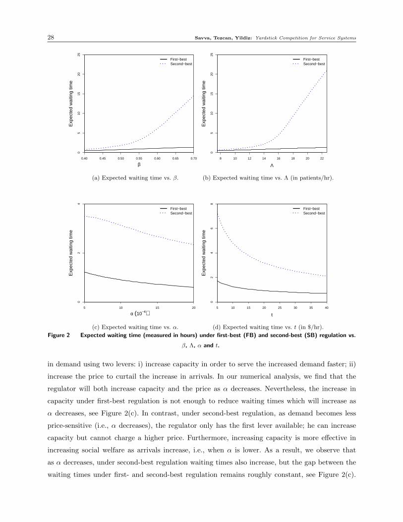
28 Savva, Tezcan, Yildiz: Yardstick Competition for Service Systems
0.40 0.45 0.50 0.55 0.60 0.65 0.70
05
1015
2025
First−bestSecond−best
β
Exp
ecte
d w
aitin
g tim
e
(a) Expected waiting time vs. β.
8 10 12 14 16 18 20 22
05
1015
2025
First−bestSecond−best
Λ
Exp
ecte
d w
aitin
g tim
e
(b) Expected waiting time vs. Λ (in patients/hr).
First−bestSecond−best
5 10 15 20
02
4
α (10−4)
Exp
ecte
d w
aitin
g tim
e
(c) Expected waiting time vs. α.
5 10 15 20 25 30 35 40
02
46
8First−bestSecond−best
t
Exp
ecte
d w
aitin
g tim
e
(d) Expected waiting time vs. t (in $/hr).
Figure 2 Expected waiting time (measured in hours) under first-best (FB) and second-best (SB) regulation vs.
β, Λ, α and t.
in demand using two levers: i) increase capacity in order to serve the increased demand faster; ii)
increase the price to curtail the increase in arrivals. In our numerical analysis, we find that the
regulator will both increase capacity and the price as α decreases. Nevertheless, the increase in
capacity under first-best regulation is not enough to reduce waiting times which will increase as
α decreases, see Figure 2(c). In contrast, under second-best regulation, as demand becomes less
price-sensitive (i.e., α decreases), the regulator only has the first lever available; he can increase
capacity but cannot charge a higher price. Furthermore, increasing capacity is more effective in
increasing social welfare as arrivals increase, i.e., when α is lower. As a result, we observe that
as α decreases, under second-best regulation waiting times also increase, but the gap between the
waiting times under first- and second-best regulation remains roughly constant, see Figure 2(c).

Savva, Tezcan, Yildiz: Yardstick Competition for Service Systems 29
Naturally, since the gap in waiting times remains constant as α increases while the total welfare
decreases as demand becomes more price-sensitive (i.e., α increases), the welfare loss associated
with second-best compared to first-best regulation also increases in α, as observed in Figure 1.
We next examine the impact of the cost of waiting t on the welfare ratio. We note that it
has a less pronounced impact on the welfare ratio than the other parameters (β, Λ, or α), as
shown in Figure 1. To see why this is the case, note that if t is high, then under either first-
or second-best regulation, the system operates at relatively low utilization, resulting in relatively
low waiting times, see Figure 2(d). Hence, the over-joining behaviour observed under second-best
regulation does not affect social welfare as much. If, on the other hand, t is low, under either type of
regulation, the system will operate under high utilization, resulting in long waiting times, see again
Figure 2(d). However, since the waiting time cost t is low, customers are less sensitive to delays
and therefore social welfare is, again, not greatly affected by the inefficient over-joining behaviour
under second-best regulation.
6.3. Impact of misestimating the cost of waiting
To implement the proposed payment schemes, the regulator needs to estimate the cost of waiting,
t. We next test the impact of potential estimation errors on total social welfare using the following
procedure. We assume that t= $20 and that the regulator misestimates this cost and sets it equal to
to( 6= t) in (16)-(17) for first-best and in (23) for second-best regulation. We identify the equilibrium
for each to ranging from $0.1 to $40 in increments of $0.1 by solving the first-order conditions of
the provider’s objective and verifying that the provider’s objective is maximised with these actions.
We then compare the welfare in this equilibrium to the base case, i.e., when the regulator estimates
t accurately. We present the welfare ratio as a function of to in Figures 3(a) and 3(b) for first-
and second-best regulation, respectively. Under second-best regulation the providers exert no effort
in capacity expansion in equilibrium for to ≤ $4.57 hence we plot the welfare ratio beyond this
point only. In addition, again for second-best regulation, there exist two symmetric equilibria for
$4.57≤ to ≤ $5.10 and so we only report the welfare ratio using the equilibrium that results in a
lower welfare loss.
It is clear from from Figure 3 that estimation error in the cost of waiting t generates a loss of
welfare. When t is underestimated, providers operate under high utilisation simply because they
are not incentivized enough to cut wait times. When t is overestimated, the providers invest more
in costly capacity which is underutilized. Nevertheless, there are two interesting observations. First,
the welfare loss under first-best regulation is less sensitive to estimation errors than under second-
best. Second, the impact of the estimation error is more substantial when t is underestimated (it
reaches 70% and 54% in first- and second-best, respectively) compared to when it is overestimated

30 Savva, Tezcan, Yildiz: Yardstick Competition for Service Systems
0 10 20 30 400 10 20 30 40
0.6
0.7
0.8
0.9
1
to
Wel
fare
Rat
io
(a) First-best regulation.
0 10 20 30 400 10 20 30 40
0.4
0.5
0.6
0.7
0.8
0.9
1
µo* = µo
4.57
to
Wel
fare
Rat
io
(b) Second-best regulation.
Figure 3 Ratio of realized to first-best (second-best) welfare vs. miss-estimated cost of waiting to. Actual cost
of waiting is = $20. Other parameters set to base case.
(it is above 99.8% and 98% in first- and second-best, respectively, when to ≥ t).7 We believe that
this has to do with the fact that waiting times are convex in capacity – starting from the optimal
capacity (set when t is estimated accurately), a small decrease in capacity (due to t being under-
estimated), will generate a greater loss of welfare due to a larger increase in waiting times than
the welfare gain associated with the small reduction in waiting-times generated by a small increase
in capacity (due to t being overestimated). Hence, the welfare loss is more substantial when t is
underestimated than it is overestimated.
The fact that total welfare is not very sensitive to the actual cost-of-waiting assumed by the
regulator points to the fact that social welfare is relatively flat around the the actual cost t. An
overestimate in the cost of waiting will generate a welfare loss due to installing more capacity
than optimal that will be almost fully compensated by an increase in welfare due to the associated
reduction in waiting times and increase in demand. In light of the discussion above, the regulator
may be able to use the waiting-time cost parameter t as a lever to influence waiting times; by
choosing to implement a regulatory scheme with high t, the regulator shifts the equilibrium outcome
towards lower waiting times, at the expense of higher hospital costs, without sacrificing much in
terms of total welfare.
7 We verify the robustness of this observation by generating 1000 random scenarios for Λ, α, and β using the rangesspecified in Table 1. In all scenarios, we set t= $20. As in the case above, we find the welfare loss under first- andsecond-best regulation if the regulator first underestimates t to to = $10 and second, overestimates t to t0 = $30. Inall the parameter combinations the welfare loss for first-best regulation was minimal; the average welfare loss wasequal to 0.2%, with maximum loss equal to 0.3% for to = $10 and it was equal to 0.05% with maximum loss equal to0.1%, for t0 = $30. In the second-best (excluding three scenarios which did not have an equilibrium) for to = $10, theaverage welfare loss was equal to 3.53% with maximum loss equal to 40.2% and for to = $30, the average welfare losswas 0.4% with maximum loss equal to 3.6%. In addition, the welfare loss was lower for to = $30 than for to = $10 inall the scenarios under both first- and second-best regulation.

Savva, Tezcan, Yildiz: Yardstick Competition for Service Systems 31
7. Conclusions
This paper investigates the use of yardstick competition, a regulatory scheme that creates cost-
reduction incentives (Shleifer 1985), in service settings where, in addition to cost control, the
regulator is also interested in incentivizing wait-time reduction. This scheme has proliferated in
the regulation (and reimbursement) of hospitals (Fetter 1991). We find that the standard form
of yardstick competition fails in this second dimension of performance. Perhaps this finding helps
explain the persistently long waiting times experienced by patients in many healthcare systems
throughout the world.
We also present two alternative schemes that fare better. The first scheme, which involves a
provider-specific customer fee, achieves first-best investment in both cost and wait-time reduction,
but is rather difficult to implement in practice – besides the customer fee being politically sensitive
in healthcare setting, this scheme places a high informational burden on the regulator with respect
to the queueing discipline. The second scheme, which assumes that the service is funded exclusively
through transfer payments (e.g., taxes or insurance premia), may be easier to implement. In essence,
this scheme modifies the transfer payment of the standard cost-based yardstick competition by
adding a component which is decreasing in the difference between the average waiting times of
each provider and that of an exogenous benchmark constructed by averaging the waiting time of all
other providers. We also show how this scheme can be implemented in a relatively straightforward
way in systems with multiple customer classes, time-varying arrival rates, more complex cost
structures, and heterogeneous providers. The simplicity of this second regulatory scheme comes
at a cost of efficiency as it no longer achieves first-best incentives. Nevertheless, as our numerical
investigation illustrates, it is likely to be better than the status quo where waiting-time reduction
is not incentivized.
We hope that this paper will contribute to the current debate on how to best incentivize invest-
ment in waiting-time reduction in healthcare, particularly in Emergency Departments where wait-
ing times have been argued to be undesirably long. In fact, our paper provides a high-level guideline
for regulators, such as CMS in the US and the NHS in the UK who have started monitoring ED
waiting times, on how to use waiting-time information in the reimbursement formula. We believe
that this is a promising alternative to top-down targets, such as the four-hour target that has been
implemented in the UK for patients visiting EDs (see, e.g., Campbell (2016)).
Of course, the exact application may be complicated, especially by concerns about patient selec-
tion based on service times or system congestion. We believe this may not be a problem in practice,
as was the case with the advent of cost-based yardstick competition which is not believed to have
given rise to significant selection based on costs. Nevertheless, understanding and mitigating selec-
tion problems that arise in the presence of waiting-time yardstick competition is an issue that
32 Savva, Tezcan, Yildiz: Yardstick Competition for Service Systems
future research should address. An additional limitation of this work is that all of the schemes
proposed assume that the regulator knows the cost of customer waiting per unit time, t. This may
not always be the case, but, as we show in our numerical investigation, total welfare is not sensitive
to the precise value that it takes. In fact, one may view the waiting-time cost parameter t as a lever
that can be used to influence waiting times; by choosing to implement a regulatory scheme with
high t, the regulator shifts the equilibrium outcome towards lower waiting times at the expense
of higher costs with little loss in overall welfare. Nevertheless, identifying a modified scheme that
does not require this information may be a promising direction for further research. Finally, we
note that our analysis assumes that the service providers are regional monopolists, i.e., they do
not compete directly for customers. While the presence of direct competition would make the need
for regulatory intervention less pronounced, it would nevertheless be of interest to examine the
performance of the proposed scheme under (imperfect) competition.
References
Adida, E., H. Mamani, S. Nassiri. 2016. Bundled payment vs. fee-for-service: Impact of payment scheme on
performance. Management Science Forthcoming.
Afeche, P. 2013. Incentive-compatible revenue management in queueing systems: Optimal strategic delay.
Manufacturing & Service Operations Management 15(3) 423–443.
Akan, M., B. Ata, M. A. Lariviere. 2011. Asymmetric information and economies of scale in service con-
tracting. Manufacturing & Service Operations Management 13(1) 58–72.
Allon, G., A. Federgruen. 2007. Competition in service industries. Operations Research 55(1) 37–55.
Allon, G., A. Federgruen. 2008. Service competition with general queueing facilities. Operations Research
56(4) 827–849.
Anand, K. S., M. F. Pac, S. Veeraraghavan. 2011. Quality-speed conundrum: Trade-offs in customer-intensive
services. Management Science 57(1) 40–56.
Andritsos, D. A., S. Aflaki. 2015. Competition and the operational performance of hospitals: The role of
hospital objectives. Production and Operations Management 24(11) 1812–1832.
Andritsos, D. A., C. S. Tang. 2015. Incentive programs for reducing readmissions when patient care is
co-produced. Working Paper No. MOSI-2015-1110, HEC Paris, Paris, France.
Armony, M., S. Israelit, A. Mandelbaum, Y. N. Marmor, Y. Tseytlin, G. B. Yom-Tov. 2015. Patient flow in
hospitals: A data-based queueing-science perspective. Stochastic Systems 5(1) 146–194.
Armstrong, M., R. H. Porter. 2007. Handbook of Industrial Organization Vol. 3 . Elsevier, Amsterdam,
Netherlands.
Bakshi, N., S. H. Kim, N. Savva. 2015. Signaling new product reliability with after-sales service contracts.
Management Science 61(8) 1812–1829.

Savva, Tezcan, Yildiz: Yardstick Competition for Service Systems 33
Batt, R. J., C. Terwiesch. 2015. Waiting patiently: An empirical study of queue abandonment in an emergency
department. Management Science 61(1) 39–59.
Besley, T., A. Case. 1995. Incumbent behavior: Vote seeking, tax setting and yardstick competition. American
Economic Review 85(1) 25–45.
Bordignon, M., F. Cerniglia, F. Revelli. 2003. In search of yardstick competition: a spatial analysis of Italian
municipality property tax setting. Journal of Urban Economics 54(2) 199–217.
Brown, A. M., S. L. Decker, F. W. Selck. 2015. Emergency department visits and proximity to patients’
residences, 2009-2010. NCHS Data Brief (192) 1–8.
Bureau of Labor Statistics. 2011. Occupational Employment Statistics. Accessed December 11, 2016, http:
//www.bls.gov/oes/oes_perc.htm.
Cachon, G., P. T. Harker. 2002. Competition and outsourcing with scale economies. Management Science
48(10) 1314–1333.
Cachon, G. P., F. Zhang. 2006. Procuring fast delivery: Sole sourcing with information asymmetry. Man-
agement Science 52(6) 881–896.
Campbell, D. 2016. NHS trust bosses slam £600m hospital fines over patient targets.
The Guardian (March 29), https://www.theguardian.com/society/2016/mar/29/
nhs-bosses-slam-600m-hospital-fines-over-patient-targets.
Campbell, D., R. Mason. 2013. A&E overcrowding may cost lives, emergency doctors
warn. The Guardian (November 5), http://www.theguardian.com/society/2013/nov/06/
accident-emergency-overcrowding-costs-lives-doctors.
Canadian Institute for Health Information. 2012. Canadians continue to wait for care. Accessed Decem-
ber 11, 2016, https://www.cihi.ca/en/health-system-performance/access-and-wait-times/
canadians-continue-to-wait-for-care.
CEB. 2016. 2016 Medical plan trends and observations report. Accessed December 11, 2016, https://www.
cebglobal.com/human-resources/total-rewards/medical-plan-trends.html.
CMS. 2011. National hospital ambulatory medical care survey: 2011 emergency department summary tables.
Accessed December 11, 2016, http://www.cdc.gov/nchs/data/ahcd/nhamcs_emergency/2011_ed_
web_tables.pdf.
CMS. 2014. Financial report fiscal year 2014. Accessed December 11, 2016, https://www.cms.
gov/Research-Statistics-Data-and-Systems/Statistics-Trends-and-Reports/CFOReport/
Downloads/CMS-Financial-Report-for-Fiscal-Year-2014.pdf.
CMS. 2016a. Hospital value-based purchasing. Accessed December 11, 2016, https://www.cms.gov/
Outreach-and-Education/Medicare-Learning-Network-MLN/MLNProducts/downloads/Hospital_
VBPurchasing_Fact_Sheet_ICN907664.pdf.

34 Savva, Tezcan, Yildiz: Yardstick Competition for Service Systems
CMS. 2016b. Hospital Compare: Find a hospital. Accessed December 11, 2016, https://www.medicare.
gov/hospitalcompare/search.html.
Dalen, D. M. 1998. Yardstick competition and investment incentives. Journal of Economics & Management
Strategy 7(1) 105–126.
Deo, S., I. Gurvich. 2011. Centralized vs. decentralized ambulance diversion: A network perspective. Man-
agement Science 57(7) 1300–1319.
Do, H., M. Shunko. 2016. Pareto improving coordination policies in queueing systems: Application to
flow control in emergency medical services. Working paper, Krannert School of Management, Purdue
University, West Lafayette, IN.
Dranove, D. 1995. Measuring costs. Frank A. Sloan, ed., Valuing health care: Costs, Benefits, and Effec-
tiveness of Pharmaceuticals and Other Medical Technologies. Cambridge University Press, Cambridge,
UK. 61–76.
Edelson, N. M., D. K. Hilderbrand. 1975. Congestion tolls for Poisson queuing processes. Econometrica
43(1) 81–92.
Ellis, R. P., T. G. McGuire. 1986. Provider behavior under prospective reimbursement: Cost sharing and
supply. Journal of Health Economics 5(2) 129–151.
Fetter, R. B. 1991. Diagnosis related groups: Understanding hospital performance. Interfaces 21(1) 6–26.
Freeman, M., N. Savva, S. Scholtes. 2016. Economies of scale and scope in hospitals. Working paper, Judge
Business School, University of Cambridge, Cambridge, UK.
Gans, N., G. Koole, A. Mandelbaum. 2003. Telephone call centers: Tutorial, review, and research prospects.
Manufacturing & Service Operations Management 5(2) 79–141.
Gaynor, M. 2004. Competition and quality in hospital markets. What do we know? What don’t we know?
Economie Publique, 15(2) 3–40.
Gilboy, N., T. Tanabe, D. Travers, A. M. Rosenau. 2011. Emergency severity index (ESI): A triage tool
for emergency department care version 4. Tech. Rep. AHRQ Publication No. 12-0014, Agency for
Healthcare Research and Quality, Rockville, MD.
Government Accountability Office. 2009. Hospital emergency departments: Crowding continues to occur,
and some patients wait longer than recommended time frames. Accessed December 11, 2016, http:
//www.gao.gov/new.items/d09347.pdf.
Grannemann, T. W., R. S. Brown, M. V. Pauly. 1986. Estimating hospital costs: A multiple-output analysis.
Journal of Health Economics 5(2) 107–127.
Guo, P., C. S. Tang, Y. Wang, M. Zhao. 2016. The impact of reimbursement policy on patient welfare,
readmission rate and waiting time in a public healthcare system: Fee-for-service vs. bundled payment.
Working paper, Anderson School of Management, University of California, Los Angeles, CA.

Savva, Tezcan, Yildiz: Yardstick Competition for Service Systems 35
Hasija, S., E. J. Pinker, R. A. Shumsky. 2008. Call center outsourcing contracts under information asymmetry.
Management Science 54(4) 793–807.
Hassin, R. 2016. Rational Queueing . CRC Press, Boca Raton, FL.
Hassin, R., M. Haviv. 2003. To Queue or Not to Queue: Equilibrium Behavior in Queueing Systems. Kluwer
Academic Publishers, Norwell, MA.
Holmstrom, B. 1982. Moral hazard in teams. The Bell Journal of Economics 13(2) 324–340.
Jamasb, T., M. Pollitt. 2000. Benchmarking and regulation: International electricity experience. Utilities
Policy 9(3) 107–130.
Jiang, H., Z. Pang, S. Savin. 2012. Performance-based contracts for outpatient medical services. Manufac-
turing & Service Operations Management 14(4) 654–669.
Jiang, H., Z. Pang, S. Savin. 2016. Capacity management for outpatient medical services under competi-
tion and performance-based incentives. Working paper, Wharton School, University of Pennsylvania,
Philadelphia, PA.
Kim, S. H., M. A. Cohen, S. Netessine. 2007. Performance contracting in after-sales service supply chains.
Management Science 53(12) 1843–1858.
Kim, S. H., M. A. Cohen, S. Netessine, S. Veeraraghavan. 2010. Contracting for infrequent restoration and
recovery of mission-critical systems. Management Science 56(9) 1551–1567.
Kleinrock, L. 1975. Queueing Systems, Volume I: Theory . John Wiley & Sons Inc., New York, NY.
Laffont, J. J., J. Tirole. 1993. A Theory of Incentives in Procurement and Regulation. MIT Press, Cambridge,
MA.
Lariviere, M. A., J. A. Van Mieghem. 2004. Strategically seeking service: How competition can generate
poisson arrivals. Manufacturing & Service Operations Management 6(1) 23–40.
Lee, D. K. K., S. A. Zenios. 2012. An evidence-based incentive system for Medicare’s End-Stage Renal
Disease program. Management Science 58(6) 1092–1105.
Lee, H. L., M. A. Cohen. 1985. Multi-agent customer allocation in a stochastic service system. Management
Science 31(6) 752–763.
Lefouili, Y. 2015. Does competition spur innovation? The case of yardstick competition. Economics Letters
137 135–139.
Ma, C. A. 1994. Health care payment systems: Cost and quality incentives. Journal of Economics &
Management Strategy 3(1) 93–112.
Mayes, R. 2007. The origins, development, and passage of Medicare’s revolutionary prospective payment
system. Journal of the History of Medicine and Allied Sciences 62(1) 21–55.
McHugh, M., P. Tanabe, M. McClelland, R. K. Khare. 2012. More patients are triaged using the Emergency
Severity Index than any other triage acuity system in the United States. Academic Emergency Medicine
19(1) 106–109.

36 Savva, Tezcan, Yildiz: Yardstick Competition for Service Systems
Mendelson, H., S. Whang. 1990. Optimal incentive-compatible priority pricing for the M/M/1 queue. Oper-
ations research 38(5) 870–883.
Meran, G., C. Von Hirschhausen. 2009. A modified yardstick competition mechanism. Journal of Regulatory
Economics 35(3) 223–245.
Nalebuff, B. J., J. E. Stiglitz. 1983. Information, competition, and markets. The American Economic Review
73(2) 278–283.
Naor, P. 1969. The regulation of queue size by levying tolls. Econometrica 37(1) 15–24.
Pope, G. C. 1989. Hospital nonprice competition and Medicare reimbursement policy. Journal of Health
Economics 8(2) 147–172.
Rajan, B., A. Seidmann, T. Tezcan. 2014. Service systems with heterogeneous customers: Investigating the
effect of telemedicine on patient care. Tech. rep., University of Rochester.
Ren, Z. J., Y. P. Zhou. 2008. Call center outsourcing: Coordinating staffing level and service quality.
Management Science 54(2) 369–383.
Ringel, J. S., S. D. Hosek, B. A. Vollaard, S. Mahnovski. 2002. The elasticity of demand for health care. A
review of the literature and its application to the military health system. Tech. rep., National Defense
Research Institute, RAND Health, Santa Monica, CA.
Roques, F. A., N. Savva. 2009. Investment under uncertainty with price ceilings in oligopolies. Journal of
Economic Dynamics and Control 33(2) 507–524.
Saghafian, S., G. Austin, S. J. Traub. 2015. Operations research/management contribu-
tions to emergency department patient flow optimization: Review and research prospects.
IIE Transactions on Healthcare Systems Engineering 5(2) 101–123.
Saghafian, S., W. J. Hopp, M. P. Van Oyen, J. S. Desmond, S. L Kronick. 2014. Complexity-augmented triage:
A tool for improving patient safety and operational efficiency. Manufacturing & Service Operations
Management 16(3) 329–345.
Sawkins, J. W. 1995. Yardstick competition in the English and Welsh water industry Fiction or reality?
Utilities Policy 5(1) 27–36.
Shleifer, A. 1985. A theory of yardstick competition. The RAND Journal of Economics 16(3) 319–327.
Siddique, H. 2016. Hospital A&E waiting times in england rise by a third in Novem-
ber. The Guardian (January 14), https://www.theguardian.com/society/2016/jan/14/
hospital-waiting-times-england-rise-november-accident-emergency.
So, K. C., C. S. Tang. 2000. Modeling the impact of an outcome-oriented reimbursement policy on clinic,
patients, and pharmaceutical firms. Management Science 46(7) 875–892.
Sobel, J. 1999. A reexamination of yardstick competition. Journal of Economics & Management Strategy
8(1) 33–60.

Savva, Tezcan, Yildiz: Yardstick Competition for Service Systems 37
Stidham, S. Jr. 2009. Optimal Design of Queueing Systems. CRC Press, Boca Raton, FL.
Tanger̊as, T. P. 2009. Yardstick competition and quality. Journal of Economics & Management Strategy
18(2) 589–613.
Thomson, R. B. 1994. Competition among hospitals in the United States. Health Policy 27(3) 205–231.
Wang, G., J. Li, W. J. Hopp, F. L. Fazzalari, S. Bolling. 2016. Using patient-centric quality information to
unlock hidden health care capabilities. Working Paper No. 1291, Ross School of Business, University
of Michigan, Ann Arbor, MI.
Weitzman, M. L. 1978. Optimal rewards for economic regulation. The American Economic Review 68(4)
683–691.
Williams, B., J. Nicholl, J. Brazier. 2004. Accident and emergency departments. A. Stevens, J. Raftery,
eds., Health Care Needs Assessment: The Epidemiologically Based Needs Assessment Reviews. Radcliffe
Medical Press, Oxford, UK. 1-54.
Williams, R. M. 1996. Distribution of emergency department costs. Annals of Emergency Medicine 28(6)
671–676.
Zhang, D. J., I. Gurvich, J. A. Van Mieghem, E. Park, R. S. Young, M. V. Williams. 2016. Hospital readmis-
sions reduction program: An economic and operational analysis. Management Science Forthcoming.

38 Savva, Tezcan, Yildiz: Yardstick Competition for Service Systems
Appendix
A. Conditions
As is often the case in queueing games, we have made the assumption that first order conditions
(FOC) are necessary and sufficient for both the regulator’s and the individual provider’s problems
(see for example Mendelson and Whang (1990)). This assumption however may not always hold
(Stidham 2009). For this reason, in this section, we present additional conditions which ensure
that FOC are sufficient for the specific case of the M/M/1 queue. More specifically, we provide
sufficient (but not necessary) conditions for
• FOC to be necessary and sufficient for determining the first- and second-best solutions of the
regulator’s welfare maximization problem of Propositions 1 and 4 (see Appendices A.1 and A.4,
respectively).
• FOC to be necessary and sufficient for the provider’s profit maximization problem under
the payment schemes of Propositions 2, Theorems 1 and 2 (see Appendices A.2, A.3, and A.5,
respectively).
Where applicable, we compare the conditions presented here to the closest extant literature (Shleifer
1985). We note that these conditions can all be interpreted as either assumptions about the cost
function R(c,µ), which, loosely speaking, needs to be “sufficiently” convex for the objective func-
tions to be well-behaved, or about the default capacity µ0 (and default cost c0), which needs to
be sufficiently small (large) to allow for interior solutions. We also note that these conditions are
sufficient but by no means necessary.
A.1. Assumptions for Proposition 1: Regulator’s First-Best Solution
We present sufficient conditions for the FOC to be necessary and sufficient to obtain the regulators’
optimal (first-best) actions. We begin by defining λ∗(c,µ)∈ [0,Λ] by
Θ̄−1
(λ∗(c,µ)
Λ
)=
tµ
(µ−λ∗(c,µ))2+ c, (30)
and µ∗(c)≥ µo by
tλ∗(c,µ∗(c))
(µ∗(c)−λ∗(c,µ∗(c))2=
∂
∂µR(c,µ∗(c)) (31)
for c∈ (0, co] and µ≥ µo. We show that λ∗(c,µ) and µ∗(c) are well-defined in the proof of Proposition
5 below. We next define Conditions 1–5 that are used in the next proposition.
Condition 1: tλ∗(c,µ)
(µ−λ∗(c,µ))2is decreasing in µ for µ≥ µ0 and c∈ (0, co],
Condition 2: tλ∗(c,µo)
(µo−λ∗(c,µo))2− ∂R(c,µo)
∂µ> 0 for c∈ (0, co],
Condition 3:(−λ∗(c,µ∗(c))− dR(c,µ∗(c))
dc
)is decreasing in c for c∈ (0, co],
Condition 4: λ∗(0, µ∗(0))<−(∂R(0,µ∗(0))
∂c+ ∂R(0,µ∗(0))
∂µ
),
Condition 5: λ∗(co, µ∗(co))>−
(∂R(co,µ
∗(co))
∂c+ ∂R(co,µ
∗(co))
∂µ
).

Savva, Tezcan, Yildiz: Yardstick Competition for Service Systems 39
Proposition 5. Conditions 1–5 are sufficient for the FOC to be necessary and sufficient for
the regulator’s welfare maximization problem to define the first-best solution.
Conditions 2, 4 and 5 are the boundary conditions that guarantee that first-best outcomes are
interior. Condition 1 ensures the concavity of welfare function in capacity µ for all c∈ (0, co] when
customers join at rate λ∗(c,µ). Condition 3 is a necessary and sufficient condition for the concavity
of welfare function in cost per customer c when customers join at rate λ∗(c,µ) and the provider
chooses capacity level µ∗(c).
Conditions 3–5 are similar to the conditions in Shleifer (1985) (given in (44) and (45)) that
guarantee that FOC are sufficient if waiting time is not costly. The only difference is that Shleifer
(1985) inherently assumes that capacity is fixed at its default level, µo, and hence defines conditions
for capacity level µo instead of µ∗(c).
Proof of Proposition 5: We proceed in three main steps.
Step i) First we show that for fixed c ∈ [0, co] and µ ∈ [µo,∞) there exists a unique p ≥ 0,
denoted by p∗(c,µ), that maximizes S(p, c,µ), that is,
S(p∗(c,µ), c, µ) = maxp≥0
S(p, c,µ).
Step ii) Then we show that for fixed c ∈ [0, co], µ∗(c) defined in (31) is unique and maximizes
S(p∗(c,µ), c, µ), that is,
S(p∗(c,µ∗(c)), c, µ∗(c)) = max0≤µ≤co
S(p(c,µ), c, µ).
Step iii) Next we show that there exists a unique c∗ ∈ (0, co) that maximizes
S(p∗(c,µ∗(c)), c, µ∗(c)), that is,
S(p∗(c,µ∗(c∗)), c∗, µ∗(c∗)) = max0≤c≤co
S(p(c,µ), c, µ∗(c)).
We provide the details of these steps next.
Step i) To prove the existence and uniqueness of p∗(c,µ) we show that S(p, c,µ) is a concave
function of p and p∗(c,µ) is not at the boundaries, i.e. p∗(c,µ) ∈ (0,∞), for fixed c ∈ [0, co] and
µ∈ [µo,∞). By Leibnitz rule
∂
∂y
(Λ
∫ ∞Θ̄−1( yΛ)
xdΘ(x)
)=−ΛΘ̄−1
( yΛ
)θ(
Θ̄−1( y
Λ
)) ∂Θ̄−1(yΛ
)∂y
= Θ̄−1( y
Λ
)for y ∈ [0,Λ]. (32)
By (6) we have
∂
∂pS(p, c,µ) = f(p, c,µ)
∂
∂pλ(p,µ), (33)

40 Savva, Tezcan, Yildiz: Yardstick Competition for Service Systems
where, by (32), f is given by
f(p, c,µ) := Θ̄−1
(λ(p,µ)
Λ
)− tµ
(µ−λ(p,µ))2− c. (34)
Let v : [0,Λ]→ [0,∞) be defined by
v(λ) = Θ̄−1(λ/Λ). (35)
By (2) we have
∂
∂pλ(p,µ)< 0, for p≥ 0 and µ≥ µo. (36)
Therefore, to show S(p, c,µ) is concave in p it is enough to show that f(p, c,µ) is increasing in p.
By (34)
∂
∂pf(p, c,µ) =
(ν ′(λ(p,µ))− 2tµ
(µ−λ(p,µ))3
)∂
∂pλ(p,µ). (37)
(We use ′ to denote the derivative of functions whose domain is one dimensional) We have ν ′(y)< 0
for all y ∈ [0,Λ] because θ(x)≥ 0 for x≥ 0, and that λ(p,µ)<µ by (2). Hence f(p, c,µ) is increasing
in p.
To show that p∗(c,µ) > 0 and is unique we next show that ∂∂pS(0, c, µ) > 0 and
limp→∞∂∂pS(p, c,µ)< 0. By (34)
f(0, c, µ) = ν (λ(0, µ))− tµ
(µ−λ(0, µ))2− c=
t
µ−λ(0, µ)− tµ
(µ−λ(0, µ))2− c < 0, (38)
where the second equality follows from (2), giving ∂∂pS(0, c, µ)> 0. Also, since limp→∞ λ(p,µ) = 0
for all µ≥ µo by (2), we have
limp→∞
f(p, c,µ)> 0, (39)
giving limp→∞∂∂pS(p, c,µ)< 0.
Therefore, for any c ∈ [0, co] and µ ∈ [µo,∞), there exists a unique optimal p∗(c,µ) ∈ (0,∞),
which is obtained by
∂
∂pS(p∗(c,µ), c, µ) = ν (λ(p∗(c,µ), µ))− tµ
(µ−λ(p∗(c,µ), µ))2− c= 0. (40)
This also proves the existence and uniqueness of λ∗(c,µ) defined in (30).
Step ii) To prove that there exists a unique µ∈ (µo,∞) that maximizes S(p∗(c,µ), c, µ) for fixed
0≤ c≤ co, we show that (i) S(p∗(c,µ), c, µ) is concave in µ. (ii) limµ↓µoddµS(p∗(c,µ), c, µ)> 0 and
(iii) limµ→∞ddµS(p∗(c,µ), c, µ)< 0. By (6) and (32),
d
dµS(p∗(c,µ), c, µ) =
(ν(λ∗(c,µ))− tµ
(µ−λ∗(c,µ))2− c)∂
∂µλ∗(c,µ) +
tλ∗(c,µ)
(µ−λ∗(c,µ))2− ∂R(c,µ)
∂µ

Savva, Tezcan, Yildiz: Yardstick Competition for Service Systems 41
=tλ∗(c,µ)
(µ−λ∗(c,µ))2− ∂R(c,µ)
∂µ, (41)
where (41) follows from (40). By Condition 1 and that ∂R(c,µ)
∂µis increasing in µ by convexity of
R, ddµS(p∗(c,µ), c, µ) is decreasing; and hence, S(p∗(c,µ), c, µ) is concave in µ. By Condition 2 and
(41), we have ddµS(p∗(c,µo), c, µo)> 0. Also, by (41), convexity of R and λ∗(c,µ)≤Λ by (2), we get
limµ→∞
d
dµS(p∗(c,µ), c, µ) = lim
µ→∞−∂R(c,µ)
∂µ< 0. (42)
Thus, the optimal capacity µ∗(c) given any c∈ (0, co] can be obtained by (31).
Step iii) Finally, we show that there is a unique c∈ (0, co) that maximizes S(p∗(c,µ∗(c)), c, µ∗(c)).
Let S∗(c) = S(p∗(c,µ∗(c)), c, µ∗(c)) for notational simplicity. By (6) and (32), we have
∂S∗(c)
∂c=
(ν(λ∗(c,µ∗(c)))− tµ∗(c)
(µ∗(c)−λ∗(c,µ∗(c)))2− c)d
dcλ∗(c,µ∗(c))
+
(tλ∗(c,µ∗(c))
(µ∗(c)−λ∗(c,µ∗(c)))2− ∂R(c,µ∗(c))
∂µ
)∂µ∗(c)
∂c−λ∗(c,µ∗(c))− dR(c,µ∗(c))
dc
=−λ∗(c,µ∗(c))− dR(c,µ∗(c))
dc, (43)
where (43) follows from (30) and (31). By (43) and Condition 3, dS∗(c)dc
is decreasing and hence
S∗(c) is strictly concave in c. In addition, by Conditions 4 and 5, we have dS∗(0)
dc> 0 and dS∗(co)
dc< 0.
Thus, there exists a unique global maximum c∗ of S∗(c) and (p∗(c∗, µ∗(c∗)), µ∗(c∗), c∗) is the unique
optimizer of S(c, p,µ) and satisfies the FOC (10)–(12). Because (40), (41) and (43) have unique
solutions, (p∗(c∗, µ∗(c∗)), µ∗(c∗), c∗) is the unique point that satisfies the FOC. �
A.2. Assumptions for Proposition 2
We provide sufficient conditions that guarantee the FOCs of the provider’s profit maximization
problem to be necessary and sufficient under the payment scheme of Proposition 2. Since this is
the problem studied in Shleifer (1985), these conditions were first presented in Shleifer (1985).
Expressed in our notation, these are that R(c,µo) is convex in c and
∂λ(c,µo)
∂c+∂2R(c,µo)
∂c2> 0, (44)
along with the boundary conditions
λ(co, µo) +∂
∂cR(co, µo)> 0 and λ(0, µo) +
∂
∂cR(0, µo)< 0. (45)
Further to Shleifer (1985), we need to also assume that (44) holds for all µ≥ µ0. These conditions
ensure that the objective function of the provider is concave and the solution is interior for all
µ≥ µ0.

42 Savva, Tezcan, Yildiz: Yardstick Competition for Service Systems
A.3. Assumptions for Theorem 1
We provide sufficient conditions that guarantee the FOCs of the provider’s profit maximization
problem to be necessary and sufficient under the payment scheme of Theorem 1. The provider’s
profit is given by (18) and if R is strictly convex then Π is strictly concave. If in addition the optimal
actions for the provider are not at the boundaries, then the FOC are necessary and sufficient to
determine the provider’s optimal actions. We next present sufficient conditions that guarantee that
the maximum is attained at an interior point.
The following conditions imply that c∗ ∈ (0, co).
∂
∂cR(co, µ)>−λ(co, µo) and
∂
∂cR(0, µ)<−Λ, for all µ≥ µo. (46)
This follows from (18) because R is convex in c and λ̄i ∈ [λ(co, µo),Λ] for all i.
To list conditions that are sufficient for µ∗ ∈ (µo,∞) we first introduce some terminology. By (2)
and (16) t(µ̄i−λ̄i)
≤ v(λmin) for all i= 1, . . . ,N . Hence there exists K > 0 such that
λ̄it
(µ̄i− λ̄i)2<K.
In addition this implies that it is never optimal to set µ≥M in any equilibrium for a provider by
(18) for some M > 0. The following conditions are sufficient for µ∗ to be an interior point. Assume
that there exits µK such that ∂∂µR(c,µ)>K for µ≥ µK and for any c∈ [0, co] and that
∂
∂µR(c,µo)<
tλ(co, µo)
(M −λ(co, µo))2 , for all c∈ [0, co]. (47)
The fact that µ∗ ∈ (µo,∞) follows from these conditions because; i) R is convex in µ, ii) tλ
(µ−λ(c,µ))2
is minimized at µ= µo and c= co and (iii) M is an upper bound for µ.
A.4. Assumptions for Proposition 4: Regulator’s Second-Best Solution
We present sufficient conditions for the FOC to be necessary and sufficient to obtain the regulators’
optimal (second-best) actions.
Let c̃(µ) be the solution of
∂
∂cR(c̃(µ), µ) =−λ(µ) for µ≥ µo. (48)
We show that c̃(µ) is well-defined in the proof of Proposition 6 below. We first define Conditions
6–9 that are used in the next proposition.
Condition 6: λ(µ)<−∂R(0,µ)
∂cfor µ≥ µo,
Condition 7: λ(µ)>−∂R(co,µ)
∂cfor µ≥ µo,
Condition 8:(
tλ(µ)
(µ−λ(µ))2
(1− ∂λ(µ)
∂µ
)− c̃(µ)∂λ(µ)
∂µ− d
dµR(c̃(µ), µ)
)is decreasing for µ≥ µo,
Condition 9:(
tλ(µo)
(µo−λ(µo))2
(1− ∂λ(µo)
∂µ
)− c̃(µo)∂λ(µo)
∂µ
)> ∂
∂cR(c̃(µo), µo) + ∂
∂µR(c̃(µo), µo).

Savva, Tezcan, Yildiz: Yardstick Competition for Service Systems 43
Proposition 6. Conditions 6–9 are sufficient for the FOC of the regulator’s problem to be
necessary and sufficient to obtain the unique second-best solution.
Conditions 6, 7 and 9 are the boundary conditions that guarantee the second-best outcomes
are interior. Condition 8 ensures that if p= 0 then the welfare function is concave in capacity µ
when the provider chooses the optimal marginal cost level c̃(µ) for all µ≥ µo. Sufficient conditions
presented for the first-best (Conditions 1–5) and second-best (Conditions 6–9) solutions are quite
different despite the fact that the second best setting can be considered as a special case of the
first best. In fact only Condition 6 implies Condition 4 because λ∗(0, µ)≤ λ(µ) by (30).
Proof of Proposition 6: The proof is similar to that of Proposition 5 in that we first show that
for fixed µ there is a unique optimal cost per patient c̃(µ) and then we show there is a unique
optimal µ.
If customers are not charged for service, i.e., p= 0, given any c ∈ (0, co] and µ≥ µo, the welfare
function is S(c,µ), where S is as given in (6) for p= 0 under the M/M/1 assumption. We start
by showing that FOC suffices to obtain the second-best marginal cost (denoted by c̃(µ)) for fixed
µ ≥ µo. We prove this by showing that S(·, µ) is concave for fixed µ and c̃(µ) cannot be at the
boundaries. By (6) (with p= 0), we have
∂S(c,µ)
∂c=−λ(µ)− ∂R(c,µ)
∂c,∂2S(c,µ)
∂c2=−∂
2R(c,µ)
∂c2. (49)
Because R is convex S(·, µ) is concave for fixed µ. Since, in addition, ∂S(0,µ)
∂c> 0 and ∂S(co,µ)
∂c< 0
by Conditions 6 and 7, given any µ≥ µo there exists a unique c̃(µ)∈ (0, co) that is obtained by the
FOC and it satisfies (48).
We next show that FOC suffices to obtain the maximum of S(c̃(µ), µ) by showing that it is
concave and the optimal is attained at an interior point. By (6) and (32), we have
d
dµS(c̃(µ), µ) =
(ν(λ(µ))− t
µ−λ(µ)
)∂λ(µ)
∂µ−(λ(µ) +
∂R(c̃(µ), µ)
∂c
)∂c̃(µ)
∂µ
+tλ(µ)
(µ−λ(µ))2
(1− ∂λ(µ)
∂µ
)− c̃(µ)
∂λ(µ)
∂µ− d
dµR(c̃(µ), µ)
=tλ(µ)
(µ−λ(µ))2
(1− ∂λ(µ)
∂µ
)− c̃(µ)
∂λ(µ)
∂µ− d
dµR(c̃(µ), µ), (50)
where (50) follows from (2) and (48). By (50) and Condition 8, ddµS(c̃(µ), µ) is decreasing in µ
and hence S(c̃(µ), µ) is concave. By (50) and Condition 9, ∂∂cR(c̃(µo), µo) + ∂
∂µR(c̃(µo), µo) > 0.
Also, because limµ→∞tλ(µ)
(µ−λ(µ))2= 0, dλ(µ)
dµ≥ 0 by (2) and c̃(µ) > 0 as discussed above, we have
limµ→∞ddµS(c̃(µ), µ) ≤ limµ→∞− d
dµR(c̃(µ), µ) < 0. Hence µ∗o ∈ (µo,∞). Clearly (c̃(µ∗o), µ
∗o) maxi-
mizes S and is the unique solution that satisfies the FOC’s under Conditions 6–9. �

44 Savva, Tezcan, Yildiz: Yardstick Competition for Service Systems
A.5. Assumptions for Theorem 2
We provide sufficient conditions that guarantee the FOC of the providers’ profit maximization
problem to be necessary and sufficient under the payment scheme of Theorem 2, which yields the
profit function in (24).
We claim that if
i) cλ(µ) +R(c,µ) is jointly convex in c and µ,
ii) ν is convex,
iii) 1ν
is convex,
then Π(c,µ) in (24) is concave. Clearly, if cλ(µ) + R(c,µ) is convex, it suffices to show that
W (λ(µ), µ) is convex to prove the the concavity of Π(c,µ). By (1)
d2
dµ2W (λ(µ), µ) = (λ′(µ))2ν ′′(λ(µ)) +λ′′(µ)ν ′(λ(µ)). (51)
Because ν ′(λ(µ))< 0 by definition it is enough to show that λ′′(µ)< 0 to prove the concavity of W .
We note that 1ν
implies λ′′(µ)< 0 because λ(µ) = µ− tν(λ(µ))
by (1). Hence, if the optimal is attained
at an interior point (i)–(iii) guarantee that the FOC are necessary and sufficient to determine the
provider’s profit maximizing actions. We next provide sufficient conditions that imply that this is
the case.
Similar to (46) assume that
∂
∂cR(co, µ)>−λ(µo) and
∂
∂cR(0, µ)<−Λ, for all µ≥ µo. (52)
Conditions (52) imply that c∗o ∈ (0, co) by (24) because R is convex in c and λi ∈ [λ(µo),Λ] for all
i= 1, . . . ,N .
The following conditions imply that µ∗o ∈ (µo,∞) by (24) because R is convex in µ. Assume that
∂
∂µR(c,µo)< (−c−λ(µo)v
′(λ(µo)))λ′(µo) (53)
and
limµ̃→∞
∂
∂µR(c, µ̃)> lim
µ̃→∞− (Λv′(λ(µ̃))λ′(µ̃)) (54)
for all c∈ [0, c0], where v is defined as in (35).
B. Proofs of the results
Proof of Proposition 1: Under the assumption that FOC are necessary and sufficient to to
obtain the first-best outcomes (see Appendix A for conditions that guarantee that this is the case),
the first-best price, p∗, marginal cost, c∗, and capacity, µ∗, are the unique solutions to ∂∂pS(p, c,µ) =
0, ∂∂cS(p, c,µ) = 0 and ∂
∂µS(p, c,µ) = 0, which, yield (9)–(11). The first-best transfer payment, T ∗,
is obtained by solving for Π(c∗, µ∗|p∗, T ∗) = 0, which leads to (12) by (3). �

Savva, Tezcan, Yildiz: Yardstick Competition for Service Systems 45
Proof of Proposition 2: See proof of Proposition 1 in Shleifer (1985).
Proof of Proposition 3: For the regulatory scheme given in Proposition 1, by (3) provider i’s
profit function is
Π(ci, µi|pi, Ti) = (c̄i− ci)λ(c̄i, µi)−R(ci, µi) + R̄i. (55)
Because ∂∂µi
Π(ci, µi|pi, Ti) = (c̄i− ci) ∂∂µiλ(c̄i, µi)− ∂
∂µiR(ci, µi), in any symmetric equilibrium where
c̄i = ci, we have ∂∂µi
Π(ci, µi|pi, Ti)< 0 for all µi ≥ µo. Thus, in all potential symmetric equilibria, all
providers choose their default capacity level, µo.
Also, because R(c,µo) is convex Π(ci, µo|pi, Ti) is concave in ci. By (44) and (45) provider i’s
optimal marginal cost is obtained by
∂
∂ciΠ(ci, µo|pi, Ti) =−λ(c̄i, µo)−
∂
∂ciR(ci, µo) = 0, (56)
which holds at a unique ci = c̄i = c̆. Hence, there exists a unique symmetric equilibrium where all
providers choose capacity level µo and marginal cost level c̆ (and make zero profit).
We next show that c̆ > c∗ under the additional assumptions that ∂2R(c,µ)
∂c∂µ≥ 0 and (44) holds for
all µ ≥ µ0. If ∂2R(c,µ)
∂c∂µ≥ 0, because λ(p,µ) is strictly increasing in µ by (1), ∂
∂µW (λ,µ) < 0 and
∂∂λW (λ,µ) > 0,
(λ(c,µ) + ∂R(c,µ)
∂c
)is strictly increasing in µ for c ∈ (0, co]. Thus, for µ∗ > µo, we
have
λ(c̆, µ∗) +∂R(c̆, µ∗)
∂c> λ(c̆, µo) +
∂R(c̆, µo)
∂c= 0, (57)
where the equality follows from the fact that c̆ satisfies (56) by definition in the unique symmetric
equilibrium. By (44) if c∗ ≥ c̆, then
λ(c∗, µ∗) +∂R(c∗, µ∗)
∂c≥ λ(c̆, µ∗) +
∂R(c̆, µ∗)
∂c,
which, along with (57), leads to λ(c∗, µ∗) + ∂R(c∗,µ∗)∂c
> 0. However, this contradicts the optimality
of (c∗, µ∗) in the welfare maximization problem because (9) cannot hold. Thus c∗ < c̆. �
Proof of Theorem 1: Assume that the FOC are necessary and sufficient to obtain the optimal
actions of each provider (see Appendix A.3 for sufficient conditions). If the regulator sets service
provider i’s price equal to pi given in (16) and transfer payment equal to Ti given in (17), provider
i’s objective function is as given in (18) by (3). We next show that there is a unique symmetric
equilibrium. Let aj = (c̃, µ̃) denote the action of provider j for all j 6= i and let λ̃ denote the
associated arrival rate that satisfies (1) with price set as in (16).
By (18) the FOC of Π for provider i are
∂
∂cΠ(ci, µi) =−λ̃− ∂
∂cR(ci, µi) = 0, (58)

46 Savva, Tezcan, Yildiz: Yardstick Competition for Service Systems
∂
∂µΠ(ci, µi) =−t ∂
∂µW (µ̃, λ̃)λ̃− ∂
∂µR(ci, µi) = 0. (59)
If c̃= c∗ and µ̃= µ∗, then λ̃= λ∗ by (1) and (16). Because (9)–(11) have a unique solution, so do
(58)–(59). In addition, because FOC are necessary and sufficient to obtain the optimal actions of
each provider, (c∗, µ∗) is a Nash equilibrium. It is easy to check that providers make zero profit in
equilibrium.
Now consider any other c̃ and µ̃. In order for provider i to pick the same actions, c̃ and µ̃ have to
satisfy the FOC (58) and (59) because the FOC are necessary and sufficient to obtain the optimal
actions of each provider. However, because S has a unique optimal solution and the FOC are
sufficient, for c̃ and µ̃ to be a solution to (58) and (59), they must satisfy c̃= c∗ and µ̃= µ∗. Hence,
(c∗, µ∗) is the unique symmetric equilibrium. �
Proof of Theorem 2: Assume that the FOC are necessary and sufficient to obtain the optimal
actions of each provider (see Appendix A.5 for sufficient conditions). Assume that the regulator
pays the transfer payment Ti defined as in (23) to provider i, for i= 1, . . . ,N and customers are
not charged a toll. The proof of the result is similar to that of Theorem 1.
When patients are not charged a toll, the objective of the regulator is
S(c,µ) = Λ
∫ ∞tW (λ(µ),µ)
(x− tW (λ(µ), µ))dΘ(x)− cλ(µ)−R(c,µ). (60)
Hence, by (1) and (32), the FOC of S(c,µ) are given by (19) and (20). Because FOC are assumed
to be necessary and sufficient, (19) and (20) have a unique solution, which is µ∗o and c∗o.
We next show that µi = µ∗o and ci = c∗o for i= 1, . . . ,N is an equilibrium under the scheme given
in Theorem 2. Assume that each provider except provider i picks (c̃, µ̃). Then, by (24) provider i’s
optimal actions satisfy
∂
∂cΠ(c,µ) =−λ(µ)− ∂
∂cR(c,µ) = 0, (61)
∂
∂µΠ(c,µ) =−cλ′(µ)− tλ̃ ∂
∂µW (λ(µ), µ)− ∂
∂µR(c,µ) = 0, (62)
because the FOCtions are necessary and sufficient to obtain the optimal actions of each provider.
If c̃= c∗o and µ̃= µ∗o, because (19) and (20) have a unique solution (c∗o, µ∗o), so do (61) and (62).
Because (c∗o, µ∗o) is the solution to (19) and (20), (c∗o, µ
∗o) is a symmetric equilibrium. It can easily be
shown that providers make zero profit in this equilibrium. Uniqueness of the symmetric equilibrium
follows as in the proof of Theorem 1. �

Savva, Tezcan, Yildiz: Yardstick Competition for Service Systems 47
C. Alternative payment scheme for first best with a uniqueequilibrium
In this section we first present an alternative scheme that achieves first-best outcomes in the unique
symmetric equilibrium. Then, we show that a modified version of this scheme leads to a unique
equilibrium, i.e., the unique symmetric equilibrium that achieves first-best outcomes is the only
equilibrium.
For λ,µ≥ 0 let Ψi :R2+→R be defined as
Ψi(λ,µ) =
{W (λ,µ), if µ≥ λ,W̄i + c̄iλ+R̄i
tλ, if µ< λ
, (63)
for given W̄i, c̄i and R̄i and also let the transfer payment, Ti, to provider i be
Ti = R̄i + (c̄i− ci)λ̄i− tλ2i
∂
∂λW (λi, µi)− tλ̄i(Ψi(λ̄i, µi)−Wi). (64)
If in addition the toll is set as in (16) the ith provider’s objective becomes
Π(ci, µi|pi, Ti) = (c̄i− ci)λ̄i− tλ̄i(Ψi(λ̄i, µi)−Wi)−R(ci, µi) + R̄i. (65)
Before we establish the equilibrium under this payment system we note that for a given λ̄i provider
i will never choose µi ≤ λ̄i because by (63) it’s profit will be negative and it can always set ci = c̄i
and µi = µ̄i to obtain zero profits. Therefore we assume without loss of generality that µi ≥ λ̄i.
Also if µi ≥ λ̄i
Π(ci, µi|pi, Ti) = (c̄i− ci)λ̄i− tλ̄i(W (λ̄i, µi)− W̄i)−R(ci, µi) + R̄i (66)
by (63) and (24). For the rest of this section we assume that FOC are necessary and sufficient
for determining the optimal actions of the provider and the waiting time function satisfies the
following assumption.
Assumption 1. We assume that ∂2
∂λ2W (λ,µ)> 0, ∂2
∂µ2W (λ,µ)> 0, and ∂2W (λ,µ)
∂µ∂λ≤ 0.
Proposition 7. If the regulator sets service provider i’s price equal to pi given in (16) and
transfer payment equal to Ti given in (64), then the unique symmetric Nash equilibrium is for
each provider i to pick ci = c∗ and µi = µ∗, for i= 1, ...,N . Also, all providers make zero profit in
equilibrium.
Proof of Proposition 7: Provider i’s optimal actions are obtained by
∂
∂ciΠ(ci, µi|pi, Ti) =−λ̄i−
∂
∂ciR(ci, µi) = 0, (67)
∂
∂µiΠ(ci, µi|pi, Ti) =− ∂
∂µiR(ci, µi)− tλ̄i
∂
∂µiW (λ̄i, µi) = 0. (68)

48 Savva, Tezcan, Yildiz: Yardstick Competition for Service Systems
Because first-best marginal cost, c∗, and capacity, µ∗, satisfy (9)–(11), the case where ci = c∗ and
µi = µ∗ for all i= 1, . . . ,N is clearly an equilibrium. Also, similar to the proof of Theorem 1, there
cannot exist a different symmetric solution because c∗ and µ∗ are the unique solution to (9)–(11).
Hence, there exists a unique symmetric equilibrium that yields first-best outcomes. �
Next we show that if N = 2 there cannot be an asymmetric equilibrium.
Proposition 8. Assume that N = 2 and ∂2R(c,µ)
∂c∂µ≥ 0. Under the payment scheme in Proposi-
tion 7 there exists a unique equilibrium.
We need the following result to prove Proposition 8.
Proposition 9. Consider the payment scheme in Proposition 7 and assume that ∂2R(c,µ)
∂c∂µ≥ 0
and N = 2. Let (c̃i, µ̃i) for i= 1,2 denote an equilibrium and λ̃i = λ(pi, µ̃i) be given by (1) where pi
is defined as in (16). If λ̃1 > λ̃2 > 0 then µ̃1 > µ̃2 and c̃1 < c̃2.
Proof of Proposition 8: Similar to the proof of Proposition 7, we only consider µi ≥ λ̄i. By (3)
if provider j choses action (c̃j, µ̃j) provider i’s profit function is
Π(ci, µi|pi, Ti) = (c̃j − ci)λ̃j −R(ci, µi) +R(c̃j, µ̃j)− tλ̃j(W (λ̃j, µi)−W (λ̃j, µ̃j)). (69)
We next show that an asymmetric equilibrium does not exist when N = 2. Let (µ̃i, c̃i) denote
the action chosen by provider i and λ̃i = λ(p̃i, µ̃i) be given by (1) where pi is defined as in (16)
Assume that λ̃1 = λ̃2. By (67) and (69)
∂R(c̃1, µ̃1)
∂c=−λ̃2 =−λ̃1 =
∂R(c̃2, µ̃2)
∂c. (70)
By convexity of R if µ̃1 = µ̃2, then c̃1 = c̃2. Hence, a potential asymmetric equilibrium with λ̃1 = λ̃2
must have µ̃1 6= µ̃2. Without loss of generality we assume µ̃1 < µ̃2. By (1), λ̃1 = λ̃2 implies p1 < p2
because W (λ̃1, µ̃1)>W (λ̃2, µ̃2) when µ̃1 < µ̃2 and λ̃1 = λ̃2. By (16), p1 < p2 implies c̃1 < c̃2 because
∂
∂λW (λ̃1, µ̃1)≥ ∂
∂λW (λ̃2, µ̃2)
by Assumption 1. Because c̃1 < c̃2 and µ̃1 < µ̃2,
∂R(c̃1, µ̃1)
∂c<∂R(c̃2, µ̃2)
∂c
by convexity of R and ∂2R(c,µ)
∂c∂µ≥ 0. Because this contradicts (70), an asymmetric equilibrium with
λ1 = λ2 does not exist.
Next we consider the case λ̃1 6= λ̃2 and assume without loss of generality that λ̃1 > λ̃2. Then, by
Proposition 9 we have µ̃1 > µ̃2. By Assumption 1, λ̃1 > λ̃2 and µ̃1 > µ̃2 imply
W (λ̃1, µ̃2)−W (λ̃1, µ̃1)>W (λ̃2, µ̃2)−W (λ̃2, µ̃1). (71)

Savva, Tezcan, Yildiz: Yardstick Competition for Service Systems 49
By (69), if Π(c̃1, µ̃1|p1, T1)≥ 0 then
λ2
(c̃2− c̃1 + t(W (λ̃2, µ̃2)−W (λ̃2, µ̃1))
)≥R(c̃1, µ̃1)−R(c̃2, µ̃2).
This with (71), implies
λ̃2
(c̃2− c̃1 + t(W (λ̃1, µ̃2)−W (λ̃1, µ̃1))
)>R(c̃1, µ̃1)−R(c̃2, µ̃2). (72)
Then because λ̃1 > λ̃2, (72) and (69) imply Π(c̃2, µ̃2|p2, T2)< 0. Hence, an asymmetric equilibrium
where two providers experience different equilibrium arrival rates does not exist. �
Proof of Proposition 9: Let (c̃i, µ̃i) for i= 1,2 denote an equilibrium and λ̃i = λ(pi, µ̃i) be given
by (1). Assume that λ̃1 > λ̃2 > 0. We first show that µ̃1 > µ̃2 by contradiction. We show below that
∂R(c̃1, µ̃1)
∂c<∂R(c̃2, µ̃2)
∂c(73)
if µ̃1 ≤ µ̃2. By (69), provider i’s optimal action in equilibrium satisfies
∂
∂ciΠ(c̃i, µ̃i|pi, Ti) =−λ̃j −
∂R(c̃i, µ̃i)
∂c= 0, for j 6= i.
Because λ̃1 > λ̃2, we have∂R(c̃1, µ̃1)
∂c=−λ̃2 >−λ̃1 =
∂R(c̃2, µ̃2)
∂c,
which contradicts (73). Hence, if λ̃1 > λ̃2, µ̃1 ≤ µ̃2 cannot hold.
Next we prove (73) if µ̃1 ≤ µ̃2. If λ̃1 > λ̃2 and µ̃1 ≤ µ̃2 then by (1)
(p1 + tW (λ̃1, µ̃1))< (p2 + tW (λ̃2, µ̃2)), (74)
where p1 and p2 are given in (16). Because λ̃1 > λ̃2 and µ̃1 ≤ µ̃2, we have W (λ̃1, µ̃1)>W (λ̃2, µ̃2).
This implies p1 < p2 by (74). By (16), p1 < p2 implies
c̃1 + tλ̃1
∂
∂λW (λ̃1, µ̃1)< c̃2 + tλ̃2
∂
∂λW (λ̃2, µ̃2). (75)
By Assumption 1 and that λ̃1 > λ̃2 and µ̃1 ≤ µ̃2, we have ∂W (λ̃1,µ̃1)
∂λ> ∂W (λ̃2,µ̃2)
∂λ. This and λ̃1 > λ̃2
imply that if p1 < p2 then c̃1 < c̃2 by (75). Because µ̃1 ≤ µ̃2 and c̃1 < c̃2 (73) holds by convexity of
R and ∂2R(c,µ)
∂c∂µ≥ 0.
We now show that c̃1 < c̃2 if λ̃1 > λ̃2. By (69) provider i’s action satisfies
∂R(c̃i, µ̃i)
∂µ=−tλ̃j
∂
∂µW (λ̃j, µ̃i) (76)
in any equilibrium. By Assumption 1, and the fact that λ̃1 > λ̃2 and µ̃1 > µ̃2, we have
∂
∂µW (λ̃1, µ̃2)<
∂
∂µW (λ̃2, µ̃1).

50 Savva, Tezcan, Yildiz: Yardstick Competition for Service Systems
Therefore (−λ̃1
∂
∂µW (λ̃1, µ̃2)
)>
(−λ̃2
∂
∂µW (λ̃2, µ̃1)
).
Thus by (76) we have
∂R(c̃2, µ̃2)
∂µ>∂R(c̃1, µ̃1)
∂µ. (77)
Also, by the fact that µ1 >µ2 and R is convex
∂R(c̃2, µ̃1)
∂µ>∂R(c̃2, µ̃2)
∂µ. (78)
By (77) and (78),
∂R(c̃2, µ̃1)
∂µ>∂R(c̃1, µ̃1)
∂µ.
This implies c̃2 > c̃1 by ∂2R(c,µ)
∂c∂µ≥ 0. �
We finally consider the case with N ≥ 3. Assume that providers are divided into two disjoint sets
A1 and A2. For simplicity, assume that A1 = {1,2, . . . , n1} and A2 = {n1 + 1, . . . ,N}, for n1 ≥ 1.
For i∈A1, set
c̄i =1
|A2|∑j∈A2
cj, λ̄i =1
|A2|∑j∈A2
λj, R̄i =1
|A2|∑j∈A2
Rj, W̄i =1
|A2|∑j∈A2
Wj,
and similarly for i∈A2 set
c̄i =1
|A1|∑j∈A1
cj, λ̄i =1
|A1|∑j∈A1
λj, R̄i =1
|A1|∑j∈A1
Rj, W̄i =1
|A1|∑j∈A1
Wj.
Also set the transfer payment for hospital i equal to Ti defined as in (64) using c̄i, λ̄i, W̄i and R̄i
as defined above. Effectively, we use providers in set A2 to set the “yardstick” for providers in set
A2 and vice versa.
When providers are split into two sets A1 and A2, the providers in the same set would take the
same actions since their profit functions are identical. Hence, the comparison of providers in two
sets would reduce to the case of N = 2, and the unique symmetric equilibrium which yields the
first-best outcomes for all providers would be the unique equilibrium by Proposition 8.
D. Alternative payment scheme for second best with a uniqueequilibrium
In this section we prove that under the proposed reimbursement scheme of §4.4 there cannot be
an asymmetric equilibrium for N = 2. Then, we alter the proposed reimbursement scheme slightly
to obtain a new scheme under which the welfare maximising actions are the unique equilibrium.

Savva, Tezcan, Yildiz: Yardstick Competition for Service Systems 51
Proposition 10. Assume that there are only two providers (i.e., N = 2) and the regulator pays
the transfer payment Ti defined as in (23) to provider i for i= 1,2. Then there is a unique Nash
equilibrium.
Proof of Proposition 10: By Theorem 2 the only symmetric equilibrium is where providers pick
µ∗o and c∗o. We next prove that for N = 2, this is the unique equilibrium. Assume not and let
a1 = (c1, µ1) and a2 = (c2, µ2) denote another equilibrium with a1 6= a2. Under the proposed reim-
bursement scheme the profits of providers 1 and 2 are given by
Π(c1, µ1) =−c1λ(µ1) + t(W2−W1)λ(µ2)−R(c1, µ1) +R(c2, µ2) + c2λ(µ2). (79)
Π(c2, µ2) =−c2λ(µ2) + t(W1−W2)λ(µ2)−R(c2, µ2) +R(c1, µ1) + c1λ(µ1). (80)
In order for (a1, a2) be an equilibrium we must have Π(c1, λ1)≥ 0 and Π(c2, λ2)≥ 0 because if
a2 = a1, then Π(c2, µ2) = 0. We next show that this is not possible in an asymmetric equilibrium.
Assume without loss of generality that λ(µ1)> λ(µ2). This implies W1 <W2 by (1), since p= 0.
By (79)
t(W2−W1)λ(µ2)≥ c1λ(µ1) +R(c1, λ(µ1))−R(c2, λ(µ2))− c2λ(µ2). (81)
Hence
Π(c2, µ2) =−c2λ(µ2)+t(W1−W2)λ(µ1)−R(c2, λ(µ2)) +R(c1, λ(µ1)) + c1λ(µ1)
(a)
< −c2λ(µ2) + t(W1−W2)λ(µ2)−R(c2, λ(µ2)) +R(c1, λ(µ1)) + c1λ(µ1)(b)
≤ 0,
where (a) above follows from the fact that W1 <W2 and λ(µ1)>λ(µ2), and (b) follows from (81).
This proves that (a1, a2) cannot be an equilibrium if λ1 6= λ2. �
A regulatory scheme with a unique equilibrium for N ≥ 3: If N ≥ 3, we can modify
the reimbursement scheme so that the only equilibrium is the second best. Specifically, as in
Appendix C we divide the providers into two disjoint sets A1 and A2. For simplicity assume that
A1 = {1,2, . . . , n1} and A2 = {n1 + 1, . . . ,N} for n1 ≥ 1. For i∈A1 set
W̄i =1
|A2|∑j∈A2
Wj and λ̄i =1
|A2|∑j∈A2
λj.
Similarly for i∈A2 set
W̄i =1
|A1|∑j∈A1
Wj and λ̄i =1
|A1|∑j∈A1
λj.
Again, set the transfer payment for hospital i equal to Ti defined as in (23) using W̄i and λ̄i as
defined above. Effectively, we use providers in set A2 to set the “yardstick” for providers in set

52 Savva, Tezcan, Yildiz: Yardstick Competition for Service Systems
A2 and vice versa. The proof that this mechanism can only have a unique equilibrium where each
provider picks socially optimal levels µ∗o and c∗o follows from a similar argument to that at the end
of Appendix C using Theorem 2 and Proposition 10. In addition, we conjecture that for N large
enough the original mechanism should also have a unique equilibrium. This follows from the fact
that when N is large W̄i ∼ W̄j for all i, j. The proof outlined above for the modified mechanism
might be used when this is case to prove the uniqueness of the symmetric equilibrium.