yardstick competition to elicit private information: an empirical
TRANSCRIPT

Discussion Paper No. 709
YARDSTICK COMPETITION TO
ELICIT PRIVATE INFORMATION: AN EMPIRICAL ANALYSIS OF
THE JAPANESE GAS DISTRIBUTION INDUSTRY
Ayako Suzuki
March 2008
The Institute of Social and Economic Research Osaka University
6-1 Mihogaoka, Ibaraki, Osaka 567-0047, Japan

Yardstick Competition to Elicit Private Information:
An Empirical Analysis of the Japanese Gas Distribution Industry†
Ayako Suzuki‡‡‡‡
Institute of Social and Economic Research, Osaka University, Japan
†I am grateful to Matthew Shum for his suggestions and encouragement for the initial version of the paper.
I would like to thank Kazunari Kainoh for the discussion on the industry, and seminar participants at
Aoyama Gakuin University; GRIPS; JFTC; Keio University; KISER; Kobe University; Kyoto University;
Nagoya University; Osaka University; and University of Tokyo, for their useful comments. Nobuo
Hanafusa provided outstanding research assistance.
‡ Institute of Social and Economic Research, Osaka University, 6-1 Mihogaoka, Ibaraki, Osaka 567-0047,
Japan. Tel.: +81-6-6879-8581; fax: +81-6-6878-2766; e-mail: [email protected].

2
(Abstract)
This study examines the effect of yardstick regulation in Japan’s gas distribution sector,
especially focusing on its effect of reducing the adverse selection problem. The Japanese
government has regulated the price of city gas supplies by a combination of fixed-price
regulation and ex-ante yardstick regulation. The yardstick compares a firm’s reported costs with
those of “similar” firms before the price is determined. Realizing that yardstick inspection will
lead the industry to a full-information outcome if it works perfectly, we infer its effect from the
difference between the current and the counterfactual full-information welfare levels.
We estimate the cost function of retail gas distributors under the assumption of
asymmetric information between the regulator and the distributor in the efficient level of labor.
The estimation allows us to obtain informational parameters such as firms’ efficiency levels and
effort levels. Using the estimated cost structure and the firms’ behavior in response to the
regulatory incentive, along with the demand system and the behavior of the regulator, we
calculate the current and the hypothetical full-information welfare levels, and examine whether
the discrepancy of the current level from the full-information one has been significantly reduced
since the introduction of yardstick regulation. Our results suggest that, on average, yardstick
regulation reduces welfare discrepancy, implying it is somewhat effective in reducing firms’
incentive to report higher costs. This effect, however, comes mainly from the very first
inspection conducted in 1995. There seems to be a dynamic problem, similar to the Ratchet
effect, because subsequent inspections cannot be effective for a firm that has learned the relative
position of its own cost in the comparison group.
Keywords: Adverse selection, Yardstick competition, Incentive regulation, Relative performance
evaluation
JEL Classification: L0, L12, L51, L95, K23

3
1. Introduction
Since the seminal work of Shleifer (1985), yardstick competition has been recognized as an
instrument for reducing the problems of asymmetric information, namely the adverse selection
and moral hazard problems, faced by regulators when regulating firms. This regulation has
gained increased attention in the debate about optimal incentive structures in retail distribution.
However, there have not been many empirical studies of such a relative performance evaluation
despite the increased number of formal applications of this measure, and the need for further
empirical evidence is not diminishing.12 The purpose of this paper is to contribute to the debate
on yardstick regulation. The paper examines the effect of yardstick regulation in Japan’s gas
distribution sector, especially focusing on its effect of reducing the adverse selection problem.
The Japanese government (the Ministry of Economy, Trade and Industry or METI) regulates the
price of city gas supplies. The price of gas is determined by a type of fixed-price regulation. As
is well known, while this type of contract has a high-powered incentive scheme to induce
regulated firms to exert the best efforts because the firms are residual claimants, it does not have
any truth-telling mechanisms. Presumably to improve such regulation, the METI introduced so-
called “yardstick inspection” in 1995. This inspection system compares a firm’s reported costs
with those of “similar” firms before the price is determined. Firms that report relatively higher
costs are subject to penalty. The reported costs are reduced and the price is determined based on
these adjusted costs. Such a relative performance system may effectively reduce the regulator’s
1 The yardstick competition has been implemented in utility industries in many countries, such as: the
electricity industry in the UK, Switzerland, Chile, and Germany; the water industry in the UK and Italy;
the bus industry in Norway and so on.
2 As exceptions, there exist some empirical studies related to yardstick competition. For example, Farsi
and Filippini (2004) measure the cost efficiency of electricity distribution utilities in Switzerland. Studies
such as Antonioli and Filippini (2001) and Yatchew (2001) discuss how benchmarks should be
constructed using the data from Italy’s water and Canada’s electricity distribution utilities, respectively.
Dalen and Gómez-Labo (2003) investigated to what extent different types of regulatory contracts affect
company performance in Norway’s bus industry, and found that a yardstick type of regulation
significantly reduces operating costs. Our study differs from these previous studies in the way that it uses
a structural model that explicitly takes into account the information problem in the regulatory
environment. Moreover, most of the above studies focus on the discussion about firms’ incentive to
behave in a more cost-effective manner, but not about their incentive for information revelation. Our
study, however, focuses on the latter incentive.

4
ex-ante information disadvantage by inducing firms to compete against each others and
eliminating firms’ incentive to report higher costs. Thus, the new regulation system, which
combines the fixed-price contract with yardstick inspection, should effectively eliminate both
ex-ante adverse selection and ex-post moral hazard problems, the former by yardstick inspection
and the latter by the fixed-price contract.
However, several practical problems are associated with yardstick regulation. The main problem
is the comparability between agents (see Shleifer (1985), Yatchew (2001)). For basic yardstick
regulation to work, all distributors must produce under the same condition. This condition is
unlikely to hold for regional monopolists such as Japanese gas distributors. The second problem
is the possibility of firms colluding (see Shleifer (1985), Tangerås (2002) and Potters et al.
(2004)). These problems may reduce the effectiveness of yardstick competition. Having
recognized these problems, the objective of the study is to assess whether and to what extent the
yardstick in the Japanese gas distribution sector works effectively.
We show that, if yardstick inspection works perfectly, that is, the current industry exhibits
desirable conditions and does not face the problems pointed out above, the current welfare level
converges to the counterfactual full-information welfare level. On the other hand, if yardstick
inspection does not work well, then the welfare difference should persist. The idea of this study
is to infer the effect of yardstick inspection by the difference between the current and the full-
information welfare levels.
Using firm-level panel data of local distributors, we estimate the cost function of the Japanese
gas retail distribution sector based on Laffont and Tirole (1986). This estimation procedure was
first introduced by Gagnepain and Ivaldi (2002). The estimation allows us to obtain
informational parameters such as firms’ efficiency levels and effort levels. Using the estimated
cost structure and the firms’ behavior in response to the regulatory incentive, along with the
demand system and the behavior of the regulator, we calculate the current and the hypothetical
full-information welfare levels, and examine whether the discrepancy of the current level from
the full-information one has been significantly reduced since the introduction of yardstick
inspection. The results suggest that, on average, yardstick inspection reduces the welfare
discrepancy, implying it is effective in reducing firms’ incentive to report higher costs. This
effect is, however, mainly a result of the very first inspection conducted in 1995. There seems to
be a dynamic problem, similar to the Ratchet effect, because subsequent inspections cannot be

5
effective for a firm that has learned the relative position of its own cost in the comparison group.
The structure of the paper is as follows. The next section reviews the existing literature. Section
3 describes the existing regulation in the Japanese gas distribution industry. Section 4 considers
the application of the theory of Laffont and Tirole (1986) to the industry in order to construct
the structural model. Section 5 presents our empirical model and estimation method, and the
results are shown in Section 6. In Section 7, the welfare levels—current and full information—
are calculated and the welfare implications of the yardstick inspection are presented. The last
section concludes the paper.
2. Previous Studies
The asymmetric information problems in the regulatory environment arise as follows. A firm’s
cost opportunities may be high or low based on its inherent attributes. Typically, the firm has
better information on its own cost opportunities. The firm would like to convince the regulator
that it is a “higher cost” firm than it actually is, in the belief that the regulator will then set
higher prices for the services it provides. Thus, the social-welfare-maximizing regulator faces a
potential adverse selection problem as it seeks to distinguish between firms with high cost
opportunities and firms with low cost opportunities. Furthermore, a firm’s realized costs will
depend not only on its underlying cost opportunities but also on the behavioral decisions made
by managers to exploit these cost opportunities. While such managerial effort will lower the
firm’s costs, other things being equal, exerting more managerial effort imposes costs on
managers. The regulator cannot observe managerial effort directly and thus, faces a potential
moral hazard problem associated with variations in managerial effort in response to regulatory
incentives. For more than 20 years, there have been many theoretical studies to find the optimal
regulation when there is information asymmetry between a regulator and regulated firms. There
are two strands of such literature. One uses the principal–agent framework to assess the optimal
regulation, namely individual incentive regulation, while the other uses a relative performance
mechanism, namely yardstick regulation. 3
The representative studies on the theory of individual incentive regulation are Baron and
Myerson (1982) and Laffont and Tirole (1986), both of which examine optimal regulation when
the regulated firm has superior information about its costs. They differ in that the former focuses
3 See Chong (2003) for an extensive literature review of incentive regulation.

6
on the problem of hidden information while the latter considers both hidden information and
hidden action problems. The optimal regulation is the one that maximizes social welfare under
the incentive compatibility and participation constraints.
Yardstick regulation was first introduced by Shleifer (1985) as an incentive regulation. He
shows that if there are multiple noncompeting but otherwise identical firms, an efficient
regulatory mechanism involves setting the price for each firm based on the realized costs of the
other firms. Then each individual firm has no control over the price it will be allowed to charge;
each firm effectively has a fixed-price contract and will exert the best effort. While Shleifer
(1985) considers the case where there is no adverse selection and where the firm’s performance
depends deterministically on its effort, Tangerås (2002) shows that yardstick competition can
help the regulator in compelling firms to reveal their private information. He uses the stochastic
structure in Auriol and Laffont (1992) where firms’ adverse selection parameter i
β is comprised
of two parts: a common random variable m and an idiosyncratic one i
ε , as follows:
,2,1,)1( =−+= imii
εααβ
where α is a measure of the correlation between firms, and subscript i represents a firm. In
Tangerås (2002), firms are first asked to submit a report on their common adverse selection
parameter. Because the regulator can dissuade any untruthful reports, information asymmetry is
reduced.
The empirical studies that explicitly consider the asymmetric information problems in the
regulatory environments seem to have appeared much later, possibly because there are
unobservable variables that play a key role in the model, but for which data cannot be obtained.
Recent empirical studies such as Wolak (1994) and Gagnepain and Ivaldi (2002) cope with such
difficulties by using distributional assumptions on those variables. In the theory of individual
incentive regulations, it is usually assumed that the regulator at least knows the distribution of
the parameter responsible for the asymmetric information, and the recent empirical studies use
this assumption directly for their estimation. Both Wolak (1994) and Gagnepain and Ivaldi
(2002) assume that there is information asymmetry in labor inefficiency. That is, the observed
physical labor is different from the efficient level of labor while the former determines the
operational cost and the latter determines the output level. The studies compare the estimation
results of the two models with different informational assumptions, one under the assumption of
asymmetric information and the other without it, and show that the asymmetric information
model can explain the data better. The difference between these two studies is the same as that
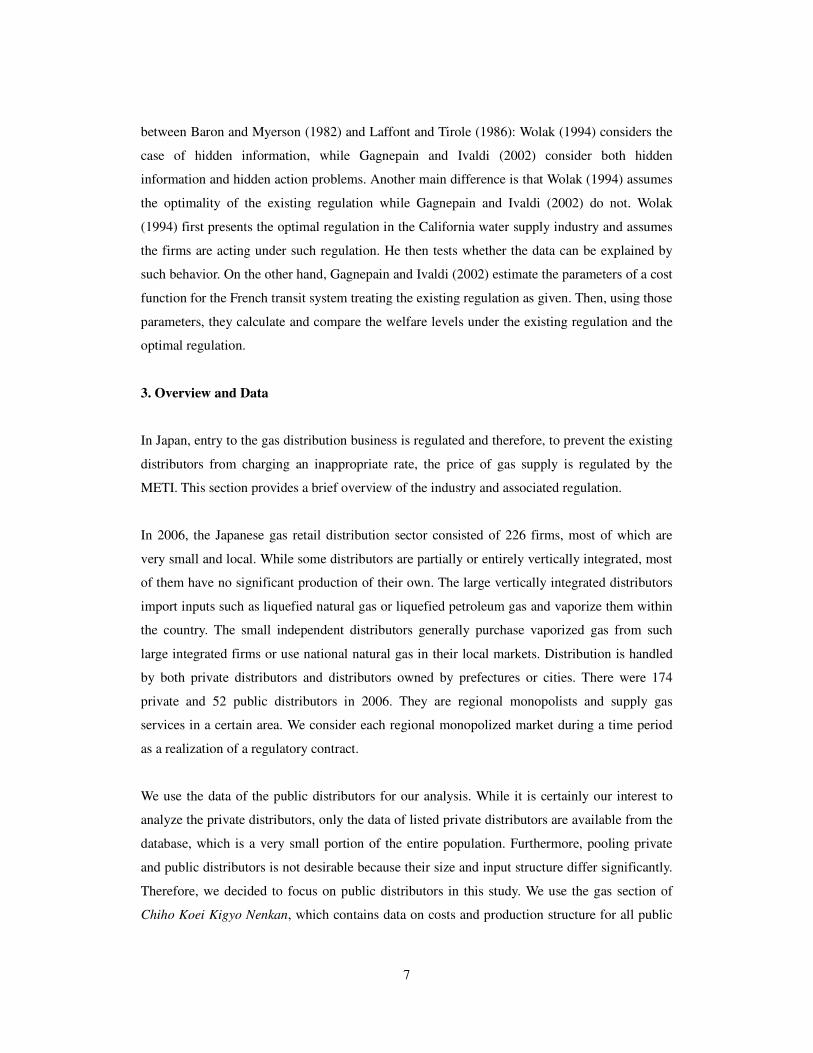
7
between Baron and Myerson (1982) and Laffont and Tirole (1986): Wolak (1994) considers the
case of hidden information, while Gagnepain and Ivaldi (2002) consider both hidden
information and hidden action problems. Another main difference is that Wolak (1994) assumes
the optimality of the existing regulation while Gagnepain and Ivaldi (2002) do not. Wolak
(1994) first presents the optimal regulation in the California water supply industry and assumes
the firms are acting under such regulation. He then tests whether the data can be explained by
such behavior. On the other hand, Gagnepain and Ivaldi (2002) estimate the parameters of a cost
function for the French transit system treating the existing regulation as given. Then, using those
parameters, they calculate and compare the welfare levels under the existing regulation and the
optimal regulation.
3. Overview and Data
In Japan, entry to the gas distribution business is regulated and therefore, to prevent the existing
distributors from charging an inappropriate rate, the price of gas supply is regulated by the
METI. This section provides a brief overview of the industry and associated regulation.
In 2006, the Japanese gas retail distribution sector consisted of 226 firms, most of which are
very small and local. While some distributors are partially or entirely vertically integrated, most
of them have no significant production of their own. The large vertically integrated distributors
import inputs such as liquefied natural gas or liquefied petroleum gas and vaporize them within
the country. The small independent distributors generally purchase vaporized gas from such
large integrated firms or use national natural gas in their local markets. Distribution is handled
by both private distributors and distributors owned by prefectures or cities. There were 174
private and 52 public distributors in 2006. They are regional monopolists and supply gas
services in a certain area. We consider each regional monopolized market during a time period
as a realization of a regulatory contract.
We use the data of the public distributors for our analysis. While it is certainly our interest to
analyze the private distributors, only the data of listed private distributors are available from the
database, which is a very small portion of the entire population. Furthermore, pooling private
and public distributors is not desirable because their size and input structure differ significantly.
Therefore, we decided to focus on public distributors in this study. We use the gas section of
Chiho Koei Kigyo Nenkan, which contains data on costs and production structure for all public

8
companies in Japan. Unless otherwise noted, data are taken from this source. This provides us
with a sample of 76 public gas distributors for the period 1990–2005.
Our sample can be classified into three categories according to technology. The first type does
not have any vaporization or reformer systems and purchases vaporized gas from large
integrated distributors or uses national natural gas. The second type includes those with
vaporization systems. They purchase liquefied natural gas from large distributors and vaporize it
on site. The last type owns reformer systems that enable them to convert liquefied petroleum gas
to city gas. The gas jigyo binran states how each distributor is classified. Because of the
technological differences, the cost structures of the three types differ significantly. For example,
the first type incurs low input costs as vaporized gas is transported through conduits, while the
second type transports liquefied natural gas by tank trucks, which is very costly. Therefore, for
the purpose of homogeneity, we use only the first type of distributors for the estimation of the
cost function. This leaves us with an unbalanced panel of 59 distributors for the estimation in
the sample period.
Japanese gas retail distributors need to obtain permission from the METI when they change
price.4 Based on the expected future demand for a certain number of coming years (one year for
the existing distributors, three years for the new distributors), price rP is determined to satisfy
the equation below:
sBYCYPeer += )( , (1)
where eY is the expected demand, )( eYC is the expected operating cost to meet the expected
demand, s is the rate of return, and B is the rate base. Specifically, for private distributors, s is
the weighted average of the rates of return on equity capital and liability, and B is the sum of
operational capital and fixed assets. For public distributors, sB is the interest expense on
enterprise loans, temporary loans and money transferred, plus less than 2 percent of the average
4 This requirement has been abolished for voluntary price reductions since 1998. Distributors are only
required to report in the case of voluntary price reduction. (There have been, however, only two cases of
such voluntary price reduction among our samples during the sample period. Non-voluntary price
reduction includes those due to structural change such as calorific value change. In such cases with
structural changes, distributors still need to obtain permission for a price reduction). Furthermore, for
large suppliers, entry and pricing have been deregulated since 1995. Our study focuses on small supply
services that are still under regulation.
9
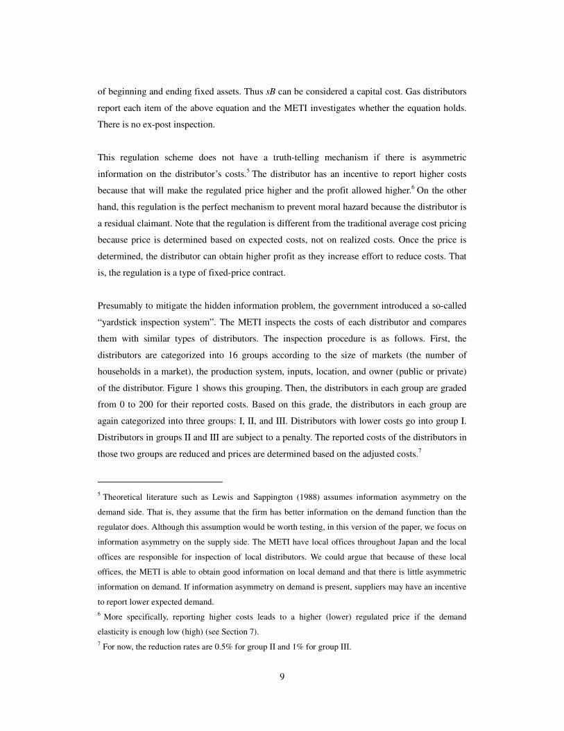
of beginning and ending fixed assets. Thus sB can be considered a capital cost. Gas distributors
report each item of the above equation and the METI investigates whether the equation holds.
There is no ex-post inspection.
This regulation scheme does not have a truth-telling mechanism if there is asymmetric
information on the distributor’s costs.5 The distributor has an incentive to report higher costs
because that will make the regulated price higher and the profit allowed higher.6 On the other
hand, this regulation is the perfect mechanism to prevent moral hazard because the distributor is
a residual claimant. Note that the regulation is different from the traditional average cost pricing
because price is determined based on expected costs, not on realized costs. Once the price is
determined, the distributor can obtain higher profit as they increase effort to reduce costs. That
is, the regulation is a type of fixed-price contract.
Presumably to mitigate the hidden information problem, the government introduced a so-called
“yardstick inspection system”. The METI inspects the costs of each distributor and compares
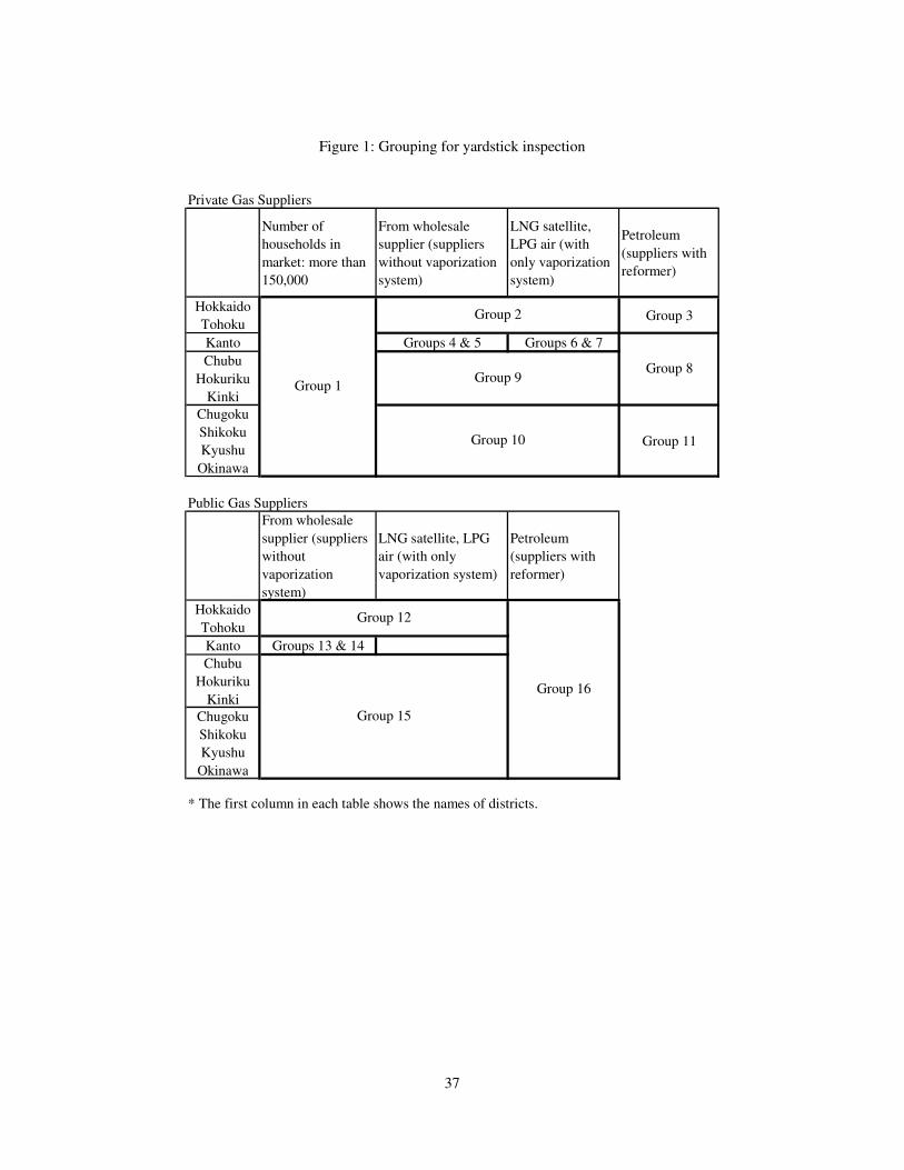
them with similar types of distributors. The inspection procedure is as follows. First, the
distributors are categorized into 16 groups according to the size of markets (the number of
households in a market), the production system, inputs, location, and owner (public or private)
of the distributor. Figure 1 shows this grouping. Then, the distributors in each group are graded
from 0 to 200 for their reported costs. Based on this grade, the distributors in each group are
again categorized into three groups: I, II, and III. Distributors with lower costs go into group I.
Distributors in groups II and III are subject to a penalty. The reported costs of the distributors in
those two groups are reduced and prices are determined based on the adjusted costs.7
5 Theoretical literature such as Lewis and Sappington (1988) assumes information asymmetry on the
demand side. That is, they assume that the firm has better information on the demand function than the
regulator does. Although this assumption would be worth testing, in this version of the paper, we focus on
information asymmetry on the supply side. The METI have local offices throughout Japan and the local
offices are responsible for inspection of local distributors. We could argue that because of these local
offices, the METI is able to obtain good information on local demand and that there is little asymmetric
information on demand. If information asymmetry on demand is present, suppliers may have an incentive
to report lower expected demand.
6 More specifically, reporting higher costs leads to a higher (lower) regulated price if the demand
elasticity is enough low (high) (see Section 7).
7 For now, the reduction rates are 0.5% for group II and 1% for group III.

10
<<Insert figure 1 about here>>
Although Japanese yardstick inspection is not identical to the textbook type of yardstick
competition, it does have its essence. If the penalty is large enough, the regulation reduces the
incentive of firms to report higher costs (given firms in each group are actually very similar)
because if a firm lies and others report the truth, then the firm that lied will be punished. Thus,
the current regulation, which combines a yardstick and a fixed-price contract, theoretically
eliminates both adverse selection and moral hazard problems: yardstick inspection removes the
adverse selection problem while a fixed-price contract removes the moral hazard problem. In
addition, because a yardstick system does not require the regulator to give firms an
informational rent to tell the truth, the current regulation may indeed lead the industry to the
full-information outcome.89
In practice, however, it seems difficult for the yardstick system to work perfectly to remove the
adverse selection problem. First, it has often been discussed that the regulator is unlikely to find
a large set of truly identical firms. In this Japanese system, distributors cannot be identical even
in the same group. Second, again as an often-discussed point, firms may collude. Third, the
current penalty seems to be ad hoc. It is unclear if it is sufficiently high to induce truth telling.
Furthermore, here, the extent of the punishment depends only on the order of the costs, not on
the difference in the costs. This may also reduce the effectiveness of the regulation.
Because yardstick inspection is unlikely to work perfectly, we do not assume optimality of the
current regulation. Therefore, our estimation follows Gagnepain and Ivaldi (2002) rather than
Wolak (1994). This estimation requires only ex-post realized data and we do not have to model
the firms’ ex-ante behavior under yardstick inspection. This suits us because we are not sure to
what extent the Japanese yardstick is effective and therefore, how the firms behave under such
regulation: we cannot model ex-ante behavior of the firms. As described before, we infer such
ex-ante behavior of firms, truth telling or not, by the welfare difference.
8 With an individual incentive regulation, the regulator cannot achieve the full-information outcome
because it needs to give informational rents to firms, and usually such rents are costly.
9 We mean, by full-information outcome, the counterfactual outcome that can be achieved if the regulator
does not face the information disadvantage. This differs from the often-discussed first best outcome
because the regulator here is not a welfare maximizer. See Section 7 for the discussion of the Japanese
regulator’s objective.

11
All the gas distribution companies were surveyed in the first yardstick inspection in 1995. They
were required to provide values for the variables in equation (1), regardless of whether they
were willing to change their current prices. Following the first inspection, only the distributors
that applied for a price change are subject to yardstick inspection. Among our sample of 59
distributors, there were 14 applications for price changes subject to the yardstick after 1995, one
each in 2000 and 2003, two in 2001, four in 2004, and six in 2005. When only the distributors
that applied for a price change are inspected, the latest reported costs of firms that did not apply
for a price change (they did not report current costs) are used as a benchmark.
Figure 2 shows the average unit price of public firms over 1990–2005. The prices of public
firms have a downward trend after the introduction of yardstick inspection. There is a large drop
in prices in 1996, following the introduction of yardstick inspection.
<<Insert figure 2 about here>>
4. Theoretical Model
In this section, we consider a model of retail gas distribution services, which is still under price
regulation.10 To derive a structural model of the industry, we need a detailed account of the
technological, informational, and regulatory constraints. We start this section by describing our
assumptions on these constraints.
For the technological constraint, we assume that, to provide the required level of services,
denoted by Y, the gas distributor needs to combine four inputs: labor (L), gas (G), materials (M),
and capital (K). L includes all types of workers; G corresponds to gas inputs for distribution; K
refers to plant, infrastructure, and distribution networks; and M includes all materials used for
performing maintenance and management activities. The distribution process is then represented
as:
),,,( bKMGLfY = , (2)
where b is a vector of parameters characterizing the technology in the production process.
10 As noted, prices for large supply services were deregulated in 1995.
12
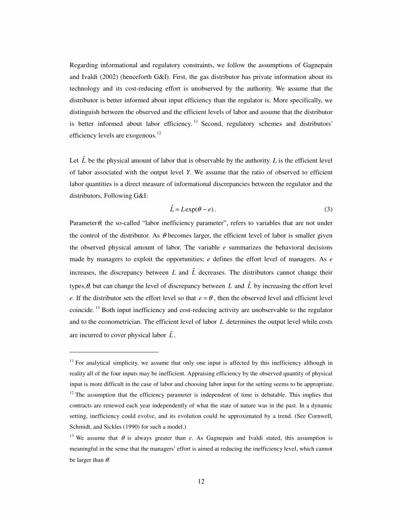
Regarding informational and regulatory constraints, we follow the assumptions of Gagnepain
and Ivaldi (2002) (henceforth G&I). First, the gas distributor has private information about its
technology and its cost-reducing effort is unobserved by the authority. We assume that the
distributor is better informed about input efficiency than the regulator is. More specifically, we
distinguish between the observed and the efficient levels of labor and assume that the distributor
is better informed about labor efficiency. 11 Second, regulatory schemes and distributors’
efficiency levels are exogenous.12
Let L be the physical amount of labor that is observable by the authority. L is the efficient level
of labor associated with the output level Y. We assume that the ratio of observed to efficient
labor quantities is a direct measure of informational discrepancies between the regulator and the
distributors. Following G&I:
)exp(ˆ eLL −= θ . (3)
Parameterθ, the so-called “labor inefficiency parameter”, refers to variables that are not under
the control of the distributor. As θ becomes larger, the efficient level of labor is smaller given
the observed physical amount of labor. The variable e summarizes the behavioral decisions
made by managers to exploit the opportunities; e defines the effort level of managers. As e
increases, the discrepancy between L and L decreases. The distributors cannot change their
types,θ, but can change the level of discrepancy between L and L by increasing the effort level
e. If the distributor sets the effort level so that θ=e , then the observed level and efficient level
coincide. 13 Both input inefficiency and cost-reducing activity are unobservable to the regulator
and to the econometrician. The efficient level of labor L determines the output level while costs
are incurred to cover physical labor L .
11 For analytical simplicity, we assume that only one input is affected by this inefficiency although in
reality all of the four inputs may be inefficient. Appraising efficiency by the observed quantity of physical
input is more difficult in the case of labor and choosing labor input for the setting seems to be appropriate.
12 The assumption that the efficiency parameter is independent of time is debatable. This implies that
contracts are renewed each year independently of what the state of nature was in the past. In a dynamic
setting, inefficiency could evolve, and its evolution could be approximated by a trend. (See Cornwell,
Schmidt, and Sickles (1990) for such a model.)
13 We assume that θ is always greater than e. As Gagnepain and Ivaldi stated, this assumption is
meaningful in the sense that the managers’ effort is aimed at reducing the inefficiency level, which cannot
be larger than θ.

13
Next, we interpret the distributors’ decision process after the price is set. The decision process
consists of choosing the optimal input and effort allocation. Note that this is an ex-post behavior
and does not involve an ex-ante decision process, such as which level of costs to report, under
the yardstick regulatory environment. We decompose this ex-post decision process into two
steps. The first step is to choose the optimal input and the second is to choose the optimal effort
allocation, given the regulated price and the demand associated with the price.
Assuming that the distributor is a price-taker in the market for input factors and has a cost-
minimizing behavior for each level of effort, an operating cost function can represent the
technological process. The operating cost faced by the distributor is:
MGLCMGL
ωωω ++= ˆ ,
where ],,[MGL
ωωωω = are the prices of labor, gas, and materials, respectively. We assume that
K cannot be fully adjusted in the short run and is fixed. 14 From duality theory, the conditional
operating cost function is defined by:
MGeLeKYCMGLMGL
ωωθωβθω ++−= )exp(min),,,,( ,, , (4)
subject to:
).,,,( bKMGLfY =
Equation (4) defines a “conditional” operating cost function because it still contains a level of
effort. This is the first step in the distributors’ decision process.
The second step is to determine the level of cost-reducing activity under the given regulatory
environment. As seen in the previous section, the Japanese authority sets the price of gas
services so that it equals the expected average cost (see equation 1). There is no ex-post
inspection to check whether the reported cost is actually equal to the realized cost. Under this
fixed-price regulation, the distributor is the residual claimant of effort. After the activity in the
contractual period, all the realized profit goes to the distributor. The utility of the firm is given
by:
),(),,,,()( esBeKYCYYPU ψβθω −−−= (5)
where )(eψ is the cost of effort function; exhibiting effort is costly for the firm. The distributor
14 We also assume that the capital cost sB is fixed in the short term and therefore it is included not in the
operating costs but in the total cost.

14
maximizes utility in equation (5) with respect to the effort level, e , and the first-order condition
is:
eCe ∂−∂= /)('ψ , (6)
which implies that the marginal cost of effort equals the marginal cost saving from the effort.
5. Empirical Model
5.1 Functional forms
We choose a simple Cobb–Douglas function to represent technology for the following reasons.
First, we use it for tractability. Although we could have used more elaborate functional forms
such as a translog for the estimation of the cost function, computations of welfare become
cumbersome with such functions. Second, because of the choice of the Cobb–Douglas function,
the two-step decision process above (the input allocation and effort level determination
problems) provides the same solution as if we had solved the two steps simultaneously. Under
Cobb–Douglas technology, the dual cost function is given by:
YKMGL YKeCMGLL
βββββωωωθββ )](exp[0 −= , (7)
with the assumption of homogeneity of degree one in input prices, that is 1=++MGL
βββ . We
should note that no constraint is imposed on the return to scale effect. As in previous studies, we
specify the cost of effort by:
1)exp()( −= ee αψ , (8)
with α > 0.
Using these functional forms and the first-order condition (6), we can solve for the effort level
as:
.lnlnlnlnlnlnln 0*
L
YKMMGGLLLLYK
eβα
ββωβωβωβαββθβ
+
+++++−+= (9)
From the equation above, we can see that the equilibrium effort level under this regulation
regime is an increasing function in the inefficiency parameter θ, the output level Y, and the input
prices ,,GL
ωω and M
ω . A distributor with the larger θ (less efficient distributor) needs to make
a greater effort under this regulatory scheme. Moreover, *e is a decreasing function of α, the
technological parameter of the internal cost function (8).
Substituting the optimal effort level *e into the cost function (7) and taking the logarithm, we
15
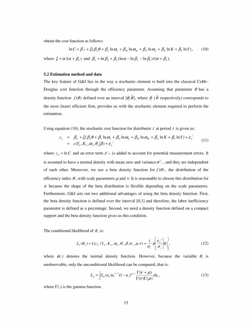
obtain the cost function as follows:
)lnlnlnlnln(ln 0'
YKCYKGGMMLLL
ββωβωβωβθβξβ ++++++= , (10)
where )/(L
βααξ += and )./()lnln(lnln 00
'
0 LLLβαββαβββ +−−+=
5.2 Estimation method and data
The key feature of G&I lies in the way a stochastic element is built into the classical Cobb–
Douglas cost function through the efficiency parameter. Assuming that parameter θ has a
density function )(θf defined over an interval ],[ θθ , where θ (θ respectively) corresponds to
the most (least) efficient firm, provides us with the stochastic element required to perform the
estimation.
Using equation (10), the stochastic cost function for distributor i at period t is given as:
c
ititititit
c
itYKMMGGLLLit
KYc
YKc
εβθω
εββωβωβωβθβξβ
+=
+++++++=
),,,(
)lnlnlnlnln('
0 (11)
where Ccit
ln= and an error term itcε is added to account for potential measurement errors. It
is assumed to have a normal density with mean zero and variance c2σ , and they are independent
of each other. Moreover, we use a beta density function for )(θf , the distribution of the
efficiency index θ , with scale parameters µ and ν. It is reasonable to choose this distribution for
θ because the shape of the beta distribution is flexible depending on the scale parameters.
Furthermore, G&I sets out two additional advantages of using the beta density function. First,
the beta density function is defined over the interval [0,1] and therefore, the labor inefficiency
parameter is defined as a percentage. Second, we need a density function defined on a compact
support and the beta density function gives us this condition.
The conditional likelihood of i
θ is:
,1
),,,,,,,|()(
== i
c
c
it
c
ciitititititit KYcLL θσ
εφ
σνµσβθωθ (12)
where (.)φ denotes the normal density function. However, because the variable i
θ is
unobservable, only the unconditional likelihood can be computed, that is:
∫ΓΓ
+Γ−= −−
1
0
11,
)()(
)()1()(
iiiiititduuuuLL
µν
µνµν (13)
where Γ(.) is the gamma function.
16
The sample consists of 76 public gas distributors for the period 1990–2005. As described in
Section 3, the sample can be categorized into three types according to their technology. For the
cost estimation, we use 59 distributors of Type 1 for the purpose of homogeneity. Estimating the
Cobb–Douglas cost function requires measures of the level of operating costs, the quantity of
output, and the input prices. The output is specified as total volume (m³) of gas supplied by
distributors. The total length of the conduit (m) is used for the quantity of capital. Costs of labor
are specified as total labor expenditures including wages, salaries, pensions, and benefits. The
price of labor is calculated as labor costs divided by the number of employees. Costs of
materials are specified as nonpersonnel expenses for day-to-day operations and maintenance of
the distribution network. The price of materials is calculated as the costs of materials divided by
the number of meters (that is, the number of households that have access to the gas supply
service) in each market. Because the costs of materials mostly arise from operating and
maintaining distribution lines to households, the number of households seems to be a suitable
measure of material inputs. Costs of gas input are specified as total expenditure on raw material
inputs. The price of gas is calculated as the costs of gas divided by the total amount of gas used
for distribution.
For welfare analysis, we estimate the demand function in Section 7. We use all 76 samples for
the demand estimation. This estimation additionally requires measures of consumer prices. We
use the calorific value-adjusted price (yen/10,000 kcal) as the price measure. Furthermore,
welfare calculation requires the capital cost, sB in equation (1). Capital cost is specified as
interest expenses on enterprise loans, temporary loans, and money transferred plus 2 percent of
the average of the beginning and ending fixed assets.
Summary statistics of the variables categorized according to their technology types are given in
Table 1.
Table 2 compares the average operating costs and prices before and after the introduction of
yardstick inspection. We can see from the last row that, in our sample, both the mean average
operating cost and the mean price decreased after the introduction of yardstick competition.
These changes are statistically significant. The standard deviations of costs and prices also
decreased after the introduction of yardstick inspection, although the latter is statistically
insignificant. We examine these statistics in each group of the yardstick inspection; however,

17
some groups show different changes. In group 15, the mean of prices increased, despite a
decrease in the mean of costs, after the introduction of yardstick inspection. In groups 12 and 15,
the standard deviations of prices increased after the introduction of yardstick competition.
Furthermore, Table 2 compares the mean growth rates of average cost before and after the
introduction of yardstick inspection. We can see from the last row that, in our sample, the
average operating costs were decreasing in the sample period. These decreases are not
significantly different between the two periods at 5 percent level. In group 14, however, average
operating costs were increasing before the introduction of yardstick inspection, while they were
decreasing afterward.
6. Estimation Results
6.1 Estimation results of cost function
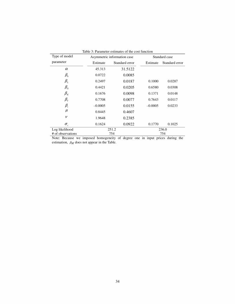
The estimated parameter values for equation (11) are reported in Table 3. Because we assumed
homogeneity, the parameter for M
β is dropped. To capture the time trend, we add a year dummy
to equation (11), and t
β denotes its coefficient.
All parameters are significant at least 10 percent level, except α andt
β . In particular, this is true
for the scale parameters µ and ν characterizing the density of the inefficiency level. From the
estimated µ and ν, it turns out that the density function is a decreasing function. More than 70
percent of the distributors have a θ of less than 0.5.
Along with the above model, we also estimate the alternative model. The alternative model is a
Cobb–Douglas cost function that does not take into account regulatory and informational
constraints. This model is referred to as the standard case, namely:
.lnlnlnlnlnlnln,,,0
c
ittitKitYitGGitMMitLLiitYearKYC εβββωβωβωββ +++++++= (14)
The standard case includes a time trend and a firm effect i0β to allow for a fixed-effect
estimation procedure. To compare the fit of the two models, we conducted a Vuong (1989) test
whose null hypothesis is that the two models are equally far from the true data-generating
process in terms of Kullback–Liebler distances. The alternative hypothesis is that one of the two
models is closer to the true data-generating process. We obtain a Vuong statistic of 2.67. This
statistically supports the asymmetric information model generated by the structural approach
rather than the standard model.
18
6.2 Efficiency and effort levels
Estimates of individual efficiency parameters can also be recovered. From equations (10) and
(11), the error term of the cost function has two unobservable, random, and independent
components, i
θ andc
itε . The error term can be written as:
iL
c
ititu θξβε += ,
where )/(L
βααξ += . From a procedure by Jondrow et al. (1982), we recover an estimate for
each i
θ from the values of residuals it
u by considering the conditional distribution of i
θ given
itu , that is, by computing )|(ˆ
ititiuE θθ = . For all distributors in our data set, the estimated
values of the efficiency levels are available from the authors. Once the estimate for i
θ is
obtained, we can then also obtain the effort level using equation (9).
From equation (7), the cost distortion that measures the discrepancy between the theoretical
frontier and the observed cost is given by:
)](exp[ eL
−θβ . (15)
The maximum cost distortion is achieved for a zero level of effort and an inefficiency level
equal to one. Figure 3 presents our set of distributors in 1996 ranked according to their cost
distortions defined by equation (15). In addition, Figure 3 provides the level of the inefficiency
parameter for each distributor. Reflecting the high efficiency levels and the high-powered
incentive regulatory scheme (that is, fixed-price contract), the distortion is not very high. The
maximum distortion is about 10.1 percent, and most of the distributors exhibit a distortion level
of less than 5 percent.
<<Insert figure 3 about here>>
7. Welfare Implications and the Effect of Yardstick Inspection
7.1 Demand
Our objective is now to perform a comparison of current and full-information welfare. First, to
compute consumer surplus, the price elasticity of demand must be estimated.
Assume the demand function is log linear such that:
dtdPddY ε+++= 210 lnln , (16)

19
where a vector 0d includes the fixed effects and t is a year dummy. Our model of costs and the
demand systems is sequential. First, the government sets a price and once the price is known,
the demand level is determined according to equation (16). Finally, the cost of running the
service is obtained through the cost model given by equation (10). This gives rise to a block-
recursive structure, so each equation can be estimated separately. We obtained the estimated
results of price elasticity 0.275. See Table 4 for the results.
7.2 Regulator’s behavior
We now know the cost structure, the demand elasticity, the inefficiency level, the effort function,
and the price level. Additionally, the behavior of the regulator must be specified. Here, we
consider the regulator’s pricing behavior, ignoring the existence of the yardstick regulation for
now. As noted in Section 3, the regulation requires the price to be equal to an expected average
cost as in equation (1): eerYsBYCP /))(( += . Therefore, we assume that the regulator’s
objective is to set the price equal to the average cost such that:
sBYCYPr += )( , (17)
where Y is the realized output level.15 Given the selected price is a point on the inverse demand
function, (.)P , when the authority has set the price, the associated demand Y is implicitly
determined, that is, the customers adjust their demand at this price. The regulator should take
this into account and therefore, equation (17) can be rewritten as:
sBeKYC
sBYCYYP
+=
+=
),,,,(
)()(
βθω (18)
where the cost function in equation (4) is substituted. The regulator’s problem is to find the
demand level Y that satisfies the equation above, given ,,,,, βθω eK and sB .
We assume that the regulator observes all the variables and the parameters in the above equation
except θ and e. Actually, however, from equation (9), once the level of Y is determined, the
level of effort can be recovered if θ is recovered: )|,,,(* βθωKYee = . The regulator is
assumed to know this structure of the industry and therefore, the only unobservable for the
15 Gagnepain and Ivaldi (2002) assume that the regulator is a welfare maximizer, given the regulatory
environment. However, because it is not welfare maximizing to set the price to be equal to the average
cost, we do not assume it here. Therefore, our full-information welfare is different from the first-best
welfare unlike often discussed, and the current welfare may be larger than the full-information welfare.

20
regulator is θ .
Given the above assumptions, the regulatory environment is reduced to the following. First, the
distributor reports the levels of θω,,K and sB , and the regulator sets the level of output so that
equation (18) holds, given the reported levels. Because sBK , and ω are observed by the
regulator, we assume that the distributor reports the true levels of these variables; they are the
same as the observed data. On the other hand, because the regulator does not observe the level
of θ , we distinguish the true level of θ from the reported level θ . We assume that the
regulator believes that θθ =ˆ . Given the reported inefficiency level θ , the regulated output level
rY is determined so that:
sBYKKYe
sBKYeKYCYYPY
KMGL r
MGL
r
L
rrrr
+−=
+=βββββ ωωωβθωθββ
βθβθωω
))]|ˆ,,,(ˆ(exp[
)|ˆ),|ˆ,,,(,,,()(*
0
*
(19)
where .lnlnlnlnlnlnlnˆ
)|ˆ,,,( 0*
L
r
YKMMGGLLLLr YKKYe
βα
ββωβωβωβαββθββθω
+
+++++−+=
We can see that the regulated output level can be expressed as a function of the reported
inefficiency level: )ˆ(θYYr = .
7.3 Ex-post distributor’s behavior
Once the regulated output level )ˆ(θYYr = is determined, the distributor conducts cost-
minimization activity (4) given )ˆ(θY and for each level of effort e , and the cost function is
described as a function of both θ and θ , namely:
YKMGL YKeeYC MGLL
βββββθωωωθββθθ )ˆ()](exp[)|)ˆ(,( 0 −= . (20)
Similarly, the distributor next maximizes utility with respect to the effort level given the
regulated output level )ˆ(θY , and the first-order condition (9) gives us the effort level as a
function of both θ and θ , namely:
.)ˆ(lnlnlnlnlnlnln
))ˆ(,( 0*
L
YKMMGGLLLL YKYe
βα
θββωβωβωβαββθβθθ
+
+++++−+= (21)
Therefore, the cost realization will be as the following,
YKMGL YKYeYeYC MGLL
βββββθωωωθθθββθθθθ )ˆ()))]ˆ(,((exp[)))ˆ(,(),ˆ(,( *
0* −= (22)
7.4 Welfare implications
Given our knowledge of the demand and supply functions, we now calculate the welfare levels

21
under the current and the hypothetical full-information situations to see whether the introduction
of yardstick inspection reduces the information disadvantage of the regulator. Full-information
welfare is obtained by assuming the regulator observes all the variables and parameters.
We define social welfare as:
URSW +−= (23)
where S is the gross surplus and derived from the demand function, R is the distributor’s
revenue and obtained as the product of the price and the demand level, and U is the firm’s utility
defined in equation (4).
Substituting (21) and (22), the current (actual) welfare level cW can be expressed, given the
reported inefficiency level θ and the true inefficiency level θ , as follows:
)))]ˆ(,(()))ˆ(,(),ˆ(,()ˆ())ˆ(([)ˆ())ˆ(())ˆ(()ˆ,( ** θθψθθθθθθθθθθθ YesBYeYCYYPYYPYSWc −−−+−= (24)
This can be calculated by using the observed output level for )ˆ(θY and the inefficiency level θ
recovered in Subsection 6.2. The full-information welfare level fW , which can be obtained if a
distributor reports the true inefficiency level θ , that is, if θθ =ˆ , is:
)))](,(()))(,(),(,()())(([)())(())((
),(** θθψθθθθθθθθθ
θθ
YesBYeYCYYPYYPYS
WWcf
−−−+−=
= (25)
The problem with the fixed-price contract is that it does not have any truth-telling mechanism.
Therefore, the distributors may have an incentive to report θ , which is higher than the true level
θ , to obtain a higher permitted profit. Such a behavior either decreases or increases social
welfare away from the full-information welfare.16 Appendix A shows that reporting a higher
inefficiency level θ leads to a higher (lower) regulated price and lower (higher) output if the
slope of the inverse demand curve is smaller (larger) than the average cost curve. It turns out
that with our estimated parameter values, all our observed markets exhibit a smaller slope of the
inverse demand curve than that of the average cost curve. Figure 4 describes this situation. In
Figure 4, θAC is the true average cost curve of a firm with inefficiency level θ , and θ
AC is the
false average cost curve the regulator believes that the firm has when the firm reports θ such
16 As noted, the full-information welfare is different from the often-discussed first best welfare. Therefore,
the current welfare can be higher than the full-information welfare.

22
that θθ ˆ< . That is:
,))]|,,,((exp[
)|),|,,,(,,,()(
*0
*
Y
YKKYe
Y
sBKYeKYCYAC
YKMGL
MGLL
βββββ
θ
ωωωβθωθββ
βθβθωω
−=
+=
where ,lnlnlnlnlnlnln
)|,,,(* 0
L
YKMMGGLLLL YKKYe
βα
ββωβωβωβαββθββθω
+
+++++−+= and
,))]|ˆ,,,(ˆ(exp[
)|ˆ),|ˆ,,,(,,,()(
*
0
*
ˆ
Y
YKKYe
Y
sBKYeKYCYAC
YKMGL
MGLL
βββββ
θ
ωωωβθωθββ
βθβθωω
−=
+=
where .lnlnlnlnlnlnlnˆ
)|ˆ,,,(* 0
L
YKMMGGLLLL YKKYe
βα
ββωβωβωβαββθββθω
+
+++++−+=
)(YP is the inverse demand function. In the full-information case, price is determined so that
θACP = . This price and the associated demand are shown by )(θP and )(θY , respectively, in
Figure 4. However, if the firm reports a higher θ , price and output are determined at the levels
of )ˆ(θP and )ˆ(θY in Figure 4. In such a case, the firm’s true average cost is ))ˆ(( θθ YAC given
the regulated output level )ˆ(θY . The firm’s profit increases from zero in the full-information
case to the area ))ˆ(()ˆ( θθ YadACP . The firm’s utility also increases, because the effort level
decreases because of the lower output. Consumer surplus decreases because of a higher price
and lower output.
<<Insert figure 4 about here>>
The introduction of yardstick inspection may reduce the incentive to report a higher θ , because
if a distributor reports a higher inefficiency level than the other distributors in the same group, it
is subject to penalty. In the next subsection, we show that if the yardstick inspection actually
reduces the discrepancy between θ and θ , the difference between cW in equation (24) and fW
in equation (25) should also decrease. We assess whether the introduction of yardstick
inspection actually reduces the discrepancy between θ and θ by examining whether the
discrepancy between cW and f
W has been reduced since its introduction.
7.5 The effect of yardstick inspection
The very first yardstick inspection was conducted in 1995. Under this first inspection, all gas

23
distributors were required to report values of the variables in equation (1), regardless of whether
they were willing to change their current prices at the time. Since the first inspection, only
distributors that apply for a price change have been subject to yardstick inspection. Among our
sample of 59 distributors, there were 14 applications for price changes that were subject to the
yardstick after 1995, one each in 2000 and 2003, two in 2001, four in 2004, and six in 2005.
We call the first inspection, in which all the distributors are targets, the “simultaneous yardstick
inspection” and the subsequent cases, in which the distributor that applied for a price change is
the target, as the “individual yardstick inspection”. We examine the difference between full-
information welfare fW in equation (25) and current welfare cW in equation (24) or
cfWWW −=∆ , with and without yardstick inspection. Equations (24) and (25) show that as a
reported inefficiency level converges to the true inefficiency level, the welfare difference
converges to zero. That is, as ,ˆ θθ → fcWW → and 0→∆W . Furthermore, Appendix B
shows that with our parameter estimates, current welfare )ˆ,( θθcW is a monotonically
decreasing function of θ . Therefore, the welfare difference cf WWW −=∆ is always positive
(when θθ >ˆ ) and an increasing function of θ . Therefore, if yardstick inspection has the effect
of reducing firms’ incentive to report higher inefficiency levels (that is, if yardstick inspection
has the effect of reducing the discrepancy between θ and θ ), it reduces W∆ .
We examine several measures of the effect of yardstick inspection, which are expected to take a
negative value if yardstick inspection has the effect of reducing firms’ incentive to report higher
inefficiency levels. Now, let R be the indicator variable such that 1=it
R if distributor i is
subject to yardstick inspection in year t and 0=it
R otherwise. Also, let I be the indicator
variable such that 1=it
I if distributor i applied for a price change and obtained permission in
year t and 0=it
I otherwise. That is, when 0=it
I , a distributor preferred the status quo. Our
first measure of the yardstick effect is:
][iiave
DiffEEffect = , (26)
where ]1&0|[]1|[ ==∆−=∆=itititititi
IRWERWEDiff for each i . This is a simple average
difference in the welfare disparity with and without yardstick inspection. Next, we examine the
effect of simultaneous yardstick inspection:
][ ,isimisimDiffEEffect = , (27)
where ]1&0|[]1995&1|[, ==∆−==∆=itititititisim
IRWEtRWEDiff for each i . This is an

24
average difference in the welfare disparity with and without simultaneous yardstick inspection.
Next, we examine the effect of individual yardstick inspection:
][ ,iindiindDiffEEffect = , (28)
where ]1&0|[]1995&1|[, ==∆−≠=∆=itititititiind
IRWEtRWEDiff for each i .
The results are shown in Table 5. We calculate both per-household welfare and total market
welfare in each market and calculate the measures of improvement in welfare disparity defined
above. The negative values imply that yardstick inspection reduced the adverse selection
problem. The first row of Table 5 shows the measure defined in equation (26). We can see that,
on average, yardstick inspection improved the per-household welfare disparity. On average, the
per-household welfare disparity from the full-information outcome is 26.40 yen smaller under
yardstick inspection. The second row shows the measure defined in equation (27). Again, we
can see that the per-household welfare disparity is 127.51 yen smaller under yardstick
inspection. This implies that the simultaneous yardstick inspection in 1995 was somewhat
effective in reducing adverse selection. Measures (26) and (27) calculated with total market
welfare, however, show that welfare disparity was widened by yardstick inspection. Total
market welfare disparity is 5,604,000 yen larger under yardstick inspection. It is 3,367,000 yen
larger under simultaneous yardstick inspection. The result that per-household welfare disparity
was improved while total market welfare disparity was not may imply that simultaneous
yardstick inspection was effective only for firms in small markets. Because our estimated cost
function exhibits scale economies, firms in large markets have a cost advantage. Therefore, our
results suggest that the simultaneous yardstick inspection was effective only for firms without a
cost advantage in reducing the adverse selection problem: firms with a cost advantage still have
incentive to report higher costs even under yardstick inspection, while firms without a cost
advantage have a lower incentive to report higher costs. One possible reason for such a
phenomenon is that firms are not identical in the yardstick comparison groups. Yardstick
grouping may not be appropriate here, and such a grouping may reduce the effect of yardstick
inspection.
The measure of the effect of independent yardstick inspections defined in equation (28) shows a
different result. On average, it can be seen from the third row that the individual yardstick
inspection widened both per-household and total market welfare disparities. The per-household
and total market welfare disparities widened, by 647.11 yen and 23,700,000 yen, respectively.
This implies that subsequent individual yardstick inspections do not always have the power to

25
reduce the adverse selection problem. Why might an individual case not work? One possible
reason is that, in such an individual case, the benchmark costs are already known for the firms
from the first inspection in 1995. Therefore, our results may give rise to a dynamic concern,
similar to the Ratchet effect, because the subsequent inspection cannot be effective for a firm
that has learned the relative position of its costs.
Finally, we calculate the additional two measures. The first measure simply looks at the average
difference in the welfare disparity before and after the introduction of yardstick inspection,
regardless of whether or not the firm is subject to yardstick inspection. Namely:
][ ,// iafterbeforeiafterbeforeDiffEEffect = , (30)
where ]1995|[]1995|[,/ >∆−≤∆= tWEtWEDiffititiafterbeofer
for each i . The second measure
looks at the average difference in the welfare disparity before and after the introduction of
yardstick inspection when firms choose the status quo. Namely:
][ ,.. iquostatusiquostatus DiffEEffect = , (31)
where ]0&1995|[]0&1995|[,. =>∆−=≤∆= ititititiquostatus ItWEItWEDiff for each i . We also
calculate these measures by groups. The results are shown in the last 12 rows in Table 5.
The fifth row in Table 5 (the measure defined in equation (30)) shows that, in general, the
welfare disparity from the full-information outcome widened after the introduction of yardstick
inspection in 1995. Specifically, the welfare disparity widened by 8,954,000 yen, while the per-
household welfare disparity widened by 341.27 yen after 1995. Similar results are observed in
all groups except group 12. If we compare the cases where firms kept the status quo (the
measure defined in equation (31)), we again find that the welfare disparity widened after the
introduction of yardstick inspection. Specifically, as shown in the 11th row, the welfare disparity
widened by 9,215,000 yen, while the per-household welfare disparity widened by 385.63 yen
after 1995. Again, similar results are observed in all groups except group 12.
Because costs were decreasing during our sample period, keeping the status quo must have led
to larger welfare disparity. Moreover, the higher the rate at which costs decrease, the larger the
welfare disparity is when a firm keeps the status quo. Therefore, the above results of the larger
welfare disparity after 1995 may merely reflect the higher rate of cost decrease in the period
after 1995. However, the larger disparity after 1995 is observed even in the groups where the
cost decrease rates are not significantly different between the periods before and after the

26
introduction of yardstick inspection (see Table 2 for the cost decrease rates). Therefore, our
results may imply that the introduction of yardstick inspection reduced firms’ incentive to adjust
prices.
Why might firms have less incentive to adjust prices under yardstick inspection? This may be
explained by firms’ collusive behavior. If a firm with decreased costs keeps the status quo, the
benchmark cost will be kept high, while if it adjusts prices, the regulator will recognize lower
costs and the benchmark cost will be reduced. Therefore, firms may have incentive to collude to
keep the status quo.
8. Conclusion
This study is aimed at assessing the effect of yardstick inspection in the Japanese retail gas
distribution industry. Realizing that yardstick inspection will lead the industry to the full-
information outcome if it works perfectly to eliminate the adverse selection problem, we infer
its effect from the difference between the current and the hypothetical full-information welfare
levels.
We estimate a cost function for gas distributors under the assumption of asymmetric information
between the regulator and the distributor for the efficient level of labor. It is assumed that the
regulator does not observe either the inefficiency level or the effort level of each distributor. As
the existing regulation has an incentive mechanism to induce the distributor’s effort, the
distributor is assumed to maximize the utility with respect to the effort level. Therefore, the
effort level can be solved as a function of the parameters. Using distributional assumption
regarding the inefficiency level, maximum likelihood estimation is conducted to estimate the
parameters, except the inefficiency level, and then, the inefficiency level is recovered by the
method in Jondrow et al. (1982). It was shown that most distributors were quite efficient.
Having obtained all the parameters, the welfare levels under the current and the full-information
situations are calculated. Our results indicate that the welfare difference between the current and
the full-information outcomes is somewhat reduced by yardstick inspection on average,
implying that the inspection reduced firms’ incentive to report higher costs.
Yardstick inspection was introduced in 1995. In that year, all the firms were required to report
their costs for comparison. Since then, only the firms that apply for a price change are subject to

27
inspection and the most recent costs of the other firms (which do not apply for a price rise and
do not report costs) are used as the benchmark. Our results show that the initial inspection in
1995 reduced the welfare discrepancy, while the later individual cases did not. This may give
rise to a dynamic concern, similar to the Ratchet effect, such that subsequent inspection cannot
be effective for a firm that has learned the relative position of its cost. Furthermore, the
inspection seems to have discouraged firms from changing prices. Our results from this study
suggest that a better form of regulation, which takes into account firms’ dynamic incentive,
should be considered.
28
Appendix I
We show that if the slope of the inverse demand curve is smaller than the average cost curve,
reporting a higher inefficiency level θ leads to a lower regulated price and higher output.
As in equation (19), the regulator set the regulated price so that :
sBYKKYe
sBKYeKYCYYPYKMGL r
MGL
r
L
rrrr
+−=
+=βββββ
ωωωβθωθββ
βθβθωω
))]|ˆ,,,(ˆ(exp[
)|ˆ),|ˆ,,,(,,,()(*
0
*
where
.lnlnlnlnlnlnlnˆ
)|ˆ,,,( 0*
L
r
YKMMGGLLLLr YKKYe
βα
ββωβωβωβαββθββθω
+
+++++−+=
By totally differentiating the above equation, we obtain:
Y
C
Y
CYPYYP
C
d
dY
y
L
L
Y
L
L
ββα
ββ
ββα
α
θ+
+−+
+=
)()('ˆ
Therefore, 0ˆ
<θd
dYif
222)('
Y
C
Y
C
Y
sBCYP
y
L
L
yβ
βα
ββ
+−+
+−< (30)
The left side of the above inequality is the slope of the inverse demand curve and the right side
is the slope of the average cost curve. Therefore, if the slope of the inverse demand curve is
smaller than the average cost curve, reporting a higher inefficiency level θ leads to a lower
regulated price and higher output.
We confirmed that, with our estimated parameter values, inequality (30) indeed holds in all the
markets of our observation for a broad range of output level.17
Appendix B
In this appendix, we show that current welfare )ˆ,( θθcW is a monotonically decreasing function
of θ .
17 Specifically, we have checked the range from the half to the double of the current output level.

29
Differentiating equation (24) byθ , we obtain the following:
θβα
βαα
βα
ββ
θ
θθˆ
]1
)exp(1
)1()([ˆ
)ˆ,( *
d
dY
Ye
YCYP
d
dW
L
Y
L
L
y
c
+−
+−−=
But we know, from Appendix A, that 0ˆ
<θd
dY. Therefore, 0
ˆ
)ˆ,(<
θ
θθ
d
dWc
if
0]1
)exp(1
)1()([)( * >+
−+
−−≡ΦY
eY
CYPYL
Y
L
L
yβα
βαα
βα
ββ
The value of the left hand side of the above inequality )(YΦ depends on the level ofY . With our
parameter values, we graphically confirmed that )(YΦ is always positive for all Y such
that )(θYY < . 18 That is, 0ˆ
)ˆ(<
θ
θ
d
dWfor all Y such that )(θYY < : welfare is monotonically
decreasing in θ for the level of Y such that )(θYY ≤ .19
18 The graphs are available from the author upon request.
19 Because Appendix A shows that reporting higher θ decreases Y, we only need to consider the range of
Y such that )(θYY < .

30
References
Antonioli, B., Filippini, M., 2001. The Use of a variable cost function in the regulation of the
Italian water industry. Utilities Policy 10, 181-187.
Auriol, E., Laffont, J.J., 1992. Regulation by duopoly. Journal of Economics and Management
Strategy. 1, 507–533.
Baron, D.P., Myerson, R.B., 1982. Regulating a monopolist with unknown costs. Econometrica
50, 911–930.
Chong, E., 2003. Yardstick competition vs. individual incentive regulation: What has the
theoretical literature to say? mimeo. ADIS and ATOM.
Cornwell, C., Schmidt, P., Sickles, R.C., 1990. Production frontiers with cross-sectional and
time-series variation in efficiency levels. Journal of Econometrics 46, 185–200.
Dalen, D.M., Gómez-Lobo, A., 2003. Yardstick on the road: Regulatory contracts and cost
efficiency in the Norwegian bus industry. Transportation 30, 371-386.
Farsi, M., Filippini, M., 2004. Regulation and measuring cost-efficiency with panel data
models: Application to electricity distribution utilities. Review of Industrial Organization
25, 1-19.
Gagnepain, P., Ivaldi, M., 2002. Incentive regulatory policies: the case of public transit systems
in France. RAND Journal of Economics 33, 605–629.
Jondrow, J., Konox Lovell, C.A., Materov, I.S., Schmidt, P., 1982. On the estimation of
technical inefficiency in the stochastic frontier production function model. Journal of
Econometrics 19, 233–238.
Laffont, J.J., Tirole, J., 1986. Using cost observation to regulate firms. Journal of Political
Economy 94, 614–641.
Lewis, T.R., Sappington, D.E.M., Regulating a monopolist with unknown demand. American
Economic Review 78, 986–998.
Potters, J., Rockenbach, B., Sadrieh,, A., van Damme, E., 2004. Collusion under yardstick
competition: an experimental study. International Journal of Industrial Organization 22,
1017-1038.
Shleifer, A., 1985. A Theory of yardstick competition. RAND Journal of Economics 16, 319–
327.
Tangerås, T.P., 2002. Collusion-proof yardstick competition. Journal of Public Economics 83,
231–254.
Vuong, Q., 1989. Likelihood ratio tests for model selection and non-nested hypotheses.
Econometrica 57, 307–334.

31
Wolak, F.A., 1994. An econometric analysis of the asymmetric information, regulator-utility
interaction. Annales d'Economie et de Statistique 34, 13–69.
Yatchew, A., 2001. Incentive regulation of distributing utilities using yardstick competition.
Electricity Journal 14, 56-60.

32
Table 1: Summary statistics
Production type
Output
(3m )
Total cost (1000 yen)
Labor price (1000 yen)
Material price (1000 yen)
Gas price
(1000 yen/3m )
Capital (m)
Consumer price
(yen/3m )
Capital cost (1000 yen)
Number of firms
1 Mean 9129486 673577 6869 14.825 0.0443 249432 112.414 136842 59 s.d. 14400000 949049 1433 10.069 0.0055 262417 26.263 96701 2 Mean 16400000 1681445 6990 20.114 0.0347 494968 152.705 1051975 21 s.d. 44000000 4198267 1424 9.413 0.0067 1112475 19.472 383928 3 Mean 15400000 1892904 7053 18.645 0.0355 848017 170.820 387286 3 s.d. 13700000 1568506 1457 8.999 0.0065 615647 12.212 446240
Total Mean 11100000 966965 6906 16.248 0.0418 334483 124.608 180327 76 s.d. 25000000 2262789 1432 10.125 0.0072 616029 31.346 545884
Note: Production type 1 includes those without vaporization systems or reformers. Type 2 includes those with vaporization systems. Type 3 includes those with reformers. The total number of firms is larger than the sum of the number of firms in each production type because some distributors switched their production type during the sample period.

33
Table 2: Cost and Price before and after the introduction of yardstick
Average operating cost (yen)
Price (yen)
Annual growth rate of average operating cost
(%)
Group Period Before After Before After Before After
Mean 129.65 120.57 *** 152.65 151.39 -0.780 -0.284 Group 12
S.D. 23.83 20.56 24.71 25.95 0.851 0.896
Mean 82.05 73.02 *** 105.87 101.77 *** -0.191 -1.591 Group 13 S.D. 26.31 14.89 *** 16.73 14.54 * 0.781 0.523 *
Mean 82.96 77.86 *** 101.66 97.99 0.467 -1.239 * Group 14 S.D. 12.00 14.48 * 16.22 13.95 0.585 0.453
Mean 86.81 83.18 123.00 124.05 -2.453 -1.951 Group 15
S.D. 6.16 24.57 *** 5.22 20.37 *** 1.084 1.714 *
Total Mean 92.21 82.24 *** 115.12 109.69 *** -0.244 -1.310 *
S.D. 29.55 23.47 *** 26.61 25.34 0.466 0.346
Note: The differences of means and standard deviations are tested by T-test and F-test, respectively. Stars refer to the significance. * = significant at the 10% level; ** = significant at the 5% level; and *** = significant at the 1% level.
34
Table 3: Parameter estimates of the cost function
Type of model Asymmetric information case Standard case
parameter Estimate Standard error Estimate Standard error
α 45.313 31.5122
0β 0.0722 0.0085
Lβ 0.2497 0.0187 0.1000 0.0287
Gβ 0.4421 0.0205 0.6580 0.0308
Kβ 0.1676 0.0098 0.1371 0.0148
Yβ 0.7708 0.0077 0.7643 0.0117
tβ –0.0005 0.0155 –0.0005 0.0233
µ 0.8445 0.4607
ν 1.9648 0.2385
cσ 0.1624 0.0922 0.1770 0.1025
Log likelihood 251.2 236.0 # of observations 754 754
Note: Because we imposed homogeneity of degree one in input prices during the
estimation, Mβ does not appear in the Table.

35
Table 4: Demand Estimation
Log output Coefficient Standard error
Log price -0.275 0.143 Constant 16.005 0.708 Fixed effect Yes Year dummy Yes
Number of Observation 1046 Adjusted R-squared 0.9696 F-test (91, 954) 367.61

36
Table 5: Welfare disparity between current and full information outcome:
Difference before and after the introduction of Yardstick
Measure
Per household
(yen) Whole market (thousand yen)
aveEffect –26.40 (62.02) 5604 (682)
simEffect –127.51 (62.16) 3363 (372)
indEffect 647.11 (143.18) 23700 (2142)
afterbeforeEffect ,
Total 341.27 (42.24) 8954 (285) Group 12 -19.47 (206.65) 297 (585) Group 13 448.35 (26.46) 5183 (197) Group 14 162.08 (48.95) 8857 (490) Group 15 1504.50 (76.82) 99300 (5236)
quostatusEffect .
Total 385.63 (48.97) 9215 (309) Group 12 -107.98 (245.21) -664 (667) Group 13 542.25 (28.48) 5664 (206) Group 14 197.37 (47.10) 9701 (519) Group 15 1527.86 (83.12) 98900 (5698)
Note: Negative value implies reduction in incentive to report higher cost. Inside the parentheses are standard errors.
37
Figure 1: Grouping for yardstick inspection
Private Gas Suppliers
Number of
households in
market: more than
150,000
From wholesale
supplier (suppliers
without vaporization
system)
LNG satellite,
LPG air (with
only vaporization
system)
Petroleum
(suppliers with
reformer)
Hokkaido
TohokuGroup 3
Kanto Groups 4 & 5 Groups 6 & 7
Chubu
Hokuriku
Kinki
Chugoku
Shikoku
Kyushu
Okinawa
Group 11
Public Gas Suppliers
From wholesale
supplier (suppliers
without
vaporization
system)
LNG satellite, LPG
air (with only
vaporization system)
Petroleum
(suppliers with
reformer)
Hokkaido
Tohoku
Kanto Groups 13 & 14
Chubu
Hokuriku
Kinki
Chugoku
Shikoku
Kyushu
Okinawa
* The first column in each table shows the names of districts.
Group 8
Group 12
Group 16
Group 15
Group 1
Group 2
Group 9
Group 10

38
Figure 2: Recent average unit price of public firms
119
120
121
122
123
124
125
126
127
128
1990
1992
1994
1996
1998
2000
2002
2004
year
unit p
rice
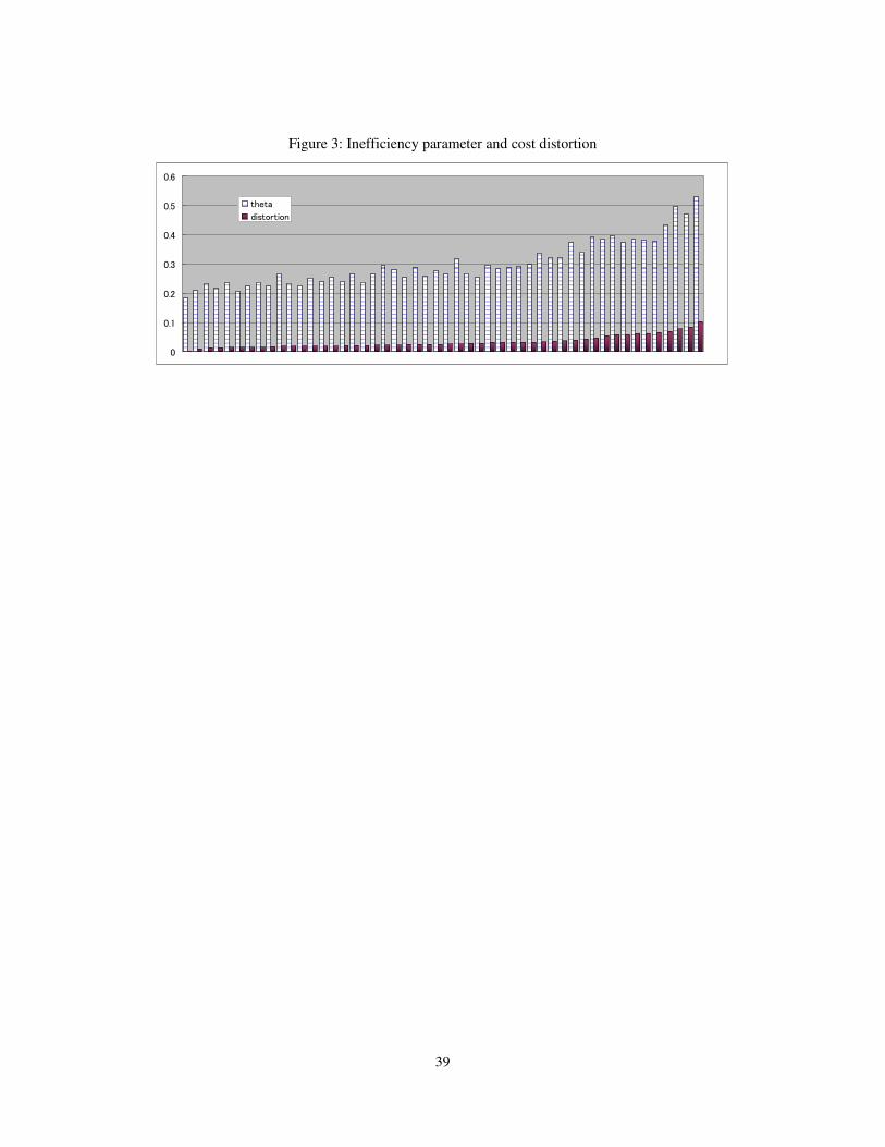
39
Figure 3: Inefficiency parameter and cost distortion
0
0.1
0.2
0.3
0.4
0.5
0.6
theta
distortion
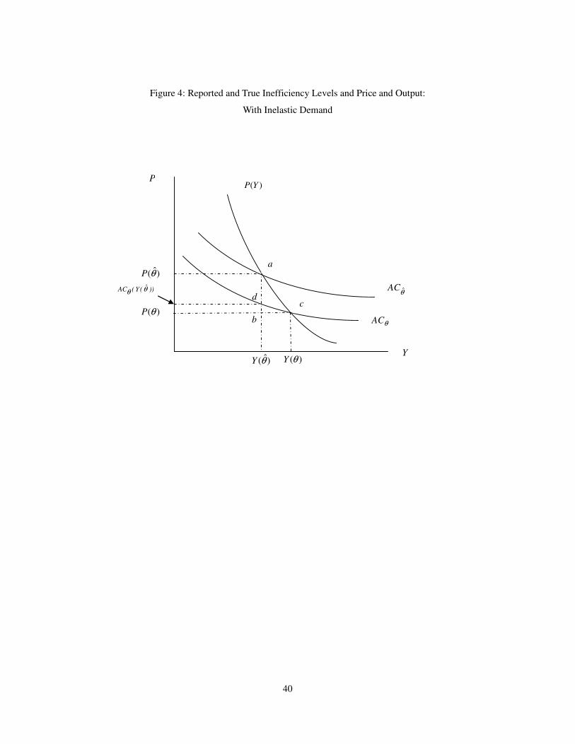
40
Figure 4: Reported and True Inefficiency Levels and Price and Output:
With Inelastic Demand
)ˆ(θY )(θY
b
d
P
Y
)(YP
θAC
θAC
a
c
)ˆ(θP
)(θP
))ˆ(Y(AC θθ