yi-fu cai et al- quintom cosmology: theoretical implications and observations
TRANSCRIPT

8/3/2019 Yi-Fu Cai et al- Quintom Cosmology: theoretical implications and observations
http://slidepdf.com/reader/full/yi-fu-cai-et-al-quintom-cosmology-theoretical-implications-and-observations 1/105
a r X i v : 0 9 0 9
. 2 7 7 6 v 2
[ h e p - t h ]
2 2 A p r 2 0 1 0
Quintom Cosmology: theoretical implications
and observations
Yi-Fu Cai a, Emmanuel N. Saridakis b, Mohammad R. Setare c,d
and Jun-Qing Xia e
aInstitute of High Energy Physics, Chinese Academy of Sciences, P.O. Box 918-4,Beijing 100049, P.R. China
bDepartment of Physics, University of Athens, GR-15771 Athens, GreececDepartment of Science, Payame Noor University, Bijar, Iran
dResearch Institute for Astronomy and Astrophysics of Maragha, P. O. Box
55134-441, Maragha, Iran eScuola Internazionale Superiore di Studi Avanzati, Via Bonomea 265, 34136
Trieste, Italy
Abstract
We review the paradigm of quintom cosmology. This scenario is motivated by theobservational indications that the equation of state of dark energy across the cos-mological constant boundary is mildly favored, although the data are still far frombeing conclusive. As a theoretical setup we introduce a no-go theorem existing in
quintom cosmology, and based on it we discuss the conditions for the equation of state of dark energy realizing the quintom scenario. The simplest quintom modelcan be achieved by introducing two scalar fields with one being quintessence andthe other phantom. Based on the double-field quintom model we perform a detailedanalysis of dark energy perturbations and we discuss their effects on current ob-servations. This type of scenarios usually suffer from a manifest problem due tothe existence of a ghost degree of freedom, and thus we review various alternativerealizations of the quintom paradigm. The developments in particle physics andstring theory provide potential clues indicating that a quintom scenario may beobtained from scalar systems with higher derivative terms, as well as from non-scalar systems. Additionally, we construct a quintom realization in the framework
of braneworld cosmology, where the cosmic acceleration and the phantom dividecrossing result from the combined effects of the field evolution on the brane andthe competition between four and five dimensional gravity. Finally, we study theoutsets and fates of a universe in quintom cosmology. In a scenario with null energycondition violation one may obtain a bouncing solution at early times and thereforeavoid the Big Bang singularity. Furthermore, if this occurs periodically, we obtaina realization of an oscillating universe. Lastly, we comment on several open issuesin quintom cosmology and their connection to future investigations.
Preprint submitted to Elsevier 23 April 2010

8/3/2019 Yi-Fu Cai et al- Quintom Cosmology: theoretical implications and observations
http://slidepdf.com/reader/full/yi-fu-cai-et-al-quintom-cosmology-theoretical-implications-and-observations 2/105
Key words: Dark energy, Quintom scenario, Null energy condition, Bouncingcosmology.PACS: 95.36.+x, 98.80.-k
Contents
1 Introduction 1
2 Basic cosmology 3
2.1 Observational evidence for DE 3
2.2 A concordant model: ΛCDM 6
2.3 Beyond ΛCDM 8
2.4 Observational Evidence for Quintom DE Scenario 9
3 Quintom cosmology: Theoretical basics 11
3.1 A No-Go theorem 11
3.2 Conditions of the −1-crossing 15
4 The simplest quintom model with double fields 16
4.1 The model 16
4.2 Phase space analysis 18
4.3 State-finder diagnosis 21
4.4 Cosmic duality 23
5 Perturbation theory and current observational constraints 28
5.1 Analysis of perturbations in quintom cosmology 29
5.2 Signatures of perturbations in quintom DE 34
6 Quintom models with higher derivative terms 39
6.1 Lee-Wick model 39
6.2 Quintom DE inspired by string theory 44
7 Realizations of quintom scenario in non-scalar systems 51
Email addresses: [email protected] (Yi-Fu Cai), [email protected] (Emmanuel N.Saridakis), [email protected] (Mohammad R. Setare), [email protected] (Jun-Qing Xia).
2

8/3/2019 Yi-Fu Cai et al- Quintom Cosmology: theoretical implications and observations
http://slidepdf.com/reader/full/yi-fu-cai-et-al-quintom-cosmology-theoretical-implications-and-observations 3/105
7.1 Spinor quintom 51
7.2 Other non-scalar models 61
8 Quintom scenario in the braneworld 61
8.1 Quintom DE in DGP scenario 61
8.2 Quintom DE in the braneworld 66
8.3 Other modified-gravity models 72
9 Energy conditions and quintom cosmology in the early universe 72
9.1 Null Energy Condition 73
9.2 Quintom Bounce 73
9.3 A cyclic scenario and oscillating universe 77
10 Concluding remarks 83
References 85
3

8/3/2019 Yi-Fu Cai et al- Quintom Cosmology: theoretical implications and observations
http://slidepdf.com/reader/full/yi-fu-cai-et-al-quintom-cosmology-theoretical-implications-and-observations 4/105
1 Introduction
Accompanied by the recent developments on distance detection techniques, such as balloons,telescopes and satellites, our knowledge about cosmology has been greatly enriched. These new
discoveries in astrophysical experiments have brought many challenges for the current theory of cosmology. The most distinguished event is that two independent observational signals on distantType Ia supernovae (SNIa) in 1998 have revealed the speeding up of our universe [ 1,2]. Thisacceleration implies that if the theory of Einstein’s gravity is reliable on cosmological scales, thenour universe is dominated by a mysterious form of matter. This unknown component possessessome remarkable features, for instance it is not clustered on large length scales and its pressuremust be negative in order to be able to drive the current acceleration of the universe. Thismatter content is called “dark energy” (DE). Observations show that the energy density of DE occupies about 70% of today’s universe. However, at early cosmological epochs DE couldnot have dominated since it would have destroyed the formation of the observed large scalestructure. These features have significantly challenged our thoughts about Nature. People beginto ask questions like: What is the constitution of DE? Why it dominates the evolution of ouruniverse today? What is the relation among DE, dark matter and particle physics, which issuccessfully constructed?
The simplest solution to the above questions is a cosmological constant Λ [3,4,5,6]. As requiredby observations, the energy density of this constant has to be ρΛ ∼ (10−3eV )4, which seemsun-physically small comparing to other physical constants in Einstein’s gravity. At the classicallevel this value does not suffer from any problems and we can measure it with progressivelyhigher accuracy by accumulated observational data. However, questioning about the origin of acosmological constant, given by the energy stored in the vacuum, does not lead to a reasonable
answer. Since in particle physics the vacuum-energy is associated with phase transitions andsymmetry breaking, the vacuum of quantum electrodynamics for instance implies a ρΛ about 120orders of magnitude larger than what has been observed. This is the worst fine-tuning problemof physics.
Since the fundamental theory of nature that could explain the microscopic physics of DE isunknown at present, phenomenologists take delight in constructing various models based on itsmacroscopic behavior. There have been a number of review articles on theoretical developmentsand phenomenological studies of dark energy and acceleration and here we would like to referto Refs. [7,8,9,10,11,12,13,14] as the background for the current paper. Note that, the most
powerful quantity of DE is its equation of state (EoS) effectively defined as wDE ≡ pDE /ρDE ,where pDE and ρDE are the pressure and energy density respectively. If we restrict ourselves infour dimensional Einstein’s gravity, nearly all DE models can be classified by the behaviors of equations of state as following:
• Cosmological constant: its EoS is exactly equal to wΛ = −1.• Quintessence: its EoS remains above the cosmological constant boundary, that is wQ ≥ −1
[15,16].• Phantom: its EoS lies below the cosmological constant boundary, that is wP ≤ −1 [17,18].• Quintom: its EoS is able to evolve across the cosmological constant boundary [19].
1

8/3/2019 Yi-Fu Cai et al- Quintom Cosmology: theoretical implications and observations
http://slidepdf.com/reader/full/yi-fu-cai-et-al-quintom-cosmology-theoretical-implications-and-observations 5/105
With the accumulated observational data, such as SNIa, Wilkinson Microwave Anisotropy Probeobservations (WMAP), Sloan Digital Sky Survey (SDSS) and forthcoming Planck etc., it becomespossible in the recent and coming years to probe the dynamics of DE by using parameterizations of its EoS, constraining the corresponding models. Although the recent data-fits show a remarkableagreement with the cosmological constant and the general belief is that the data are far from being
conclusive, it is worth noting that some data analyses suggest the cosmological constant boundary(or phantom divide) is crossed[19,20], which corresponds to a class of dynamical models withEoS across −1, dubbed quintom . This potential experimental signature introduced an additionalbig challenge to theoretical cosmology. As far as we know all consistent theories in physics satisfythe so-called Null Energy Condition (NEC), which requires the EoS of normal matter not to besmaller than the cosmological constant boundary, otherwise the theory might be unstable andunbounded. Therefore, the construction of the quintom paradigm is a very hard task theoretically.As first pointed out in Ref. [19], and later proven in Ref. [21] (see also Refs. [22,23,24,25,26]), fora single fluid or a single scalar field with a generic lagrangian of form L(φ, ∂ µφ∂ µφ) there existsin general a no-go theorem forbidding the EoS crossing over the cosmological constant. Hence,at this level, a quintom scenario of DE is designed to enlighten the nature of NEC violation. Due
to this unique feature, quintom cosmology differs from any other paradigm in the determinationof the cosmological evolution and the fate of the universe.
This review is primarily intended to present the current status of research on quintom cosmology,including theoretical constructions of quintom models, its perturbation theory and predictions onobservations. Moreover, we include the discussions about quintom cosmology and NEC, in orderto make the nature of DE more transparent. Finally, we examine the application of quintom inthe early universe, which leads to a nonsingular bouncing solution.
This work is organized as follows. In Section 2 we begin with the basics of Friedmann-Robertson-Walker cosmology and we introduce a concordant model of ΛCDM, referring briefly to scenariosbeyond ΛCDM. In Section 3 we present the theoretical setup of quintom cosmology and wediscuss the conditions for the DE EoS crossing −1. In Section 4 we introduce the simplest quintomscenario, which involves two scalar fields, and we extract its basic properties. Section 5 is devotedto the discussion of the perturbation theory in quintom cosmology and to the examination of itspotential signatures on cosmological observations. Due to the existence in quintom cosmologyof a degree-of-freedom violating NEC, the aforementioned simplest model often suffers from aquantum instability inherited from phantom behavior. Therefore, in Section 6 we extend to aclass of quintom models involving higher derivative terms, since these constructions might be
inspired by fundamental theories such as string theory. In Section 7 we present the constructionsof quintom behavior in non-scalar models, such are cosmological systems driven by a spinor orvector field, while in Section 8 we turn to the discussion of quintom-realizations in modified (orextended) Einstein’s gravity. In Section 9 we examine the violation of NEC in quintom cosmology.Additionally, we apply it to the early universe, obtaining a nonsingular bouncing solution in fourdimensional Einstein’s gravity, and we further give an example of an exactly cyclic solution inquintom cosmology which is completely free of spacetime singularities. Finally, in Section 10 weconclude, summarize and outline future prospects of quintom cosmology. Lastly, we finish ourwork by addressing some unsettled issues of quintom cosmology. Throughout the review we usethe normalization of natural units c = = 1 and we define κ2 = 8πG = M −2
p .
2

8/3/2019 Yi-Fu Cai et al- Quintom Cosmology: theoretical implications and observations
http://slidepdf.com/reader/full/yi-fu-cai-et-al-quintom-cosmology-theoretical-implications-and-observations 6/105
2 Basic cosmology
Modern cosmology is based on the assumptions of large-scale homogeneity and isotropy of theuniverse, associated with the assumption of Einstein’s general relativity validity on cosmological
scales. In this section we briefly report on current observational status of our universe and inparticular of DE, and we review the elements of FRW cosmology.
2.1 Observational evidence for DE
With the accumulation of observational data from Cosmic Microwave Background measurements(CMB), Large Scale Structure surveys (LSS) and Supernovae observations, and the improvementof the data quality, the cosmological observations play a crucial role in our understanding of theuniverse. In this subsection, we briefly review the observational evidence for DE.
2.1.1 Supernovae Ia
In 1998 two groups [1,2] independently discovered the accelerating expansion of our currentuniverse, based on the analysis of SNIa observations of the redshift-distance relations. The lumi-nosity distance dL, which is very important in astronomy, is related to the apparent magnitudem of the source with an absolute magnitude M through
µ
≡m
−M = 5 log10
dL
Mpc+ 25 , (2.1)
where µ is the distance module. In flat FRW universe the luminosity distance is given by:
dL =1 + z
H 0
z0
dz′
E (z′), (2.2)
with
E (z) ≡ H (z)
H 0=
Ωm0(1 + z)3 + Ωr0(1 + z)4 + ΩΛ0 exp
3 z0
1 + w(z′)1 + z′
dz′1/2
, (2.3)
where H 0 is the Hubble constant, w is the EoS of DE component, z is the redshift, and Ωi0 =8πGρi0/(3H 20) is the density parameter of each component (with Ωm0 + Ωr0 + ΩΛ0 = 1), i.e itsenergy density divided by the critical density at the present epoch.
In 1998 both the the high-z supernova team (HSST) [1] and the supernova cosmology project(SCP) [2], had found that distant SNIa are dimmer than they would be in dark-matter dominated,decelerating universe. When assuming the flat FRW cosmology (Ωm0 + ΩΛ0 = 1), Perlmutter et
al. found that at present the energy density of dark-matter component is:
Ωflatm0 = 0.28 +0.09
−0.08 (1σ statistical) +0.05−0.04 (identified systematics) , (2.4)
3

8/3/2019 Yi-Fu Cai et al- Quintom Cosmology: theoretical implications and observations
http://slidepdf.com/reader/full/yi-fu-cai-et-al-quintom-cosmology-theoretical-implications-and-observations 7/105
Fig. 1. (Color online) Hubble diagram of SNIa measured by SCP and HSST groups. In the bottom graph,magnitudes relative to a universe with ( Ωm0 = 0.3,ΩΛ0 = 0) are shown. From Ref. [ 27 ].
based on the analysis of 42 SNIa at redshifts between 0.18 and 0.83 [2]. In Fig.1 we presentthe Hubble diagram of SNIa measured by SCP and HSST groups, together with the theoreticalcurves of three cosmological models. One can observe that the data are inconsistent with a Λ = 0flat universe and strongly support a nonzero and positive cosmological constant at greater than99% confidence. See Ref. [28,29,30,31,32,33] for recent progress on the SNIa data analysis.
2.1.2 CMB and LSS
Besides the SNIa observations, the CMB and LSS measurements also provide evidences for adark-energy dominated universe. The recent WMAP data [34] are in good agreement with aGaussian, adiabatic, and scale-invariant primordial spectrum, which are consistent with single-field slow-roll inflation predictions. Moreover, the positions and amplitudes of the acoustic peaksindicate that the universe is spatially flat, with −0.0179 < ΩK 0 < 0.0081(95%CL).
Under the assumption of DE EoS being w ≡ −1, the so called ΛCDM model, the 5-year WMAP
4

8/3/2019 Yi-Fu Cai et al- Quintom Cosmology: theoretical implications and observations
http://slidepdf.com/reader/full/yi-fu-cai-et-al-quintom-cosmology-theoretical-implications-and-observations 8/105
Fig. 2. (Color online) Two-dimensional contours of the vacuum energy density, ΩΛ, and the spatial curvature parameter ΩK . From Ref. [ 34 ].
data, when they combine with the distance measurements from the SNIa and the Baryon AcousticOscillations (BAO) in the distribution of galaxies, imply that the DE density parameter is ΩΛ0 =0.726 ± 0.015 at present. In Fig.2 we illustrate the two dimensional contour plots of the vacuumenergy density ΩΛ and the spatial curvature parameter ΩK . One can see that the flat universewithout the cosmological constant is obviously ruled out. Furthermore, the LSS data of theSDSS [35,36,37] agree with the WMAP data in favoring the flat universe dominated by the DEcomponent.
2.1.3 The age of the universe
An additional evidence arises from the comparison of the age of the universe with other age-independent estimations of the oldest stellar objects. In flat FRW cosmology the age of theuniverse is given by:
tu = tu0
dt′ = ∞0
dz
H (1 + z)= ∞0
dz
H 0(1 + z)E (z). (2.5)
In the dark-matter dominated flat universe (ΩK = 0, Ωm0 = 1), relation (2.5) leads to a universe-age:
tu = ∞0
dz
H 0(1 + z)
Ωm0(1 + z)3=
2
3H 0. (2.6)
We have neglected the radiation contribution, setting Ωγ 0 = 0, since the radiation dominatedperiod is much shorter than the total age of the universe. Combining with the present constraintson the Hubble constant from the Hubble Space Telescope Key project (HST) [38], h = 0.72±0.08,the age of universe is 7.4Gyr < tu < 10.1Gyr.
On the other hand, many groups have independently measured the oldest stellar objects andhave extracted the corresponding constraints the age of the universe: 11Gyr < tu < 15Gyr
5

8/3/2019 Yi-Fu Cai et al- Quintom Cosmology: theoretical implications and observations
http://slidepdf.com/reader/full/yi-fu-cai-et-al-quintom-cosmology-theoretical-implications-and-observations 9/105
Fig. 3. (Color online) The age of the universe tu (in units of H −10 ) versus Ωm0. From Ref. [9] .
[39,40,41,42]. Moreover, the present 5-year WMAP data provide the age-limit of tu = 13.72 ±0.12Gyr, when assuming the ΛCDM model. Thus, one can conclude that the age of a flat universedominated by dark matter is inconsistent with these age limits.
The above contradiction can be easily resolved by the flat universe with a cosmological constant.Including the DE component, the age of the universe reads:
tu = ∞0
dz
H 0(1 + z)
Ωm0(1 + z)3 + ΩΛ0
. (2.7)
Therefore, the age of universe will increase when ΩΛ0 becomes large. In Fig.3 we depict theuniverse age tu (in units of H −1
0 ) versus Ωm0. In this case, tu = 1/H 0 ≈ 13.58 Gyr when Ωm0 = 0.26and ΩΛ0 = 0.74. As we observe, the age limits from the oldest stars are safely satisfied.
2.2 A concordant model: ΛCDM
From observations such as the large scale distribution of galaxies and the CMB near-uniformtemperature, we have deduced that our universe is nearly homogeneous and isotropic. Withinthis assumption we can express the background metric in the FRW form,
ds2 = dt2 − a2(t)
dr2
1 − kr2+ r2dΩ2
2
, (2.8)
6
8/3/2019 Yi-Fu Cai et al- Quintom Cosmology: theoretical implications and observations
http://slidepdf.com/reader/full/yi-fu-cai-et-al-quintom-cosmology-theoretical-implications-and-observations 10/105
where t is the cosmic time, r is the spatial radius coordinate, Ω2 is the 2-dimensional unitsphere volume, and the quantity k characterizes the curvature of 3-dimensional space of whichk = −1, 0, 1 corresponds to open, flat and closed universe respectively. Finally, as usual, a(t) isthe scale factor, describing the expansion of the universe.
A concordant model only involves radiation ρr, baryon matter ρb, cold dark matter ρdm and acosmological constant Λ. Thus, this class consists the so-called ΛCDM models. In the frame of standard Einstein’s gravity, the background evolution is determined by the Friedmann equation
H 2 =8πG
3
ρr + ρb + ρdm + ρk + ρΛ
, (2.9)
where H ≡ aa is the Hubble parameter, and we have defined the effective energy densities of spatial
curvature and cosmological constant ρk ≡ − 3k8πGa2
and ρΛ = Λ8πG
, respectively. Furthermore, thecontinuity equations for the various matter components write as
ρi + 3H (1 + wi)ρi = 0 , (2.10)
where the equation-of-state parameters wi ≡ piρi
are defined as the ratio of pressure to energy
density. In particular, they read wr = 13
for radiation, wb = 0 for baryon matter, wdm = 0 for colddark matter, wk = −1
3 for spatial curvature, and wΛ = −1 for cosmological constant. One cangeneralize the EoS of the i-th component as a function of the redshift wi(z), with the redshiftgiven as 1 + z = 1
a. Therefore, the evolutions of the various energy densities are given by
ρi = ρi0 exp
3 z0
[1 + wi(z)]d ln(1 + z)
. (2.11)
From observations we deduce that Λ is of the order of the present Hubble parameter H 0, of whichthe energy density is given by
ρΛ ∼ 10−47GeV4 . (2.12)
This provides a critical energy scale
M Λ ∼ ρ14Λ ∼ 10−3eV . (2.13)
As far as we know, this energy scale is far below any cut-off or symmetry-breaking scales inquantum field theory. Therefore, if the cosmological constant originates from a vacuum energydensity in quantum field theory, we need to find another constant to cancel this vacuum energydensity but leave the rest slightly deviated from vanishing. This is a well-known fine-tuningproblem in ΛCDM cosmology (for example see Ref. [43] for a comprehensive discussion).
Attempts on alleviating the fine-tuning problem of ΛCDM have been intensively addressed in theframe of string theory, namely, Bousso-Polchinski (BP) mechanism [44], Kachru-Kallosh-Linde-Trivedi (KKLT) scenario [45], and anthropic selection in multiverse [46].
7

8/3/2019 Yi-Fu Cai et al- Quintom Cosmology: theoretical implications and observations
http://slidepdf.com/reader/full/yi-fu-cai-et-al-quintom-cosmology-theoretical-implications-and-observations 11/105
2.3 Beyond ΛCDM
DE scenario constructed by a cosmological constant corresponds to a perfect fluid with EoS wΛ =
−1. Phenomenologically, one can construct a model of DE with a dynamical component, such as
the quintessence, phantom, K-essence, or quintom. With accumulated astronomical data of higherprecision, it becomes possible in recent years to probe the current and even the early behavior of DE, by using parameterizations for its EoS, and additionally to constrain its dynamical behavior.In particular, the new released 5-year WMAP data have given the most precise probe on theCMB radiations so far. The recent data-fits of the combination of 5-year WMAP with othercosmological observational data, remarkably show the consistency of the cosmological constantscenario. However, it is worth noting that dynamical DE models are still allowed, and especiallythe subclass of dynamical models with EoS across −1.
Quintessence is regarded as a DE scenario with EoS larger than −1. One can use a canonical
scalar field to construct such models, which action is written as [15,47,48,49],
S Q =
d4x√−g
1
2∂ µφ∂ µφ − V (φ)
. (2.14)
By varying the action with respect to the metric, one gets the energy density and pressure of quintessence,
ρQ =1
2φ2 + V (φ) , pQ =
1
2φ2 − V (φ) , (2.15)
and correspondingly the EoS is given by
wQ =φ2
−2V
φ2 + 2V . (2.16)
However, recent observation data indicate that the contour of the EoS for DE includes a regimewith w < −1. The simplest scenario extending into this regime uses a scalar field with a negativekinetic term, which is also referred to be a ghost [17]. Its action takes the form
S P =
d4x√−g
− 1
2∂ µφ∂ µφ − V (φ)
, (2.17)
and thus the DE EoS is
wP =φ2 + 2V
φ2 − 2V . (2.18)
Although this model can realize the EoS to be below the cosmological constant boundary w = −1,it suffers from the problem of quantum instability with its energy state unbounded from below[50,51]. Moreover, if there is no maximal value of its potential, this scenario is even unstable atthe classical level, which is referred as a Big Rip singularity[18].
Another class of dynamical DE model is K-essence [52,53,54], with its Lagrangian P being ageneral function of the kinetic term [55,56]. One can define the kinetic variable X ≡ 1
2∂ µφ∂ µφ,
8

8/3/2019 Yi-Fu Cai et al- Quintom Cosmology: theoretical implications and observations
http://slidepdf.com/reader/full/yi-fu-cai-et-al-quintom-cosmology-theoretical-implications-and-observations 12/105
obtaining
S K =
d4x√−gP (φ, X ) , (2.19)
and the DE energy density and pressure are given by,
ρK = 2X
∂P
∂X − P , p = P (φ, X ) . (2.20)
Consequently, its EoS is expressed as
wK = −1 +2XP ,X
2XP ,X − P , (2.21)
where the subscript “, X ” denotes the derivative with respect to X . By requiring a positiveenergy density, this model can realize either w > −1 or w < −1, but cannot provide a consistentrealization of the −1-crossing, as will be discussed in the next section.
Regarding the above three classes of DE scenarios together with the cosmological constant model,there is a common question needed to be answered, namely why the universe enters a period of cosmic acceleration around today, in which the DE energy density is still comparable to that of the rest components. In particular, if its domination was stronger than observed then the cosmicacceleration would begin earlier and thus large-scale structures such as galaxies would never havethe time to form. Only a few dynamical DE models present the so-called tracker behavior[ 49,57,9],which avoids this coincidence problem. In these models, DE presents an energy density whichinitially closely tracks the radiation energy density until matter-radiation equality, it then tracksthe dark matter density until recently, and finally it behaves as the observed DE.
2.4 Observational Evidence for Quintom DE Scenario
In this subsection we briefly review the recent observational evidence that mildly favor thequintom DE scenario.
In 2004, with the accumulation of supernovae Ia data, the time variation of DE EoS was allowedto be constrained. In Ref. [20] the authors produced uncorrelated and nearly model independentband power estimates (basing on the principal component analysis [58]) of the EoS of DE andits density as a function of redshift, by fitting to the SNIa data. They found marginal (2σ)evidence for w(z) <
−1 at z < 0.2, which is consistent with other results in the literature
[59,60,61,62,63,64].
This result implied that the EoS of DE could vary with time. Two type of parameterizations forwDE are usually considered. One form (Model A) is:
wDE = w0 + w′z , (2.22)
where w0 is the EoS at present and w′ characterizes the running of wDE. However, this parametriza-tion is only valid in the low redshift, suffering from a severe divergence problem at high redshift,such as the last scattering surface z ∼ 1100. Therefore, an alternative form (Model B) was
9

8/3/2019 Yi-Fu Cai et al- Quintom Cosmology: theoretical implications and observations
http://slidepdf.com/reader/full/yi-fu-cai-et-al-quintom-cosmology-theoretical-implications-and-observations 13/105
Fig. 4. (Color online) Two-dimensional constraints on the DE parameters in two different parameteri-zations. The left panel and right panel correspond to Models A and B respectively (see text). From Ref.[ 19 ].
proposed by Ref. [65,66]:
wDE = w0 + w1(1 − a) = w0 + w1z
1 + z, (2.23)
where a is the scale factor and w1 = −dw/da. This parametrization exhibits a very good behaviorat high redshifts.
In Ref. [19] the authors used the “gold” sample of 157 SNIa, the low limit of cosmic ages and theHST prior, as well as the uniform weak prior on ΩM h
2, to constrain the free parameters of theaforementioned two DE parameterizations. As shown in Fig.4, they found that the data seem tofavor an evolving DE with EoS being below −1 at present, evolved from w > −1 in the past.
The best fit value of the current EoS is w0 < −1, with its running being larger than 0.
Apart from the SNIa data, CMB and LSS data can be also used to study the variation of DEEoS. In Ref. [67], the authors used the first year WMAP, SDSS and 2dFGRS data to constrainthe DE models, and they found that the data evidently favor a strongly time-dependent wDE
at present, which is consistent with other results in the literature [68,69,70,71,72,73,74,75,76,77].As observed in Fig.5, using the latest 5-year WMAP data, combined with SNIa and BAO data,the constraints on the DE parameters of Model B are: w0 = −1.06 ± 0.14 and w1 = 0.36 ± 0.62[34,78,79]. Thus, one deduces that current observational data mildly favor wDE crossing thephantom divide during the evolution of universe. However, the ΛCDM model still fits the data
10

8/3/2019 Yi-Fu Cai et al- Quintom Cosmology: theoretical implications and observations
http://slidepdf.com/reader/full/yi-fu-cai-et-al-quintom-cosmology-theoretical-implications-and-observations 14/105
Fig. 5. (Color online) Two-dimensional constraints on the DE parameters ( w0,w′) of Model A (see text).From Ref. [ 34] .
in great agreement.
3 Quintom cosmology: Theoretical basics
The scenario that the EoS of DE crosses the cosmological constant boundary is referred as a“Quintom” scenario. Its appearance has brought another question, namely why does the universeenter a period of cosmic super-acceleration just today. The discussion of this second coincidenceproblem has been carried out extensively in a number of works [19,80,81,82]. However, the explicitconstruction of Quintom scenario is more difficult than other dynamical DE models, due to ano-go theorem.
3.1 A No-Go theorem
In this subsection, we proceed to the detailed presentation and proof of the “No-Go” theoremwhich forbids the EoS parameter of a single perfect fluid or a single scalar field to cross the−1 boundary. This theorem states that in a DE theory described by a single perfect fluid, ora single scalar field φ minimally coupled to Einstein Gravity with a lagrangian L = P (φ, X ),in FRW geometry, the DE EoS w cannot cross over the cosmological constant boundary. It hasbeen proved or discussed in various approaches in the literature [ 21,22,23,24,25,26], and in thefollowing we would desire to present a proof from the viewpoint of stability of DE perturbations.
11

8/3/2019 Yi-Fu Cai et al- Quintom Cosmology: theoretical implications and observations
http://slidepdf.com/reader/full/yi-fu-cai-et-al-quintom-cosmology-theoretical-implications-and-observations 15/105
Let us first consider the fluid-case. Generally, a perfect fluid, without viscosity and conduct heat,can be described by parameters such as pressure p, energy density ρ and entropy S , satisfying ageneral EoS p = p(ρ, S ). According to the fluid properties, such a perfect fluid can be classifiedinto two classes, namely barotropic and non-barotropic ones.
Working in the conformal Newtonian gauge1
, one can describe the DE perturbations in Fourierspace as
δ′ = −(1 + w)(θ − 3Φ′) − 3H(c2s − w)δ (3.1)
θ′ = −H(1 − 3w)θ − w′
1 + wθ + k2
c2
sδ
1 + w+ Ψ
, (3.2)
where the prime denotes the derivative with respect to conformal time defined as η ≡ dt/a, His the conformal Hubble parameter, c2
s ≡ δp/δρ is the sound speed and
δ ≡ δρ/ρ , θ ≡ ik j δT 0 j
ρ + p, (3.3)
are the relative density and velocity perturbations respectively. Finally, as usual the variables Φand Ψ represent metric perturbations of scalar type.
If the fluid is barotropic, the iso-pressure surface is identical with the iso-density surface, thus thepressure depends only on its density, namely p = p(ρ). The adiabatic sound speed is determinedby
c2a ≡ c2
s|adiabatic =p′
ρ′= w − w′
3H(1 + w). (3.4)
From this relation we can see that the sound speed of a single perfect fluid is apparently divergentwhen w crosses −1, which leads to instability in DE perturbation.
If the fluid is non-barotropic, the pressure depends generally on both its density and entropy, p = p(ρ, S ). The simple form of the sound speed given in Eq.(3.3) is not well-defined. Fromthe fundamental definition of the sound speed, that is taking gravitational gauge invariance intoconsideration, we can obtain a more general relationship between the pressure and the energy
density as follows:
δ ˆ p = c2sδρ , (3.5)
with the hat denoting gauge invariance. A gauge-invariant form of density fluctuation can bewritten as
1 We refer to Ref. [83] for a comprehensive study on cosmological perturbation theory.
12

8/3/2019 Yi-Fu Cai et al- Quintom Cosmology: theoretical implications and observations
http://slidepdf.com/reader/full/yi-fu-cai-et-al-quintom-cosmology-theoretical-implications-and-observations 16/105
δρ = δρ + 3H (ρ + p)θ
k2, (3.6)
and correspondingly a gauge-invariant perturbation of pressure writes
δ ˆ p = δp + 3Hc2a (ρ + p) θ
k2. (3.7)
Finally, the gauge-invariant intrinsic entropy perturbation Γ can be described as
Γ =1
wρ(δp − c2
aδρ) =1
wρ
δ ˆ p − c2
aδρ
. (3.8)
Combining Eqs.(3.5)-(3.7), we obtain the following expression,
δp = c2sδρ + 3Hρθ(1 + w)(c2s − c2a)
k2
= c2sδρ + c2
s
3Hρθ(1 + w)
k2− 3Hρθ(1 + w)
k2w +
ρθw′
k2. (3.9)
From Eq.(3.3), one can see that θ will be divergent when w crosses −1, unless it satisfies thecondition
θw′ = k2 δp
ρ. (3.10)
Substituting the definition of adiabatic sound speed c2a (relation (3.4)) and the condition (3.10)
into (3.7), we obtain δ ˆ p = 0. Since Γ = 1wρ
(δ ˆ p − c2aδρ), it is obvious that due to the divergence
of c2a at the crossing point, we have to require δρ = 0 to maintain a finite Γ. Thus, we deduce
the last possibility, that is δ ˆ p = 0 and δρ = 0. From relations (3.6),(3.7) this case requires that
δp = −c2a3Hρθ(1+w)
k2 and δρ = −3Hρθ(1+w)k2 , and thus δp = c2
aδρ. Therefore, it returns to the case of adiabatic perturbation, which is divergent as mentioned above.
In conclusion, from classical stability analysis we demonstrated that there is no possibility for asingle perfect fluid to realize w crossing −1. For other proofs, see Refs. [23,26].
Let us now discuss the case of a general single scalar field. The analysis is an extension of thediscussion in Ref. [25]. The action of the field is given by
S =
d4x√−gP (φ, X ) , (3.11)
where g is the determinant of the metric gµν . In order to study the DE EoS we first write down
its energy-momentum tensor. By definition δgµνS = − d4x√ −g
2 T µν δgµν and comparing with thefluid definition in the FRW universe one obtains:
13

8/3/2019 Yi-Fu Cai et al- Quintom Cosmology: theoretical implications and observations
http://slidepdf.com/reader/full/yi-fu-cai-et-al-quintom-cosmology-theoretical-implications-and-observations 17/105
p = −T ii = L , (3.12)
ρ = T 00 = 2Xp,X − p , (3.13)
where “,X ” stands for “ ∂ ∂X ”. Using the formulae above, the EoS is given by
w =p
ρ=
p
2Xp,X − p= −1 +
2Xp,X
2Xp,X − p. (3.14)
This means that, at the crossing point t∗, Xp,X |t∗ = 0. Since w needs to cross −1, it is requiredthat Xp,X changes sign before and after the crossing point. That is, in the neighborhood of t∗,(t∗ − ǫ, t∗ + ǫ), we have
Xp,X |t∗−ǫ · Xp,X |t∗+ǫ < 0 . (3.15)
Since X = 12 φ2 is non-negative, relation (3.15) can be simplified as p,X
|t∗
−ǫ
· p,X
|t∗+ǫ < 0. Thus,
due to the continuity of perturbation during the crossing epoch, we acquire p,X |t∗ = 0.
Let us now consider the perturbations of the field. We calculate the perturbation equation withrespect to conformal time η as
u′′ − c2s∇2u −
z′′
z+ 3c2
s(H′ − H2)
u = 0 , (3.16)
where we have defined
u ≡ azδφ
φ′, z ≡
φ′2|ρ,X | . (3.17)
A Fourier expansion of the perturbation function u leads to the dispersion relation:
ω2 = c2sk2 − z′′
z− 3c2
s(H′ − H2) , (3.18)
with c2s defined as
p,Xρ,X
. Stability requires c2s > 0. Since at the crossing point p,X = 0 and p,X
changes sign, one can always find a small region where c2s < 0, unless ρ,X also becomes zero with
a similar behavior as p,X . Therefore, the parameter z vanishes at the crossing and thus H′ − H2
in (3.18) is finite. Hence, when assuming that the universe is fulfilled by that scalar field it turnsout to be zero, since at the crossing point we have ρ,X = 0, z = 0. Consequently, if z′′ = 0 at thecrossing point the term z′′
z will be divergent. Note that even if z′′ = 0 this conclusion is still valid,
since in this case z′′
z = z′′′
z′. But z is a non-negative parameter with z = 0 being its minimum and
thus z′ must vanish, therefore z′′′
z′is either divergent or equal to z(4)
z′′ , where z′′ is also equal tozero as discussed above. Along this way, if we assume that the first (n − 1)-th derivatives of zwith respect to η vanish at the crossing point and that z(n) = 0, we can always use the L’Hospitaltheorem until we find that z′′
z= z(n)
z(n−2) , which will still be divergent. Therefore, the dispersion
14

8/3/2019 Yi-Fu Cai et al- Quintom Cosmology: theoretical implications and observations
http://slidepdf.com/reader/full/yi-fu-cai-et-al-quintom-cosmology-theoretical-implications-and-observations 18/105
relation will be divergent at the crossing point as well, and hence the perturbation will also beunstable.
In summary, we have analyzed the most general case of a single scalar field described by alagrangian of the form
L=
L(φ, ∂ µφ∂ µφ) and we have studied different possibilities of w crossing
the cosmological constant boundary. As we have shown, these cases can either lead to a negativeeffective sound speed c2
s, or lead to a divergent dispersion relation which makes the systemunstable.
3.2 Conditions of the −1-crossing
Let us close this section by examining the realization conditions of quintom scenario. Dynamically,the necessary condition can be expressed as follows: when the EoS is close to the cosmologicalconstant boundary w = −1 we must have w′|w=−1 = 0. Under this condition we additionallyrequire both the background and the perturbations to be stable and to cross the boundarysmoothly. Therefore, we can achieve a quintom scenario by breaking certain constraints appearingin the no-go theorem.
Since we have seen that a single fluid or a single scalar field cannot give rise to quintom, we
can introduce an additional degree of freedom to realize it. Namely, we can construct a model interms of two scalars with one being quintessence and the other a ghost field. For each componentseparately the EoS does not need to cross the cosmological constant boundary and so theirclassical perturbations are stable. However, the combination of these two components can leadto a quintom scenario. An alternative way to introduce an extra degree of freedom is to involvehigher derivative operators in the action. The realization of quintom scenario has also beendiscussed within models of modified gravity, in which we can define an effective EoS to mimicthe dynamical behavior of DE observed today. Furthermore, a few attempts have been addressedin the frame of string theory, however, models of this type suffers from the problem of relatingstringy scale with DE. We will describes these quintom models in the following sections.
Here we should stress again that in a realistic quintom construction one ought to consider theperturbation aspects carefully, since conventionally, dangerous instabilities do appear. The con-cordance cosmology is based on precise observations, many of which are tightly connected tothe growth of perturbations, and thus we must ensure their stability. If we start merely withparameterizations of the scale factor or EoS to realize a quintom scenario, it will become tooarbitrary without the considerations of perturbations. On the other hand, if we begin with ascenario described by a concrete action which leads to an EoS across w = −1, we can make a
judgement on the model by considering both its background dynamics and the stability of itsperturbations.
15

8/3/2019 Yi-Fu Cai et al- Quintom Cosmology: theoretical implications and observations
http://slidepdf.com/reader/full/yi-fu-cai-et-al-quintom-cosmology-theoretical-implications-and-observations 19/105
4 The simplest quintom model with double fields
As we proved in the previous section, a single fluid or scalar field cannot realize a viable quintommodel in conventional cases. Consequently, one must introduce extra degrees of freedom or in-
troduce the non-minimal couplings or modify the Einstein gravity. In recent years there has been alarge amount of research in constructing models with w crossing −1 [80,81,82,84,85,86,87,88,89,90,91,92
4.1 The model
To begin with, let us construct the simple quintom cosmological paradigm. It requires the simul-
taneous consideration of two fields, namely one canonical φ and one phantom σ, and the DE isattributed to their combination [19]. The action of a universe constituted of a such two fields is[81,82]:
S =
d4x√−g
1
2κ2R − 1
2gµν ∂ µφ∂ ν φ − V φ(φ) +
1
2gµν ∂ µσ∂ ν σ − V σ(σ) + LM
, (4.1)
where we have set κ2 ≡ 8πG as the gravitational coupling. The term LM accounts for the (dark)matter content of the universe, which energy density ρM and pressure pM are connected by theEoS ρM = wM pM . Finally, although we could straightforwardly include baryonic matter and
radiation in the model, for simplicity reasons we neglect them.
In a flat geometry, the Friedmann equations read [81,82]:
H 2 =κ2
3
ρM + ρφ + ρσ
, (4.2)
H = −κ2
2
ρM + pM + ρφ + pφ + ρσ + pσ
. (4.3)
The evolution equations for the canonical and the phantom fields are:
ρφ + 3H (ρφ + pφ) = 0, (4.4)
ρσ + 3H (ρσ + pσ) = 0, (4.5)
where H = a/a is the Hubble parameter.
In these expressions, pφ and ρφ are respectively the pressure and density of the canonical field,while pσ and ρσ are the corresponding quantities for the phantom field. They are given by:
16

8/3/2019 Yi-Fu Cai et al- Quintom Cosmology: theoretical implications and observations
http://slidepdf.com/reader/full/yi-fu-cai-et-al-quintom-cosmology-theoretical-implications-and-observations 20/105
ρφ =1
2φ2 + V φ(φ) , pφ =
1
2φ2 − V φ(φ) , (4.6)
ρσ = −1
2σ2 + V σ(σ) , pσ = −1
2σ2 − V σ(σ) , (4.7)
where V φ(φ), V σ(σ) are the potentials for the canonical and phantom field respectively. Therefore,
we can equivalently write the evolution equations for the two constituents of the quintom modelin field terms:
φ + 3H φ +∂V φ(φ)
∂φ= 0 (4.8)
σ + 3H σ − ∂V σ(σ)
∂σ= 0. (4.9)
Finally, the equations close by considering the evolution of the matter density:
ρM + 3H (ρM + pM ) = 0. (4.10)
As we have mentioned, in a double-field quintom model, the DE is attributed to the combinationof the canonical and phantom fields:
ρDE ≡ ρφ + ρσ , pDE ≡ pφ + pσ , (4.11)
and its EoS is given by
wDE ≡ pDE
ρDE =
pφ + pσ
ρφ + ρσ. (4.12)
Alternatively, we could introduce the “total” energy density ρtot ≡ ρM + ρφ + ρσ, obtaining:
ρtot + 3H (1 + wtot)ρtot = 0, (4.13)
with
wtot =pφ + pσ + pM
ρφ + ρσ + ρM = wφΩφ + wσΩσ + wM ΩM , (4.14)
with the individual EoS parameters defined as
wφ =pφ
ρφ, wσ =
pσ
ρσ, wM =
pM
ρM , (4.15)
and
17

8/3/2019 Yi-Fu Cai et al- Quintom Cosmology: theoretical implications and observations
http://slidepdf.com/reader/full/yi-fu-cai-et-al-quintom-cosmology-theoretical-implications-and-observations 21/105
Ωφ ≡ ρφ
ρtot
, Ωσ ≡ ρσ
ρtot
, ΩM ≡ ρM
ρtot
, (4.16)
are the corresponding individual densities. These constitute:
Ωφ + Ωσ ≡ ΩDE , (4.17)
and
Ωφ + Ωσ + ΩM = 1. (4.18)
4.2 Phase space analysis
In order to investigate the properties of the constructed simple quintom model, we proceed to aphase-space analysis. To perform such a phase-space and stability analysis of the phantom modelat hand, we have to transform the aforementioned dynamical system into its autonomous form[9,141,142,143]. This will be achieved by introducing the auxiliary variables:
xφ ≡ κφ√6H
, xσ ≡ κσ√6H
, yφ ≡ κ
V φ(φ)√3H
, yσ ≡ κ
V σ(σ)√3H
, z ≡ κ√
ρM √3H
, (4.19)
together with N = ln a. Thus, it is easy to see that for every quantity F we acquire˙
F = H dF
dN .
Using these variables we straightforwardly obtain:
Ωφ ≡ κ2ρφ
3H 2= x2
φ + y2φ , (4.20)
Ωσ ≡ κ2ρσ
3H 2= −x2
σ + y2σ , (4.21)
ΩDE ≡ κ2(ρφ + ρσ)
3H 2= x2
φ + y2φ − x2
σ + y2σ , (4.22)
and
wφ =x2
φ − y2φ
x2φ + y2
φ
, wσ =−x2
σ − y2σ
−x2σ + y2
σ
, (4.23)
wDE =x2
φ − y2φ − x2
σ − y2σ
x2φ + y2
φ − x2σ + y2
σ
. (4.24)
For wtot we acquire:
18

8/3/2019 Yi-Fu Cai et al- Quintom Cosmology: theoretical implications and observations
http://slidepdf.com/reader/full/yi-fu-cai-et-al-quintom-cosmology-theoretical-implications-and-observations 22/105
wtot = x2φ − y2
φ − x2σ − y2
σ + (γ − 1)z2, (4.25)
where we have introduced the barotropic form for the matter EoS, defining wM ≡ γ − 1. Finally,the Friedmann constraint (4.2) becomes:
x2φ + y2
φ − x2σ + y2
σ + z2 = 1. (4.26)
A final assumption must be made in order to handle the potential derivatives that are presentin (4.8) and (4.9). The usual assumption in the literature is to assume an exponential potentialof the form
V φ = V φ0 e−κλφφ ,
V σ = V σ0 e−κλσσ , (4.27)
since exponential potentials are known to be significant in various cosmological models [141,142,9].
Note that equivalently, but more generally, we could consider potentials satisfying λφ = − 1κV φ(φ)
∂V φ(φ)
∂φ≈
const and similarly λσ = − 1κV σ(σ)
∂V σ(σ)∂σ
≈ const (for example this relation is valid for arbitrary
but nearly flat potentials [144]).
Using the auxiliary variables (4.19), the equations of motion (4.2), (4.3), (4.8), (4.9) and (4.10)can be transformed to an autonomous system containing the variables xφ, xσ, yφ, yσ, z and their
derivatives with respect to N = ln a. Thus, we obtain:
X′ = f(X), (4.28)
where X is the column vector constituted by the auxiliary variables, f(X) the correspondingcolumn vector of the autonomous equations, and prime denotes derivative with respect to N =ln a. Then, we can extract its critical points X
csatisfying X′ = 0. In order to determine the
stability properties of these critical points, we expand (4.28) around Xc
, setting X = Xc
+ Uwith U the perturbations of the variables considered as a column vector. Thus, for each criticalpoint we expand the equations for the perturbations up to the first order as:
U′ = Ξ · U, (4.29)
where the matrix Ξ contains the coefficients of the perturbation equations. Thus, for each criticalpoint, the eigenvalues of Ξ determine its type and stability.
In particular, the autonomous form of the cosmological system is[81,96,104,111,112,116,124,127,131,135]:
19

8/3/2019 Yi-Fu Cai et al- Quintom Cosmology: theoretical implications and observations
http://slidepdf.com/reader/full/yi-fu-cai-et-al-quintom-cosmology-theoretical-implications-and-observations 23/105

8/3/2019 Yi-Fu Cai et al- Quintom Cosmology: theoretical implications and observations
http://slidepdf.com/reader/full/yi-fu-cai-et-al-quintom-cosmology-theoretical-implications-and-observations 24/105
phase and the crossing through the phantom divide is inevitable. This behavior provides a naturalrealization of the quintom scenario, and was the motive of the present cosmological paradigm.Finally, we mention that during its motion to the late-time attractor, the dynamical system couldpresent an oscillating behavior for wDE , with observationally testable effects [82].
4.3 State-finder diagnosis
In this paragraph we are going to present a way to discriminate between the various quintom sce-narios, in a model independent manner, following [145] and based in the seminal works [146,147].In those works, the authors proposed a cosmological diagnostic pair r, s called statefinder,which are defined as
r
≡
...a
aH 3
, s
≡r − 1
3(q − 1/2)
, (4.35)
to differentiate between different forms of DE. In these expressions, q is the deceleration parameterq ≡ −aa/a2 = −a/aH 2, r forms the next step in the hierarchy of geometrical cosmologicalparameters beyond H and q, and s is a linear combination of r and q. Apparently, the statefinderparameters depend only on a and its derivatives, and thus it is a geometrical diagnostic. Sincedifferent quintom cosmological models exhibit qualitatively different evolution trajectories in thes − r plane, this statefinder diagnostic can differentiate between them.
However, let us use an alternative form of statefinder parameters defined as [145]:
r = 1 +9
2
(ρtot + ptot)
ρtot
˙ ptot
ρtot, s =
(ρtot + ptot)
ρtot
˙ ptot
ρtot. (4.36)
Here ρtot ≡ ρM + ρφ + ρσ + ρrad is the total energy density (note that in order to be more generalwe have also added a radiation part) and ptot is the corresponding total pressure in the universe.Since the total energy, the DE (quintom) energy and radiation are conserved separately, we haveρtot = −3H (ρtot + ptot), ρDE = −3H (1 + wDE )ρDE and ρrad = −4Hρrad, respectively. Thus, wecan obtain
r = 1 −3
2[ wDE /H − 3wDE (1 + wDE )]ΩDE + 2Ωrad , (4.37)
s =−3[ wDE /H − 3wDE (1 + wDE )]ΩDE + 4Ωrad
9wDE ΩDE + 3Ωrad, (4.38)
and
q =1
2(1 + 3wDE ΩDE + Ωrad) , (4.39)
where as usual ΩDE = ρDE /ρtot and Ωrad = ρrad/ρtot.
21

8/3/2019 Yi-Fu Cai et al- Quintom Cosmology: theoretical implications and observations
http://slidepdf.com/reader/full/yi-fu-cai-et-al-quintom-cosmology-theoretical-implications-and-observations 25/105
8/3/2019 Yi-Fu Cai et al- Quintom Cosmology: theoretical implications and observations
http://slidepdf.com/reader/full/yi-fu-cai-et-al-quintom-cosmology-theoretical-implications-and-observations 26/105
- 0. 1 - 0. 08 - 0. 06 - 0. 04 - 0. 02 0
s
1
1.1
1.2
1.3
r
LCDM
-0.4 -0.3 -0.2 -0.1 0 0.1 0.2
s
0
0.2
0.4
0.6
0.8
1
1.2
1.4
r
LCDM
Fig. 7. In the upper figure curves r(s) evolve in the time interval tt0
∈ [0.5, 4] where t0 is the present
time for the potential V (σ, φ) = V σ0e−ασ + V φ0e−βφ + V 0e−κ(σ+φ). The model parameters are chosen as V σ0 = 0.3ρ0, V φ0 = 0.6ρ0, V 0 = 0.3ρ0, α = 1, β = 1 and κ = 1, 2(solid line and dot-dashed line
respectively). In the lower figure the potential is V (σ, φ) = V σ0e−ασ2 + V φ0e−βφ2. The model parameter
are chosen as V σ0 = 0.3ρ0, V φ0 = 0.6ρ0, α = 1 and β = 1, 3(solid line and dot-dashed line respectively).Dots locate the current values of the statefinder parameters. From Ref. [ 145 ].
(phantom) with this potential, it ends with a Big Crunch (Big Rip) [18,159]. The time evolutionsof statefinder pair r, s in the time interval t
t0∈ [0.5, 4] are shown in Fig.8. We see that in
the case of negative coupling the diagram is very similar to Fig.6 and the upper graph in Fig.7,which shows that in these cases the evolutions of our universe are similar in the time interval weconsider here.
In conclusion, the statefinder diagnostic can differentiate the quintom model with other DEmodels, but it is not very helpful in order to differentiate quintom DE models with some differentkinds of potentials which lead to a similar evolution of our unverse in the time interval we consider.
4.4 Cosmic duality
As we have seen in paragraph 4.1 the simplest quintom model consists of two scalar fields, onecanonical, quintessence-like and one phantom one [81,82]. In [104] it was shown that there existstwo basic categories of such quintom models: one is quintom-A type, where the canonical fielddominates at early times while the phantom one dominates at late times and thus the phantomdivide crossing is realized from above to below, and the other is quintom-B type for which theEoS is arranged to change from below −1 to above −1. As we have analyzed in paragraph 4.1,
23

8/3/2019 Yi-Fu Cai et al- Quintom Cosmology: theoretical implications and observations
http://slidepdf.com/reader/full/yi-fu-cai-et-al-quintom-cosmology-theoretical-implications-and-observations 27/105
-0.15 -0.1 -0.05 0 0.05 0.1
s
0.6
0.7
0.8
0.9
1
1.1
1.2
1.3
r LCDM
-1 -0.5 0 0.5 1 1.5 2 2.5
s
0
0.5
1
1.5
2
2.5
3
3.5
r
LCDM
Fig. 8. The r − s diagrams for the linear potential case V (σ, φ) = κ(σ + φ) + λσφ. The curves r(s)evolve in the time interval t
t0∈ [0.5, 4]. In the upper graph κ = 0.8 and λ = −0.2, − 0.8(solid line
and dashed line respectively). In the lower graph κ = 0.8 and λ = 0.2, 0.8(solid line and dashed linerespectively). Dots locate the current values of the statefinder parameters. From Ref. [145 ].
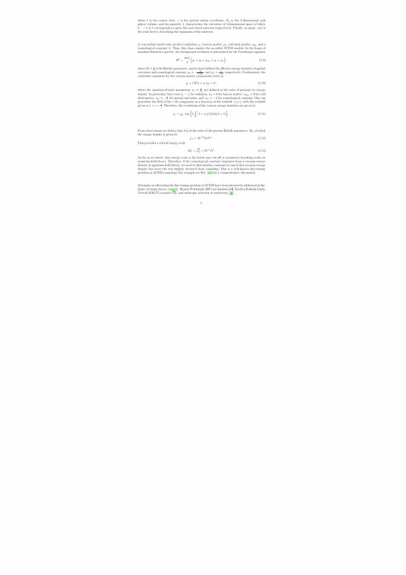
the exponential, as well as other simple potential forms, belong to quintom-A type, which isrealized easily. However, if one desires to construct a specific model of quintom-B type then hehas to use more sophisticated or fine-tuned potentials, or to add more degrees of freedom [104].Alternatively he can include higher derivative terms (see for example [87]), or add suitably con-structed interactive terms which lead to a transition from phantom-to-quintessence domination(see [82]). Generally speaking, both quintom-A and quintom-B types could be consistent withcurrent observational data.
One question arises naturally: is there a cosmic duality between these two quintom types? Dual-ities in field and string theory have been widely studied, predicting many interesting phenomena[160]. The authors of [161,162] have considered a possible transformation with the Hubble pa-rameter and they have studied the relevant issues with the cosmic duality [163,164]. Specifically,
in [165] a link between standard cosmology with quintessence matter and contracting cosmologywith phantom, has been shown. Later on this duality was generalized into more complicated DEmodels, where it has been shown to exist too [166,167,168,169,170,171]. In [172,173] the authorshave studied this cosmic duality and its connection to the fates of the universe, while in [174] theauthor has also discussed the possibility of realizing the aforementioned duality in braneworldcosmological paradigm. A common feature of these studies is that the EoS parameter does notcross −1. Therefore, it would be interesting to study the implications of this cosmic duality inquintom models of DE, and in particular between quintom-A and quintom-B types.
We consider the simple quintom model constructed in 4.1. Following [105,165] we can construct
24

8/3/2019 Yi-Fu Cai et al- Quintom Cosmology: theoretical implications and observations
http://slidepdf.com/reader/full/yi-fu-cai-et-al-quintom-cosmology-theoretical-implications-and-observations 28/105
a form-invariant transformation by defining a group of new quantities H , ρ, ¯ p and w which keepEinstein equations invariant:
ρ = ρ (ρDE ) , (4.40)
H = −
ρρDE
1
2
H . (4.41)
Under this transformation, we obtain the corresponding changes for the pressure pDE and theEoS wDE ,
¯ p = −ρ −
ρDE
ρ
12
(ρDE + pDE )dρ
dρDE , (4.42)
w = −1 − ρDE
ρ
32 dρ
dρDE (1 + wDE ) . (4.43)
From relations (4.42) and (4.43) one can see that for a positive dρdρDE
, one would be able toestablish a connection between the quintom-A and quintom-B types. Assuming without loss of generality, and as an example for a detailed discussion, that ρ = ρDE in (4.42) and (4.43), wecan obtain the dual transformation:
H = −H , (4.44)
¯ p =
−2ρDE
− pDE , (4.45)
w = −2 − wDE . (4.46)
Consequently, using the canonical and phantom energy density definitions (4.6) and (4.7), wecan extract the dual form of the (quintom) DE Lagrangian:
L =1
2∂ µσ∂ µσ − 1
2∂ µφ∂ µφ − δL1(φ) − δL2(σ) , (4.47)
where δL1 and δL2 are
δL1 = V φ(φ) + φ2 , (4.48)
δL2 = V σ(σ) − σ2 . (4.49)
Therefore, we can easily see that if the original Lagrangian is a quintom-A type then the dual oneis a quintom-B type, and vice versa. Thus, under this duality one expects a general connectionamongst different fates of the universe, and it might be possible that the early universe is linkedto its subsequent epochs.
For a specific discussion let us impose a special form for the potentials [105]:
25

8/3/2019 Yi-Fu Cai et al- Quintom Cosmology: theoretical implications and observations
http://slidepdf.com/reader/full/yi-fu-cai-et-al-quintom-cosmology-theoretical-implications-and-observations 29/105
V φ(φ) ∝−3√
2φ + 2e−√
2φ , (4.50)
V σ(σ) ∝ 3
2σ2 + 4σ . (4.51)
Solving explicitly the cosmological equation (4.2), (4.3), (4.8), (4.9), neglecting the matter density,
we study the two periods of the universe evolution. For early times where |t| ≪ 1 (in Planckmass units), we choose the initial conditions by fixing φ → −∞ and σ → 0. With these initialconditions we can see that the dominant component in DE density is the exponential term of V φ(φ) in (4.50), and thus the contribution from the phantom potential in (4.51) and the linearpart of quintessence potential in (4.50) can be neglected. Therefore, the universe behaves likebeing dominated by the quintessence component φ and it evolves following the approximateanalytical solution [105]:
φ ∼√
2 ln |t| , σ ∼ 1
2t2 , H ∼ 1
t. (4.52)
Thus, we see that the scale factor in this period would variate with respect to time as: a ∝ ±t,in which the signal is determined by the positive definite form of the scale factor. Therefore,the scale factor here corresponds to the Big Bang or Big Crunch of quintessence-dominanateduniverse.
The dual form of the solution above is a description of a universe dominated by a phantomcomponent with a Lagrangian given by (4.47) and
δL1 + δL2 = φ2 − σ2 + V φ(φ) + V σ(σ) ∝−3√2φ + 4e−
√ 2φ + 2σ + 32
σ2
. (4.53)
In addition, the dual Hubble parameter is of the form H ∼ −1t
and for the scale factor weacquire a ∝ ±1
t. Accordingly, the scale factor of the dual form is tending towards infinity in the
beginning or the end of universe. From what we have investigated so far, we can see that, forthe positive branch there is a duality between an expanding universe with initial singularity att = 0+ and a contracting one that begins with an infinite scale factor at t = 0+. However, forthe negative branch there is a duality between a contracting universe ending in a big crunch att = 0− and an expanding one that ends in a final Big Rip at t = 0−. The latter is dominated by aphantom component. Besides, in general, under phantom domination the contracting solution is
not stable, because the phantom universe will evolve into Big Rip or Big Sudden or will expandforever approaching to a de Sitter solution, and thus it will not be able to stay in the contractingphase forever [175,176]. This problem, however, can be avoided in quintom cosmology since inthe dual universe with quintom-B DE the increase of kinetic energy of phantom during thecontraction can be set off by that of quintessence at late time.
For times where |t| ≫ 1, the phantom component in the first quintom model will dominate andthe universe will expand. For the specific potentials (4.50) and (4.51) the mass term in V σ(σ)will gradually play an important role in the evolution of DE. Proceeding as above we obtain:
26

8/3/2019 Yi-Fu Cai et al- Quintom Cosmology: theoretical implications and observations
http://slidepdf.com/reader/full/yi-fu-cai-et-al-quintom-cosmology-theoretical-implications-and-observations 30/105
φ ∼√
2 ln |t| , σ ∼√
2t , H ∼ t, (4.54)
where we note that the scale factor is a ∝ exp( t2
2). Consequently, the scale factor would increase
towards infinity rapidly for the positive branch, while it would start from infinity for the negativebranch. In this case, the transformed Lagrangian is (4.47) with
δL1 + δL2 ∝−3
√2φ + 4e−
√ 2φ + 4σ +
3
2σ2 − 2
. (4.55)
The universe is evolving with a Hubble parameter H ∼ −t and a scale factor a ∝ exp(− t2
2 ), whichis close to singularity related to the origin and the fate of universe. Finally, the component whichdominates the evolution of the universe is σ, that is the scalar field resembling quintessence in(4.47). Consequently we conclude that, for the positive branch, there is a dual relation between anexpanding universe with a fate of expanding for ever with t → +∞ and a contracting universewith a destiny of shrinking for ever with t → +∞. Meanwhile, for the negative one, there is
a duality connecting a contracting universe starting from near infinity with t → −∞ and anexpanding universe originating from infinity with t → −∞.
Having presented the analytical arguments for the duality between quintom A and quintomB types, we proceed to numerical investigation. In Fig.9 we depict the evolution of the EoSparameter of the quintom model and its dual. One can see from this figure that under theframework of the duality studied above, the EoS of the quintom model and its dual are symmetricaround w = −1. Accordingly, in this case quintom A is dual to quintom B rigorously, whichsupports our analytical arguments above.
- 6 0 - 4 0 - 2 0 0 2 0 4 0
- 1 . 0 2
- 1 . 0 1
- 1 . 0 0
- 0 . 9 9
- 0 . 9 8
w
l n a
Q u i n t o m A
Q u i n t o m B
Fig. 9. (Color Online)Evolution of EoS parameter w of the quintom model and its dual as a function
of the scale factor ln a for V = −3√
2M 3φ + 2M 4e−√2φM + 3
2M 2σ2 + 4M 3σ and M is the Planck mass.From Ref. [ 105 ].
27

8/3/2019 Yi-Fu Cai et al- Quintom Cosmology: theoretical implications and observations
http://slidepdf.com/reader/full/yi-fu-cai-et-al-quintom-cosmology-theoretical-implications-and-observations 31/105
In Fig.10 we assume the potentials V φ(φ) and V σ(σ) to be exponentials and one can see that theEoS parameter for quintom A approaches to a fixed value which corresponds to the attractorsolution of this type of model [82]. Through the duality we can see that there exists a corre-sponding attractor of the quintom B model dual to the former one. finally, in Fig.11, we provideanother example for the duality.
- 6 0 - 4 0 - 2 0 0 2 0 4 0 6 0 8 0
- 1 . 0 6
- 1 . 0 4
- 1 . 0 2
- 1 . 0 0
- 0 . 9 8
- 0 . 9 6
- 0 . 9 4
w
l n a
Q u i n t o m A
Q u i n t o m B
Fig. 10. (Color Online)Evolution of EoS parameter w of the quintom model and its dual as a function
of the scale factor ln a for V = V 0(e−φ
M + e−2σM ) and M is the planck mass. From Ref. [ 105] .
In summary, we have shown that the quintom model has its dual partner, specifically the quintomA model is dual to the quintom B one, while the cosmological equations are form-invariant. Thesetwo models describe two different behaviors of the universe evolution with one in the expandingphase and the other in the contracting one, depending on the imposed initial conditions. Thecosmic duality, which connects the two totally different scenarios of universe evolution, preservesthe energy density of the universe unchanged but it transforms the Hubble parameter.
5 Perturbation theory and current observational constraints
In this section we investigate the perturbations of quintom DE scenario and the effects of theseperturbations on current observations. As proved in Section 3, it is forbidden for a single fluid orscalar field to realize a quintom scenario in conventional cases, and thus one is led to add extradegrees of freedom. Therefore, it is important to check the consistency of this extension at theclassical level and in particular to analyze the behavior of perturbations when the EoS crossesthe cosmological constant boundary [25].
28

8/3/2019 Yi-Fu Cai et al- Quintom Cosmology: theoretical implications and observations
http://slidepdf.com/reader/full/yi-fu-cai-et-al-quintom-cosmology-theoretical-implications-and-observations 32/105
- 5 0 0 5 0 1 0 0 1 5 0
- 1 . 0 0 4
- 1 . 0 0 2
- 1 . 0 0 0
- 0 . 9 9 8
- 0 . 9 9 6
w
l n a
Q u i n t o m A
Q u i n t o m B
Fig. 11. (Color Online)Evolution of EoS parameter w of the quintom model and its dual as a function of the scale factor ln a for V = m1
2φ2 + m22σ2 where m1 corresponds to the quintessence component
mass and m2 the phantom component mass. From Ref. [105 ].
5.1 Analysis of perturbations in quintom cosmology
As we have argued above, the quintom scenario needs extra degrees of freedom to the conventionalmodels of a single scalar field, and the simplest realization of the quintom is a model with two
scalar fields or two “effective” scalar fields in the case of higher-derivative operators. In thefollowing discussions on quintom perturbations we will restrict ourselves to the double-field modelof quintom with the lagrangian
L = LQ + LP , (5.1)
where
LQ =1
2∂ µφ1∂ µφ1 − V 1(φ1) (5.2)
describes the quintessence component, and
LP = −1
2∂ µφ2∂ µφ2 − V 2(φ2) (5.3)
for the phantom component. The background equations of motion for the two scalar fields φi(i =1, 2) are
φi + 2Hφi ± a2 ∂V i∂φi
= 0 , (5.4)
where the positive sign is for the quintessence and the minus sign for the phantom. In generalthere will be couplings between the two scalar fields, but for simplicity we neglect them.
For a complete perturbation study, both the fluctuations of the fields, as well as those of themetric, need to be considered. In the conformal Newtonian gauge the perturbed metric is given
29

8/3/2019 Yi-Fu Cai et al- Quintom Cosmology: theoretical implications and observations
http://slidepdf.com/reader/full/yi-fu-cai-et-al-quintom-cosmology-theoretical-implications-and-observations 33/105
byds2 = a2(τ )[(1 + 2Ψ)dτ 2 − (1 − 2Φ)dxidxi] . (5.5)
Using the notations of [83], the perturbation equations satisfied by each component of the two-field quintom model read:
δi = −(1 + wi)(θi − 3Φ) − 3H
δP iδρi
− wi
δi , (5.6)
θi = −H(1 − 3wi) θi − wi
1 + wiθi + k2
δP i/δρi
1 + wiδi − σi + Ψ
, (5.7)
where
θi = (k2/φi)δφi , σi = 0 , wi =P iρi
, (5.8)
and
δP i = δρi − 2V ′i δφi = δρi +ρiθi
k2
3H(1 − w2
i ) + wi
. (5.9)
Combining Eqs. (5.6), (5.7) and (5.9), we have
θi = 2Hθi +k2
1 + wiδi + k2Ψ , (5.10)
δi = −(1 + wi)(θi − 3Φ) − 3H(1 − wi)δi − 3H wi + 3H(1 − w2
i )k2
θi . (5.11)
Since the simple two-field quintom model is essentially a combination of a quintessence anda phantom field, one obtains the perturbation equations of quintom by combining the aboveequations. The corresponding variables for the quintom system are
wquintom =
i P ii ρi
, (5.12)
δquintom = i ρiδii ρi
, (5.13)
θquintom =
i(ρi + pi)θi
i(ρi + P i). (5.14)
Note that for the quintessence component, −1 ≤ w1 ≤ 1, while for the phantom component,w2 ≤ −1.
The two-field quintom model is characterized by the potentials V i. Let us consider V i(φi) =12
m2i φ2
i . In general the perturbations of φi today stem from two origins, the adiabatic and the
isocurvature modes. If we use the gauge invariant variable ζ i = −Φ − H δρiρi
instead of δi, and the
30

8/3/2019 Yi-Fu Cai et al- Quintom Cosmology: theoretical implications and observations
http://slidepdf.com/reader/full/yi-fu-cai-et-al-quintom-cosmology-theoretical-implications-and-observations 34/105
relation Φ = Ψ in the universe without anisotropic stress, the equations (5.11) and (5.10) can berewritten as,
ζ i =
−θi
3 −C i ζ i + Φ +
Hk2
θi , (5.15)
θi = 2Hθi + k2(3ζ i + 4Φ) , (5.16)
where
C i =wi
1 + wi
+ 3H(1 − wi) = ∂ 0[ln(a6|ρi + pi|)] . (5.17)
ζ α is the curvature perturbation on the uniform-density hypersurfaces for the α-component in theuniverse [177]. Usually, the isocurvature perturbations of φi are characterized by the differencesbetween the curvature perturbation of the uniform-φi-density hypersurfaces and that of theuniform-radiation-density hypersurfaces,
S ir ≡ 3(ζ i − ζ r) , (5.18)
where the subscript r represents radiation. We assume there are no matter isocurvature pertur-bations and thus ζ M = ζ r. Eliminating ζ i from equations (5.15) and (5.16), we obtain a secondorder equation for θi, namely
¨θi + (C i − 2H)
˙θi + (C iH − 2
˙H + k
2
)θi = k
2
(4˙
Φ + C iΦ) . (5.19)
This is an inhomogeneous differential equation and its general solution is the sum of the generalsolution of its homogeneous part and a special integration. In the following, we will show that thespecial integration corresponds to the adiabatic perturbation. Before the era of DE domination,the universe is dominated by some background fluids, for instance, the radiation or the matter.The perturbation equations of the background fluid are,
ζ f = −θf /3 ,
θf =
−H(1
−3wf )θf + k2[3wf ζ f + (1 + 3wf )Φ] . (5.20)
From the Poisson equation
− k2
H2Φ =
9
2
α
Ωα(1 + wα)
ζ α + Φ +Hk2
θα
≃ 9
2(1 + wf )
ζ f + Φ +
Hk2
θf
, (5.21)
on large scales we approximately acquire:
31

8/3/2019 Yi-Fu Cai et al- Quintom Cosmology: theoretical implications and observations
http://slidepdf.com/reader/full/yi-fu-cai-et-al-quintom-cosmology-theoretical-implications-and-observations 35/105
Φ ≃ −ζ f − Hk2
θf . (5.22)
Combining these equations with H = 2/[(1+3wf )τ ], we obtain (note numerically θf ∼ O(k2)ζ f )
ζ f = − 5 + 3wf
3(1 + wf )Φ = const. ,
θf =k2(1 + 3wf )
3(1 + wf )Φτ . (5.23)
Thus, we can see from Eq. (5.19) that there is a special solution, which is given approximatelyon large scales by θad
i = θf , and from Eq. (5.16) we have ζ adi = ζ f . This indicates that the
special integration of (5.19) corresponds to the adiabatic perturbation. Hence, concerning theisocurvature perturbations of φi, we can consider only the solution of the homogeneous part of (5.19):
θi + (C i − 2H)θi + (C iH − 2H + k2)θi = 0 . (5.24)
These solutions are represented by θisoi and ζ iso
i and the relation between them is
ζ isoi =
θisoi − 2Hθiso
i
3k2. (5.25)
Since the general solution of ζ i is ζ i = ζ adi + ζ iso
i = ζ r + ζ isoi , the isocurvature perturbations are
simply S ir = 3ζ isoi .
In order to solve Eq. (5.24) we need to know the forms of C i and H as functions of time τ .For this purpose, we solve the background equations (5.4). In radiation dominated period, a =Aτ , H = 1/τ and we have
φ1 = τ −1/2
A1J 1/4(
A
2m1τ 2) + A2J −1/4(
A
2m1τ 2)
, (5.26)
φ2 = τ −1/2
A1I 1/4(
A
2m2τ 2) + A2I −1/4(
A
2m2τ 2)
, (5.27)
respectively, where A, Ai and Ai are constants, J ν (x) is the ν th order Bessel function and I ν (x)is the ν th order modified Bessel function. Usually the masses are small in comparison with theexpansion rate in the early universe mi ≪ H/a, and we can approximate the (modified) Besselfunctions as J ν (x) ∼ xν (c1 + c2x2) and I ν (x) ∼ xν (c1 + c2x2). We note that J −1/4 and I −1/4 aredivergent when x → 0. Given these arguments one can see that this requires large initial valuesof φi and φi if A2 and A2 are not vanished.
If we choose small initial values, which is the natural choice if the DE fields are assumed to surviveafter inflation, only A1 and A1 modes exist, so φi will be proportional to τ 3 in the leading order.
32

8/3/2019 Yi-Fu Cai et al- Quintom Cosmology: theoretical implications and observations
http://slidepdf.com/reader/full/yi-fu-cai-et-al-quintom-cosmology-theoretical-implications-and-observations 36/105
Thus, the parameters C i in equation (5.17) will be C i = 10/τ (we have used |ρi + pi| = φ2i /a2).
Therefore, we obtain the solution of Eq. (5.24) as
θisoi = τ −4Di1 cos(kτ ) + Di2 sin(kτ ) . (5.28)
That is, θisoi presents an oscillatory behavior, with an amplitude damping with the expansion of
the universe. The isocurvature perturbations ζ isoi decrease rapidly.
On the other hand, if we choose large initial values for φi and φi, A2 and A2 modes are present,φi will be proportional to τ −2 in the leading order and C i = 0. Thus, the solution of (5.24) is
θisoi = τ
Di1 cos(kτ ) + Di2 sin(kτ )
. (5.29)
Therefore, θisoi will oscillate with an increasing amplitude, so ζ iso
i remains constant on large scales.
Similarly, during matter dominated era, a = Bτ 2, H = 2/τ , and the solutions for the fields φi
read:
φ1 = τ −3
B1 sin(
B
3m1τ 3) + B2 cos(
B
3m1τ 3)
, (5.30)
φ2 = τ −3
B1 sinh(
B
3m2τ 3) + B2 cosh(
B
3m2τ 3)
. (5.31)
We acquire the same conclusions as those reached by the aforementioned analysis for the radiationdominated era. If we choose small initial values at the beginning of the matter domination wefind that the isocurvature perturbations in φi decrease with time. On the contrary, for largeinitial values the isocurvature perturbations remain constant at large scales. This conclusion isexpectable. In the case of large initial velocity, the energy density in the scalar field is dominatedby the kinetic term and it behaves like the fluid with w = 1. The isocurvature perturbation insuch a fluid remains constant on large scales. In the opposite case, however, the energy densityin the scalar field will be dominated by the potential energy due to the slow rolling. It behaveslike a cosmological constant, and there are only tiny isocurvature perturbations in it.
In summary, we have seen that the isocurvature perturbations in quintessence-like or phantom-like field with quadratic potential, decrease or remain constant on large scales depending onthe initial velocities. In this sense the isocurvature perturbations are stable on large scales.The amplitude of these perturbations will be proportional to the value of Hubble rate evaluatedduring the period of inflation H inf , if their quantum origins are from inflation. For a large H inf theisocurvature DE perturbations may be non-negligible and will contribute to the observed CMBanisotropy [178,179]. In the cases discussed here, however, these isocurvature perturbations arenegligible. Firstly, large initial velocities are not possible if these fields survive after inflation asmentioned above. Secondly, even if the initial velocities are large at the beginning of the radiationdomination, they will be reduced to a small value due to the small masses and the damping
33

8/3/2019 Yi-Fu Cai et al- Quintom Cosmology: theoretical implications and observations
http://slidepdf.com/reader/full/yi-fu-cai-et-al-quintom-cosmology-theoretical-implications-and-observations 37/105
effect of Hubble expansion. In general the contributions of DE isocurvature perturbations arenot very large [180], and here for simplicity we have assumed that H inf is small enough and thusthe isocurvature contributions are negligible. Therefore, in the next subsection we focus on theeffects of the adiabatic perturbations of the quintom model with two scalars fields.
5.2 Signatures of perturbations in quintom DE
Based on perturbation equations (5.13) and (5.14), we modify the code of CAMB [181] and westudy preliminarily in this subsection the quintom observational signatures. For simplicity weimpose a flat geometry as a background, although this is not necessary. Moreover, we assume thefiducial background parameters to be Ωb = 0.042, ΩDM = 0.231, ΩDE = 0.727, where b stands forbaryons, DM for dark matter and DE for dark energy, while today’s Hubble constant is fixed atH 0 = 69.255 km/s Mpc−2. We will calculate the effects of perturbed quintom on CMB and LSS.
In the two-field quintom model there are two parameters, namely the quintessence and phantommasses. When the quintessence mass is larger than the Hubble parameter, the field starts tooscillate and consequently one obtains an oscillating quintom. In the numerical analysis we fixthe phantom mass to be mP ∼ 4 × 10−61M p, and we vary the quintessence mass with thetypical values being mQ = 2 × 10−61M p and 8 × 10−61M p respectively. In Fig. 12 we depictthe equation-of-state parameters as a function of the scale factor, for the aforementioned twoparameter-sets, and additionally their corresponding effects on observations. We clearly observethe quintom oscillating behavior as the mass of quintessence component increases. After reachingthe w = −1 pivot for several times, w crosses −1 consequently with the phantom-componentdomination in dark energy. As a result, the quintom fields modify the metric perturbations
δg00 = 2a2
Ψ, δgii = 2a2
Φδij, and consequently they contribute to the late-time Integrated Sachs-Wolfe (ISW) effect. The ISW effect is an integrant of Φ+Ψ over conformal time and wavenumberk. The above two specific quintom models yield quite different evolving Φ + Ψ as shown in theright graph of Fig.12, where the scale is k ∼ 10−3 Mpc−1. As we can see, the late time ISWeffects differ significantly when DE perturbations are taken into account (solid lines) or not(dashed lines).
ISW effects play an important role on large angular scales of CMB and on the matter powerspectrum of LSS. For a constant EoS of phantom the authors of [ 182] have shown that the lowmultipoles of CMB will be significantly enhanced when DE perturbations are neglected. On theother hand, for a matter-like scalar field where the EoS is around zero, perturbations will also
play an important role on the large scales of CMB, as shown in [183]. The results on CMB andLSS reflect the two combined effects of phantom and oscillating quintessence. Note that in theearly studies of quintessence effects on CMB, one usually considers a constant wef f instead
wef f ≡
daΩ(a)w(a) daΩ(a)
, (5.32)
however this is not enough for the study of effects on SNIa, nor for CMB, when the EoS of DE has a very large variation with redshift, such as the model of oscillating quintom consideredabove.
34

8/3/2019 Yi-Fu Cai et al- Quintom Cosmology: theoretical implications and observations
http://slidepdf.com/reader/full/yi-fu-cai-et-al-quintom-cosmology-theoretical-implications-and-observations 38/105
0 . 2 0 . 4 0 . 6 0 . 8 1 . 0
4 1 . 5 0 . 6 7 0 . 2 5 0
0 . 8 4 0 . 9 0 0 . 9 6
1 0 1 0 0 1 0 0 0
1 E - 5 1 E - 4 1 E - 3 0 . 0 1 0 . 1 1
1 0 0 0
1 0 0 0 0
0 . 2 0 . 4 0 . 6 0 . 8 1 . 0
= 1 x 1 0
= 4 x 1 0
w
Q
m
+
C
T
T
M u l t i p o l e l
W a v e n u m b e r k ( h M p c
P
M
s o l i d : w i t h p e r t u r b a t i o n
d a s h e d : w i t h o u t p e r t u r b a t i o n
Fig. 12. (Color online) Effects of the two-field oscillating quintom on the observables. The mass of thephantom field is fixed at 4 × 10−61M p and the mass of the quintessence field are 2 × 10−61M p (thicker line) and 8 × 10−61M p (thinner line) respectively. The upper right graph il lustrates the evolution of the metric perturbations Φ + Ψ of the two models, with (solid lines) and without (dashed lines) DE perturbations. The scale is k ∼ 10−3 Mpc−1. The lower left graph shows the CMB effects and the lower right graph delineates the effects on the matter power spectrum, with (solid lines) and without (dashed lines) DE perturbations. From Ref. [25] .
To analyze the oscillating quintom-model under the current observations, we perform a pre-liminary fitting to the first year WMAP TT and the TE temperature–polarization cross-powerspectrum, as well as the recently released 157 “Gold” SNIa data [28]. Following Refs. [184,185] inall the fittings below we fix τ = 0.17, ΩM h
2 = 0.135 and Ωbh2 = 0.022, setting the spectral indexas nS = 0.95, and using the amplitude of the primordial spectrum as a continuous parameter. Inthe fittings of oscillating quintom we have fixed the phantom-mass to be mP ∼ 1.2 × 10−61M p.Fig.13 delineates 3σ WMAP and SNIa constraints on the two-field quintom model, and in ad-dition it shows the corresponding best fit values. In the left graph of Fig.13 we present theseparate WMAP and SNIa constraints. The green (shaded) area marks WMAP constraints onmodels where DE perturbations have been included, while the blue area (contour with solid
35

8/3/2019 Yi-Fu Cai et al- Quintom Cosmology: theoretical implications and observations
http://slidepdf.com/reader/full/yi-fu-cai-et-al-quintom-cosmology-theoretical-implications-and-observations 39/105
Fig. 13. (Color online) 3 σ WMAP and SNIa constraints on two-field quintom model, shown together with the best fit values. mQ and mP denote the quintessence and phantom mass respectively. We have fixed mP ∼ 1.2 × 10−61M p and we have varied the value of mQ. Left graph: separate WMAP and SNIa constraints. The green (shaded) area marks the WMAP constraints on models where DE perturbationshave been included, while the blue area (contour with solid lines) corresponds to the case where DE perturbations have not been taken into account. Right graph: combined WMAP and SNIa constraintson the two-field quintom model with perturbations (green/shaded region) and without perturbations (red region/contour with solid lines). From Ref. [25] .
lines) is the corresponding area without DE perturbations. The perturbations of DE have no
effects on the geometric constraint of SNIa. The right graph shows the combined WMAP andSNIa constraints on the two-field quintom model with perturbations (green/shaded region) andwithout perturbations (red region/contour with solid lines). We conclude that the confidenceregions indeed present a large difference, if the DE perturbations have been taken into accountor not.
So far we have investigated the imprints of oscillating quintom on CMB and LSS. Now we consideranother example, in which w crosses −1 smoothly without oscillation. It is interesting to studythe effects of this type of quintom model, with its effective EoS defined in ( 5.32) exactly equal to−1, on CMB and matter power-spectrum. This investigation will help to distinguish the quintom
36

8/3/2019 Yi-Fu Cai et al- Quintom Cosmology: theoretical implications and observations
http://slidepdf.com/reader/full/yi-fu-cai-et-al-quintom-cosmology-theoretical-implications-and-observations 40/105
3 0 0 0
6 0 0 0
1 1 0 1 0 0 1 0 0 0
- 8 - 6 - 4 - 2 0
- 3 . 5
- 3 . 0
- 2 . 5
- 2 . 0
- 1 . 5
- 1 . 0
- 0 . 5
1 2 0 0
2 3 4 5
1 E - 3 0 . 0 1 0 . 1 1
0 . 0 0 . 2 0 . 4 0 . 6 0 . 8 1 . 0
1 s t y e a r W M A P d a t a
l
(
l
+
1
)
C
T
T
l
/
2
2
(
l
+
1
)
C
T
E
l
/
2
2
M u l t i p o l e l
w
- 0 . 1 4 4
C r o s s i n g p o i n t : z = 0 . 1 5
Q u i n t e s s e n c e
P h a n t o m
Q u i n t o m w i t h w
l
(
l
+
1
)
C
T
T
l
/
2
2
G
w
F
l n a
p e r t u r b a t e d Q u i n t o m w i t h w = - 1
u n p e r t u r b a t e d Q u i n t o m w i t h w = - 1
C D M
C D M
Q u i n t o m w i t h w
Fig. 14. (Color online) Comparison of the effects of the two-field quintom model with wef f = −1 and of the simple cosmological constant, in CMB (WMAP), the metric perturbations Φ + Ψ (the scale isk ∼ 10−3 Mpc−1) and the linear growth factor. The binned error bars in the upper right graph areWMAP TT and TE data [ 186,187 ]. From Ref. [ 25] .
model from the cosmological constant. We have realized such a quintom model in the lower rightgraph of Fig. 14, which can be easily given in the two-field model with lighter quintessence mass.
In this example we have set mQ ∼ 5.2 × 10−62
M p and mP ∼ 1.2 × 10−61
M p. Additionally, weassume that there is no initial kinetic energy. The initial value of the quintessence component isset to φ1i = 0.045M p, while for the phantom part we impose φ2i = 1.32 × 10⁻³M p. We find thatthe EOS of quintom crosses −1 at z ∼ 0.15, which is consistent with the latest SNIa results.
The quintom scenario, which is mildly favored by current SNIa data, needs to be confronted withother observations in the framework of concordance cosmology. Since SNIa offer the only directdetection of DE, this model is the most promising to be distinguished from the cosmologicalconstant and other dynamical DE models which do not get across −1, by future SNIa projectson the low redshift (for illustrations see e.g. [20]). This is also the case for quintom scenario in the
37

8/3/2019 Yi-Fu Cai et al- Quintom Cosmology: theoretical implications and observations
http://slidepdf.com/reader/full/yi-fu-cai-et-al-quintom-cosmology-theoretical-implications-and-observations 41/105
full parameter space: it can be most directly tested in low redshift Type Ia supernova surveys.In the upper left graph of Fig. 14 we delineate the different ISW effects among the cosmologicalconstant (red/light solid) and the quintom model which exhibits wef f = −1, with (blue/darksolid) and without (blue dashed) perturbations. Similarly to the previous oscillating case, thedifference is big when switching off quintom perturbations and much smaller when including the
perturbations. In the upper right graph we find that the quintom model cannot be distinguishedfrom a cosmological constant in light of WMAP. The two models give almost exactly the sameresults in CMB TT and TE power-spectra when including the perturbations. We deduce thatthe difference in CMB is hardly distinguishable even by cosmic variance.
So far we have seen that CMB observations cannot distinguish between a quintom model withwef f = −1 and a cosmological constant. Thus, in order to acquire distinctive signatures, we haveto rely on other observations. To achieve that we need to consider the physical observables whichcan be affected by the evolving w sensitively. In comparison with the cosmological constant,such a quintom model exhibits a different evolution of the universe’s expansion history, and inparticular it gives rise to a different epoch of matter-radiation equality. The Hubble expansion
rate H isH ≡ a
a2= H 0[ΩM a
−3 + Ωra−4 + X ]1/2, (5.33)
where X , the energy density ratio of DE between the early times and today, is quite differentbetween the quintom-CDM and ΛCDM. In the ΛCDM scenario X is simply a constant, while ingeneral for DE models with varying energy density or EoS,
X = ΩDE a−3e−3
w(a)d ln a . (5.34)
The two models will give different Hubble expansion rates. This is also the case between thequintom model with wef f = −1 in the left graph of Fig. 14 and a cosmological constant.
Finally, we mention that different H leads directly to different behaviors of the growth factor. Inparticular, according to the linear perturbation theory all Fourier modes of the matter densityperturbations grow at the same rate, that is the matter density perturbations are independentof k:
δk + Hδk − 4πGa2ρMδk = 0 . (5.35)
The growth factor D1(a) characterizes the growth of the matter density perturbations: D1(a) =δk(a)/δk(a = 1) and it is normalized to unity today. In the matter-dominated epoch we haveD1(a) = a. Analytically D1(a) is often approximated by the Meszaros equation [188] 2 :
D1(a) =
5ΩM H (a)
2H 0 a0
da′
(a′H (a′)/H 0)3 . (5.36)
Therefore, we can easily observe the difference between the quintom and cosmological constantscenarios, due to the different Hubble expansion rates. More strictly one needs to solve Eq.(5.35)numerically. In the lower left graph of Fig. 14 we show the difference of D1(a) between the
2 One should notice that the Meszaros equation is an exact solution to the differential equation for thelinear-theory growth factor only when dark energy is a cosmological constant or it is absent. However,it is still a good approximation in the case of dynamical dark energy models on small length scales of the universe, as in the analysis of Section 3.1 of Ref. [189].
38

8/3/2019 Yi-Fu Cai et al- Quintom Cosmology: theoretical implications and observations
http://slidepdf.com/reader/full/yi-fu-cai-et-al-quintom-cosmology-theoretical-implications-and-observations 42/105
quintom with wef f = −1 and the cosmological constant. The difference in the linear growthfunction is considerably large in the late-time evolution, and thus possibly distinguishable infuture LSS surveys and in weak gravitational lensing (WGL) observations. WGL has emergedwith a direct mapping of cosmic structures and it has been recently shown that the methodof cosmic magnification tomography can be extremely efficient [190,191,192], which leaves a
promising future for breaking the degeneracy between quintom and a cosmological constant.
6 Quintom models with higher derivative terms
As we demonstrated previously, we usually need to introduce new degrees of freedom into anormal lagrangian in order to obtain a viable quintom scenario. One approach is to construct a
double-field quintom model introduced in Section IV. In this section we provide an alternativepossibility of introducing extra degrees of freedom for the realization of the transition betweenquintessence phase and phantom phase [193]. This model is originally proposed by Lee and Wickto address on hierarchy problem in particle physics in the 70’s [194,195], and recently applied in[87] involving higher derivative operators in the Lagrangian.
6.1 Lee-Wick model
In this subsection we present a single field model with the inclusion of higher derivatives, following[87]. We consider a Lagrangian of the form
L = L
φ,X, (2φ)(2φ), (∇µ∇ν φ)(∇µ∇ν φ)
, (6.1)
where X = 1/2∇µφ∇µφ and 2 ≡ ∇µ∇µ is the d’Alembertian operator. We mention that thismodel is just an effective theory and one assumes that the operators associated with the higherderivatives can be derived from some fundamental theories, for instance due to the quantumcorrections or the non-local physics in string theory [196,197,198]. Additionally, with the inclusionof higher derivative terms to the Einstein gravity, the theory is shown to be renormalizable[199]. Finally, higher derivative operators have been shown to be capable of stabilizing the linearfluctuations in the scenario of “ghost condensation” [200,201,202,203,204,205].
We consider the simple model with
L = −1
2∇µφ∇µφ +
c
2M 2(2φ)2 − V (φ) , (6.2)
where M is a constant with mass dimension and c is a dimensionless constant. The energy-momentum tensor reads [87]:
39

8/3/2019 Yi-Fu Cai et al- Quintom Cosmology: theoretical implications and observations
http://slidepdf.com/reader/full/yi-fu-cai-et-al-quintom-cosmology-theoretical-implications-and-observations 43/105
T µν = gµν
1
2∇ρφ∇ρφ +
c
2M 2(2φ)2 +
c
M 2∇ρφ∇ρ(2φ) + V
− ∇µφ∇ν φ −
− c
M 2
∇ν φ∇µ(2φ) + ∇µφ∇ν (2φ)
, (6.3)
and the equation of motion is given by
− 2φ − c
M 22
2φ +dV
dφ= 0 . (6.4)
However, the energy-momentum tensor (6.3) can be rewritten as
T µν = ∇µχ∇ν χ − ∇µψ∇ν ψ +1
2
∇ρψ∇ρψ − ∇ρχ∇ρχ + 2V (ψ − χ) +
M 2
cχ2
gµν , (6.5)
where χ and ψ are defined by
χ =c
M 22φ , ψ = φ + χ . (6.6)
It is not difficult to see that the energy-momentum tensor (6.5) can be derived from the followingLagrangian
L = −1
2∇µψ∇µψ +
1
2∇µχ∇µχ − V (ψ − χ) − M 2
2cχ2 , (6.7)
with ψ and χ being two independent fields. The variations of the Lagrangian (6.7), with respectto the fields ψ and χ respectively, give rise to the equations of motions
2ψ − V ′ = 0 , (6.8)
2χ +M 2
cχ − V ′ = 0 , (6.9)
where the prime denotes the derivative with respect to ψ − χ.
When one imposes ψ = φ + χ in (6.7) and (6.8), he recovers the equation of motion (6.4) of the single field model and the transformation equation (6.6). Thus, one can see that the singlefield model (6.2) is equivalent to the one with two fields (6.7), where one is the canonical scalarfield χ and the other is the phantom field ψ. Therefore, assuming that χ dominates the DEsector in the early time, the EoS parameter will be larger than −1, but when the phantommode becomes dominant the EoS parameter will become less than −1, crossing the cosmologicalconstant boundary at an intermediate redshift.
In general the potential term V (ψ − χ) (equivalently V (φ) in our single field model) shouldinclude interactions between the two fields ψ and χ. However, for some specific choices of the
40
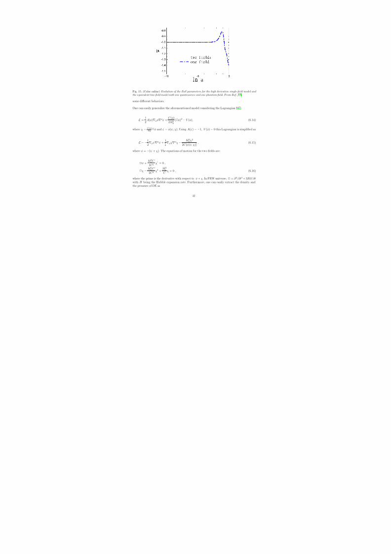
8/3/2019 Yi-Fu Cai et al- Quintom Cosmology: theoretical implications and observations
http://slidepdf.com/reader/full/yi-fu-cai-et-al-quintom-cosmology-theoretical-implications-and-observations 44/105
potential V these two modes could decouple. As an example we consider V = (1/2)m2φ2. Thenthe Lagrangian (6.7) can be “diagonalized” as:
L=
1
2∇µφ1
∇µφ1
−
1
2∇µφ2
∇µφ2
−
1
2
m21φ2
1
−
1
2
m22φ2
2 , (6.10)
through the transformation
ψ
χ
=
−a1 a2
−a2 a1
φ1
φ2
, (6.11)
where
a1 = 12
1 + 4cm
2
M 2−1/4 1 + 4cm
2
M 2 − 1 ,
a2 =1
2
1 +
4cm2
M 2
−1/4
1 +4cm2
M 2+ 1
, (6.12)
and
m21 =
M 2
2c
1 +
4cm2
M 2+ 1
,
m22 =
M 2
2c
1 +4cm2
M 2− 1
. (6.13)
Hence, one can see that the model (6.2) with V = (1/2)m2φ2 is equivalent to the uncoupledsystem (6.10). The two modes φ1 and φ2 evolve independently in the universe. The positivity of the parameter c guarantees the positivity of m2
1 (m22 is always positive as long as 1 + 4cm2
M 2 > 0).In the limit m ≪ M , the masses of the two modes are approximately m1 ≃ M/
√c and m2 ≃ m.
In fact, φ1 and φ2 are the eigenfunctions of the d’Alembertian operator 2, with the eigenvalues−m2
1 and m22 respectively. The solution to the equation of motion (6.4) φ, is decomposed by these
eigenfunctions as φ = (1 + 4cm2
M 2)−1/4(φ1 + φ2). Finally, we mention that the perturbations in the
phantom component φ2 do not present any unphysical instabilities at the classical level. Thus,the model is free from the difficulties of the singularity and the gravitational instabilities of thegeneral k-essence-like scenarios [87].
In Fig. 15 we present the EoS parameter of the single field model as a function of ln a, wherew clearly crosses −1 during evolution. On the same figure it is also depicted the correspondingevolution of EoS parameter of the equivalent two-field model. Indeed, one can see that the twomodels coincide. Therefore, the high derivative single scalar field model of DE presents the −1-crossing, and it is equivalent to the usual two-field quintom paradigm. However, note that whenwe consider the interactions between these two fields in the potential, they may possibly show
41

8/3/2019 Yi-Fu Cai et al- Quintom Cosmology: theoretical implications and observations
http://slidepdf.com/reader/full/yi-fu-cai-et-al-quintom-cosmology-theoretical-implications-and-observations 45/105
- 1 0 - 5 0
- 1 . 5
- 1 . 4
- 1 . 3
- 1 . 2
- 1 . 1
- 1 . 0
- 0 . 9
- 0 . 8
w
l n a
t w o f i e l d s
o n e f i e l d
Fig. 15. (Color online) Evolution of the EoS parameters for the high derivative single-field model and the equivalent two-field model with one quintessence and one phantom field. From Ref. [ 87 ].
some different behaviors.
One can easily generalize the aforementioned model considering the Lagrangian [97]:
L =1
2A(φ)∇µφ∇µφ +
C (φ)
2M 2 p
(2φ)2 − V (φ), (6.14)
where χ = C (φ)M 2p2φ and φ = φ(ψ, χ). Using A(φ) = −1, V (φ) = 0 this Lagrangian is simplified as
L = −1
2∇µψ∇µψ +
1
2∇µχ∇µχ − M 2 p χ2
2C [φ(ψ, χ)], (6.15)
where φ =
−(ψ + χ). The equations of motion for the two fields are:
2ψ +M 2 p C ′
2C 2χ2 = 0 ,
2χ − M 2 p C ′
2C 2χ2 +
M 2 p
C χ = 0 , (6.16)
where the prime is the derivative with respect to ψ + χ. In FRW universe, 2 = ∂ 2/∂t2 + 3H∂/∂twith H being the Hubble expansion rate. Furthermore, one can easily extract the density andthe pressure of DE as
42

8/3/2019 Yi-Fu Cai et al- Quintom Cosmology: theoretical implications and observations
http://slidepdf.com/reader/full/yi-fu-cai-et-al-quintom-cosmology-theoretical-implications-and-observations 46/105
ρ = − ψ2
2+
χ2
2+
M 2 p χ2
2C , (6.17)
p = − ψ2
2+
χ2
2− M 2 p χ2
2C , (6.18)
and thus the EoS parameter writes
w =p
ρ= −1 +
2( χ2 − ψ2)
χ2 − ψ2 +M 2pχ2
C
, (6.19)
where the dot represents the derivative with respect to the cosmic time. Again, χ behaves as acanonical field while ψ as a phantom one. However, in this case they couple to each other throughan effective potential, that is the last term in the right hand side of equation (6.15):
V ef f = M
2
p χ
2
2C [φ(ψ, χ)]. (6.20)
As an example one can consider [97]:
C [φ(ψ, χ)] = C 0
π
2+ arctan
λ(ψ + χ)
M p
. (6.21)
Thus, C is almost constant when |ψ + χ| ≫ 0, and ψ and χ are nearly decoupled at theseregimes, which are dubbed “weak coupling” regimes. By contrast, the two fields couple tightlyin the “strong coupling” regime where |ψ + χ| ∼ 0. In the weak coupling regime, as shown in(6.16), the phantom-like field ψ behaves as a massless scalar field and its energy density −(1/2)ψ2
dilutes as a−6, with a is the scale factor of the universe. The quintessence-like field χ has a mass
term with mχ = M p/
C (ψ + χ). Its behavior is determined by the ratio of mχ/H . If mχ ≪ H , χis slow-rolling and it behaves like a cosmological constant. On the other hand, in cases mχ ≫ H the kinetic term and potential oscillate coherently and their assembly evolves as a−3, just likethat of collisionless dust.
The EoS parameter of such a DE model is depicted in Fig. 16. The initial conditions are chosenin order for the DE to start in the strong coupling regime with χ > 0 at high red-shift. As we
observe, DE is frozen quickly at initial times, and then it becomes significant around redshiftz ∼ 1, and the phantom kinetic term ψ2 becomes larger than the quintessence one χ2. The DEcrosses the phantom divide from above to below. In the future, the system evolves into the weakcoupling regime, ψ2 dilutes quickly and χ gets a large mass. The whole system behaves as coldmatter and its EoS oscillate around the point of w = 0. So, the universe will exit from thephantom phase and end in the state of matter-domination. This result resembles the late-timebehavior of “B-inflation” model [206]. Therefore, the present cosmological scenario differs fromthe simple quintom DE model, since it leads to a double crossing of the phantom divide andit can give a nice exit from phantom phase, in which it stays just for a finite time, avoidingthe realization of a Big Rip [18,129,207,208,209]. In addition, at late times w oscillates with
43

8/3/2019 Yi-Fu Cai et al- Quintom Cosmology: theoretical implications and observations
http://slidepdf.com/reader/full/yi-fu-cai-et-al-quintom-cosmology-theoretical-implications-and-observations 47/105
- 2 0 - 1 0 0 1 0
- 2 0 - 1 8 - 1 6 - 1 4 - 1 2
- 1 . 1
- 1 . 0
- 0 . 9
- 0 . 8
w
w
Fig. 16. (Color online) The EoS parameter w as a function of ln a for C = 6.0 × 10121, λ = 25, and the initial values areψi = −0.052M p, ψi = 1.40 × 10−63M 2 p , χi = 0.050M p, χi = −1.44 × 10−63M 2 p , with ΩDE 0 ≈ 0.73.From Ref. [ 97] .
high frequency around zero, so the universe will end in an accelerated expansion at some time.Finally, note that the quintom model based on higher derivative theory possesses also ghost
degrees of freedom, and thus it could face the problem of quantum instability [51,50]. However,as pointed out in [210], the problem of quantum instability arises because φ and 2φ are quantizedin canonical way independently. In fact, in the present model both of them are determined by φ,and a more appropriate quantization method seems to be possible to avoid the instability [97].
6.2 Quintom DE inspired by string theory
In recent years, there have been active studies on relating quintom scenario with fundamental
physics, and in particular with string theory. In such a context a rolling tachyon field in the worldvolume theory of the open string, stretched between a D-brane and an anti-D-brane or a non-BPSD-brane, plays the role of the scalar field in the quintom model [101,211,212,213,214,215,216,217].The effective action used in the study of tachyon cosmology consists of the standard Einstein-Hilbert action plus an effective action for the tachyon field on unstable D-brane or (D-brane)-(anti-D-brane) system. Such a single-field effective action, to the lowest order in ∇µφ∇µφ aroundthe top of the tachyon potential, can be obtained by the stringy computations for either a D3brane in bosonic theory [218,219] or a non-BPS D3 brane in supersymmetric theory [220] (see also[221] for an application in inflation). What distinguishes the tachyon action from the standardKlein-Gordon form for a scalar field, is that the former is non-standard but it is of the “Dirac-
44

8/3/2019 Yi-Fu Cai et al- Quintom Cosmology: theoretical implications and observations
http://slidepdf.com/reader/full/yi-fu-cai-et-al-quintom-cosmology-theoretical-implications-and-observations 48/105
Born-Infeld” form [222,223,224]. The tachyon potential is derived from string theory itself andthus it has to satisfy some definite properties and requirements, such as to describe the tachyoncondensation.
6.2.1 A model inspired by string theory
In this paragraph we construct a specific quintom model inspired by string theory. One considersan action of the form [110]:
S =
d4x√−g
−V (φ)
1 − α′∇µφ∇µφ + β′φ2φ
, (6.22)
which generalizes the usual“Born-Infeld-type” action, for the effective description of tachyondynamics, by adding a term φ2φ to the usual ∇µφ∇µφ in the square root. The two parametersα′ and β′ in (6.22) can be also made arbitrary when the background flux is turned on [225]. Notethat we have defined α′ = α/M 4 and β′ = β/M 4 with α and β being the dimensionless parameters
respectively, and M an energy scale used to make the “kinetic energy terms” dimensionless.V (φ) is the potential of scalar field φ (e.g., a tachyon) with dimension of [mass]4, with a usualbehavior in general, that is bounded and reaching its minimum asymptotically. Note that, 2 =
1√ −g∂ µ
√−ggµν ∂ ν , and therefore in (6.22) the terms ∇µφ∇µφ and φ2φ both involve two fieldsand two derivatives.
The equation of motion for the scalar field φ reads:
β
22
V φ
f
+ α∇µ
V ∇µφ
f
+ M 4V φf +
βV
2f 2φ = 0 , (6.23)
where f =
1 − α′∇µφ∇µφ + β′φ2φ and V φ = dV/dφ. Following the convention of [87], theenergy-momentum tensor T µν is given by the standard definition δgµνS ≡ − d4x
√ −g2
T µν δgµν ,thus:
T µν = gµν [V (φ)f + ∇ρ(ψ∇ρφ)] +α
M 4V (φ)
f ∇µφ∇ν φ − ∇µψ∇ν φ − ∇ν ψ∇µφ, (6.24)
where ψ ≡ ∂ L∂ 2φ
= − V βφ2M 4f
.
For a flat FRW universe and a homogenous scalar field φ, the equation of motion (6.23) can be
solved equivalently by the following two equations
φ + 3H φ =βV 2φ
4M 4ψ2− M 4
βφ+
α
βφφ2 , (6.25)
ψ + 3H ψ = (2α + β)
M 4ψ
β2φ2− V 2
4M 4ψ
− −(2α − β)
αψ
β2φ2φ2 − 2α
βφψφ − βV φ
2M 4ψV φ , (6.26)
where we have made use of ψ as defined above. Therefore, (6.25) is just the defining equationfor ψ in terms of φ and its derivatives. Finally, from (6.24) we obtain the energy density and
45

8/3/2019 Yi-Fu Cai et al- Quintom Cosmology: theoretical implications and observations
http://slidepdf.com/reader/full/yi-fu-cai-et-al-quintom-cosmology-theoretical-implications-and-observations 49/105
- 0 . 4 - 0 . 3 - 0 . 2 - 0 . 1 0 . 0 0 . 1 0 . 2 0 . 3
Fig. 17. (Color online) The DE EoS parameter as a function of ln a for V (φ) = V 0e−λφ2 with V 0 = 0.8,λ = 1, α = 1, and β = −0.8, and for initial conditions φi = 0.9, φi = 0.6, (2φ)i = d
dt (2φ)i = 0. From Ref. [ 110] .
pressure:
ρ = V f +d
a3dt
a3ψφ
+
α
M 4V (φ)
f φ2 − 2ψφ , (6.27)
p = −V f − da3dt(a3ψφ) . (6.28)
The numerical exploration of the constructed model has been performed in [110]. In Fig. 17one can see the EoS parameter of DE for the (motivated by string theory) potential V (φ) =V 0e−λφ2 . The model experiences the phantom-divide crossing, and results to a Big Rip singularity.Numerically one sees that φ = 0 when w crosses −1.
In Fig.18 we assume a different potential, namely V (φ) = V 0eλφ+e−λφ . One observes again that the
EoS of the model crosses −1 during the evolution. Finally, in Fig.19 the potential has been also
chosen as V (φ) =V 0
eλφ+e−λφ , but taking a positive β we observe that the EoS parameter startswith w < −1, it crosses −1 from below to above and then transits again to w < −1.
One can generalize the aforementioned model in the case of a tachyon, non-minimally coupledto gravity [226]. Thus, one adds an extra term T 2T to the usual terms in the square root andthe non-minimal coupling Rf (T ) [119,227]:
S =
d4x√−g
M 2 p
2Rf (T ) − AV (T )
1 − α′gµν ∂ µT ∂ ν T + β′T 2T
, (6.29)
46

8/3/2019 Yi-Fu Cai et al- Quintom Cosmology: theoretical implications and observations
http://slidepdf.com/reader/full/yi-fu-cai-et-al-quintom-cosmology-theoretical-implications-and-observations 50/105
- 0 . 4 - 0 . 2 0 . 0 0 . 2 0 . 4
Fig. 18. (Color online) The DE EoS parameter as a function of ln a, for V (φ) = V 0eλφ+e−λφ with V 0 = 0.5,
λ = 1, α = 1, and β = −0.8, and for initial conditions φi = 0.9, φi = 0.6, (2φ)i = ddt (2φ)i = 0. From
Ref. [ 110] .
- 1 . 0 - 0 . 5 0 . 0 0 . 5 1 . 0 1 . 5 2 . 0 2 . 5
- 2 . 0
- 1 . 8
- 1 . 6
- 1 . 4
- 1 . 2
- 1 . 0
- 0 . 8
Fig. 19. (Color online) The DE EoS parameter as a function of ln a, for V (φ) = V 0eλφ+e−λφ with V 0 = 0.5,
λ = 1, α = 1, and β = 0.8, and for initial conditions φi = 0.9, φi = 0.6, (2φ)i = ddt (2φ)i = 0. From
Ref. [ 110] .
where M p is the reduced Planck mass. Action (6.29) can be brought to a simpler form for the
47

8/3/2019 Yi-Fu Cai et al- Quintom Cosmology: theoretical implications and observations
http://slidepdf.com/reader/full/yi-fu-cai-et-al-quintom-cosmology-theoretical-implications-and-observations 51/105
derivation of the equations of motion by performing a conformal transformation gµν → f (T )gµν :
S =
d4x
√−g
M 2 p
2
R− 3f ′2
2f 2∂ µT ∂ µT
−AV (T )
1 − (α′f (T ) − 2β′f ′(T )T )∂ µT ∂ µT + β′f (T )T 2T
,
(6.30)
where V (T ) =V (T )
f 2 is the effective potential of the tachyon. For a flat FRW universe and ahomogenous scalar field T , the equations of motion can be solved equivalently by the followingtwo equations,
ψ + 3H ψ =
2β′f ′T − α′f
f T
ψT − A2β′f V T
2ψV ′
−3M 2 p
2
f f ′f ′′ − f ′3
f 3
T 2 −
(1 − β′)(α′ − 2β′)
β′f ′
f − α′
T
ψT 2
T , (6.31)
T + 3H T = 2f f ′′+β′f ′
f 2
T ˙
T
2
− 2
α′ − 2β′f ′
f T
H ˙
T
1 + 2α′β′ − 3 f ′
f T − 3M 2p
2
f ′
f
2T ψ
= γ , (6.32)
where
ψ =∂ L
∂ 2T = −Aβ′V f T
2h, (6.33)
h = 1 −(α′f
−2β′f ′T )∂ µT ∂ µT + β′f T 2T , and V
′= dV
dT . Finally, the energy density and
pressure read [119,227]:
ρ = AV h +d
a3dt
a3ψT
+
α′f − 2β′f ′T
AV
hT 2 − 2ψT +
3M 2 p
4
f ′
f
2T 2 , (6.34)
p = −AV h − d
a3dt
a3ψT
+
3M 2 p
4
f ′
f
2T 2 . (6.35)
The numerical exploration of the constructed model has been performed in [119]. In Fig. 20 we
present the EoS parameter of DE for the (motivated by string theory) potential V (T ) = e−λT 2
and f (T ) = 1 +
i=1 ciT 2i. Thus, the model experiences the −1-crossing, before the tachyonpotential reaches asymptotically to its minimum.
6.2.2 Analysis on perturbations
Let us examine the stability of the aforementioned model by considering quadratic perturbations.Consider a small perturbation π around the background φ,
48

8/3/2019 Yi-Fu Cai et al- Quintom Cosmology: theoretical implications and observations
http://slidepdf.com/reader/full/yi-fu-cai-et-al-quintom-cosmology-theoretical-implications-and-observations 52/105
0.0 0.2 0.4 0.6 0.8 1.0 1.2 1.4
-3.5
-3.0
-2.5
-2.0
-1.5
-1.0
W
t
Fig. 20. (Color online) The plot of EoS parameter for the potential V (T ) = e−λT 2 , for α = −2 and β = 2.2. The initial values are φ = 1 and φ = 3. From Ref. [ 119] .
φ → φ(t) + π(t, x) , (6.36)
where the background field φ in the FRW cosmology is spatially homogenous. After this shift of the field, and a tedious calculation, we obtain the following terms for the quadratic perturbationsof the action [110]:
(2)S ∼
d4x√−g
α′
2V f −1 +
α′2
2V f −3φ2 +
β′
2V f −1 +
β′
2φV φf −1 − β′2
4φ2φV f −3
π2
−
α′
2V f −1 +
β′
2V f −1 +
β′
2φV φf −1 − β′2
4φ2φV f −3
(∇π)2 + ...
. (6.37)
Interestingly, we notice that due to the positivity of the term α′2
2 V f −3φ2 in this model if the
coefficient of (∇π)2
is positive, the term in front of π2
is guaranteed to be positively valued. Thesound speed characterizing the stability property of the perturbations is given by
c2s =
α′
2V f −1 + β′
2V f −1 + β′
2φV φf −1 − β′2
4φ2φV f −3
α′2 V f −1 + α′2
2 V f −3φ2 + β′
2 V f −1 + β′
2 φV φf −1 − β′2
4 φ2φV f −3. (6.38)
If the c2s lies in the range between 0 and 1 and the coefficient of π2 remains positive, then the
model will be stable. In Fig. 21 and Fig. 22 we present c2s and the coefficients of π2 respectively,
for the models of Figs. 17, 18, and 19. We observe that for these models c2s lies in the range [0, 1]
and the coefficients of π2 are positive, thus the models are indeed stable.
49

8/3/2019 Yi-Fu Cai et al- Quintom Cosmology: theoretical implications and observations
http://slidepdf.com/reader/full/yi-fu-cai-et-al-quintom-cosmology-theoretical-implications-and-observations 53/105
- 0 . 3 - 0 . 2 - 0 . 1 0 . 0 0 . 1 0 . 2
0 . 7 0
0 . 7 5
0 . 8 0
0 . 8 5
0 . 9 0
0 . 9 5
1 . 0 0
- 0 . 3 - 0 . 2 - 0 . 1 0 . 0 0 . 1 0 . 2 0 . 3 - 1 . 0 - 0 . 5 0 . 0 0 . 5 1 . 0 1 . 5 2 . 0 2 . 5
0 . 6 5
0 . 7 0
0 . 7 5
0 . 8 0
0 . 8 5
0 . 9 0
0 . 9 5
1 . 0 0
Fig. 21. (Color online) Evolution of the sound speeds (from left to right) for the three models considered in the text. From Ref. [ 110 ].
- 0 . 3 - 0 . 2 - 0 . 1 0 . 0 0 . 1 0 . 2 - 0 . 2 0 . 0 0 . 2 - 1 . 0 - 0 . 5 0 . 0 0 . 5 1 . 0 1 . 5 2 . 0 2 . 5
Fig. 22. (Color online) Evolution of the coefficient of π2 (from left to right) for the three models considered in the text. From Ref. [ 110 ].
50

8/3/2019 Yi-Fu Cai et al- Quintom Cosmology: theoretical implications and observations
http://slidepdf.com/reader/full/yi-fu-cai-et-al-quintom-cosmology-theoretical-implications-and-observations 54/105
7 Realizations of quintom scenario in non-scalar systems
7.1 Spinor quintom
The quintom models described so far have been constructed by scalar fields, which are ableto accommodate a rich variety of phenomenological behaviors, but the ghost field may leadto quantum instabilities. To solve this problem one may consider the linearized perturbationsin the quantum-corrected effective field equation at two-loop order [228,229,230] and obtaina super-acceleration phase induced by these quantum effects [231,232]. However, there is thealternative possibility where the acceleration of the universe is driven by a classical homogeneousspinor field. Some earlier studies on applications of spinor fields in cosmology are given in Refs.[233,234,235]. In recent years there are many works on studying spinor fields as gravitationalsources in cosmology. For example see Refs. [236,237,238] for inflation and cyclic universe drivenby spinor fields, Refs. [239] for spinor matter in Bianchi Type I spacetime, Refs. [240,241] for a
DE model with spinor matter etc.
7.1.1 Algebra of a spinor field in FRW cosmology
Recently, a delicate quintom model was proposed by making use of spinor matter [122]. Thisscenario can realize the quintom behavior, with an EoS crossing −1, without introducing a ghostfield. Instead, the derivative of its potential with respect to the scalar bilinear ψψ, which isdefined as the mass term, becomes negative when the spinor field lies in the phantom-like phase.If this model can realize its EoS across −1 more than one time, the total EoS of the universe cansatisfy w
≥ −1 during the whole evolution, as it is required by NEC [ 242,243], and we expect to
treat this process as a phase transition merely existing for a short while.
To begin with, we simply review the dynamics of a spinor field which is minimally coupledto Einstein gravity (see Refs. [244,245,246] for a detailed introduction). Following the generalcovariance principle, a connection between the metric gµν and the vierbein is given by
gµν eµa eν
b = ηab , (7.1)
where eµa denotes the vierbein, gµν is the space-time metric, and ηab is the Minkowski metric with
ηab = diag(1,
−1,
−1,
−1). Note that the Latin indices represents the local inertial frame, while
the Greek indices represents the space-time frame.
We choose the Dirac-Pauli representation as
γ 0 =
1 0
0 −1
, γ i =
0 σi
−σi 0
, (7.2)
where σi is Pauli matrices. One can see that the 4×4 γ a satisfy the Clifford algebraγ a, γ b = 2ηab.
51

8/3/2019 Yi-Fu Cai et al- Quintom Cosmology: theoretical implications and observations
http://slidepdf.com/reader/full/yi-fu-cai-et-al-quintom-cosmology-theoretical-implications-and-observations 55/105
The γ a and eµa provide the definition of a new set of Gamma matrices
Γµ = eµa γ a , (7.3)
which satisfy the algebra
Γµ, Γν
= 2gµν . The generators of the Spinor representation of the
Lorentz group can be written as Σab = 14 [γ a, γ b]. Therefore, the covariant derivatives are given
by
Dµψ = (∂ µ + Ωµ)ψ (7.4)
Dµψ = ∂ µψ − ψΩµ , (7.5)
where the Dirac adjoint ψ is defined as ψ+γ 0. The 4 × 4 matrix Ωµ = 12
ωµabΣab is the spinconnection, where ωµab = eν
a∇µeνb are the Ricci spin coefficients.
Using the aforementioned algebra we can write the following Dirac action in a curved space-timebackground [237,240,247]:
S ψ =
d4x e
i
2
ψΓµDµψ − DµψΓµψ
− V
. (7.6)
Here, e is the determinant of the vierbein eaµ and V stands for the potential of the spinor field
ψ and its adjoint ψ. Due to the covariance requirement, the potential V depends only on thescalar bilinear ψψ and on the “pseudo-scalar” term ψγ 5ψ. For simplicity we neglect the latterterm and assume that V = V (ψψ).
Varying the action with respect to the vierbein eµa, we obtain the energy-momentum-tensor
T µν =eµa
e
δS ψδeν
a
=i
4
ψΓν Dµψ + ψΓµDν ψ − DµψΓν ψ − Dν ψΓµψ
− gµν Lψ . (7.7)
On the other hand, variation of the action with respect to the fields ψ, ψ respectively yields theequation of motion of the spinor
iΓµDµψ − ∂V
∂ ψ= 0 , iDµψΓµ +
∂V
∂ψ= 0 . (7.8)
As usual, we deal with the homogeneous and isotropic FRW metric. Correspondingly, the vierbeinare given by
eµ0 = δµ
0 , eµi =
1
aδµ
i . (7.9)
52

8/3/2019 Yi-Fu Cai et al- Quintom Cosmology: theoretical implications and observations
http://slidepdf.com/reader/full/yi-fu-cai-et-al-quintom-cosmology-theoretical-implications-and-observations 56/105
Assuming that the spinor field is space-independent, the equations of motion read:
ψ +3
2Hψ + iγ 0V ′ψ = 0 (7.10)
˙ψ + 32
H ψ − iγ 0V ′ψ = 0 , (7.11)
where a dot denotes a time derivative ‘ ddt ’, a prime denotes a derivative with respect to ψψ, and
H is the Hubble parameter. Taking a further derivative, we can obtain:
ψψ =N
a3, (7.12)
where N is a positive time-independent constant, defined as the value of ψψ at present.
From the expression of the energy-momentum tensor in (7.7), we obtain the energy density andpressure of the spinor field:
ρψ = T 00 = V (7.13)
pψ = −T ii = V ′ψψ − V , (7.14)
where Eqs. (7.10) and (7.11) have been applied. The EoS of the spinor field, defined as the ratioof its pressure to energy density, is given by
wψ ≡ pψ
ρψ
= −1 +V ′ψψ
V . (7.15)
If we assume the potential to be a power law as V = V 0( ψψN )α, with α as a nonzero constant, we
obtain a constant EoS:
wψ = −1 + α . (7.16)
In this case, the spinor matter behaves like a linear-barotropic-like perfect fluid. For example,if α = 4
3, we can acquire ρψ ∼ a−4 and wψ = 1
3, which is the same as radiation. If α = 1, then
ρψ ∼ a−3 and wψ = 0, thus this component behaves like normal matter.
It is interesting to see that the spinor matter is able to realize the acceleration of the universeif α < 2
3. Thus, it provides a potential motivation to construct a dynamical DE model with the
spinor matter. In the next subsection we focus our investigation on constructing the subclass of quintom DE models using the spinor field, which is called Spinor Quintom.
53

8/3/2019 Yi-Fu Cai et al- Quintom Cosmology: theoretical implications and observations
http://slidepdf.com/reader/full/yi-fu-cai-et-al-quintom-cosmology-theoretical-implications-and-observations 57/105
7.1.2 Evolutions of Spinor Quintom
In the model of the previous subsection V is positive in order for the energy density to be positive(see (7.13)). Therefore, from (7.15) we deduce that wψ > −1 when V ′ > 0 and wψ < −1 whenV ′ < 0. The former corresponds to a quintessence-like phase and the latter to a phantom-like
phase. Therefore, the potential derivative V ′ is required to change its sign if one desires to obtaina quintom picture. In terms of the variation of V ′ there are three categories of evolutions inspinor quintom:(i)
V ′ > 0 → V ′ < 0 ,
which gives a Quintom-A scenario by describing the universe evolving from quintessence-likephase with wψ > −1 to phantom-like phase with wψ < −1;(ii)
V ′ < 0 → V ′ > 0 ,
which gives a Quintom-B scenario for which the EoS is arranged to change from below −1 toabove −1;(iii), V ′ changes its sign more than one time, thus one obtains a new Quintom scenario with itsEoS crossing −1 more than one time, dubbed Quintom-C scenario.In the following, we assume different potentials in order to realize the three types of evolutionsmentioned above 3 .
To begin with, we shall investigate Case (i) and provide a Quintom-A model. We use the potentialV = V 0[(ψψ −b)2 +c], where V 0, b, c are undefined parameters. Then we obtain V ′ = 2V 0(ψψ −b)and the EoS reads:
wψ =(ψψ)2 − b2 − c
(ψψ)2 − 2bψψ + b2 + c. (7.17)
According to (7.12) one finds that ψψ is decreasing with increasing scale factor a during theexpansion of the universe. From the formula of V ′ we deduce that at the beginning of theevolution the scale factor a is very small, so ψψ becomes very large and ensures that initiallyV ′ > 0. Then ψψ decreases with expanding a. At the moment where ψψ = b, one can see
that V ′ = 0, which results in the EoS wψ = −1. After that V ′ becomes less than 0 and thus theuniverse enters a phantom-like phase. Finally, the universe approaches a de-Sitter spacetime. Thisbehavior is also obtained by numerical elaboration and it is shown in Fig. 23. From this figureone observes that the EoS wψ starts the evolution from 1, then mildly increases to a maximumand then begins to decrease. When ψψ = b, it reaches the point wψ = −1 and crosses −1 fromabove to below smoothly. After that, the EoS progressively decreases to a minimal value, then
3 Note that we choose the potentials phenomenologically without any constraints from quantum fieldtheory or other consensus. From the phenomenological viewpoint it is allowed to treat the backgroundclassically, while dealing with the perturbations in quantum level, like what it is usual in inflation theory.
54

8/3/2019 Yi-Fu Cai et al- Quintom Cosmology: theoretical implications and observations
http://slidepdf.com/reader/full/yi-fu-cai-et-al-quintom-cosmology-theoretical-implications-and-observations 58/105
0 1 2 3
Fig. 23. (Color online) Evolution of the EoS in Case (i) as a function of time. For numerical elab-oration we consider the potential of the spinor field as V = V 0[(ψψ − b)2 + c], where we chooseV 0 = 1.0909 × 10−117, b = 0.05 and c = 10−3 for the model parameters. For the initial condition we take N = 0.051. From Ref. [ 122 ].
increases and eventually approaches the cosmological constant boundary.
In Case (ii) we choose the potential as V = V 0[−(ψψ − b)ψψ + c]. Then one can obtain V ′ =V 0(
−2ψψ + b) and the EoS
wψ =−(ψψ)2 − c
−(ψψ)2 + bψψ + c. (7.18)
Initially V ′ is negative due to the large values of ψψ. Then it increases to 0 when ψψ = b2 ,
whereafter it changes its sign and becomes larger than 0, in correspondence with the Case (ii).From Fig. 24, we can see that the EoS evolves from below −1 to above −1, and finally itapproaches −1.
In the third case we explore a quintom scenario which presents the
−1-crossing for two times,
using the potential V = V 0[(ψψ − b)2ψψ + c]. Thus, we acquire V ′ = V 0(ψψ − b)(3ψψ − b) andthe EoS becomes
wψ =2(ψψ)3 − 2b(ψψ)2 − c
(ψψ)3 − 2b(ψψ)2 + b2(ψψ) + c. (7.19)
Evidently, the equation V ′ = 0 has two solutions which are ψψ = b and ψψ = b3
, thus V ′ changesits sign two times. From the EoS expression (7.19), we find that initially wψ > −1. When thevalue of ψψ becomes equal to b, it crosses −1 for the first time. After the first crossing, it
55

8/3/2019 Yi-Fu Cai et al- Quintom Cosmology: theoretical implications and observations
http://slidepdf.com/reader/full/yi-fu-cai-et-al-quintom-cosmology-theoretical-implications-and-observations 59/105
0 1 2 3 4 5
Fig. 24. (Color online) Evolution of the EoS in Case (ii) as a function of time. For numerical elab-oration we consider the potential of the spinor field as V = V 0[−(ψψ − b)ψψ + c], where we chooseV 0 = 1.0909× 10−117, b = 0.05 and c = 10−3 for the model parameters. For the initial condition we takeN = 0.051. From Ref. [122 ].
enters the phantom-like state, it continuously descends until it passes through its minimum,then it ascends to ψψ = b
3and then it experiences the second crossing, moving eventually to the
quintessence-like phase. This behavior is depicted in Fig. 25. One can see that in this case the
Big Rip can be avoided.
Moreover, considering the dark-matter component with energy density ρM ∝ 1/a3 and wM = 0,we can see that the EoS of the universe wu = wψ
ρψρψ+ρM
satisfies the relation wu ≥ −1 in this
case. As it is argued in Ref. [243], NEC might be satisfied in such a model, since wψ < −1 isonly obtained for a short period during the evolution of the universe.
As mentioned in previous sections, one important issue of a DE model is the analysis of itsperturbations. Performing such an investigation we might be able to learn to what degree thesystem is stable both at quantum and classical level. Usually systems with w < −1 present
instabilities, for example a phantom universe suffers from a Big Rip singularity. Although thisclassical singularity can be avoided in most quintom models, which usually enter a de-Sitterexpansion in the final epoch, all the scalar quintom models suffer from quantum instabilitiessince there are negative kinetic modes from ghost fields. Here we would like to perform theperturbation theory of spinor quintom. Since we do not introduce any ghost fields in our model,the phantom divide crossing is achieved by the spinor field itself and thus it does not result toany particular instability.
In order to simplify the derivation, we would like to redefine the spinor as ψN ≡ a32 ψ. Then
perturbing the spinor field we extract the perturbation equation as
56

8/3/2019 Yi-Fu Cai et al- Quintom Cosmology: theoretical implications and observations
http://slidepdf.com/reader/full/yi-fu-cai-et-al-quintom-cosmology-theoretical-implications-and-observations 60/105
0 . 0 0 . 5 1 . 0 1 . 5 2 . 0 2 . 5 3 . 0 3 . 5 4 . 0
- 1 . 1
- 1 . 0
- 0 . 9
- 0 . 8
- 0 . 7
- 0 . 6
- 0 . 5
- 0 . 4
Fig. 25. (Color online) Evolution of the EoS in Case (iii) as a function of time. The magenta solid linestands for the EoS of spinor quintom and the green dot line stands for that of the whole universe. For numerical elaboration we consider the potential of the spinor field as V = V 0[(ψψ − b)2ψψ + c], where wechoose V 0 = 1.0909 × 10−117, b = 0.05 and c = 10−3 for the model parameters. For the initial condition we take N = 0.051. From Ref. [ 122 ].
d
2
dτ 2 δψN − ∇2δψN + a2
V ′2 + iγ 0(HV ′ − 3HV ′′ψψ)
δψN =
−2a2V ′V ′′δ(ψψ)ψN − iγ µ∂ µ[aV ′′δ(ψψ)]ψN , (7.20)
where τ is the conformal time defined by dτ ≡ dt/a. Since the right hand side of the equationdecays proportionally to a−3 or even faster, we can neglect those terms during the late-timeevolution of the universe for simplicity.
From the perturbation equation above, we can read that the sound speed is equal to 1, and thiseliminates the instability of the system in short wavelength. Furthermore, when the EoS w crosses
−1 we have V ′ = 0 and thus the eigenfunction of the solution to Eq. ( 7.20) in momentum space
is a Hankel function with an index 12 . Therefore, the perturbations of the spinor field oscillate
inside the hubble radius. This is an interesting result, because in this way we might be able toestablish the quantum theory of the spinor perturbations, just as what it is done in inflationtheory.
Note that the above derivation does not mean that spinor quintom is able to avoid all instabilities.We still have not examined the effects of the right hand side of Eq. (7.20), which could destroythe system stability under particular occasions. Finally, another possible instability could arisefrom quantum effects, if this model is non-renormalizable.
57

8/3/2019 Yi-Fu Cai et al- Quintom Cosmology: theoretical implications and observations
http://slidepdf.com/reader/full/yi-fu-cai-et-al-quintom-cosmology-theoretical-implications-and-observations 61/105
7.1.3 A unified model of Quintom and Chaplygin gas
As we have analyzed so far, a spinor field with a power-law-like potential behaves like a perfectfluid with a constant EoS. However, it is still obscure to establish a concrete scenario to explainhow a universe dominated by matter evolves to the current stage, that is dominated by DE.
The last years, an alternative interesting perfect fluid, with an exotic EoS p = −c/ρ, has beenapplied into cosmology [248] in the aim of unifying a matter-dominated phase where ρ ∝ 1/a3,and a de-Sitter phase where p = −ρ, which describes the transition from a universe filled withdust-like matter to an exponentially expanding universe. This so-called Chaplygin gas [248] andits generalization [249] have been intensively studied in the literature.
Some possibilities of this scenario, motivated by field theory, are investigated in [250]. Inter-estingly, a Chaplygin gas model can be viewed as an effective fluid associated with D-branes[251,252], and it can be also obtained from the Born-Infeld action [253,254]. The combination of quintom and Chaplygin gas has been realized by the interacting Chaplygin gas scenario [ 255],
as well as in the framework of Randall-Sundrum braneworld [256]. Finally, the Chaplygin gasmodel has been thoroughly investigated for its impact on the cosmic expansion history. A con-siderable range of models was found to be consistent with SNIa data [ 257], the CMBR [258], thegamma-ray bursts [259], the X-ray gas mass fraction of clusters [260], the large-scale structure[261], etc.
Here, we propose a new model constructed by spinor quintom, which combines the property of a Chaplygin gas. The generic expression of the potential is given by
V = 1+β f (ψψ) + c , (7.21)
where f (ψψ) is an arbitrary function of ψψ. Altering the form of f (ψψ), one can realize boththe Chaplygin gas and quintom scenario in a spinor field.
Firstly, let us show how this model recovers a picture of generalized Chaplygin gas. Assumingf (ψψ) = V 0(ψψ)1+β the potential becomes
V = 1+β
V 0(ψψ)1+β + c , (7.22)
and therefore, the energy density and pressure of (7.13),(7.14) read
ρψ = 1+β
V 0(ψψ)1+β + c (7.23)
pψ = −c[V 0(ψψ)1+β + c]−β
1+β . (7.24)
Thus, this spinor model behaves like a generalized Chaplygin fluid, satisfying the exotic relation pψ = − c
ρβψ
. Being more explicit we assume β = 1, obtaining the expressions of energy density
and pressure as
58

8/3/2019 Yi-Fu Cai et al- Quintom Cosmology: theoretical implications and observations
http://slidepdf.com/reader/full/yi-fu-cai-et-al-quintom-cosmology-theoretical-implications-and-observations 62/105
ρψ =
N 2
a6+ c , pψ = − c
ρψ. (7.25)
In this case a perfect fluid of Chaplygin gas is given by a spinor field. Based on the above analysis,we conclude that this simple and elegant model is able to mimic different behaviors of a perfect
fluid and therefore it accommodates a large variety of evolutions phenomenologically.
In succession, we will use this model to realize a combination of a Chaplygin gas and a Quintom-A model, which is mildly favored by observations. Choosing f (ψψ) to be f (ψψ) = V 0(ψψ − b)2
we acquire the potential
V =
V 0(ψψ − b)2 + c , (7.26)
where V 0, b, c are undetermined parameters. Its derivative reads
V ′ =V 0(ψψ − b)
V 0(ψψ − b)2 + c, (7.27)
and thus the EoS becomes
wψ = −1 +V 0ψψ(ψψ − b)
V 0(ψψ − b)2 + c, (7.28)
with the −1-crossing taking place when ψψ = b. During the expansion ψψ is decreasing following
(7.12), with¯ψψ → ∞ at the beginning of the evolution where a → 0. Therefore, wψ increasesfrom 0 to a maximum value and then it starts to decrease. When ψψ = b the EoS arrives at the
cosmological constant boundary wψ = −1 and then it crosses it. Due to the existence of c-term,the EoS eventually approaches the cosmological constant boundary. In this case the universefinally becomes a de-Sitter space-time.
Considering a universe filled with dark matter and the aforementioned spinor quintom matter, weperform a numerical analysis and we present the evolution of the EoS in Fig. 26. Moreover, in Fig.27 we display the evolution of the density parameters of dark matter ΩM ≡ ρM /(ρM + ρψ) andspinor quintom Ωψ ≡ ρψ/(ρM + ρψ). It is evident that the ratio of these two components from thebeginning of evolution is of order one, in relief of the fine-tuning and coincidence problems. During
the evolution DE overtakes dark matter, driving the universe into an accelerating expansion atpresent, and eventually it dominates the universe completely, leading to an asymptotic de-Sitterexpansion.
Summarizing the results of this section we see that while a scalar-type quintom model leads toquantum instabilities (due to the ghost field with a negative kinetic term), the class of quintommodels in virtue of a spinor field can avoid such a problem. As shown above, such a scenario couldbehave as a generalized Chaplygin gas, and give rise to −1-crossing during the evolution, causedby the sign-flip of the V ′-term. Compared with other models experiencing the −1-crossing, thisscenario is also economical, in the sense that it involves a single spinor field.
59

8/3/2019 Yi-Fu Cai et al- Quintom Cosmology: theoretical implications and observations
http://slidepdf.com/reader/full/yi-fu-cai-et-al-quintom-cosmology-theoretical-implications-and-observations 63/105
- 4 - 2 0 2 4 6 8
- 1 . 2
- 1 . 0
- 0 . 8
- 0 . 6
- 0 . 4
- 0 . 2
Fig. 26. (Color online) Evolution of the EoS of the unified model with potential ( 7.26 ) as a function of time. For the numerical analysis we assume V 0 = 3.0909 × 10−239, b = 0.05 and c = 9 × 10−241, while for the initial conditions we take N = 0.051. From Ref. [122 ].
- 4 - 2 0 2 4 6 8
Fig. 27. (Color online) Evolution of the density parameters of DE (violet solid line) and dark matter (red dash line) as a function of time. From Ref. [ 122 ].
60

8/3/2019 Yi-Fu Cai et al- Quintom Cosmology: theoretical implications and observations
http://slidepdf.com/reader/full/yi-fu-cai-et-al-quintom-cosmology-theoretical-implications-and-observations 64/105
7.2 Other non-scalar models
We finish this section mentioning that non-scalar systems may give rise to a quintom scenariounder certain cases. For example, developed from a vector-like DE model [262,263], Ref. [264]
has shown that an unconventional cosmological vector field in absence of gauge symmetry canrealize its EoS across −1. This model and its extensions have also been shown to be possi-ble candidates for DE [265,266,267,268,269,270,271], and even solve the coincidence problem[272,273,274]. However, see [275] for a different viewpoint.
Finally, recently it has been noticed that the quintom scenario can be achieved in a model of non-relativistic gravity [276,277,278], but this is realized at a high energy scale, far away from thatof DE. The possible successes of this model has led to the exploration of the potential relationsamong quintom scenario and phenomena of Lorentz symmetry breaking [279,280,281,282,283].
8 Quintom scenario in the braneworld
An alternative way of explaining the observed acceleration of the late universe is to modify grav-ity at large scales. A well-studied model of modified gravity is the braneworld model. Althoughthe exciting idea that we live in a fundamentally higher-dimensional spacetime which is greatlycurved by vacuum energy was older [284,285,286,287,288,289,290,291,292,293,294,295], the newclass of ”warped” geometries offered a simple way of localizing the low energy gravitons on the4D submanifold (brane) [296,297,298]. Motivated by string/M theory, AdS/CFT correspondence,and the hierarchy problem of particle physics, braneworld models were studied actively in re-
cent years [299,300,301,302,303,304,305], and have been shown to admit a much wider range of possibilities for dark energy [306]. A well studied model is the Dvali-Gabadadze-Porrati (DGP)one [307,308] where the braneworld is embedded in the flat bulk with infinite extra dimension.In this model, gravity appears 4D at short distances but it is altered at distance larger thansome freely adjustable crossover scale rc, through the slow evaporation of the graviton off our4D braneworld universe into the fifth dimension. The inclusion of a graviton kinetic term on thebrane recovers the usual gravitational force law scaling, 1/r2, at short distances, but at largedistances it asymptotes to the 5D scaling, 1/r3. The matter particles cannot freely propagate inthe extra dimensions, and are constrained to live on the (tensionless) brane. In such a model,late-time self-acceleration solutions appears naturally [309,310,311], since they are driven by themanifestation of the excruciatingly slow leakage of gravity into the extra dimension.
8.1 Quintom DE in DGP scenario
In this subsection we investigate a simple model of a single scalar field in the framework of DGPbraneworld, following [108]. Although the behavior of the effective DE on a DGP brane with acosmological constant and dust has been studied in [102,312], from the unified theoretic point of view we can assume that the gravitational action is not necessarily the Einstein-Hilbert action.In fact, string theory suggests that the dimensionally reduced effective action includes not only
61

8/3/2019 Yi-Fu Cai et al- Quintom Cosmology: theoretical implications and observations
http://slidepdf.com/reader/full/yi-fu-cai-et-al-quintom-cosmology-theoretical-implications-and-observations 65/105
higher-order curvature terms but also dilatonic gravitational scalar fields. Thus, at the level of the low-energy 5D theory (we restrict to 5D braneworld models although even higher-dimensionalare also possible [313,314,315,316,317]), it is naturally expected that there appears a dilaton-likescalar field in addition to the Einstein-Hilbert action [318,319,320]. Hence, it is interesting toinvestigate how such a scalar field in the 5D theory affects the braneworld [321,322]. Since we
consider a single-field model, the accelerated expansion of the universe will be a result of thecombined effect of the field evolution and the competition between 4D gravity and 5D gravity.
Let us start from the action of the DGP model
S = S bulk + S brane, (8.1)
where
S bulk = M
d5X
−(5)g1
2κ25
(5)R, (8.2)
and
S brane =
M d4x√−g
1
κ25
K ± + Lbrane(gαβ, ψ)
. (8.3)
Here κ25 is the 5-dimensional gravitational constant, (5)R is the 5-dimensional curvature scalar,
xµ (µ = 0, 1, 2, 3) are the induced 4D coordinates on the brane and K ± is the trace of extrinsiccurvature on either side of the brane. Finally, Lbrane(gαβ, ψ) is the effective 4D Lagrangian, whichis given by a generic functional of the brane metric gαβ and brane matter fields ψ.
We consider a brane Lagrangian consisting of the following terms
Lbrane =µ2
2R + Lm + Lφ, (8.4)
where µ is the 4D reduced Planck mass, R denotes the curvature scalar on the brane, Lm standsfor the Lagrangian of other matters on the brane, and Lφ represents the lagrangian of a scalarconfined to the brane. Assuming a mirror symmetry in the bulk we obtain the Friedmann equationon the brane [309,310,311,89]:
H 2 +k
a2=
1
3µ2
ρ + ρ0 + θρ0
1 +
2ρ
ρ0
1/2
, (8.5)
where k is the spatial curvature of the three dimensional maximally symmetric space in the FRWmetric on the brane, and θ = ±1 denotes the two branches of DGP model. ρ denotes the total
energy density on the brane, including dark matter and the scalar field ( ρ = ρφ + ρdm), and theterm ρ0 relates the strength of the 5D gravity with respect to 4D gravity, that is ρ0 = 6µ2
r2c, where
the cross radius is defined as rc κ25µ2. Comparing the modified Friedmann equation on the
brane with the standard one:
H 2 +k
a2=
1
3µ2
ρdm + ρde
, (8.6)
one obtains the density of the effective 4D dark energy as
ρde = ρφ + ρ0 + θρ0
ρ + ρ0 + θρ0
1 +
2ρ
ρ0
1/2
. (8.7)
62

8/3/2019 Yi-Fu Cai et al- Quintom Cosmology: theoretical implications and observations
http://slidepdf.com/reader/full/yi-fu-cai-et-al-quintom-cosmology-theoretical-implications-and-observations 66/105
As usual DE satisfies the continuity equation:
dρde
dt+ 3H (ρde + pef f ) = 0, (8.8)
where pef f denotes the effective pressure of DE. Then we can express the EoS of DE as
wde =pef f
ρde= −1 +
1
3
d ln ρde
d ln(1 + z), (8.9)
where, from (8.8)
d ln ρde
d ln(1 + z)=
3
ρde
ρde + pde + θ
1 + 2
ρde + ρdm
ρ0
−1/2ρde + ρdm + pde
. (8.10)
We mention that the DE pressure pde is different from pef f .
Clearly, if ρde decreases and then increases with respect to redshift, or increases and then de-creases, it is implied that DE experiences a phantom-divide crossing. Equations like (8.5) and(8.8) coincide with the subclass of inhomogeneous EoS of FRW universe [90] or FRW universewith general EoS [323], which can give rise to the phantom-divide crossing.
8.1.1 Canonical scalar field
For a canonical scalar with an exponential potential of the form: V = V 0e−λφµ the effective DE
evolves as [108]:
dρde
d ln(1 + z)= 3
φ2 + θ
1 +
φ2 + 2V + 2ρdm
ρ0
−1/2
(φ2 + ρdm)
. (8.11)
If θ = 1 both terms on the RHS are positive and thus it never goes to zero at finite time, while inthe case θ = −1 the two terms of the RHS have opposite sign, therefore it is possible to obtainthe
−1-crossing. Hence, we restrict our study to θ =
−1.
In order to transform the aforementioned dynamical system into its autonomous form [9,141,142],we introduce the auxiliary variables:
x ≡ φ√6µH
, y ≡√
V √3µH
, l ≡√
ρM √3µH
, b ≡√
ρ0√3µH
. (8.12)
Thus, the dynamics of the system can be described by:
63

8/3/2019 Yi-Fu Cai et al- Quintom Cosmology: theoretical implications and observations
http://slidepdf.com/reader/full/yi-fu-cai-et-al-quintom-cosmology-theoretical-implications-and-observations 67/105
x′ = −3
2αx(2x2 + l2) + 3x −
√6
2λy2, (8.13)
y′ = −3
2αy(2x2 + l2) +
√6
2λxy, (8.14)
l
′
= −3
2αl(2x
2
+ l
2
) +
3
2 l, (8.15)
b′ = −3
2αb(2x2 + l2), (8.16)
where α ≡ 1 − (1 + 2 x2+y2+l2
b2)−1/2, and here a prime stands for derivation with respect to
s ≡ − ln(1+z), and we have set k = 0. One can see that this system degenerates to a quintessencewith dust matter in standard general relativity. Note that the four equations ( 8.13), (8.14), (8.15),(8.16) are not independent, since the constraint
x2
+ y2
+ l2
+ b2
− b2
1 + 2
x2 + y2 + l2
b21/2
= 1, (8.17)
arising from the Friedmann equation, reduces the number of independent equations to three.There are two critical points of this system, satisfying x′ = y′ = l′ = b′ = 0, appearing at
x = y = l = 0, b = constant; (8.18)
x = y = l = b = 0. (8.19)
However, neither of them satisfies the Friedmann constraint (8.17). Hence one proves that thereis no (kinetic energy)-(potential energy) scaling solution or (kinetic energy)-(potential energy)-
(dust matter) scaling solution on a DGP brane with quintessence and dust matter.
The most significant parameter from the viewpoint of observations is the deceleration parameterq, which carries the total effects of cosmic fluids and it is defined as q = − aa
a2= −1 + 3
2α(2x2 + l2).
In addition, for convenience we introduce the dimensionless density as
β =ρde
ρc=
Ωrc
b2
x2 + y2 + b2 − b2
1 + 2
x2 + y2 + l2
b2
1/2
, (8.20)
where ρc denotes the present critical density of the universe, and the rate of change with respect
to redshift of DE:
γ =1
ρc
b2
Ωrc
dρde
ds= 3
1 + 2
x2 + y2 + l2
b2
−1/2
(2x2 + l2) − 2x2
. (8.21)
In Fig. 28 we present a concrete numerical example of the −1-crossing, depicting β, γ and q asa function of s ≡ − ln(1 + z). Thus, contrary to the conventional 4D cosmology, where a singlecanonical field cannot experience the −1-crossing, in the present model this is possible due tothe induced term ρ0 of the “energy density” of rc. Only a small component of ρ0, i.e. Ωrc = 0.01,
64

8/3/2019 Yi-Fu Cai et al- Quintom Cosmology: theoretical implications and observations
http://slidepdf.com/reader/full/yi-fu-cai-et-al-quintom-cosmology-theoretical-implications-and-observations 68/105
-1.5 -1 -0.5 0.5 1s
0.2
0.4
0.6
0.8
-1.5 - 1 -0.5 0.5 1s
-1
-0.8
-0.6
-0.4
-0.2
0.2
0.4
q
Fig. 28. (a) β (solid curve) and γ (dotted curve) as functions of s ≡ − ln(1+ z) for the canonical field case of the DGP model. The EoS parameter of DE crosses −1 at about s = −1.6, i.e. at z = 3.9. (b)The corresponding deceleration parameter q vs s, which crosses 0 at about s = −0.52, i.e. at z = 0.68.For this figure, Ωki = 0.01, ΩM = 0.3, and Ωrc ≡ ρ0/ρc = 0.01, λ = 0.05. From Ref. [ 108 ].
is capable of making the EoS of DE cross −1. At the same time the deceleration parameter isconsistent with observations.
8.1.2 Phantom scalar field
For a phantom scalar with an exponential potential of the form: V = V 0e−λφµ the effective DE
evolves as [108]:
dρde
d ln(1 + z)= 3− φ2 + θ
1 +
−φ2 + 2V + 2ρdm
ρ0
−1/2
(−φ2 + ρdm)
. (8.22)
If θ = −1, both terms of RHS are negative and it never goes to zero at finite time. Contrarily,if θ = 1 the two terms of RHS have opposite sign and the phantom-divide crossing is possible.In the following we consider the branch of θ = 1. The dynamics is described by the followingautonomous system:
x′ =−
3
2α′x(
−2x2 + l2) + 3x
−
√6
2λy2, (8.23)
y′ = −3
2α′y(−2x2 + l2) +
√6
2λxy, (8.24)
l′ = −3
2α′l(−2x2 + l2) +
3
2l, (8.25)
b′ = −3
2α′b(−2x2 + l2), (8.26)
where α′ ≡ 1+( 1+2−x2+y2+l2
b2 )−1/2, and we have also adopted the spatial flatness condition. Nowthe Friedmann constraint becomes
65

8/3/2019 Yi-Fu Cai et al- Quintom Cosmology: theoretical implications and observations
http://slidepdf.com/reader/full/yi-fu-cai-et-al-quintom-cosmology-theoretical-implications-and-observations 69/105
-1.25 -1 -0.75 -0.5 -0.25 0.25 0.5s
0.2
0.4
0.6
0.8
-1.25 -1 -0.75 -0.5 -0.25 0.25 0.5s
-0.8
-0.6
-0.4
-0.2
0.2
0.4
q
Fig. 29. (a) β (solid curve) and γ (dotted curve) as functions of s ≡ − ln(1+ z) for the phantom field case of the DGP model. The EoS parameter of DE crosses −1 at about s = −1.25, i.e. at z = 1.49. (b)The corresponding deceleration parameter q vs s, which crosses 0 at about s = −0.50, i.e. at z = 0.65.For this figure, Ωki = 0.01, ΩM = 0.3, and Ωrc ≡ ρ0/ρc = 0.01, λ = 0.01. From Ref. [ 108 ].
− x2 + y2 + l2 + b2 + b2
1 + 2 −x
2
+ y
2
+ l
2
b21/2
= 1, (8.27)
with which there are three independent equations left in the system. Through a similar analysis asin the case of a canonical scalar field, it can be shown that there is no (kinetic energy)-(potentialenergy) scaling solution or (kinetic energy)-(potential energy)-(dust matter) scaling solution ona DGP brane with phantom and dust dark metter [108]. The deceleration parameter q becomesq = −1 + 3
2α′(−2x2 + l2), and the dimensionless density and rate of change with respect toredshift of DE become,
β =Ωr
c
b2−x2 + y2 + b2 + b2
1 + 2
−x2 + y2 + l2
b21/2
, (8.28)
γ = 3
−
1 + 2−x2 + y2 + l2
b2
−1/2
(−2x2 + l2) + 2x2
. (8.29)
In Fig. 29, we depict β, γ and q as a function of s ≡ − ln(1 + z). As we observe, the (effective)EoS parameter of DE crosses −1 as expected. This is also in contrast with conventional 4Dcosmology, where a single phantom field lies always below −1. The 5D gravity plays a criticalrole in the realization of the −1-crossing, and at the same time the deceleration parameter isconsistent with observations.
Finally, we stress that the most important difference of the dynamics between an ordinary anda phantom field is that while for the canonical field the −1-crossing takes place from above tobelow, in the phantom case it takes place from below to above (see γ vs s in Figs. 28 and 29).
8.2 Quintom DE in the braneworld
Let us now investigate the effects of the bulk quintom field in the DGP braneworld scenario, andin particular whether it is possible or not to have a late-time accelerated phase on the brane for
66

8/3/2019 Yi-Fu Cai et al- Quintom Cosmology: theoretical implications and observations
http://slidepdf.com/reader/full/yi-fu-cai-et-al-quintom-cosmology-theoretical-implications-and-observations 70/105
i) a tensionless brane with a quintom fluid in the bulk and ii) a quintom DE fluid on the braneand an empty bulk. We consider a 5D metric of the form
ds2 = −n2(t, y)dt2 + a2(t, y)γ ijdxidx j + b2(t, y)dy2, (8.30)
where y is the coordinate of the fifth dimension and γ ij is a maximally symmetric 3-dimensionalmetric. We will use k to parameterize the spatial curvature and assume that the brane is ahypersurface located at y = 0. We shall be interested in the model described by the action
S =
d5x√−g
1
2κ25
R(5) − Λ + LmatB
+
d4x√−q(−δb + Lmat
b ), (8.31)
where R(5) is the curvature scalar of the 5D metric gAB, Λ is the bulk cosmological constant, δb
is the brane tension, κ25 = 8πG5, and qAB = gAB − nAnB (nA is the unit vector normal to the
brane and A, B = 0, 1, 2, 3, 5) is the induced metric on the 3-brane. The 5D Einstein equationcan be written as
R(5)AB − 1
2gABR(5) = κ2
5[−ΛgAB + T AB + S µν δµAδν
Bδ(yb)]. (8.32)
Here δ(yb) = δ(y)b , T AB is the energy momentum tensor of the bulk matter, and the last term
corresponds to the matter content in the brane
S µν =
−δbgµν + τ µν . (8.33)
The non-zero components of the 5D Einstein equation read [324,325,326,327,328,329,330,331,332,333,33
3
− a
n2a
a
a+
b
b
+
1
b2
a′′
a+
a′
a
a′
a− b′
b
− k
a2
= κ2
5
− Λ + T 00 + S 00δ(yb)
, (8.34)
1
b2δi
j
a′
a
a′
a+
n′
n
− b′
ba2
n′
n+ 2
a′
a
+
a′′
a+
n′′
n
+
1
n2δi
j
a
a
− a
a+ 2
n
n
−
− 2
a
a
+
b
b
− 2
a
a
+
n
n
− b
b
− kδi
j = κ25[−Λ + T i j + S i jδ(yb)], (8.35)
3
n′
naa
+ a′
abb
− a′
a
= κ2
5T 05, (8.36)
3
a′
ab2
a′
a+
n′
n
− 1
n2
a
a
a
a− n
n
+
a
a
− k
a2
= κ2
5(−Λ + T 55 ), (8.37)
where primes indicate derivatives with respect to y and dots derivatives with respect to t. Onthe brane we assume a perfect fluid
τ µν = diag(−ρb, pb, pb, pb). (8.38)
67

8/3/2019 Yi-Fu Cai et al- Quintom Cosmology: theoretical implications and observations
http://slidepdf.com/reader/full/yi-fu-cai-et-al-quintom-cosmology-theoretical-implications-and-observations 71/105
In the bulk space we consider a quintom field, constituted from the normal scalar field φ(t, y)and the negative-kinetic scalar field σ(t, y), with a Lagrangian of the form:
LmatB =
1
2
gAB
φ,Aφ,B
−σ,Aσ,B+ V (φ, σ). (8.39)
According to this action, the energy momentum tensor of the bulk quintom field is given by
T AB = φ,Aφ,B − σ,Aσ,B − gAB
1
2gCD (φ,C φ,D − σ,C σ,D) + V (φ, σ)
. (8.40)
Finally, the equations of motion of the scalar fields φ and σ in the bulk space write:
−φ
−3
a
a
φ + n′ + 3a′
aφ′ + φ′′
−
∂V (φ, σ)
∂φ
=δLmat
b
δφ
δ(yb) , (8.41)
−σ − 3a
aσ +
n′ + 3a′
a
σ′ + σ′′ +
∂V (φ, σ)
∂σ= −δLmat
b
δσδ(yb) . (8.42)
We are interested in studying the Einstein equations in the presence of a bulk quintom field at thelocation of the brane. Without loosing generality we choose b(t, y) = 1 and n(t, 0) = 1, which canbe achieved by scaling the time coordinate. As is well known, the presence of the brane leads to asingular term proportional to δ-function in y on the right-hand sides of the Einstein equations (8.34)and (8.35) and the equation of motions (8.41),(8.42), which have to be matched by singularity in thesecond derivatives in y on the left-hand side. Since all fields under consideration are symmetric underthe orbifold symmetry Z 2, these jumps in the first derivatives in y fix the first derivatives at y = 0. In
our case, the junction conditions read
a′
a|y=0 = −κ2
5
6
ρb + δb
,
n′|y=0 =κ25
6
3 pb + 2ρb − δb
, (8.43)
and
φ′|y=0 =
1
2
δ
Lmatb
δφ , σ′|y=0 = −1
2
δ
Lmatb
δσ . (8.44)
Using the 00 and 55 components of the Einstein equations in the bulk, one obtains
F ′ =2κ2
5
3
Λ − T 00
a3a′ − 2κ2
5
3T 05 a3a , (8.45)
F =2κ2
5
3
Λ − T 55
a3a − 2κ2
5
3n2T 05 a3a′, (8.46)
where F is a function of t and y defined by
68

8/3/2019 Yi-Fu Cai et al- Quintom Cosmology: theoretical implications and observations
http://slidepdf.com/reader/full/yi-fu-cai-et-al-quintom-cosmology-theoretical-implications-and-observations 72/105
F (t, y) =(aa)2
n2− (a′a)2 + ka2. (8.47)
In order to find the solution for F , we assume that the quintom field in the bulk is independent of y.Under this assumption the non-vanishing components of the quintom energy momentum tensor takethe form
T 00 = −ρB = −1
2φ2 +
1
2σ2 − V (φ, σ)
T ii = pB =1
2φ2 − 1
2σ2 − V (φ, σ)
T 05 = φφ′ − σσ′ = 0
T 55 =1
2φ2 − 1
2σ2 − V (φ, σ), (8.48)
valid also on the brane. As we observe, in the case of y-independent bulk quintom field, T 05 vanishes,thus there is no matter-flow along the fifth dimension. Furthermore, it is obvious from ( 8.44) that thequintom field cannot appear in the matter content on the brane [321,322].
Solving equation (8.45) leads to the first integral of the 00 component of Einstein equation as
κ25
6
Λ + ρB
+
Ca4
− a2
a2n2+
a′2
a2− k
a2= 0, (8.49)
where C is a constant of integration usually referred as dark radiation [337]. Substituting the junc-tion conditions (8.43) into (8.49), we arrive at the generalized Friedmann equation on the brane as[324,325,326,327,328,329,330,331,332,333,334,335,336,337,338]:
H 2 +k
a2=
κ25
6
Λ +
κ25
6δ2
b
+
k45
18δbρb +
κ25
6ρB +
k45
36ρ2
b +Ca4
. (8.50)
As one can see from (8.50), in the absence of the bulk matter field, cosmological constant and tension,the equation gives rise to a Friedmann equation of the form H ∝ ρb instead of H ∝ √
ρb, whichis inconsistent with cosmological observations. This problem can be solved by either considering thecosmological constant and tension on the brane or considering a matter field in the bulk [339,340].Recalling the junction conditions (8.43), the 05 component of Einstein equations and the field equation(8.41), (8.42) acquire the following forms on the brane:
ρb + 3H (ρb + pb) = 0 , (8.51)
φ + 3 a
a
φ +
∂V (φ, σ)
∂φ= 0 , (8.52)
σ + 3 a
a
σ − ∂V (φ, σ)
∂σ= 0 . (8.53)
It should be noted that if the scalar fields φ and σ satisfy the field equations (8.52) and (8.53) respectively,the bulk energy momentum tensor is conserved and we obtain
69

8/3/2019 Yi-Fu Cai et al- Quintom Cosmology: theoretical implications and observations
http://slidepdf.com/reader/full/yi-fu-cai-et-al-quintom-cosmology-theoretical-implications-and-observations 73/105
˙ρB + 3H (ρB + pB) = 0. (8.54)
We are interested in studying the acceleration condition for a universe with quintom field in the bulk.The condition for acceleration can be obtained from (8.50) by using the conservation equation of thebrane and bulk matter ((8.51) and (8.54) respectively):
a
a=
κ25
6
Λ +
κ25
6δ2
b
− k4
5
36δb
ρb + 3 pb
− κ2
5
12
ρB + 3 pB
− k4
5
36
2ρ2
b + 3ρb pb
− C
a4. (8.55)
In order to study the role of bulk quintom field in the late-time acceleration phase on the brane, weneglect the effect of tension, brane matter and dark radiation, and therefore the aforementioned equationbecomes:
a
a=
κ25
6Λ − κ2
5
12ρB + 3 pB. (8.56)
Thus, the acceleration condition for a universe with quintom DE in the bulk reads:
pB <1
3(Λ − ρB) or φ2 − σ2 < Λ/2 + V (φ, σ). (8.57)
Now we consider the 55-component of Einstein equations at the position of the brane, which leads tothe Raychaudhuri equation
aa
+ H 2 + ka2 = κ
25
3
Λ + κ
25
6δ2
b− κ
25
36
δb
3 pb − ρb
+ ρb
3 pb + ρb− κ
25
3T 55 . (8.58)
Using (8.50) one can rewrite the above equation as
a
a=
κ25
6
Λ +
κ25
6δ2
b
− k4
5
36δb
ρb + 3 pb
− κ2
5
6ρB − k4
5
36
2ρ2
b + 3ρb pb
− C
a4− k4
5
3T 55 . (8.59)
Comparing equation (8.55) with (8.59) we provide a constraint on the bulk energy momentum tensor:
(3 pB − ρB) = 4T
5
5 , (8.60)
which for the quintom field with the energy-momentum tensor (8.48) leads to
φ2 − σ2 = 0. (8.61)
Therefore, we deduce that the time-dependent bulk quintom field influences the brane as a time-dependent cosmological constant, which can be written in terms of the quintom potential: pB = −ρB =−V (φ) [48]. Thus, in order to acquire an accelerating universe the potential V must be a positive func-tion of time, and in order to be compatible with observations it should be decreasing with time. For
70

8/3/2019 Yi-Fu Cai et al- Quintom Cosmology: theoretical implications and observations
http://slidepdf.com/reader/full/yi-fu-cai-et-al-quintom-cosmology-theoretical-implications-and-observations 74/105
the particular solution of (8.61) in which φ and σ are constant on the brane, we arrive at the naturalcosmological constant on the brane, which in this case is induced by time-dependent bulk fields.
Let us now consider a y-independent bulk quintom field with Lagrangian (8.39) [130,341]. The general-ized Friedmann equation in this case reads:
1+
δbκ25
6µ2
H 2 +
k
a2
− κ2
5
6
Λ+
κ25
6δ2
b
− k4
5
18δbρb − κ2
5
6ρB +
Ca4
=k45
36µ4
−µ2ρb + 3
H 2 +
k
a2
2, (8.62)
where µ2 = 8πG4 since rc =κ252µ2 . The brane Friedmann equation (8.50) can be derived from (8.62)
by letting µ go to infinity. We are interested in studying the effect of the quintom field on the brane.Ignoring the matter on the brane and the cosmological constant Λ, (8.62) can straightforwardly berewritten as:
H 2 +k
a2=
1
2r2c
1 + ǫ
1 − 2κ2
5
3ρB r2
c
, (8.63)
where ρB is the energy density of the bulk quintom field on the brane, given by the first relation of (8.48). The two different possible ǫ-values (ǫ = ±1), correspond to two different embeddings of the braneinto the bulk spacetime [342,343]. Since the bulk quintom field satisfies the usual energy momentumconservation law on the brane (8.54), we have ρB ∝ a−3(w+1). Integrating (8.63) for k = 0 and w ≥ −1(that is φ > σ), shows that the scale factor a diverges at late times. Thus, the energy density of thebulk matter goes to zero for late times and thus it reaches a regime where it is small in comparisonwith 1/r2
c [341]. In the case w < −1 (that is φ < σ), integrating (8.63) indicates a vanishing scale factora at late times, therefore the matter density goes to zero and we can use κ2
5ρB ≪ 1/r2c . In summary,
in DGP model with a quintom DE fluid in the bulk space, one can expand (8.63) under the conditionthat κ2
5ρB ≪ 1/r2c for the whole w-range.
At zeroth order and for spatially flat metric, two different results, depending on the value of ǫ, can bederived. Considering the case ǫ = −1 yields
H 2 = 0, (8.64)
which describes an asymptotically static universe. Considering ǫ = 1 leads to
H 2 =1
r2c
, or a(t) ∝ expt
rc. (8.65)
This branch provides the self acceleration solution in the late universe and it is the most importantaspect of the model at hand. Therefore, the late-time behavior of the universe does not change even if we ignore the matter field on the brane and consider a scenario with the bulk quintom fields only.
Let us now consider the “opposite” case, and neglect the bulk matter, considering only quintom fieldsconfined on the brane, in DGP framework, with a Lagrangian as
Lmatb =
1
2qµν (φ,µφ,ν − σ,µσ,ν ) + V (φ, σ). (8.66)
71

8/3/2019 Yi-Fu Cai et al- Quintom Cosmology: theoretical implications and observations
http://slidepdf.com/reader/full/yi-fu-cai-et-al-quintom-cosmology-theoretical-implications-and-observations 75/105
The energy-momentum tensor of the quintom fields on the brane is given by
τ µν = φ,µφ,ν − σ,µσ,ν − qµν
1
2qαβ(φ,αφ,β − σ,ασ,β) + V (φ, σ)
. (8.67)
In absence of bulk field and brane tension the first integral of the 00 component of (8.67) leads to[309,344]
H 2 +
k
a2=
1
2rc
ǫ +
1 +
4µ2
3ρbr2
c
, (8.68)
in which ρb is quintom energy density obtained by (8.67). Since the energy-momentum tensor on thebrane is conserved, we could use the aforementioned procedure to examine the late-time cosmology onthe brane. Integrating (8.68) for a flat geometry indicates that for w ≥ −1 the scale factor a diverges at
late times [309], while for w < −1 the scale factor a vanishes at late times [130,341]. Thus, the energydensity of quintom DE goes to zero for late times and reaches a regime where it is small in comparisonwith 1/r2
c . Expanding equation (8.68) under the condition µ2ρb ≪ 1/r2c provides an asymptotically
static universe, H = 0, in the case ǫ = −1 and a self accelerated phase, H = 1rc
, in the case ǫ = 1.
In summary, the presence of quintom DE on the brane or in the bulk does not change the late timebehavior of the universe. In both cases and for the whole range of w (w < −1 or w > −1), one canderive the self accelerating universe at late times.
8.3 Other modified-gravity models
We close this section mentioning that a quintom scenario can also be obtained in many other modifiedgravity models, namely, gravitational models with Gauss-Bonnet corrections [89,345,346,347,348,349,350],f (R) models with singular w = −1 crossing [351,352,353], scalar-tensor models with nonminimal grav-itational couplings [128,354,355,356], gravitational ghost condenstate models [200,357,358,359,360] (seeRef. [361] for a review). The analysis of the perturbations of these models can be studied by directlyexpanding metric fluctuations [362,363] or by the Parameterized Post-Friedmann approach [364,365,366]under certain cases, when one wants to check their rationalities. In the framework of these modifiedgravity models, the current cosmic acceleration may be achieved naturally.
9 Energy conditions and quintom cosmology in the early universe
In this section we investigate the violations of energy conditions in quintom cosmology, and we studyits implications in the early universe.
72

8/3/2019 Yi-Fu Cai et al- Quintom Cosmology: theoretical implications and observations
http://slidepdf.com/reader/full/yi-fu-cai-et-al-quintom-cosmology-theoretical-implications-and-observations 76/105
9.1 Null Energy Condition
It is well known that energy conditions play an important role in classical theory of general relativity andthermodynamics [367]. In classical general relativity it is usually convenient and efficient to restrict aphysical system to satisfy one or more of energy conditions, for example in the proof of Hawking-Penrosesingularity theorem [368,369], the positive mass theorem [370,371] etc. Furthermore, in thermodynam-ics the energy conditions are the bases for obtaining entropy bounds [372,373]. Among those energyconditions, the null energy condition (NEC) is the weakest one, and it states that for any null vectornµ the stress-energy tensor T µν should satisfy the relation
T µν nµnν ≥ 0 . (9.1)
Usually, the violation of NEC may lead to the breakdown of causality in general relativity and theviolation of the second law of thermodynamics [374]. These pathologies suggest that the total stress
tensor in a physical spacetime manifold needs to obey the NEC. In the framework of standard 4D FRWcosmology the NEC implies ρ + p ≥ 0, which in turn gives rise to the constraint wu ≥ −1 on the EoSof the universe wu, defined as the ratio of pressure to energy density.
In the epochs of universe evolution in which radiation is dominant the EoS of the universe wu isapproximately equal to 1/3, while in the matter-dominated period wu is nearly zero, thus NEC isalways satisfied. However, when the DE component is not negligible, with the NEC being satisfied, weacquire
wu = wM ΩM + wDE ΩDE ≥ −1 , (9.2)
where the subscripts ‘M ’ and ‘DE ’ stand for matter and DE, respectively. With wM = 0, inequality(9.2) becomes
wDE ΩDE ≥ −1 . (9.3)
From this inequality we can deduce that it is impossible for a universe to satisfy NEC if one of itscomponent does not. In this case, a quintom scenario could be obtained if NEC is violated for a shortperiod of time during the evolution of the universe.
9.2 Quintom Bounce
A bouncing universe with an initial contraction to a non-vanishing minimal radius and a subsequentexpanding phase, provides a possible solution to the singularity problem of the standard Big Bangcosmology. For a successful bounce, it can be shown that within the framework of standard 4D FRWcosmology with Einstein gravity, the NEC is violated for a period of time around the bouncing point.Moreover, for the universe entering into the hot Big Bang era after the bouncing, the EoS must transitfrom w < −1 to w > −1.
We start with an examination on the necessary conditions required for a successful bounce [ 375,376,377,378,379,
73

8/3/2019 Yi-Fu Cai et al- Quintom Cosmology: theoretical implications and observations
http://slidepdf.com/reader/full/yi-fu-cai-et-al-quintom-cosmology-theoretical-implications-and-observations 77/105
(we refer to [395] for a review on bounce cosmology). During the contracting phase the scale factor a(t)decreases (a < 0), while in the expanding phase it increases (a > 0). At the b ouncing p oint, a = 0,and around this point a > 0 for a period of time. Equivalently, in the bouncing cosmology the hubbleparameter H changes from H < 0 to H > 0, with H = 0 at the bouncing point. A successful bouncerequires
H = − 1
2M 2 p
ρ + P
= − 1
2M 2 pρ
1 + w
> 0 , (9.4)
around this point and thus w < −1 in its neighborhood. After the bounce the universe needs to enterinto the hot Big Bang era, otherwise it will reach the Big Rip singularity similarly to the phantom DEscenario [18]. This requirement leads the EoS to transit from w < −1 to w > −1, which is exactly aquintom scenario [391].
9.2.1 A phenomenological analysis
Let us examine the possibility of obtaining the bouncing solution in a phenomenological quintom models,in which the EoS is described by:
w(t) = −r − s
t2. (9.5)
In (9.5) r and s are parameters and we require that r < 1 and s > 0. One can see from (9.5) that w runs
from negative infinity at t = 0 to the cosmological constant boundary at t =
s1−r and then it crosses
this boundary. Assuming that the universe is dominated by the matter with the EoS given by (9.5),
we solve the Friedmann equation, obtaining the corresponding evolution of hubble parameter H (t) andscale factor a(t) as:
H (t) =2
3
t
(1 − r)t2 + s
(9.6)
a(t) =
t2 +s
1 − r
13(1−r)
. (9.7)
Here we choose t = 0 as the bouncing point and we normalize a = 1 at this point. Thus, our solutionprovides a universe evolution with contracting (for t < 0), bouncing (at t = 0) and expanding (for
t > 0) phases. In Fig. 30 we depict the evolution of the EoS, the Hubble parameter and the scalefactor, as it arises from numerical elaboration. As we observe, a non-singular bounce is realized at t = 0,at a minimal non-vanishing scale factor a, with the Hubble parameter H running across zero. At thebouncing point w approaches negative infinity.
9.2.2 Double-field quintom model
Having presented the bouncing solution with the phenomenological quintom matter, we now study thebounce in a two-field quintom model with the action given by
74

8/3/2019 Yi-Fu Cai et al- Quintom Cosmology: theoretical implications and observations
http://slidepdf.com/reader/full/yi-fu-cai-et-al-quintom-cosmology-theoretical-implications-and-observations 78/105
- 1 0 - 8 - 6 - 4 - 2 0 2 4 6 8 1 0 - 1 0 - 8 - 6 - 4 - 2 0 2 4 6 8 1 0
- 0 . 6
- 0 . 4
- 0 . 2
- 1 0 - 8 - 6 - 4 - 2 0 2 4 6 8 1 0
Fig. 30. (Color online) Evolution of the EoS w, the Hubble parameter H and the scale factor a as a function of the cosmic time t. For the numerical elaboration we take r = 0.6 and s = 1. From Ref. [ 391 ].
S =
d4x
√−g
1
2∂ µφ∂ µφ − 1
2∂ µσ∂ µσ − V (φ, σ)
,
where φ is the canonical and σ the phantom field. In the framework of FRW cosmology as usual wehave ρ = 1
2
φ2
−1
2
σ2 + V and p = 1
2
φ2
−1
2
σ2
−V and the cosmological equations read
H 2 =8πG
3
1
2φ2 − 1
2σ2 + V
(9.8)
φ + 3H φ +dV
dφ= 0 (9.9)
σ + 3H σ − dV
dσ= 0 . (9.10)
Thus, we see that σ2 = φ2 + 2V when H crosses zero, and moreover from (9.4) we deduce that σ2 = φ2
when w crosses
−1. These constraints can be easily satisfied in the parameter space of the model at
hand.
An interesting scenario realized by this model is a universe originated from a contraction, that hasundergone a smooth bounce, then an inflationary period, and finally it returns to the standard thermalhistory. Models of this class have been studied in Refs. [385,391,396,397] and the dynamics of their per-turbations have been analyzed in Refs. [398,399,400,401,402]. In the following we will provide explicitlyone example to illustrate this scenario.
We consider a double-field model in which the potential is only a function of the field φ and of Coleman-Weinberg form [403]:
75

8/3/2019 Yi-Fu Cai et al- Quintom Cosmology: theoretical implications and observations
http://slidepdf.com/reader/full/yi-fu-cai-et-al-quintom-cosmology-theoretical-implications-and-observations 79/105
V =1
4λφ4
ln
|φ|v
− 1
4
+
1
16λv4 , (9.11)
which takes its maximum value λv4/16 at φ = 0 and vanishes at the minima where φ = ±v. Therefore,the scalar field σ affects the evolution only around the bounce but it decreases quickly away from it.
In order to discuss the perturbations explicitly, we first examine the evolution of the background. In thismodel a contracting universe can be driven to reach a minimal size during which the universe evolveslike a matter-dominated one, and then a quasi-exponential expansion is following. The process to linkthe contraction and expansion is a smooth bounce, and the evolution of the hubble parameter can betreated as a linear function of the cosmic time approximately.
For the background initial conditions we assume that φ lies at one vacuum (for instance −v) when theuniverse is contracting, and moreover that σ is small enough in order to be neglected. In this case thefield φ oscillates around −v leading the universe EoS to oscillate around w = 0, and so this state is inaverage similar to a matter-dominated one. Thus, the useful expressions of the background evolutionwrite
a ∼ (−η)2 , H =2
η, |φ| ∼ η−3 , (9.12)
where H ≡ a′/a is the comoving hubble parameter and the prime denotes the derivative with respect tothe comoving time η. Moreover, since in the contracting phase the universe is dominated by the regularfield and then we have an approximation φ′2 ≃ 2(H2 − H′), we can obtain another useful relation
φ′′
φ′=
2HH′ − H′′
2(H2 − H′), (9.13)
which will be used to calculate the metric perturbations.
When the universe is contracting, the amplitude of φ-oscillations increases, while the contribution of the σ-field grows rapidly. When the φ-field reaches the plateau, the bounce starts at the moment tB−.During the bounce we use the parametrization H (t) = α(t − tB) around the bounce point tB , and thecoefficient α is a positive constant determined by numerical elaboration. This parametrization leads toa scale factor of the form a = aB
1−y(η−ηB)2/4 . In the bouncing phase the kinetic term of σ reaches the
maximal value, and from the equation of motion we deduce that φ/φ = −3H σ2/(σ2 − α4πG ) ≃ −3H
when α is not very large. Finally, we obtain the approximate relations
H ≃ y
2(η − ηB), φ′′ ≃ −2Hφ′, |φ| ∼ e−
34
y(η−ηB)2 , (9.14)
where we have defined y ≡ 8αa2B /π.
After the bounce, as the field φ moves forward slowly along the plateau, the universe enters into anexpanding phase at the moment tB+, and its EoS is approximately −1. Thus, the universe expandswith its scale factor growing almost exponentially. In this phase we have the well-known relations forthe background evolution
76

8/3/2019 Yi-Fu Cai et al- Quintom Cosmology: theoretical implications and observations
http://slidepdf.com/reader/full/yi-fu-cai-et-al-quintom-cosmology-theoretical-implications-and-observations 80/105
- 6 - 4 - 2 0 2 4 6
- 9 . 0 x 1 0
- 6 . 0 x 1 0
- 3 . 0 x 1 0
3 . 0 x 1 0
6 . 0 x 1 0
9 . 0 x 1 0
Fig. 31. (Color online) The evolution of φ-field, of the EoS w and of the hubble pa-rameter H , in the model described in the text. For the numerical elaboration we choosethe parameters λ = 8.0 × 10⁻¹⁴, v = 0.16M p, and we impose the initial conditionsφ = −0.16M p, φ = 1.2 × 10⁻¹¹M 2 p , σ = −0.14M p, σ = 1.99 × 10⁻¹⁴M 2 p . From Ref. [ 396] .
a ∼ −1
η , H ∼ constant. (9.15)
Finally, when the φ-field reaches the vacuum state +v, it will oscillate again and the EoS of the universewill oscillate around zero as it happens before the bounce.
In order to present this scenario explicitly, we perform a numerical elaboration and the results aredepicted in Fig. 31.
Finally, we mention that if the potential of the φ-field is not flat enough, the inflationary stage couldbe very short. An extreme case of this scenario is that, after a matter-like contraction, the universeundergoes a smooth bounce and enters a normal expanding phase directly. This is the so-called “MatterBounce” scenario, which has been intensively studied in the literature [404,405,406,407,408].
9.3 A cyclic scenario and oscillating universe
The idea of cyclic universe was initially introduced in 1930’s by Richard Tolman [409]. Since then therehave been various proposals in the literature. The authors of Refs. [410,411,412,413] introduced a cyclicmodel in high dimensional string theory with an infinite and flat universe. Within a modified Friedmannequation the cyclic evolution of the universe can also be realized [414,415,416,417,418]. In Ref. [419], itis shown that in the framework of loop quantum cosmology (LQC) a cyclic universe can be obtained
77

8/3/2019 Yi-Fu Cai et al- Quintom Cosmology: theoretical implications and observations
http://slidepdf.com/reader/full/yi-fu-cai-et-al-quintom-cosmology-theoretical-implications-and-observations 81/105
with the quintom matter. In this section, however, we will study the solution of oscillating universe inthe absence of modifications of the standard 4D Einstein Gravity, within a flat universe.
To begin with, let us examine in detail the conditions required for an oscillating solution. The basicpicture for the evolution of the cyclic universe can be shown below:
...bounceexpanding−−−−−−→ turn-around
contracting−−−−−−−→ bounce... .
In the 4D FRW framework the Einstein equations can be written as:
H 2 ≡
a
a
2
=ρ
3M 2 p
anda
a= −ρ + 3 p
6M 2 p
, (9.16)
where we have defined M 2 p ≡ 18πG . H stands for the Hubble parameter, while ρ and p represent the
energy density and pressure of the universe respectively. By definition, for a pivot (bounce or turn-around) process to occur, one must require that at the pivot point a = 0 and a > 0 around thebouncing point, while a < 0 around the turn-around point. According to (9.16), one obtains
ρ = 0 , p < 0(or p > 0) for the bounce (or turn-around), (9.17)
or equivalently w ≡ pρ → −∞ (or + ∞) at the bounce (or turn-around) point, with the parameter
w being the EoS of the content of the universe. Thus, when the universe undergoes from bounce toturn-around w evolves from −∞ to +∞, while in the reverse case w goes from +∞ to −∞. Thisbehavior requires w to cross over the cosmological constant boundary (w = −1) in these processes,which interestingly implies the necessity of the quintom matter in order to achieve the realization of theoscillating universe in 4D Einstein Gravity.
An additional interesting feature of an oscillating universe is that it undergoes accelerations periodically,avoiding the Big Rip and Big Crunch, and furthermore we are able to unify inflation and currentacceleration. We mention that the scale factor keeps increasing from one period to another and thuswe are naturally led to a highly flat universe. This scenario was first proposed in Ref. [80], in which aparameterized quintom model was used and the coincidence problem was argued to be reconciled.
9.3.1 A solution of oscillating universe in the double-field quintom model
We consider the simplest quintom model consisting of two scalars with one being quintessence-like andanother the phantom-like, with the usual action
S =
d4x√−g
12
∂ µφ∂ µφ − 12
∂ µσ∂ µσ − V (φ, σ)
. (9.18)
As mentioned in previous sections the energy density and pressure are ρ = 12 φ2 − 1
2 σ2 + V (φ, σ) and
p = 12 φ2 − 1
2 σ2 − V (φ, σ), and the equations of motion for these two fields write: φ + 3H φ + V ,φ = 0 andσ + 3H σ − V ,σ = 0.
Phenomenologically, a general potential form for a renormalizable model includes operators with di-mension 4 or less, including various powers of the scalar fields. We impose a Z 2 symmetry, that is thepotential remains invariant under the simultaneous transformations φ → −φ and σ → −σ. Thus, the
78

8/3/2019 Yi-Fu Cai et al- Quintom Cosmology: theoretical implications and observations
http://slidepdf.com/reader/full/yi-fu-cai-et-al-quintom-cosmology-theoretical-implications-and-observations 82/105
potential of the model writes:
V (φ, σ) = V 0 +1
2m2
1φ2 +1
2m2
2σ2 + γ 1φ4 + γ 2σ4 + g1φσ + g2φσ3 + g3φ2σ2 + g4φ3σ. (9.19)
From condition (9.17) we can see that at both the b ounce and the turn-around point σ2
= φ2
+ 2V .Similarly, we deduce that p = −2V . When the universe undergoes a bounce the pressure is required tobe negative, which implies the potential to be positive. However, when a turn-around takes place, thepressure of the universe is required to be positive, and consequently the potential must be negative.Therefore, the potential must contain a negative term in order to give rise to an oscillating scenario.
In the model at hand the two scalar fields dominate the universe alternately, since the evolution fromthe bounce to the turn-around requires the transition from the phantom-dominated phase into thequintessence-dominated one, or vice versa. However, as pointed out in [81,82] this process does nothappen if the two fields are decoupled, and thus interaction between the two fields is crucial. For adetailed quantitative study we consider
V (φ, σ) = (Λ0 + λφσ)2 + 12
m2φ2 − 12
m2σ2 .
This potential acquires a negative value when φ is near the origin and σ large. However, due to theinteraction the potential is still bounded from below and it is positive definite when the fields are bothaway from zero. This potential allows for the analytic solution
φ =
A0 cos mt , σ =
A0 sin mt (9.20)
with λ =√
3m2M p
, and with the parameter A0 describing the oscillation amplitude. In Fig. 32 we depictthe evolution of the energy density and scale factor.
9.3.2 Classifications of the solutions
Let us study the detailed cosmological evolutions of the cyclic quintom model. First of all, from ( 9.16)one acquires the Hubble parameter
H =
√3
3M p(Λ0 + Λ1 sin2mt) , (9.21)
where Λ1 ≡√
3m4M p
A0. For different parameters, the evolution of the universe can be classified into fivecases. Taking M p = 1 we have the following:
Case (I): Λ0 = 0. In this case the Hubble parameter is given by H = mA04M 2p
sin2mt. Thus, the scale factor
isln a ∝ cos2mt, (9.22)
and therefore there is no spacetime singularity. In Fig. 33 we depict the evolution of the scale factor,the Hubble parameter, the energy density and the EoS.
Case (II): 0 < Λ0 < Λ1. In this case the scale factor is
ln a ∝ C 1t + C 2 cos2mt , (9.23)
79

8/3/2019 Yi-Fu Cai et al- Quintom Cosmology: theoretical implications and observations
http://slidepdf.com/reader/full/yi-fu-cai-et-al-quintom-cosmology-theoretical-implications-and-observations 83/105
- 2 0 0 2 0 4 0 6 0 8 0
p h a n t o m -
d o m i n a t i n g
b o u n c e
t u r n - a r o u n d
b o u n c e
v a n s h i n g
d e n s i t y
q u i n t e s s e n c e -
d o m i n a t i n g
Fig. 32. (Color online) Evolution of the energy density and scale factor in a cyclic quintom universe. For each cycle the quintessence-like and phantom-like components dominate alternately. From Ref. [ 120] .
where C 1 = Λ0/√
3M p, C 2 = −A0/8M 2 p . This solution also describes a cyclic universe, but both theminimal and maximal values of the scale factor increase cycle by cycle. Therefore, the average size of the universe is growing up gradually without Big Crunch or Big Rip singularities, although its scalefactor experiences contractions and expansions alternately. Finally, the backward time evolution cannot
lead to a shrinking scale factor either. These features are presented in Fig. 34. The graph for energydensity and Hubble parameter is similar to Fig.33, but the oscillating amplitude of the energy densityin the expanding phase is larger than that os the contracting one.
Case (III): Λ0 ≥ Λ1. The solution for the scale factor is the same as Case (II), however the evolution of the universe is different. The universe lies in the expanding period forever and there is no contractingphase, that is the accelerating expansion is periodical, without any bounce or turn-around. Since theEoS w is oscillating around “−1”, the Big Rip can be avoided and the energy density and Hubbleparameter are always positive. Furthermore, for reasonable parameters one can unify the inflationaryperiod and the late-time acceleration. This behavior is shown in Fig. 35.
Case (IV):−Λ1
< Λ0
< 0. This case corresponds to a cyclic universe with decreasing minimal andmaximal scale factor for each epoch. Contrary to Case (II), the total tendency is that the scale factordecreases cycle by cycle, since the contracting phase is longer than the expanding phase, but it neverreaches zero. These features are depicted in Fig. 36
Case (V): Λ0 < −Λ1
. This case describes an enterally contracting universe, which corresponds to thereverse of Case (III), amd thus it is unphysical.
Having presented the possible solutions, we make some final comments. One may notice that the EoS of the model oscillates around the cosmological constant boundary, and every time it approaches w = −1it remains close to that for some time. Correspondingly, the Hubble parameter evolves near its maximal
80

8/3/2019 Yi-Fu Cai et al- Quintom Cosmology: theoretical implications and observations
http://slidepdf.com/reader/full/yi-fu-cai-et-al-quintom-cosmology-theoretical-implications-and-observations 84/105
- 0 . 3
- 0 . 2
- 0 . 1
- 5 0 0 - 2 5 0 0 2 5 0 5 0 0 7 5 0 1 0 0 0 1 2 5 0 1 5 0 0 1 7 5 0 2 0 0 0 2 2 5 0 2 5 0 0 2 7 5 0 3 0 0 0 3 2 5 0 3 5 0 0
w = - 1
Fig. 33. (Color online) Evolution for Case (I). This figure presents an exactly cyclic universe. Thescale factor oscillates between the minimal and maximal value. In the numerical elaboration we takem = 3 × 10⁻³ and A0 = 300 or equivalently Λ1 ≃ 0.39. The Hubble parameter is depicted by the purpleline, while the energy density by the red line. From Ref. [ 120] .
- 0 . 2
- 0 . 1
- 5 0 0 - 2 5 0 0 2 5 0 5 0 0 7 5 0 1 0 0 0 1 2 5 0 1 5 0 0 1 7 5 0 2 0 0 0 2 2 5 0 2 5 0 0 2 7 5 0 3 0 0 0 3 2 5 0 3 5 0 0
w = - 1
Fig. 34. (Color online) Evolution for Case (II). m and A0 are the same as those used in Fig. 33 and Λ0 = 0.10. From Ref. [ 120 ].
value and makes the scale factor expand exponentially. This period corresponds to an inflationary stageafter the bounce. It is a significant process since it dilutes the relics created in the last cycle. Furthermore,entropy can be diluted too, providing a solution to the problem of enteral entropy increase in cycliccosmology. Additionally, some of the primordial perturbations are able to exit the horizon and re-enterthe horizon when the inflationary stage ceases. When these perturbations re-enter they lead to new
81

8/3/2019 Yi-Fu Cai et al- Quintom Cosmology: theoretical implications and observations
http://slidepdf.com/reader/full/yi-fu-cai-et-al-quintom-cosmology-theoretical-implications-and-observations 85/105
1 0 0 0
- 5 0 0 - 2 5 0 0 2 5 0 5 0 0 7 5 0 1 0 0 0 1 2 5 0 1 5 0 0 1 7 5 0 2 0 0 0 2 2 5 0 2 5 0 0 2 7 5 0 3 0 0 0 3 2 5 0 3 5 0 0
- 2 . 4
- 1 . 6
- 0 . 8
- 3 . 0 x 1 0
3 . 0 x 1 0
w = - 1
Fig. 35. (Color online) Evolution for Case (III). The parameters m and A0 are taken the same as in Fig. 33 , and Λ0 = 0.402. From Ref. [ 120] .
- 1 5 0
- 1 0 0
- 0 . 3
- 0 . 2
- 0 . 1
- 5 0 0 - 2 5 0 0 2 5 0 5 0 0 7 5 0 1 0 0 0 1 2 5 0 1 5 0 0 1 7 5 0 2 0 0 0 2 2 5 0 2 5 0 0 2 7 5 0 3 0 0 0 3 2 5 0 3 5 0 0
w = - 1
Fig. 36. (Color online) Evolution for Case (IV). The values of m and A0 are the same with Fig.33, and Λ0 = −0.10. From Ref. [ 120 ].
structures in the next cycle.
Lastly, let us constrain the model parameters (m, Λ0, A0). First of all, we require the oscillation period of the Hubble parameter to be no less than 2 times the age of our universe which is of the order of the presentHubble time. Thus, from (9.21) we obtain the period T = π
m ∼ O(H 0−1), where H 0
−1 ≃ 1060M −1 p , and
therefore m ∼ O(10−60)M p. Secondly we require the maximal value of the Hubble parameter to be able
82

8/3/2019 Yi-Fu Cai et al- Quintom Cosmology: theoretical implications and observations
http://slidepdf.com/reader/full/yi-fu-cai-et-al-quintom-cosmology-theoretical-implications-and-observations 86/105
to reach the inflationary energy scale. The maximal value of H is given by (Λ0 + Λ1), when (sin 2mt)reaches its maximum. For case (I), (III) and (IV), |Λ0| ≤ Λ1, so we have (Λ0 + Λ1) ∼ O( mA0
M p2). If we
consider inflation with energy density, for example around O(10−20)M p4, we find that A0 must be of
O(1050)M p2. Such a large value of A0 indicates that the scalar fields φ and σ take values above the
Planck scale, which makes our effective lagrangian description invalid. One possibility of solving this
problem is to consider a model with a large number of quintom fields. In this case the Hubble parameteris amplified by a pre-factor
√N with N the number of quintom fields. If N is larger than 1050, A0 can
be relaxed to O(1)M 2 p or less.
10 Concluding remarks
Since discovered in 1998, the nature of DE has become one of the most intriguing puzzles of modernphysics and it has been widely investigated. The simplest candidate of DE is a cosmological constant,but it suffers from the well-known fine-tuning and coincidence problems. Alternatively, dynamical DE
models have been proposed, such as quintessence, phantom, and k-essence. Since at present we knowvery little about the theoretical aspects of DE, the cosmological observations play a crucial role inenlightening our picture. In particular, since astronomical observations have shown a mild preferencefor an EoS of DE smaller than −1 at present, a phantom model appeared in the literature.
In these lines, with accumulated observational data a scenario of quintom, with DE EoS crossing −1during evolution, has been constructed in the literature. If such a class of dynamical DE scenario wereverified by future observations, it would be a challenge to the model-building of DE. This is because of a No-Go theorem, which forbids dynamical models with a single scalar field to lead to an EoS crossingover the cosmological constant boundary in the frame of Einstein’s gravity. The current work aimsat presenting a review of successful examples of quintom models and the corresponding observational
consequences.
We studied in detail the simplest quintom model, which involves two scalar fields, with one beingquintessence and the other being phantom. We have shown that these models possess stable criticalpoints in the phase space, and in addition certain dualities appear, with form-invariant cosmologicalequations.
As a consistent consideration we analyzed the behavior of quintom perturbations. In the example of thesimplest quintom model there are two degrees of freedom in its perturbations, which are finite and stable.It should be noticed that since the quintom scenario usually involves extra degrees of freedom, additionalrelative pressure perturbations are inevitably produced in order to seed entropy perturbations.
We also provided alternative approaches to realize the quintom scenario in a scalar field system withinstandard Einstein’s gravity, in which higher derivative terms were introduced. Specifically, we con-structed a Lee-Wick and a string inspired quintom model. For the latter, the perturbation propagationsare quite different than usual, with a time-dependent sound speed due to the non-canonical kinetic term.
Usually, a quintom model constructed by a double-scalar system and a single scale with higher deriva-tives, suffers from the problem of ambiguous quantum behavior inherited from the DE phantom model.This feature offered a motivation to study the possibilities of realizing a quintom scenario without aghost mode. An attempt on solving this problem is to construct a string-inspired quintom model, butit is still unclear how to be quantized since it involves highly non-linear terms.
83
8/3/2019 Yi-Fu Cai et al- Quintom Cosmology: theoretical implications and observations
http://slidepdf.com/reader/full/yi-fu-cai-et-al-quintom-cosmology-theoretical-implications-and-observations 87/105
Furthermore, we considered the model-building in the framework of a non-scalar system. A model of spinor quintom is able to evade the drawbacks of considering a phantom field, since its kinetic termis well defined, and the sign-change of its potential derivative with respect to the scalar bilinear ψψcan realize the −1-crossing. However, it is non-renormalizable if we consider higher order effects at thequantum level.
Another interesting issue is the investigation of a quintom scenario in braneworld cosmology, which ismotivated by higher dimensional constructions, closer to fundamental theories. Braneworld models werestudied actively in recent years, offering a new path to describe DE. In this review we presented thepossibility of realizing a quintom scenario in DGP braneworld model. In such a construction, solutionsof late-time super-acceleration can be obtained when matter components are driven by a manifestationof the excruciatingly slow leakage of gravity into the extra dimension. In particular, we showed thatfor a canonical field living on the brane the −1-crossing takes place from above to below, while in thephantom case it takes place from below to above.
Concerning the theoretical implications of quintom cosmology, an important issue is the violation of energy conditions. Such conditions usually play a crucial role in classical theory of general relativity. An
important predication of general relativity is that a singularity cannot be avoided under assumptionsof certain energy conditions, which was originally proved by Penrose and Hawking and later developedinto cosmological framework by Borde, Vilenkin and Guth [420]. Therefore, in a quintom scenario withNEC violation, one may obtain a bouncing solution at early times of the universe. This may providea possible solution to the singularity problem of standard Big Bang cosmology. Specifically, we studiedbouncing cosmology realized by a model of double-field quintom. To extend, we also provided a scenarioof oscillating universe, in which it experiences expansions and contractions periodically.
As an end, we would like to comment on some unsettled issues in quintom cosmology. Although thequintom paradigm has been studied intensively in recent years, its nature is still unclear. In the following,we list three main questions, which are crucial to the developments of quintom cosmology.
• (a) how to combine quintom cosmology with the well-known particle physics or fundamental theories?
• (b) how to construct a ghost-free quintom scenario with robust quantum behavior?
• (c) why the DE EoS crosses the cosmological constant boundary around today (the so-called secondcoincidence problem)?
Recently, physicists have made many attempts on partially addressing the above questions in quintomcosmology. For example, a quintom scenario can be realized by a rolling tachyon in the cubic string fieldtheory [101,421,422] due to a non-local effect [423]. Interestingly, motivated by studies on thermody-namics of a cosmological structure [424,425,426,427,428,429,430], a cosmic holographic bound (originallysuggested by [431,432] and comprehensively reviewed in [433]) on dark energy dynamics allows a periodof quintom scenario with NEC violation [434,435,436,437,438,439].
However, the three aforementioned questions remain open, requiring to be faced by the coming theoret-ical studies on quintom cosmology. In the meantime, cosmological observations of higher accuracy areneeded in order to determine whether the DE EoS has crossed the cosmological constant boundary. If this is indeed true, cosmology will enter in a very interesting and challenging era.
84

8/3/2019 Yi-Fu Cai et al- Quintom Cosmology: theoretical implications and observations
http://slidepdf.com/reader/full/yi-fu-cai-et-al-quintom-cosmology-theoretical-implications-and-observations 88/105
Acknowledgement
We are grateful to Hao Wei, Xin Zhang, Xinmin Zhang, Yang Zhang, Wen Zhao for giving us very usefulcomments on the manuscript. We also thank Hong Li, Mingzhe Li, Jian-Xin Lu, Yun-Song Piao, TaotaoQiu, Jing Wang, Hua-Hui Xiong, Hong-Sheng Zhang, Xiao-Fei Zhang, Gongbo Zhao, and Zong-HongZhu for permissions to include figures from their works.
Part of the numerical elaboration was performed on the MagicCube of Shanghai Supercomputer Center(SSC). E.N.S wishes to thank Institut de Physique Theorique, CEA, for the hospitality during thepreparation of the present work. The work of M.R.S. is financially supported by Research Institutefor Astronomy and Astrophysics of Maragha, Iran. The researches of Y.F.C. and J.Q.X. are partlysupported by National Science Foundation of China under Grant Nos. 10803001, 10533010, 10821063and 10675136, and the 973 program No. 2007CB815401, and by the Chinese Academy of Science underGrant No. KJCX3-SYW-N2.
References
[1] A. G. Riess et al. [Supernova Search Team Collaboration], Astron. J. 116, 1009 (1998)[arXiv:astro-ph/9805201].
[2] S. Perlmutter et al. [Supernova Cosmology Project Collaboration], Astrophys. J. 517, 565 (1999)[arXiv:astro-ph/9812133].
[3] S. Weinberg, Rev. Mod. Phys. 61, 1 (1989).
[4] S. M. Carroll, W. H. Press and E. L. Turner, Ann. Rev. Astron. Astrophys. 30, 499 (1992).
[5] L. M. Krauss and M. S. Turner, Gen. Rel. Grav. 27, 1137 (1995) [arXiv:astro-ph/9504003].
[6] G. Huey, L. M. Wang, R. Dave, R. R. Caldwell and P. J. Steinhardt, Phys. Rev. D 59, 063005(1999) [arXiv:astro-ph/9804285].
[7] P. J. E. Peebles and B. Ratra, Rev. Mod. Phys. 75, 559 (2003) [arXiv:astro-ph/0207347].
[8] T. Padmanabhan, Phys. Rept. 380, 235 (2003) [arXiv:hep-th/0212290].
[9] E. J. Copeland, M. Sami and S. Tsujikawa, Int. J. Mod. Phys. D 15, 1753 (2006)[arXiv:hep-th/0603057].
[10] A. J. Albrecht et al., arXiv:astro-ph/0609591.
[11] E. V. Linder, Rept. Prog. Phys. 71, 056901 (2008) [arXiv:0801.2968 [astro-ph]].
[12] J. Frieman, M. Turner and D. Huterer, Ann. Rev. Astron. Astrophys. 46, 385 (2008)[arXiv:0803.0982 [astro-ph]].
[13] R. R. Caldwell and M. Kamionkowski, Ann. Rev. Nucl. Part. Sci. 59, 397 (2009) [arXiv:0903.0866[astro-ph.CO]].
[14] A. Silvestri and M. Trodden, Rept. Prog. Phys. 72, 096901 (2009) [arXiv:0904.0024 [astro-ph.CO]].
[15] B. Ratra and P. J. E. Peebles, Phys. Rev. D 37, 3406 (1988).
85

8/3/2019 Yi-Fu Cai et al- Quintom Cosmology: theoretical implications and observations
http://slidepdf.com/reader/full/yi-fu-cai-et-al-quintom-cosmology-theoretical-implications-and-observations 89/105
[16] C. Wetterich, Nucl. Phys. B 302, 668 (1988).
[17] R. R. Caldwell, Phys. Lett. B 545, 23 (2002) [arXiv:astro-ph/9908168].
[18] R. R. Caldwell, M. Kamionkowski and N. N. Weinberg, Phys. Rev. Lett. 91, 071301 (2003)[arXiv:astro-ph/0302506].
[19] B. Feng, X. L. Wang and X. M. Zhang, Phys. Lett. B 607, 35 (2005) [arXiv:astro-ph/0404224].
[20] D. Huterer and A. Cooray, Phys. Rev. D 71, 023506 (2005) [arXiv:astro-ph/0404062].
[21] J. Q. Xia, Y. F. Cai, T. T. Qiu, G. B. Zhao and X. Zhang, Int. J. Mod. Phys. D 17, 1229 (2008)[arXiv:astro-ph/0703202].
[22] A. Vikman, Phys. Rev. D 71, 023515 (2005) [arXiv:astro-ph/0407107].
[23] W. Hu, Phys. Rev. D 71, 047301 (2005) [arXiv:astro-ph/0410680].
[24] R. R. Caldwell and M. Doran, Phys. Rev. D 72, 043527 (2005) [arXiv:astro-ph/0501104].
[25] G. B. Zhao, J. Q. Xia, M. Li, B. Feng and X. Zhang, Phys. Rev. D 72, 123515 (2005)[arXiv:astro-ph/0507482].
[26] M. Kunz and D. Sapone, Phys. Rev. D 74, 123503 (2006) [arXiv:astro-ph/0609040].
[27] S. Perlmutter and B. P. Schmidt, in Supernovae and Gamma-Ray Bursters, Lecture Notes inPhysics, vol. 598, 195-217 (2003) [arXiv:astro-ph/0303428].
[28] A. G. Riess et al. [Supernova Search Team Collaboration], Astrophys. J. 607, 665 (2004)[arXiv:astro-ph/0402512].
[29] P. Astier et al. [The SNLS Collaboration], Astron. Astrophys. 447, 31 (2006)[arXiv:astro-ph/0510447].
[30] A. G. Riess et al., Astrophys. J. 659, 98 (2007) [arXiv:astro-ph/0611572].
[31] G. Miknaitis et al., Astrophys. J. 666, 674 (2007) [arXiv:astro-ph/0701043].
[32] M. Kowalski et al. [Supernova Cosmology Project Collaboration], Astrophys. J. 686, 749 (2008)[arXiv:0804.4142 [astro-ph]].
[33] M. Hicken et al., Astrophys. J. 700, 1097 (2009) [arXiv:0901.4804 [astro-ph.CO]].
[34] E. Komatsu et al. [WMAP Collaboration], Astrophys. J. Suppl. 180, 330 (2009) [arXiv:0803.0547[astro-ph]].
[35] M. Tegmark et al. [SDSS Collaboration], Phys. Rev. D 69, 103501 (2004) [arXiv:astro-ph/0310723].
[36] M. Tegmark et al. [SDSS Collaboration], Phys. Rev. D 74, 123507 (2006) [arXiv:astro-ph/0608632].
[37] U. Seljak et al. [SDSS Collaboration], Phys. Rev. D 71, 103515 (2005) [arXiv:astro-ph/0407372].
[38] W. L. Freedman et al. [HST Collaboration], Astrophys. J. 553, 47 (2001) [arXiv:astro-ph/0012376].
[39] R. Jimenez, P. Thejll, U. Jorgensen, J. MacDonald and B. Pagel, Mon. Not. Roy. Astron. Soc. 282,926 (1996) [arXiv:astro-ph/9602132].
[40] H. B. Richer et al., Astrophys. J. 574, L151 (2002) [arXiv:astro-ph/0205086].
86

8/3/2019 Yi-Fu Cai et al- Quintom Cosmology: theoretical implications and observations
http://slidepdf.com/reader/full/yi-fu-cai-et-al-quintom-cosmology-theoretical-implications-and-observations 90/105
[41] B. M. S. Hansen et al., Astrophys. J. 574, L155 (2002) [arXiv:astro-ph/0205087].
[42] L. M. Krauss and B. Chaboyer, Science 299, 65 (2003).
[43] S. Weinberg, arXiv:astro-ph/0005265.
[44] R. Bousso and J. Polchinski, JHEP 0006, 006 (2000) [arXiv:hep-th/0004134].[45] S. Kachru, R. Kallosh, A. Linde and S. P. Trivedi, Phys. Rev. D 68, 046005 (2003)
[arXiv:hep-th/0301240].
[46] S. Weinberg, Phys. Rev. Lett. 59, 2607 (1987).
[47] P. J. E. Peebles and B. Ratra, Astrophys. J. 325, L17 (1988).
[48] C. Wetterich, Astron. Astrophys. 301, 321 (1995) [arXiv:hep-th/9408025].
[49] I. Zlatev, L. M. Wang and P. J. Steinhardt, Phys. Rev. Lett. 82, 896 (1999)[arXiv:astro-ph/9807002].
[50] S. M. Carroll, M. Hoffman and M. Trodden, Phys. Rev. D 68, 023509 (2003)[arXiv:astro-ph/0301273].
[51] J. M. Cline, S. Jeon and G. D. Moore, Phys. Rev. D 70, 043543 (2004) [arXiv:hep-ph/0311312].
[52] T. Chiba, T. Okabe and M. Yamaguchi, Phys. Rev. D 62, 023511 (2000) [arXiv:astro-ph/9912463].
[53] C. Armendariz-Picon, V. F. Mukhanov and P. J. Steinhardt, Phys. Rev. Lett. 85, 4438 (2000)[arXiv:astro-ph/0004134].
[54] C. Armendariz-Picon, V. F. Mukhanov and P. J. Steinhardt, Phys. Rev. D 63, 103510 (2001)[arXiv:astro-ph/0006373].
[55] C. Armendariz-Picon, T. Damour and V. F. Mukhanov, Phys. Lett. B 458, 209 (1999)[arXiv:hep-th/9904075].
[56] J. Garriga and V. F. Mukhanov, Phys. Lett. B 458, 219 (1999) [arXiv:hep-th/9904176].
[57] P. J. Steinhardt, L. M. Wang and I. Zlatev, Phys. Rev. D 59, 123504 (1999)[arXiv:astro-ph/9812313].
[58] D. Huterer and G. Starkman, Phys. Rev. Lett. 90, 031301 (2003) [arXiv:astro-ph/0207517].
[59] Y. Wang and M. Tegmark, Phys. Rev. Lett. 92, 241302 (2004) [arXiv:astro-ph/0403292].
[60] U. Alam, V. Sahni and A. A. Starobinsky, JCAP 0406, 008 (2004) [arXiv:astro-ph/0403687].[61] Y. Wang and P. Mukherjee, Astrophys. J. 606, 654 (2004) [arXiv:astro-ph/0312192].
[62] U. Alam, V. Sahni, T. D. Saini and A. A. Starobinsky, Mon. Not. Roy. Astron. Soc. 354, 275 (2004)[arXiv:astro-ph/0311364].
[63] T. Padmanabhan and T. R. Choudhury, Mon. Not. Roy. Astron. Soc. 344, 823 (2003)[arXiv:astro-ph/0212573].
[64] Z. H. Zhu, M. K. Fujimoto and X. T. He, Astron. Astrophys. 417, 833 (2004)[arXiv:astro-ph/0401095].
87

8/3/2019 Yi-Fu Cai et al- Quintom Cosmology: theoretical implications and observations
http://slidepdf.com/reader/full/yi-fu-cai-et-al-quintom-cosmology-theoretical-implications-and-observations 91/105
[65] M. Chevallier and D. Polarski, Int. J. Mod. Phys. D 10, 213 (2001) [arXiv:gr-qc/0009008].
[66] E. V. Linder, Phys. Rev. Lett. 90, 091301 (2003) [arXiv:astro-ph/0208512].
[67] S. Hannestad and E. Mortsell, JCAP 0409, 001 (2004) [arXiv:astro-ph/0407259].
[68] J. Q. Xia, B. Feng and X. M. Zhang, Mod. Phys. Lett. A 20, 2409 (2005) [arXiv:astro-ph/0411501].[69] J. Q. Xia, G. B. Zhao, B. Feng, H. Li and X. Zhang, Phys. Rev. D 73, 063521 (2006)
[arXiv:astro-ph/0511625].
[70] J. Q. Xia, G. B. Zhao, B. Feng and X. Zhang, JCAP 0609, 015 (2006) [arXiv:astro-ph/0603393].
[71] G. B. Zhao, J. Q. Xia, B. Feng and X. Zhang, Int. J. Mod. Phys. D 16, 1229 (2007)[arXiv:astro-ph/0603621].
[72] J. Q. Xia, G. B. Zhao, H. Li, B. Feng and X. Zhang, Phys. Rev. D 74, 083521 (2006)[arXiv:astro-ph/0605366].
[73] J. Q. Xia, G. B. Zhao and X. Zhang, Phys. Rev. D 75, 103505 (2007) [arXiv:astro-ph/0609463].
[74] G. B. Zhao, J. Q. Xia, H. Li, C. Tao, J. M. Virey, Z. H. Zhu and X. Zhang, Phys. Lett. B 648, 8(2007) [arXiv:astro-ph/0612728].
[75] Y. Wang and P. Mukherjee, Phys. Rev. D 76, 103533 (2007) [arXiv:astro-ph/0703780].
[76] E. L. Wright, Astrophys. J. 664, 633 (2007) [arXiv:astro-ph/0701584].
[77] H. Li, J. Q. Xia, G. B. Zhao, Z. H. Fan and X. Zhang, Astrophys. J. 683, L1 (2008) [arXiv:0805.1118[astro-ph]].
[78] J. Q. Xia, H. Li, G. B. Zhao and X. Zhang, Phys. Rev. D 78, 083524 (2008) [arXiv:0807.3878
[astro-ph]].
[79] H. Li et al., arXiv:0812.1672 [astro-ph].
[80] B. Feng, M. Li, Y. S. Piao and X. Zhang, Phys. Lett. B 634, 101 (2006) [arXiv:astro-ph/0407432].
[81] Z. K. Guo, Y. S. Piao, X. M. Zhang and Y. Z. Zhang, Phys. Lett. B 608, 177 (2005)[arXiv:astro-ph/0410654].
[82] X. F. Zhang, H. Li, Y. S. Piao and X. M. Zhang, Mod. Phys. Lett. A 21, 231 (2006)[arXiv:astro-ph/0501652].
[83] C. P. Ma and E. Bertschinger, Astrophys. J. 455, 7 (1995) [arXiv:astro-ph/9506072].
[84] H. Wei, R. G. Cai and D. F. Zeng, Class. Quant. Grav. 22, 3189 (2005) [arXiv:hep-th/0501160].
[85] P. S. Apostolopoulos, N. Brouzakis, E. N. Saridakis and N. Tetradis, Phys. Rev. D 72, 044013(2005) [arXiv:hep-th/0502115].
[86] B. McInnes, Nucl. Phys. B 718, 55 (2005) [arXiv:hep-th/0502209].
[87] M. Z. Li, B. Feng and X. Zhang, JCAP 0512, 002 (2005) [arXiv:hep-ph/0503268].
[88] A. A. Andrianov, F. Cannata and A. Y. Kamenshchik, Phys. Rev. D 72, 043531 (2005)[arXiv:gr-qc/0505087].
88

8/3/2019 Yi-Fu Cai et al- Quintom Cosmology: theoretical implications and observations
http://slidepdf.com/reader/full/yi-fu-cai-et-al-quintom-cosmology-theoretical-implications-and-observations 92/105
[89] R. G. Cai, H. S. Zhang and A. Wang, Commun. Theor. Phys. 44, 948 (2005) [arXiv:hep-th/0505186].
[90] S. Nojiri and S. D. Odintsov, Phys. Rev. D 72, 023003 (2005) [arXiv:hep-th/0505215].
[91] S. Capozziello, S. Nojiri and S. D. Odintsov, Phys. Lett. B 632, 597 (2006) [arXiv:hep-th/0507182].
[92] C. G. Huang and H. Y. Guo, arXiv:astro-ph/0508171.
[93] H. Wei and R. G. Cai, Phys. Rev. D 72, 123507 (2005) [arXiv:astro-ph/0509328].
[94] H. Wei and R. G. Cai, Phys. Lett. B 634, 9 (2006) [arXiv:astro-ph/0512018].
[95] M. Alimohammadi and H. Mohseni Sadjadi, Phys. Rev. D 73, 083527 (2006)[arXiv:hep-th/0602268].
[96] R. Lazkoz and G. Leon, Phys. Lett. B 638, 303 (2006) [arXiv:astro-ph/0602590].
[97] X. F. Zhang and T. Qiu, Phys. Lett. B 642, 187 (2006) [arXiv:astro-ph/0603824].
[98] P. S. Apostolopoulos and N. Tetradis, Phys. Rev. D 74, 064021 (2006) [arXiv:hep-th/0604014].
[99] L. P. Chimento and R. Lazkoz, Phys. Lett. B 639, 591 (2006) [arXiv:astro-ph/0604090].
[100] W. Zhao, Phys. Rev. D 73, 123509 (2006) [arXiv:astro-ph/0604460].
[101] I. Y. Aref’eva and A. S. Koshelev, JHEP 0702, 041 (2007) [arXiv:hep-th/0605085].
[102] L. P. Chimento, R. Lazkoz, R. Maartens and I. Quiros, JCAP 0609, 004 (2006)[arXiv:astro-ph/0605450].
[103] M. Alimohammadi and H. M. Sadjadi, Phys. Lett. B 648, 113 (2007) [arXiv:gr-qc/0608016].
[104] Z. K. Guo, Y. S. Piao, X. Zhang and Y. Z. Zhang, Phys. Rev. D 74, 127304 (2006)
[arXiv:astro-ph/0608165].
[105] Y. F. Cai, H. Li, Y. S. Piao and X. Zhang, Phys. Lett. B 646, 141 (2007) [arXiv:gr-qc/0609039].
[106] X. Zhang, Phys. Rev. D 74, 103505 (2006) [arXiv:astro-ph/0609699].
[107] M. R. Setare, Phys. Lett. B 641, 130 (2006) [arXiv:hep-th/0611165].
[108] H. S. Zhang and Z. H. Zhu, Phys. Rev. D 75, 023510 (2007) [arXiv:astro-ph/0611834].
[109] H. Wei, N. N. Tang and S. N. Zhang, Phys. Rev. D 75, 043009 (2007) [arXiv:astro-ph/0612746].
[110] Y. F. Cai, M. Z. Li, J. X. Lu, Y. S. Piao, T. Qiu and X. Zhang, Phys. Lett. B 651, 1 (2007)[arXiv:hep-th/0701016].
[111] R. Lazkoz, G. Leon and I. Quiros, Phys. Lett. B 649, 103 (2007) [arXiv:astro-ph/0701353].
[112] M. Alimohammadi, Gen. Rel. Grav. 40, 107 (2008) [arXiv:0706.1360 [gr-qc]].
[113] E. Babichev, V. Mukhanov and A. Vikman, JHEP 0802, 101 (2008) [arXiv:0708.0561 [hep-th]].
[114] E. N. Saridakis, JCAP 0804, 020 (2008) [arXiv:0712.2672 [astro-ph]].
[115] E. N. Saridakis, Phys. Lett. B 661, 335 (2008) [arXiv:0712.3806 [gr-qc]].
[116] M. R. Setare and E. N. Saridakis, Phys. Lett. B 668, 177 (2008) [arXiv:0802.2595 [hep-th]].
89

8/3/2019 Yi-Fu Cai et al- Quintom Cosmology: theoretical implications and observations
http://slidepdf.com/reader/full/yi-fu-cai-et-al-quintom-cosmology-theoretical-implications-and-observations 93/105
[117] E. Elizalde, S. Nojiri, S. D. Odintsov, D. Saez-Gomez and V. Faraoni, Phys. Rev. D 77, 106005(2008) [arXiv:0803.1311 [hep-th]].
[118] S. D. Sadatian and K. Nozari, Europhys. Lett. 82, 49001 (2008) [arXiv:0803.2398 [gr-qc]].
[119] J. Sadeghi, M. R. Setare, A. Banijamali and F. Milani, Phys. Lett. B 662, 92 (2008)
[arXiv:0804.0553 [hep-th]].
[120] H. H. Xiong, Y. F. Cai, T. Qiu, Y. S. Piao and X. Zhang, Phys. Lett. B 666, 212 (2008)[arXiv:0805.0413 [astro-ph]].
[121] M. Alimohammadi and L. Sadeghian, JCAP 0901, 035 (2009) [arXiv:0806.0141 [gr-qc]].
[122] Y. F. Cai and J. Wang, Class. Quant. Grav. 25, 165014 (2008) [arXiv:0806.3890 [hep-th]].
[123] S. Zhang and B. Chen, Phys. Lett. B 669, 4 (2008) [arXiv:0806.4435 [hep-ph]].
[124] M. R. Setare and E. N. Saridakis, arXiv:0807.3807 [hep-th].
[125] K. Nozari, N. Behrouz and B. Fazlpour, arXiv:0808.0318 [gr-qc].
[126] K. Nozari and M. Pourghasemi, JCAP 0810, 044 (2008) [arXiv:0808.3701 [gr-qc]].
[127] M. R. Setare and E. N. Saridakis, JCAP 0809, 026 (2008) [arXiv:0809.0114 [hep-th]].
[128] K. Nozari and S. D. Sadatian, Eur. Phys. J. C 58, 499 (2008) [arXiv:0809.4744 [gr-qc]].
[129] M. R. Setare and E. N. Saridakis, Phys. Lett. B 671, 331 (2009) [arXiv:0810.0645 [hep-th]].
[130] K. Nozari, M. R. Setare, T. Azizi and N. Behrouz, arXiv:0810.1427 [hep-th].
[131] M. R. Setare and E. N. Saridakis, Phys. Rev. D 79, 043005 (2009) [arXiv:0810.4775 [astro-ph]].
[132] P. Creminelli, G. D’Amico, J. Norena and F. Vernizzi, JCAP 0902, 018 (2009) [arXiv:0811.0827[astro-ph]].
[133] L. P. Chimento, M. Forte, R. Lazkoz and M. G. Richarte, [arXiv:0811.3643 [astro-ph]].
[134] M. R. Setare and E. N. Saridakis, JCAP 0903, 002 (2009) [arXiv:0811.4253 [hep-th]].
[135] G. Leon, R. Cardenas and J. L. Morales, [arXiv:0812.0830 [gr-qc]].
[136] E. N. Saridakis, P. F. Gonzalez-Diaz and C. L. Siguenza, arXiv:0901.1213 [astro-ph].
[137] E. N. Saridakis, arXiv:0903.3840 [astro-ph.CO].
[138] T. Wang, arXiv:0908.2477 [hep-th].
[139] G. Leon, Y. Leyva, E. N. Saridakis, O. Martin and R. Cardenas, arXiv:0912.0542 [gr-qc].
[140] E. N. Saridakis and J. M. Weller, arXiv:0912.5304 [hep-th].
[141] P. G. Ferreira and M. Joyce, Phys. Rev. Lett. 79, 4740 (1997) [arXiv:astro-ph/9707286].
[142] E. J. Copeland, A. R. Liddle and D. Wands, Phys. Rev. D 57, 4686 (1998) [arXiv:gr-qc/9711068].
[143] X. M. Chen, Y. G. Gong and E. N. Saridakis, JCAP 0904, 001 (2009) [arXiv:0812.1117 [gr-qc]].
[144] R. J. Scherrer and A. A. Sen, Phys. Rev. D 77, 083515 (2008) [arXiv:0712.3450 [astro-ph]].
90

8/3/2019 Yi-Fu Cai et al- Quintom Cosmology: theoretical implications and observations
http://slidepdf.com/reader/full/yi-fu-cai-et-al-quintom-cosmology-theoretical-implications-and-observations 94/105
[145] P. x. Wu and H. w. Yu, Int. J. Mod. Phys. D 14, 1873 (2005) [arXiv:gr-qc/0509036].
[146] T. Chiba and T. Nakamura, Prog. Theor. Phys. 100, 1077 (1998) [arXiv:astro-ph/9808022].
[147] V. Sahni, T. D. Saini, A. A. Starobinsky and U. Alam, JETP Lett. 77, 201 (2003) [Pisma Zh.Eksp. Teor. Fiz. 77, 249 (2003)] [arXiv:astro-ph/0201498].
[148] E. N. Saridakis, Nucl. Phys. B 819, 116 (2009) [arXiv:0902.3978 [gr-qc]].
[149] U. Alam, V. Sahni, T. D. Saini and A. A. Starobinsky, Mon. Not. Roy. Astron. Soc. 344, 1057(2003) [arXiv:astro-ph/0303009].
[150] V. Gorini, A. Kamenshchik and U. Moschella, Phys. Rev. D 67, 063509 (2003)[arXiv:astro-ph/0209395].
[151] W. Zimdahl and D. Pavon, Gen. Rel. Grav. 36, 1483 (2004) [arXiv:gr-qc/0311067].
[152] X. Zhang, Phys. Lett. B 611, 1 (2005) [arXiv:astro-ph/0503075].
[153] X. Zhang, Int. J. Mod. Phys. D 14, 1597 (2005) [arXiv:astro-ph/0504586].[154] J. Garriga, L. Pogosian and T. Vachaspati, Phys. Rev. D 69, 063511 (2004)
[arXiv:astro-ph/0311412].
[155] J. Garriga and A. Vilenkin, Phys. Rev. D 61, 083502 (2000) [arXiv:astro-ph/9908115].
[156] J. Garriga and A. Vilenkin, Phys. Rev. D 67, 043503 (2003) [arXiv:astro-ph/0210358].
[157] J. Garriga, A. Linde and A. Vilenkin, Phys. Rev. D 69, 063521 (2004) [arXiv:hep-th/0310034].
[158] P. P. Avelino, Phys. Lett. B 611, 15 (2005) [arXiv:astro-ph/0411033].
[159] L. Perivolaropoulos, Phys. Rev. D 71, 063503 (2005) [arXiv:astro-ph/0412308].
[160] J. Polchinski, “String Theory,” Cambridge University Press (2005).
[161] L. P. Chimento, Phys. Rev. D 65, 063517 (2002).
[162] J. M. Aguirregabiria, L. P. Chimento, A. S. Jakubi and R. Lazkoz, Phys. Rev. D 67, 083518 (2003)[arXiv:gr-qc/0303010].
[163] G. Veneziano, Phys. Lett. B 265, 287 (1991).
[164] J. E. Lidsey, D. Wands and E. J. Copeland, Phys. Rept. 337, 343 (2000) [arXiv:hep-th/9909061].
[165] L. P. Chimento and R. Lazkoz, Phys. Rev. Lett. 91, 211301 (2003) [arXiv:gr-qc/0307111].
[166] M. P. Dabrowski, T. Stachowiak and M. Szydlowski, Phys. Rev. D 68, 103519 (2003)[arXiv:hep-th/0307128].
[167] L. P. Chimento and D. Pavon, Phys. Rev. D 73, 063511 (2006) [arXiv:gr-qc/0505096].
[168] L. P. Chimento and R. Lazkoz, Class. Quant. Grav. 23, 3195 (2006) [arXiv:astro-ph/0505254].
[169] L. P. Chimento and W. Zimdahl, Int. J. Mod. Phys. D 17, 2229 (2008) [arXiv:gr-qc/0609104].
[170] G. Gupta, E. N. Saridakis and A. A. Sen, Phys. Rev. D 79, 123013 (2009) [arXiv:0905.2348[astro-ph.CO]].
91

8/3/2019 Yi-Fu Cai et al- Quintom Cosmology: theoretical implications and observations
http://slidepdf.com/reader/full/yi-fu-cai-et-al-quintom-cosmology-theoretical-implications-and-observations 95/105
[171] S. Dutta, E. N. Saridakis and R. J. Scherrer, Phys. Rev. D 79, 103005 (2009) [arXiv:0903.3412[astro-ph.CO]].
[172] M. P. Dabrowski, Annalen Phys. 15, 352 (2006) [arXiv:astro-ph/0606574].
[173] M. P. Dabrowski, C. Kiefer and B. Sandhofer, Phys. Rev. D 74, 044022 (2006)
[arXiv:hep-th/0605229].
[174] P. Singh, Phys. Rev. D 73, 063508 (2006) [arXiv:gr-qc/0603043].
[175] M. Sami and A. Toporensky, Mod. Phys. Lett. A 19, 1509 (2004) [arXiv:gr-qc/0312009].
[176] Z. K. Guo, Y. S. Piao and Y. Z. Zhang, Phys. Lett. B 594, 247 (2004) [arXiv:astro-ph/0404225].
[177] D. Wands, K. A. Malik, D. H. Lyth and A. R. Liddle, Phys. Rev. D 62, 043527 (2000)[arXiv:astro-ph/0003278].
[178] M. Kawasaki, T. Moroi and T. Takahashi, Phys. Rev. D 64, 083009 (2001)[arXiv:astro-ph/0105161].
[179] T. Moroi and T. Takahashi, Phys. Rev. Lett. 92, 091301 (2004) [arXiv:astro-ph/0308208].
[180] C. Gordon and D. Wands, Phys. Rev. D 71, 123505 (2005) [arXiv:astro-ph/0504132].
[181] A. Lewis, A. Challinor and A. Lasenby, Astrophys. J. 538, 473 (2000) [arXiv:astro-ph/9911177].
[182] J. Weller and A. M. Lewis, Mon. Not. Roy. Astron. Soc. 346, 987 (2003) [arXiv:astro-ph/0307104].
[183] R. R. Caldwell, R. Dave and P. J. Steinhardt, Phys. Rev. Lett. 80, 1582 (1998)[arXiv:astro-ph/9708069].
[184] C. R. Contaldi, M. Peloso, L. Kofman and A. Linde, JCAP 0307, 002 (2003)[arXiv:astro-ph/0303636].
[185] B. Feng and X. Zhang, Phys. Lett. B 570, 145 (2003) [arXiv:astro-ph/0305020].
[186] A. Kogut et al. [WMAP Collaboration], Astrophys. J. Suppl. 148, 161 (2003)[arXiv:astro-ph/0302213].
[187] G. Hinshaw et al. [WMAP Collaboration], Astrophys. J. Suppl. 148, 135 (2003)[arXiv:astro-ph/0302217].
[188] S. Dodelson, Amsterdam, Netherlands: Academic Pr. (2003) 440 p
[189] E. V. Linder and A. Jenkins, Mon. Not. Roy. Astron. Soc. 346, 573 (2003)[arXiv:astro-ph/0305286].
[190] B. Jain and A. Taylor, Phys. Rev. Lett. 91, 141302 (2003) [arXiv:astro-ph/0306046].
[191] P. Zhang and U. L. Pen, Mon. Not. Roy. Astron. Soc. 367, 169 (2006) [arXiv:astro-ph/0504551].
[192] P. Zhang and U. L. Pen, Phys. Rev. Lett. 95, 241302 (2005) [arXiv:astro-ph/0506740].
[193] H. Stefancic, Phys. Rev. D 71, 124036 (2005) [arXiv:astro-ph/0504518].
[194] T. D. Lee and G. C. Wick, Nucl. Phys. B 9, 209 (1969).
[195] T. D. Lee and G. C. Wick, Phys. Rev. D 2, 1033 (1970).
92

8/3/2019 Yi-Fu Cai et al- Quintom Cosmology: theoretical implications and observations
http://slidepdf.com/reader/full/yi-fu-cai-et-al-quintom-cosmology-theoretical-implications-and-observations 96/105
[196] J. Z. Simon, Phys. Rev. D 41, 3720 (1990).
[197] D. A. Eliezer and R. P. Woodard, Nucl. Phys. B 325, 389 (1989).
[198] T. Erler and D. J. Gross, arXiv:hep-th/0406199.
[199] K. S. Stelle, Phys. Rev. D 16, 953 (1977).
[200] N. Arkani-Hamed, H. C. Cheng, M. A. Luty and S. Mukohyama, JHEP 0405, 074 (2004)[arXiv:hep-th/0312099].
[201] N. Arkani-Hamed, P. Creminelli, S. Mukohyama and M. Zaldarriaga, JCAP 0404, 001 (2004)[arXiv:hep-th/0312100].
[202] F. Piazza and S. Tsujikawa, JCAP 0407, 004 (2004) [arXiv:hep-th/0405054].
[203] A. Anisimov and A. Vikman, JCAP 0504, 009 (2005) [arXiv:hep-ph/0411089].
[204] N. Arkani-Hamed, H. C. Cheng, M. A. Luty, S. Mukohyama and T. Wiseman, JHEP 0701, 036
(2007) [arXiv:hep-ph/0507120].[205] S. Mukohyama, Phys. Rev. D 71, 104019 (2005) [arXiv:hep-th/0502189].
[206] A. Anisimov, E. Babichev and A. Vikman, JCAP 0506, 006 (2005) [arXiv:astro-ph/0504560].
[207] P. F. Gonzalez-Diaz, Phys. Rev. D 68, 021303 (2003) [arXiv:astro-ph/0305559].
[208] R. Kallosh, J. Kratochvil, A. Linde, E. V. Linder and M. Shmakova, JCAP 0310, 015 (2003)[arXiv:astro-ph/0307185].
[209] G. W. Gibbons, arXiv:hep-th/0302199.
[210] S. W. Hawking and T. Hertog, Phys. Rev. D 65, 103515 (2002) [arXiv:hep-th/0107088].
[211] I. Y. Aref’eva, A. S. Koshelev and S. Y. Vernov, Theor. Math. Phys. 148, 895 (2006) [Teor. Mat.Fiz. 148, 23 (2006)] [arXiv:astro-ph/0412619].
[212] I. Y. Aref’eva and L. V. Joukovskaya, JHEP 0510, 087 (2005) [arXiv:hep-th/0504200].
[213] I. Y. Aref’eva, L. V. Joukovskaya and S. Y. Vernov, J. Phys. A 41, 304003 (2008) [arXiv:0711.1364[hep-th]].
[214] D. J. Mulryne and N. J. Nunes, Phys. Rev. D 78, 063519 (2008) [arXiv:0805.0449 [hep-th]].
[215] N. Barnaby, D. J. Mulryne, N. J. Nunes and P. Robinson, JHEP 0903, 018 (2009) [arXiv:0811.0608[hep-th]].
[216] S. G. Shi, Y. S. Piao and C. F. Qiao, JCAP 0904, 027 (2009) [arXiv:0812.4022 [astro-ph]].
[217] E. N. Saridakis and J. Ward, arXiv:0906.5135 [hep-th].
[218] A. A. Gerasimov and S. L. Shatashvili, JHEP 0010, 034 (2000) [arXiv:hep-th/0009103].
[219] D. Kutasov, M. Marino and G. W. Moore, JHEP 0010, 045 (2000).
[220] D. Kutasov, M. Marino and G. W. Moore, arXiv:hep-th/0010108.
[221] N. Barnaby, T. Biswas and J. M. Cline, arXiv:hep-th/0612230.
93

8/3/2019 Yi-Fu Cai et al- Quintom Cosmology: theoretical implications and observations
http://slidepdf.com/reader/full/yi-fu-cai-et-al-quintom-cosmology-theoretical-implications-and-observations 97/105
[222] A. Sen, JHEP 9910, 008 (1999) [arXiv:hep-th/9909062].
[223] E. A. Bergshoeff, M. de Roo, T. C. de Wit, E. Eyras and S. Panda, JHEP 0005, 009 (2000)[arXiv:hep-th/0003221].
[224] J. Kluson, Phys. Rev. D 62, 126003 (2000) [arXiv:hep-th/0004106].
[225] P. Mukhopadhyay and A. Sen, JHEP 0211, 047 (2002) [arXiv:hep-th/0208142].
[226] P. Chingangbam, S. Panda and A. Deshamukhya, JHEP 0502, 052 (2005) [arXiv:hep-th/0411210].
[227] M. R. Setare, J. Sadeghi and A. R. Amani, arXiv:0811.3343 [hep-th].
[228] V. K. Onemli and R. P. Woodard, Class. Quant. Grav. 19, 4607 (2002) [arXiv:gr-qc/0204065].
[229] V. K. Onemli and R. P. Woodard, Phys. Rev. D 70, 107301 (2004) [arXiv:gr-qc/0406098].
[230] T. Brunier, V. K. Onemli and R. P. Woodard, Class. Quant. Grav. 22, 59 (2005)[arXiv:gr-qc/0408080].
[231] E. O. Kahya and V. K. Onemli, Phys. Rev. D 76, 043512 (2007) [arXiv:gr-qc/0612026].
[232] E. O. Kahya, V. K. Onemli and R. P. Woodard, arXiv:0904.4811 [gr-qc].
[233] A. H. Taub, Phys. Rev. 51, 512 (1937)
[234] D. R. Brill and J. A. Wheeler, Rev. Mod. Phys. 29, 465 (1957).
[235] L. Parker, Phys. Rev. D 3, 346 (1971) [Erratum-ibid. D 3, 2546 (1971)].
[236] Y. N. Obukhov, Phys. Lett. A 182, 214 (1993) [arXiv:gr-qc/0008015].
[237] C. Armendariz-Picon and P. B. Greene, Gen. Rel. Grav. 35, 1637 (2003) [arXiv:hep-th/0301129].
[238] S. Kasuya, Phys. Lett. B 515, 121 (2001) [arXiv:astro-ph/0105408].
[239] B. Saha, Mod. Phys. Lett. A 16, 1287 (2001) [arXiv:gr-qc/0009002].
[240] M. O. Ribas, F. P. Devecchi and G. M. Kremer, Phys. Rev. D 72, 123502 (2005)[arXiv:gr-qc/0511099].
[241] L. P. Chimento, F. P. Devecchi, M. Forte and G. M. Kremer, Class. Quant. Grav. 25, 085007(2008) [arXiv:0707.4455 [gr-qc]].
[242] R. V. Buniy and S. D. H. Hsu, Phys. Lett. B 632, 543 (2006) [arXiv:hep-th/0502203].
[243] T. Qiu, Y. F. Cai and X. M. Zhang, Mod. Phys. Lett. A 23, 2787 (2008) [arXiv:0710.0115 [gr-qc]].
[244] S. Weinberg, “Gravitation and Cosmology,” Cambridge University Press (1972).
[245] N. Birrell and P. Davies, “Quantum Fields in Curved Space,” Cambridge University Press (1982).
[246] M. Green, J. Schwarz and E. Witten, “Superstring Theory,” Vol. 2, Chapter 12, CambridgeUniversity Press (1987).
[247] B. Vakili, S. Jalalzadeh and H. R. Sepangi, JCAP 0505, 006 (2005) [arXiv:gr-qc/0502076].
[248] A. Y. Kamenshchik, U. Moschella and V. Pasquier, Phys. Lett. B 511, 265 (2001)[arXiv:gr-qc/0103004].
94

8/3/2019 Yi-Fu Cai et al- Quintom Cosmology: theoretical implications and observations
http://slidepdf.com/reader/full/yi-fu-cai-et-al-quintom-cosmology-theoretical-implications-and-observations 98/105
[249] P. F. Gonzalez-Diaz, Phys. Lett. B 562, 1 (2003) [arXiv:astro-ph/0212414].
[250] N. Bilic, G. B. Tupper and R. D. Viollier, arXiv:astro-ph/0207423.
[251] M. Bordemann and J. Hoppe, Phys. Lett. B 317, 315 (1993) [arXiv:hep-th/9307036].
[252] J. C. Fabris, S. V. B. Goncalves and P. E. de Souza, Gen. Rel. Grav. 34, 53 (2002)[arXiv:gr-qc/0103083].
[253] M. C. Bento, O. Bertolami and A. A. Sen, Phys. Rev. D 66, 043507 (2002) [arXiv:gr-qc/0202064].
[254] M. d. C. Bento, O. Bertolami and A. A. Sen, Phys. Lett. B 575, 172 (2003)[arXiv:astro-ph/0303538].
[255] H. S. Zhang and Z. H. Zhu, Phys. Rev. D 73, 043518 (2006) [arXiv:astro-ph/0509895].
[256] H. Garcia-Compean, G. Garcia-Jimenez, O. Obregon and C. Ramirez, JCAP 0807, 016 (2008)[arXiv:0710.4283 [hep-th]].
[257] M. Makler, S. Quinet de Oliveira and I. Waga, Phys. Lett. B 555, 1 (2003)[arXiv:astro-ph/0209486].
[258] M. d. C. Bento, O. Bertolami and A. A. Sen, Phys. Rev. D 67, 063003 (2003)[arXiv:astro-ph/0210468].
[259] O. Bertolami and P. Tavares Silva, Mon. Not. Roy. Astron. Soc. 365, 1149 (2006)[arXiv:astro-ph/0507192].
[260] J. V. Cunha, J. S. Alcaniz and J. A. S. Lima, Phys. Rev. D 69, 083501 (2004)[arXiv:astro-ph/0306319].
[261] N. Bilic, G. B. Tupper and R. D. Viollier, Phys. Lett. B 535, 17 (2002) [arXiv:astro-ph/0111325].
[262] M. Novello, S. E. Perez Bergliaffa and J. Salim, Phys. Rev. D 69, 127301 (2004)[arXiv:astro-ph/0312093].
[263] V. V. Kiselev, Class. Quant. Grav. 21, 3323 (2004) [arXiv:gr-qc/0402095].
[264] C. Armendariz-Picon, JCAP 0407, 007 (2004) [arXiv:astro-ph/0405267].
[265] W. Zhao and Y. Zhang, Class. Quant. Grav. 23, 3405 (2006) [arXiv:astro-ph/0510356].
[266] H. Wei and R. G. Cai, Phys. Rev. D 73, 083002 (2006) [arXiv:astro-ph/0603052].
[267] H. Wei and R. G. Cai, JCAP 0709, 015 (2007) [arXiv:astro-ph/0607064].
[268] C. G. Boehmer and T. Harko, Eur. Phys. J. C 50, 423 (2007) [arXiv:gr-qc/0701029].
[269] C. Beck and M. C. Mackey, Int. J. Mod. Phys. D 17, 71 (2008) [arXiv:astro-ph/0703364].
[270] T. Koivisto and D. F. Mota, Astrophys. J. 679, 1 (2008) [arXiv:0707.0279 [astro-ph]].
[271] K. Bamba, S. Nojiri and S. D. Odintsov, Phys. Rev. D 77, 123532 (2008) [arXiv:0803.3384 [hep-th]].
[272] D. F. Mota, J. R. Kristiansen, T. Koivisto and N. E. Groeneboom, Mon. Not. Roy. Astron. Soc.382, 793 (2007) [arXiv:0708.0830 [astro-ph]].
[273] J. B. Jimenez and A. L. Maroto, Phys. Rev. D 78, 063005 (2008) [arXiv:0801.1486 [astro-ph]].
95

8/3/2019 Yi-Fu Cai et al- Quintom Cosmology: theoretical implications and observations
http://slidepdf.com/reader/full/yi-fu-cai-et-al-quintom-cosmology-theoretical-implications-and-observations 99/105
[274] J. B. Jimenez, R. Lazkoz and A. L. Maroto, Phys. Rev. D 80, 023004 (2009) arXiv:0904.0433[astro-ph.CO].
[275] B. Himmetoglu, C. R. Contaldi and M. Peloso, Phys. Rev. Lett. 102, 111301 (2009)[arXiv:0809.2779 [astro-ph]].
[276] E. N. Saridakis, arXiv:0905.3532 [hep-th].
[277] Y. F. Cai and E. N. Saridakis, arXiv:0906.1789 [hep-th].
[278] M. i. Park, arXiv:0906.4275 [hep-th].
[279] S. M. Carroll, G. B. Field and R. Jackiw, Phys. Rev. D 41, 1231 (1990).
[280] D. Colladay and V. A. Kostelecky, Phys. Rev. D 58, 116002 (1998) [arXiv:hep-ph/9809521].
[281] R. Jackiw and V. A. Kostelecky, Phys. Rev. Lett. 82, 3572 (1999) [arXiv:hep-ph/9901358].
[282] V. A. Kostelecky, Phys. Rev. D 69, 105009 (2004) [arXiv:hep-th/0312310].
[283] R. Lehnert, arXiv:hep-ph/0611177.
[284] K. Akama, Lect. Notes Phys. 176, 267 (1982) [arXiv:hep-th/0001113].
[285] V. A. Rubakov and M. E. Shaposhnikov, Phys. Lett. B 125, 136 (1983).
[286] I. Antoniadis, C. Bachas, D. C. Lewellen and T. N. Tomaras, Phys. Lett. B 207, 441 (1988).
[287] I. Antoniadis, Phys. Lett. B 246, 377 (1990).
[288] P. Horava and E. Witten, Nucl. Phys. B 460, 506 (1996) [arXiv:hep-th/9510209].
[289] P. Horava and E. Witten, Nucl. Phys. B 475, 94 (1996) [arXiv:hep-th/9603142].
[290] J. M. Maldacena, Adv. Theor. Math. Phys. 2, 231 (1998) [Int. J. Theor. Phys. 38, 1113 (1999)][arXiv:hep-th/9711200].
[291] A. Lukas, B. A. Ovrut, K. S. Stelle and D. Waldram, Phys. Rev. D 59, 086001 (1999)[arXiv:hep-th/9803235].
[292] I. Antoniadis, N. Arkani-Hamed, S. Dimopoulos and G. R. Dvali, Phys. Lett. B 436, 257 (1998)[arXiv:hep-ph/9804398].
[293] N. Arkani-Hamed, S. Dimopoulos and G. R. Dvali, Phys. Lett. B 429, 263 (1998)[arXiv:hep-ph/9803315].
[294] N. Arkani-Hamed, S. Dimopoulos and G. R. Dvali, Phys. Rev. D 59, 086004 (1999)[arXiv:hep-ph/9807344].
[295] P. Binetruy, C. Deffayet and D. Langlois, Nucl. Phys. B 565, 269 (2000) [arXiv:hep-th/9905012].
[296] L. Randall and R. Sundrum, Phys. Rev. Lett. 83, 3370 (1999) [arXiv:hep-ph/9905221].
[297] L. Randall and R. Sundrum, Phys. Rev. Lett. 83, 4690 (1999) [arXiv:hep-th/9906064].
[298] D. Ida, JHEP 0009, 014 (2000) [arXiv:gr-qc/9912002].
[299] W. D. Goldberger and M. B. Wise, Phys. Rev. Lett. 83, 4922 (1999) [arXiv:hep-ph/9907447].
96

8/3/2019 Yi-Fu Cai et al- Quintom Cosmology: theoretical implications and observations
http://slidepdf.com/reader/full/yi-fu-cai-et-al-quintom-cosmology-theoretical-implications-and-observations 100/105
[300] S. Kobayashi and K. Koyama, JHEP 0212, 056 (2002) [arXiv:hep-th/0210029].
[301] P. Brax and C. van de Bruck, Class. Quant. Grav. 20, R201 (2003) [arXiv:hep-th/0303095].
[302] R. Maartens, Living Rev. Rel. 7, 7 (2004) [arXiv:gr-qc/0312059].
[303] P. S. Apostolopoulos and N. Tetradis, Class. Quant. Grav. 21, 4781 (2004) [arXiv:hep-th/0404105].[304] J. M. Schwindt and C. Wetterich, Nucl. Phys. B 726, 75 (2005) [arXiv:hep-th/0501049].
[305] F. K. Diakonos and E. N. Saridakis, JCAP 0902, 030 (2009) [arXiv:0708.3143 [hep-th]].
[306] V. Sahni and Y. Shtanov, JCAP 0311, 014 (2003) [arXiv:astro-ph/0202346].
[307] G. R. Dvali, G. Gabadadze and M. Porrati, Phys. Lett. B 485, 208 (2000) [arXiv:hep-th/0005016].
[308] A. Lue, Phys. Rept. 423, 1 (2006) [arXiv:astro-ph/0510068].
[309] C. Deffayet, Phys. Lett. B 502, 199 (2001) [arXiv:hep-th/0010186].
[310] C. Deffayet, G. R. Dvali and G. Gabadadze, Phys. Rev. D 65, 044023 (2002)[arXiv:astro-ph/0105068].
[311] C. Deffayet, S. J. Landau, J. Raux, M. Zaldarriaga and P. Astier, Phys. Rev. D 66, 024019 (2002)[arXiv:astro-ph/0201164].
[312] R. Lazkoz, R. Maartens and E. Majerotto, Phys. Rev. D 74, 083510 (2006)[arXiv:astro-ph/0605701].
[313] T. Gherghetta and M. E. Shaposhnikov, Phys. Rev. Lett. 85, 240 (2000) [arXiv:hep-th/0004014].
[314] P. Bostock, R. Gregory, I. Navarro and J. Santiago, Phys. Rev. Lett. 92, 221601 (2004)
[arXiv:hep-th/0311074].
[315] E. I. Guendelman, Phys. Lett. B 580, 87 (2004) [arXiv:gr-qc/0303048].
[316] G. Kofinas, Class. Quant. Grav. 22, L47 (2005) [arXiv:hep-th/0412299].
[317] R. Erdem, Phys. Lett. B 639, 348 (2006) [arXiv:gr-qc/0603080].
[318] A. Lukas, B. A. Ovrut and D. Waldram, Phys. Rev. D 60, 086001 (1999) [arXiv:hep-th/9806022].
[319] A. Lukas, B. A. Ovrut, K. S. Stelle and D. Waldram, Nucl. Phys. B 552, 246 (1999)[arXiv:hep-th/9806051].
[320] Y. Himemoto and M. Sasaki, Phys. Rev. D 63, 044015 (2001) [arXiv:gr-qc/0010035].
[321] U. Ellwanger, Eur. Phys. J. C 25, 157 (2002) [arXiv:hep-th/0001126].
[322] S. M. Carroll and L. Mersini-Houghton, Phys. Rev. D 64, 124008 (2001) [arXiv:hep-th/0105007].
[323] S. Nojiri and S. D. Odintsov, Phys. Rev. D 70, 103522 (2004) [arXiv:hep-th/0408170].
[324] E. Kiritsis, G. Kofinas, N. Tetradis, T. N. Tomaras and V. Zarikas, JHEP 0302, 035 (2003)[arXiv:hep-th/0207060].
[325] K. i. Maeda, S. Mizuno and T. Torii, Phys. Rev. D 68, 024033 (2003) [arXiv:gr-qc/0303039].
97

8/3/2019 Yi-Fu Cai et al- Quintom Cosmology: theoretical implications and observations
http://slidepdf.com/reader/full/yi-fu-cai-et-al-quintom-cosmology-theoretical-implications-and-observations 101/105
[326] F. K. Diakonos, E. N. Saridakis and N. Tetradis, Phys. Lett. B 605, 1 (2005)[arXiv:hep-th/0409025].
[327] K. i. Umezu, K. Ichiki, T. Kajino, G. J. Mathews, R. Nakamura and M. Yahiro, Phys. Rev. D 73,063527 (2006) [arXiv:astro-ph/0507227].
[328] C. Bogdanos and K. Tamvakis, Phys. Lett. B 646, 39 (2007) [arXiv:hep-th/0609100].
[329] C. Bogdanos, A. Dimitriadis and K. Tamvakis, Phys. Rev. D 75, 087303 (2007)[arXiv:hep-th/0611094].
[330] C. Bogdanos, A. Dimitriadis and K. Tamvakis, Class. Quant. Grav. 24, 3701 (2007)[arXiv:hep-th/0611181].
[331] L. E. Mendes and A. Mazumdar, Phys. Lett. B 501, 249 (2001) [arXiv:gr-qc/0009017].
[332] L. Perivolaropoulos, Phys. Rev. D 67, 123516 (2003) [arXiv:hep-ph/0301237].
[333] C. Bogdanos, A. Dimitriadis and K. Tamvakis, Phys. Rev. D 74, 045003 (2006)
[arXiv:hep-th/0604182].
[334] K. Farakos and P. Pasipoularides, Phys. Lett. B 621, 224 (2005) [arXiv:hep-th/0504014].
[335] K. Farakos and P. Pasipoularides, Phys. Rev. D 73, 084012 (2006) [arXiv:hep-th/0602200].
[336] N. Barbosa-Cendejas and A. Herrera-Aguilar, Phys. Rev. D 73, 084022 (2006) [Erratum-ibid. D77, 049901 (2008)] [arXiv:hep-th/0603184].
[337] R. Maartens, Phys. Rev. D 62, 084023 (2000) [arXiv:hep-th/0004166].
[338] P. Kanti, K. A. Olive and M. Pospelov, Phys. Lett. B 481, 386 (2000) [arXiv:hep-ph/0002229].
[339] J. M. Cline, C. Grojean and G. Servant, Phys. Rev. Lett. 83, 4245 (1999) [arXiv:hep-ph/9906523].
[340] P. Kanti, I. I. Kogan, K. A. Olive and M. Pospelov, Phys. Lett. B 468, 31 (1999)[arXiv:hep-ph/9909481].
[341] M. R. Setare, J. Sadeghi and A. R. Amani, Phys. Lett. B 660, 299 (2008) [arXiv:0712.1873 [hep-th]].
[342] M. Cvetic, S. Griffies and H. H. Soleng, Phys. Rev. D 48, 2613 (1993) [arXiv:gr-qc/9306005].
[343] G. W. Gibbons, Nucl. Phys. B 394, 3 (1993).
[344] L. R. Abramo and N. Pinto-Neto, Phys. Rev. D 73, 063522 (2006) [arXiv:astro-ph/0511562].
[345] S. Nojiri, S. D. Odintsov and M. Sasaki, Phys. Rev. D 71, 123509 (2005) [arXiv:hep-th/0504052].
[346] M. Sami, A. Toporensky, P. V. Tretjakov and S. Tsujikawa, Phys. Lett. B 619, 193 (2005)[arXiv:hep-th/0504154].
[347] T. Koivisto and D. F. Mota, Phys. Lett. B 644, 104 (2007) [arXiv:astro-ph/0606078].
[348] S. Tsujikawa and M. Sami, JCAP 0701, 006 (2007) [arXiv:hep-th/0608178].
[349] B. M. Leith and I. P. Neupane, JCAP 0705, 019 (2007) [arXiv:hep-th/0702002].
[350] A. K. Sanyal, Gen. Rel. Grav. 41, 1511 (2009) [arXiv:0710.2450 [astro-ph]].
98

8/3/2019 Yi-Fu Cai et al- Quintom Cosmology: theoretical implications and observations
http://slidepdf.com/reader/full/yi-fu-cai-et-al-quintom-cosmology-theoretical-implications-and-observations 102/105
[351] L. Amendola and S. Tsujikawa, Phys. Lett. B 660, 125 (2008) [arXiv:0705.0396 [astro-ph]].
[352] K. Bamba, C. Q. Geng, S. Nojiri and S. D. Odintsov, Phys. Rev. D 79, 083014 (2009)[arXiv:0810.4296 [hep-th]].
[353] K. Bamba and C. Q. Geng, Phys. Lett. B 679, 282 (2009) [arXiv:0901.1509 [hep-th]].
[354] E. Elizalde, S. Nojiri and S. D. Odintsov, Phys. Rev. D 70, 043539 (2004) [arXiv:hep-th/0405034].
[355] L. Perivolaropoulos, JCAP 0510, 001 (2005) [arXiv:astro-ph/0504582].
[356] S. Tsujikawa, K. Uddin, S. Mizuno, R. Tavakol and J. Yokoyama, Phys. Rev. D 77, 103009 (2008)[arXiv:0803.1106 [astro-ph]].
[357] B. M. Gripaios, JHEP 0410, 069 (2004) [arXiv:hep-th/0408127].
[358] M. V. Libanov and V. A. Rubakov, JHEP 0508, 001 (2005) [arXiv:hep-th/0505231].
[359] V. A. Rubakov, Theor. Math. Phys. 149, 1651 (2006) [Teor. Mat. Fiz. 149, 409 (2006)][arXiv:hep-th/0604153].
[360] M. Libanov, V. Rubakov, E. Papantonopoulos, M. Sami and S. Tsujikawa, JCAP 0708, 010 (2007)[arXiv:0704.1848 [hep-th]].
[361] S. Nojiri and S. D. Odintsov, eConf C0602061, 06 (2006) [Int. J. Geom. Meth. Mod. Phys. 4, 115(2007)] [arXiv:hep-th/0601213].
[362] S. Tsujikawa, Phys. Rev. D 76, 023514 (2007) [arXiv:0705.1032 [astro-ph]].
[363] S. Tsujikawa, K. Uddin and R. Tavakol, Phys. Rev. D 77, 043007 (2008) [arXiv:0712.0082 [astro-ph]].
[364] W. Hu and I. Sawicki, Phys. Rev. D 76, 104043 (2007) [arXiv:0708.1190 [astro-ph]].
[365] W. Hu, Phys. Rev. D 77, 103524 (2008) [arXiv:0801.2433 [astro-ph]].
[366] W. Fang, W. Hu and A. Lewis, Phys. Rev. D 78, 087303 (2008) [arXiv:0808.3125 [astro-ph]].
[367] S. W. Hawking and G. F. R. Ellis, “The Large scale structure of space-time,” Cambridge UniversityPress, Cambridge, (1973).
[368] R. Penrose, Phys. Rev. Lett. 14, 57 (1965).
[369] S. W. Hawking and R. Penrose, Proc. Roy. Soc. Lond. A 314, 529 (1970).
[370] R. Schon and S. T. Yau, Commun. Math. Phys. 79, 231 (1981).
[371] E. Witten, Commun. Math. Phys. 80, 381 (1981).
[372] R. Bousso, JHEP 9907, 004 (1999) [arXiv:hep-th/9905177].
[373] E. E. Flanagan, D. Marolf and R. M. Wald, Phys. Rev. D 62, 084035 (2000)[arXiv:hep-th/9908070].
[374] N. Arkani-Hamed, S. Dubovsky, A. Nicolis, E. Trincherini and G. Villadoro, JHEP 0705, 055(2007) [arXiv:0704.1814 [hep-th]].
[375] A. A. Starobinsky, Phys. Lett. B 91 (1980) 99.
99
8/3/2019 Yi-Fu Cai et al- Quintom Cosmology: theoretical implications and observations
http://slidepdf.com/reader/full/yi-fu-cai-et-al-quintom-cosmology-theoretical-implications-and-observations 103/105
[376] V. F. Mukhanov and R. H. Brandenberger, Phys. Rev. Lett. 68, 1969 (1992).
[377] P. Peter and N. Pinto-Neto, Phys. Rev. D 66, 063509 (2002) [arXiv:hep-th/0203013].
[378] S. Mukherji and M. Peloso, Phys. Lett. B 547, 297 (2002) [arXiv:hep-th/0205180].
[379] S. Tsujikawa, R. Brandenberger and F. Finelli, Phys. Rev. D 66, 083513 (2002)[arXiv:hep-th/0207228].
[380] A. J. M. Medved, JHEP 0305, 008 (2003) [arXiv:hep-th/0301010].
[381] P. Kanti and K. Tamvakis, Phys. Rev. D 68, 024014 (2003) [arXiv:hep-th/0303073].
[382] S. Foffa, Phys. Rev. D 68, 043511 (2003) [arXiv:hep-th/0304004].
[383] F. Finelli, JCAP 0310, 011 (2003) [arXiv:hep-th/0307068].
[384] J. L. Hovdebo and R. C. Myers, JCAP 0311, 012 (2003) [arXiv:hep-th/0308088].
[385] Y. S. Piao, B. Feng and X. m. Zhang, Phys. Rev. D 69, 103520 (2004) [arXiv:hep-th/0310206].
[386] Y. S. Piao, S. Tsujikawa and X. m. Zhang, Class. Quant. Grav. 21, 4455 (2004)[arXiv:hep-th/0312139].
[387] M. R. Setare, Phys. Lett. B 602, 1 (2004) [arXiv:hep-th/0409055].
[388] T. Biswas, A. Mazumdar and W. Siegel, JCAP 0603, 009 (2006) [arXiv:hep-th/0508194].
[389] T. Biswas, R. Brandenberger, A. Mazumdar and W. Siegel, JCAP 0712, 011 (2007)[arXiv:hep-th/0610274].
[390] P. Creminelli and L. Senatore, JCAP 0711, 010 (2007) [arXiv:hep-th/0702165].
[391] Y. F. Cai, T. Qiu, Y. S. Piao, M. Li and X. Zhang, JHEP 0710, 071 (2007) [arXiv:0704.1090[gr-qc]].
[392] H. Wei and S. N. Zhang, Phys. Rev. D 76, 063005 (2007) [arXiv:0705.4002 [gr-qc]].
[393] J. f. Zhang, X. Zhang and H. y. Liu, Eur. Phys. J. C 52, 693 (2007) [arXiv:0708.3121 [hep-th]].
[394] E. N. Saridakis, Nucl. Phys. B 808, 224 (2009) [arXiv:0710.5269 [hep-th]].
[395] M. Novello and S. E. P. Bergliaffa, Phys. Rept. 463, 127 (2008) [arXiv:0802.1634 [astro-ph]].
[396] Y. F. Cai, T. T. Qiu, J. Q. Xia, H. Li and X. Zhang, Phys. Rev. D 79, 021303 (2009)
[arXiv:0808.0819 [astro-ph]].[397] Y. F. Cai, T. Qiu, R. Brandenberger and X. Zhang, Phys. Rev. D 80, 023511 (2009)
[arXiv:0810.4677 [hep-th]].
[398] Y. F. Cai, T. Qiu, R. Brandenberger, Y. S. Piao and X. Zhang, JCAP 0803, 013 (2008)[arXiv:0711.2187 [hep-th]].
[399] Y. F. Cai and X. Zhang, JCAP 0906, 003 (2009) [arXiv:0808.2551 [astro-ph]].
[400] Y. F. Cai, W. Xue, R. Brandenberger and X. Zhang, JCAP 0905, 011 (2009) [arXiv:0903.0631[astro-ph.CO]].
100

8/3/2019 Yi-Fu Cai et al- Quintom Cosmology: theoretical implications and observations
http://slidepdf.com/reader/full/yi-fu-cai-et-al-quintom-cosmology-theoretical-implications-and-observations 104/105
[401] Y. F. Cai, W. Xue, R. Brandenberger and X. m. Zhang, JCAP 0906, 037 (2009) [arXiv:0903.4938[hep-th]].
[402] Y. F. Cai and X. Zhang, Phys. Rev. D 80, 043520 (2009) arXiv:0906.3341 [astro-ph.CO].
[403] S. R. Coleman and E. J. Weinberg, Phys. Rev. D 7, 1888 (1973).
[404] A. A. Starobinsky, JETP Lett. 30 (1979) 682 [Pisma Zh. Eksp. Teor. Fiz. 30 (1979) 719].
[405] D. Wands, Phys. Rev. D 60, 023507 (1999) [arXiv:gr-qc/9809062].
[406] F. Finelli and R. Brandenberger, Phys. Rev. D 65, 103522 (2002) [arXiv:hep-th/0112249].
[407] L. E. Allen and D. Wands, Phys. Rev. D 70, 063515 (2004) [arXiv:astro-ph/0404441].
[408] P. Peter and N. Pinto-Neto, Phys. Rev. D 78, 063506 (2008) [arXiv:0809.2022 [gr-qc]].
[409] R. C. Tolman, “Relativity, Thermodynamics and Cosmology,” Oxford U. Press, Clarendon Press,(1934).
[410] J. Khoury, B. A. Ovrut, P. J. Steinhardt and N. Turok, Phys. Rev. D 64, 123522 (2001)[arXiv:hep-th/0103239].
[411] P. J. Steinhardt and N. Turok, arXiv:hep-th/0111030.
[412] J. Khoury, B. A. Ovrut, N. Seiberg, P. J. Steinhardt and N. Turok, Phys. Rev. D 65, 086007(2002) [arXiv:hep-th/0108187].
[413] E. I. Buchbinder, J. Khoury and B. A. Ovrut, Phys. Rev. D 76, 123503 (2007)[arXiv:hep-th/0702154].
[414] M. G. Brown, K. Freese and W. H. Kinney, JCAP 0803, 002 (2008) [arXiv:astro-ph/0405353].
[415] L. Baum and P. H. Frampton, Phys. Rev. Lett. 98, 071301 (2007) [arXiv:hep-th/0610213].
[416] Y. S. Piao and Y. Z. Zhang, Nucl. Phys. B 725, 265 (2005) [arXiv:gr-qc/0407027].
[417] Y. S. Piao, Phys. Rev. D 70, 101302 (2004) [arXiv:hep-th/0407258].
[418] Y. S. Piao, Phys. Lett. B 677, 1 (2009) [arXiv:0901.2644 [gr-qc]].
[419] H. H. Xiong, T. Qiu, Y. F. Cai and X. Zhang, arXiv:0711.4469 [hep-th].
[420] A. Borde, A. H. Guth and A. Vilenkin, Phys. Rev. Lett. 90, 151301 (2003) [arXiv:gr-qc/0110012].
[421] I. Y. Aref’eva, A. S. Koshelev and S. Y. Vernov, Phys. Rev. D 72, 064017 (2005)
[arXiv:astro-ph/0507067].
[422] S. Y. Vernov, Teor. Mat. Fiz. 155, 47 (2008) [Theor. Math. Phys. 155, 544 (2008)][arXiv:astro-ph/0612487].
[423] I. Y. Aref’eva, L. V. Joukovskaya and A. S. Koshelev, JHEP 0309, 012 (2003)[arXiv:hep-th/0301137].
[424] A. G. Cohen, D. B. Kaplan and A. E. Nelson, Phys. Rev. Lett. 82, 4971 (1999)[arXiv:hep-th/9803132].
[425] P. Horava and D. Minic, Phys. Rev. Lett. 85, 1610 (2000) [arXiv:hep-th/0001145].
101

8/3/2019 Yi-Fu Cai et al- Quintom Cosmology: theoretical implications and observations
http://slidepdf.com/reader/full/yi-fu-cai-et-al-quintom-cosmology-theoretical-implications-and-observations 105/105
[426] S. D. Thomas, Phys. Rev. Lett. 89, 081301 (2002).
[427] S. D. H. Hsu, Phys. Lett. B 594, 13 (2004) [arXiv:hep-th/0403052].
[428] M. Li, Phys. Lett. B 603, 1 (2004) [arXiv:hep-th/0403127].
[429] Q. G. Huang and Y. G. Gong, JCAP 0408, 006 (2004) [arXiv:astro-ph/0403590].
[430] B. Wang, E. Abdalla and R. K. Su, Phys. Lett. B 611, 21 (2005) [arXiv:hep-th/0404057].
[431] G. ’t Hooft, arXiv:gr-qc/9310026.
[432] L. Susskind, J. Math. Phys. 36, 6377 (1995) [arXiv:hep-th/9409089].
[433] R. Bousso, Rev. Mod. Phys. 74, 825 (2002) [arXiv:hep-th/0203101].
[434] E. Elizalde, S. Nojiri, S. D. Odintsov and P. Wang, Phys. Rev. D 71, 103504 (2005)[arXiv:hep-th/0502082].
[435] G. Izquierdo and D. Pavon, Phys. Lett. B 633, 420 (2006) [arXiv:astro-ph/0505601].
[436] B. Wang, Y. g. Gong and E. Abdalla, Phys. Lett. B 624, 141 (2005) [arXiv:hep-th/0506069].
[437] X. Zhang and F. Q. Wu, Phys. Rev. D 72, 043524 (2005) [arXiv:astro-ph/0506310].
[438] C. J. Feng, Phys. Lett. B 672, 94 (2009) [arXiv:0810.2594 [hep-th]].
[439] C. J. Feng and X. Z. Li, Phys. Lett. B 679, 151 (2009) [arXiv:0904.2976 [hep-th]].