q-Stokes phenomenon on basic hypergeometric series

Yousuke Ohyama with Changgui Zhang (Lille)

Tokushima University, Japan

13th Symmetries and Integrability of Difference Equations

15:30–16:00, Monday 12 November, 2018

This work is supported by JSPS KAKENHI Grant-in-Aid

for Scientific Research (C) No. 6K05176.

1. Connection Problem –1/29–

A q-difference linear equation with polynomial coefficients (0 < |q| < 1) :

n∑j=0

aj(x)u(qjx) = 0

We take local fundamental solutions around x = 0,∞y0(x) = (y

(1)0 (x), ..., y

(n)0 (x)): local solutions around x = 0

y∞(x) = (y(1)∞ (x), ..., y

(n)∞ (x)): local solutions around x = ∞

The connection matrix P (x) is a n× n matrix with

y∞(x) = y0(x)P (x).

The matrix elements of P (x) are pseudo constants Pij(xq) = Pij(x).In this talk, we study only single valued functions.

Therefore Pij(xe2πi) = Pij(x): elliptic functions on C×/qZ

Some formal power series solutions are divergent.We consider hypergeometric cases in this talk.

1.2. Basic notations –2/29–

0) q-shifted factorial :

(a1, . . . , ar; q)n =n∏

i=1

(ai; q)n, (a; q)n = (1− a)(1− qa) · · · (1− qn−1a).

1) generalized q-hypergeometric series:

rϕs (a1, . . . , ar; b1, . . . , bs; q, z)

=∞∑n=0

(a1, . . . , ar; q)n(b1, . . . , bs; q)n(q; q)n

[(−1)nq(

n2)]1+s−r

zn.

2) Theta function:

θq(x) :=∞∑

n=−∞qn(n−1)/2xn = (q,−x,−q/x; q)∞.

ec(x) :=θ(x)

θ(cx), for c ∈ C×

ec(x) is single-valued and ec(xq) = cec(x).A multi-valued function h(x) = xγ satisfies h(xq) = qγh(x).

1. Basic hypergeometric equations –3/29–

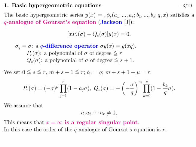
The basic hypergeometric series y(x) = rϕs(a1, ..., ar; b1, ..., bs; q, x) satisfies aq-analogue of Goursat’s equation (Jackson [J]):

[xPr(σ)−Qs(σ)]y(x) = 0.

σq = σ: a q-difference operator σy(x) = y(xq).Pr(σ): a polynomial of σ of degree ≦ rQs(σ): a polynomial of σ of degree ≦ s+ 1.

We set 0 ≦ s ≦ r, m+ s+ 1 ≦ r; b0 = q; m+ s+ 1 + µ = r:

Pr(σ) = (−σ)µr∏

j=1

(1− ajσ), Qs(σ) = −(−σ

q

)m s∏k=0

(1− bkqσ).

We assume thata1a2 · · · ar = 0,

This means that x = ∞ is a regular singular point.In this case the order of the q-analogue of Goursat’s equation is r.

2. Differential case: Mellin transform –4/29–

shifted factorial: (a)n =Γ(a+ n)

Γ(a)Generalized hypergeometric series

y(x) = pFq

(a1, ..., apb1, ..., bq

;x

)=

∞∑n=0

(a1)n · · · (ap)n(b1)n · · · (bq)nn!

xn

satisfies Goursat’s equation (ϑ = xd

dx):

[ϑ(ϑ+ b1 − 1) · · · (ϑ+ bq − 1)− x(ϑ+ a1) · · · (ϑ+ ap)] y = 0.

The Mellin Transform

g(s) := M(f ; s) =

∫ ∞

0

xs−1y(x) dx.

satisfies the following first order difference equation:

g(s+ 1) = −s(b1 − s− 1) · · · (bq − s− 1)

(a1 − s− 1) · · · (ap − s− 1)g(s)

g(s) can be represented by a product quotient of the Gamma functions.

Remark. –5/29–

g1(s+ 1) = a1(s)g1(s), g2(s+ 1) = a2(s)g2(s)⇒ g1(s+ 1)g2(s+ 1) = a1(s)a2(s)g1(s)g2(s).

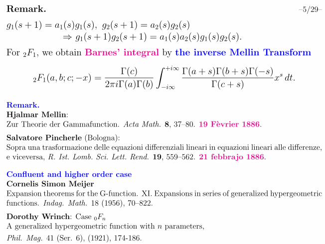
For 2F1, we obtain Barnes’ integral by the inverse Mellin Transform

2F1(a, b; c;−x) =Γ(c)

2πiΓ(a)Γ(b)

∫ +i∞

−i∞

Γ(a+ s)Γ(b+ s)Γ(−s)

Γ(c+ s)xs dt.

Remark.Hjalmar Mellin:Zur Theorie der Gammafunction. Acta Math. 8, 37–80. 19 Fevrier 1886.

Salvatore Pincherle (Bologna):Sopra una trasformazione delle equazioni differenziali lineari in equazioni lineari alle differenze,e viceversa, R. Ist. Lomb. Sci. Lett. Rend. 19, 559–562. 21 febbrajo 1886.

Confluent and higher order caseCornelis Simon MeijerExpansion theorems for the G-function. XI. Expansions in series of generalized hypergeometricfunctions. Indag. Math. 18 (1956), 70–822.

Dorothy Wrinch: Case 0Fn

A generalized hypergeometric function with n parameters,

Phil. Mag. 41 (Ser. 6), (1921), 174-186.

Letter of G. G. Stokes to his wife on March 19 1857 –6/29–

Memoir and scientific correspondence of the late Sir George Gabriel Stokes,Vol.1, p.62

3. The Newton-Puiseux diagram and irregular singularity –7/29–

The Newton-Puiseux diagram of a linear q-difference equation

an(x)u(xqn) + an−1(x)u(xq

n−1) + · · ·+ a0(x)u(x) = 0

at the origin is a lower convex hull of

{(j, ord aj(x)) ∈ R2 | 0 ≤ j ≤ n}

segment: a line jointed with (j, ord aj(x)) and (k, ord ak(x)) (j < k)slope of a segment:

µ =ord ak(x)− ord aj(x)

k − j

length of a segment: m = k − j

3.1 Irregular singular points –8/29–

General Theorem (Adams [A])1) If partial characteristic exponents λj are non-resonant for any segmentwith the slope µ and the length m, the q-difference equation has m formalsolutions

uj(x) = θ(x)µθq(x)

θq(λjx)

∑k≥0

ukxk,

for each segment

2) When the slope of a segment is not integer µ = r/s (s > 0), formal solutionsare given by formal power series of x1/s.

3) When a segment contains (0, ord a0(x)), the power series are convergent.

Problem:1) Determine the connection matrix P (x) for q-Goursat’s equation.2) For a divergent power series, find a good resummation method

4.1. Degeneration of q-hypergeometric equations –9/29–

Classification of q-hypergeometric equations of the second order

[(a2 + b2x)σ2q + (a1 + b1x)σq + (a0 + b0x)]u(x) = 0

a0 a1 a2

b0 b1 b2 s s ss s s(1)

s s ss s cccc

(2)

s s sc c s!!

!!!

(3-1)

s s sc s c###ccc

(3-2)

c s ss s ccccccc

(3-3)

s c sc s c###ccc

(4-1)

c s ss c cccc

aaaaa

(4-2)

red line: divergent

Degeneration scheme

2ϕ1(a, b; c; z) q-confluent

1ϕ1(a; 0; z)

J(3)ν

J(1)ν ∼ J

(2)ν

q-Airy

Ramanujan- �

��3

-

-

QQQs ��*

PPPq

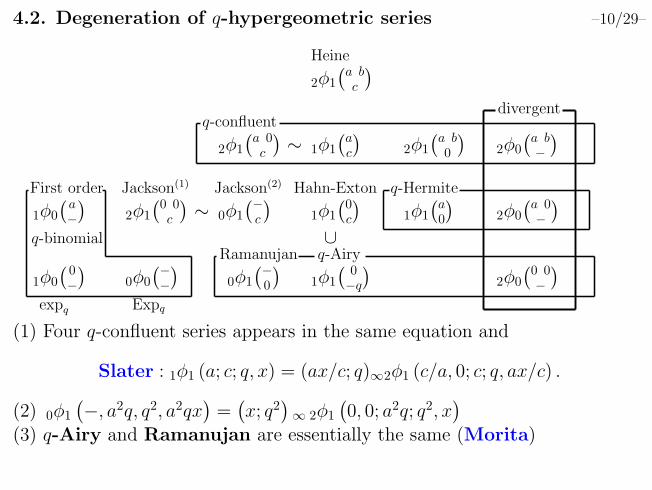
4.2. Degeneration of q-hypergeometric series –10/29–

Heine

2ϕ1

(a bc

)2ϕ1

(a 0c

)1ϕ1

(ac

)2ϕ1

(a b0

)2ϕ0

(a b−)

∼

1ϕ0

(a−)

q-binomial

2ϕ1

(0 0c

)0ϕ1

(−c

)1ϕ1

(0c

)1ϕ1

(a0

)2ϕ0

(a 0−)

∼∪

1ϕ0

(0−)

expq

0ϕ0

(−−)

Expq

1ϕ1

(0−q

)0ϕ1

(−0

)2ϕ0

(0 0−)

q-confluent

q-Hermite

q-AiryRamanujan

First order Jackson(1) Jackson(2) Hahn-Exton

divergent

(1) Four q-confluent series appears in the same equation and

Slater : 1ϕ1 (a; c; q, x) = (ax/c; q)∞2ϕ1 (c/a, 0; c; q, ax/c) .

(2) 0ϕ1

(−, a2q, q2, a2qx

)=(x; q2

)∞ 2ϕ1

(0, 0; a2q; q2, x

)(3) q-Airy and Ramanujan are essentially the same (Morita)

5.1. Connection Formula: regular singular case –11/29–

Heine 2ϕ1(a, b; c;x):

(c− abqx)u(xq2)− [c+ q − (a+ b)qx]u(qx) + q(1− x)u(x) = 0.

Local solution at x = 0 :

u1 = 2ϕ1 (a, b; c;x) , u2 =θ(−x)

θ(−qx/c)2ϕ1

(qa/c, qb/c; q2/c;x

).

Local solution at x = ∞ :

v1 =θ(−ax)

θ(−x)2ϕ1 (a, aq/c; aq/b; cq/abx) , v2 = (a ↔ b).

Theorem (Thomae, Watson) Connection formula of 2ϕ1

u1 =(b, c/a; q)∞(c, b/a; q)∞

v1 +(a, c/b; q)∞(c, a/b; q)∞

v2,

u2 =(qb/c, q/a; q)∞(q2/c, b/a; q)∞

θ(−qax/c)θ(−x)

θ(−qx/c)θ(−ax)v1 +

(qa/c, q/b; q)∞(q2/c, a/b; q)∞

θ(−qbx/c)θ(−x)

θ(−qx/c)θ(−bx)v2.

5.2. Integral representation of hypergeometric series –12/29–

Barnes’ integral

2F1(a, b; c;−x) =Γ(c)

2πiΓ(a)Γ(b)

∫ +i∞

−i∞

Γ(a+ s)Γ(b+ s)Γ(−s)

Γ(c+ s)xs dt.

We obtain the connection formula directly from Barnes’ integral.

5.3. q-analogue of the Barnes-Meijer integral –13/29–

Take a contour integral (Slater, Askey-Roy, Gasper-Rahman)∫|z|=ε

(a1z, a2z, ..., aAz, b1/z, ..., bB/z; q)∞(c1z, c2z, ..., cCz, d1/z, ..., dD/z; q)∞

dz.

The contour round z = 0 counterclockwisely and

z = 1/cjqk (j = 1, 2, ..., C; k ∈ Z≧0), z = dlq

m (l = 1, 2, ..., D;m ∈ Z≧0)

1/cjqk are outside、dlq

m are inside:

æ

ææ

æ

æ

æ

æ

æ

æ

æ

æ

æ

æ

æ

æ

-2 -1 1 2

-2

-1

1

2

5.4. Proof of connection formula of 2ϕ1 –14/29–

We set A = C = 2, B = D = 1 and

a1 = c, a2 = q/z; b1 = z; c1 = a, c2 = b; d1 = 1

We get

P (t) =(ct, qt/z, z/t; q)∞(at, bt, 1/t; q)∞

and the contour integral around t = 0:∫K

P (t) dt =(c, q/z, z; q)∞(q, a, b; q)∞

×∞∑n=0

(a, b, q/z; q)n(q, c, b/a; q)n

zn

=(c, q/z, z; q)∞(q, a, b; q)∞

2ϕ1(a, b; c; q, z) = (1)

The contour integral around t = ∞:∫K

P (t) dt =(az, c/a, q/az; q)∞

(q, a, b/a; q)∞×

∞∑n=0

(a, qa/c, az; q)n(q, az, qa/b; q)n

( cq

abz

)n+ (a ↔ b) = (2)

Since (1)=(2), we obtain the Thomae’s connection formula.

6. Connection problems and q-Stokes phenomenon –15/29–

[I] Apply q-Borel transform [Zhang, Ramis, Sauloy]

1) The q-Borel transformation B±q : C[[t]] → C[[τ ]] is defined by

B±q

[ ∞∑n=0

antn

]:=

∞∑n=0

anq±n(n−1)/2τn.

q-Borel Transform of equationsLemma As a linear operator on C[[t]], we have

B±q (t

mσnq f) = q±m(m−1)/2τmσn±m

q B±q (f).

[II] When a solution is a convergent power series:1) ϕ(τ) = B−

q (f)(τ) satisfies a first order equation and has a form

φ(τ) =(a1τ, · · · , akτ ; q)∞(b1τ, · · · , bmτ ; q)∞

, (k < m)

2) The residue calculus of L−q (ϕ)(t) gives a connectin formlua

L−q (φ)(t) =

1

2πi

∫|τ |=ε

φ(τ)θq(t/τ)dτ

τ.

6.1 q-Stokes phenomenon: irregular singular case –16/29–

[III] When a solution is a divergent power series:

1) The q-Borel transform B+q (f) satisfies an equation of the same order

2) B+q (f) may be convergent and reduces to the case [II]

3) Solve the connection problem for B+q (f) on the Borel plane.

4) Apply the q-Laplace transform L[λ]q;1 (λ ∈ C×):

The q-Laplace transform L[λ]q;1 is given by the Jackson integral

L[λ]q;1(φ)(x) :=

1

1− q

∫ λ∞

0

φ(τ)

θq(τ/x)

dqτ

τ=

∞∑n∈Z

φ(qnλ)

θq(qnλ/x).

⋆ When f(t) ∈ C[[t]] is convergent, L[λ]q;1 is an inverse of B+

q

⋆ The RHS has poles at x ∈ −λqZ. By the q-Borel-Laplace resummation,

f(x, λ) := L[λ]q;1 ◦ B+

q (f)

is a holomorphic function {0 < |x| < ε} \ −λqZ and asymptotic to f .

The q-Stokes region is an open dense set in C×, not an angledomain. For q-divergence series, the q-Stokes region depends on acontinuous parameter λ.

6.2 Strategy –17/29–

We change q-difference equation by the following two transformations:

Lemma 1. (1) The q-Borel transformation B±q satisfies

B±q (t

mσnq f) = q±m(m−1)/2τmσn±m

q B±q (f).

(2) The theta function shifts the power of x:

xmσnq

[θ(cx)±1f(x)

]= c∓nq∓n(n−1)/2xm∓nθ(cx)±1σn

q f(x).

c s s ss s s sQQQ

=⇒(2) s s s sc s s s

���������

������ =⇒

(1) ssss

ssscQ

QQ

Remark.In general, q-difference equations have less transform than differential equa-tions. We can change q-difference equations to ‘first order’ equations by thetwo transformations in the above lemma.

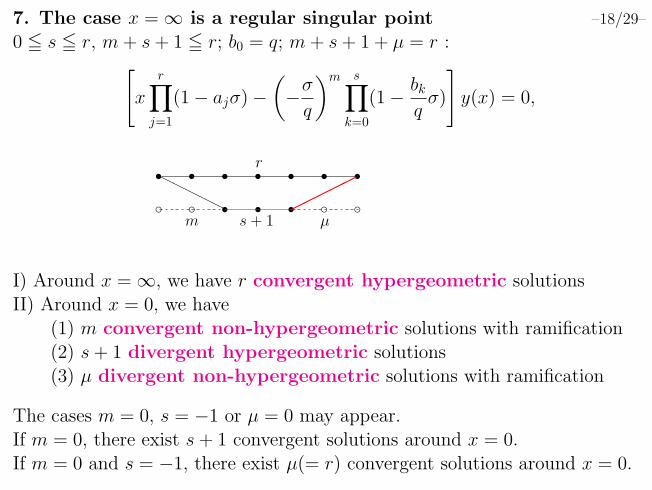
7. The case x = ∞ is a regular singular point –18/29–

0 ≦ s ≦ r, m+ s+ 1 ≦ r; b0 = q; m+ s+ 1 + µ = r :[x

r∏j=1

(1− ajσ)−(−σ

q

)m s∏k=0

(1− bkqσ)

]y(x) = 0,

r

m s+ 1 µc c s s s c cs s s s s s sHHHHH �����

I) Around x = ∞, we have r convergent hypergeometric solutionsII) Around x = 0, we have

(1) m convergent non-hypergeometric solutions with ramification(2) s+ 1 divergent hypergeometric solutions(3) µ divergent non-hypergeometric solutions with ramification

The cases m = 0, s = −1 or µ = 0 may appear.If m = 0, there exist s+ 1 convergent solutions around x = 0.If m = 0 and s = −1, there exist µ(= r) convergent solutions around x = 0.

7.1 Local solutions –19/29–Local solutions around the infinity (j = 1, ..., r)

yj,∞(x) =θ(−ajx)

θ(−x)m+sϕr−1

(qaj/b0, qaj/b1, ...., qaj/bs,0

qaj/aj+1, qaj/aj+2, ...., qaj/aj−1,; q,

qµar+1j b0b1 · · · bs

a1a2 · · · arx

)

Formal divergent solutions at the origin (k = 0, ..., s)

yk,0(x) =θ(−x)

θ(−qx/bk)rϕs−1

(qa1/bk, qa2/bk, ..., qar/bk

qbk+1/bk, qbk+2/bk, ..., qbk−1/bk; q, x

)Ramified convergent solutions at the origin (k = 1, ...,m)

x = zm and q = pm. ωm = 1.

uk,0(z) =1

θp(−p(m+1)/2ωkz)vk(z), vk(z) =

∞∑n=0

v(k)n zn.

Ramified divergent solutions at the origin (k = 1, ..., µ)µ = r − s− 1, x = zµ and q = pµ. ωµ = 1. cµ = a1a2 · · · ar/b0b1 · · · bs.

wk,0(z) = θp(−c p(1−µ)/2ωkz)hk(z), hk(z) =∞∑n=0

h(k)n zn.

7.2 Watson’s formula: Covergent to Convergent –20/29–

Assume that m = 0 [W].

Theorem 2. We assume that 0 ≦ s < r. Then

rϕr−1

(a1, ..., ar

b1, ..., bs, 0, ..., 0; q, z

)=

(a2, ..., ar+1, bs/a1, ...bs/a1; q)∞(b1, ..., bs, a2/a1, ..., ar/a1; q)∞

×θ(−a1z)

θ(−z)s+1ϕr−1

(qa1/b0, qa1/b1, ..., qa1/bs

qa1/a2, ..., qa1/ar; q, (a1q)

r−s−1b0b1 · · · bsa1 · · · arz

)+idem(a1; a2, ..., ar).

LHS is convergent when |z| < 1 and RHS is convergent when s < r − 1 ors = r − 1 and |qb1 · · · bs/a1 · · · arz| < 1.

Proof is easy from a contour integral.We consider a contour integral

I =1

2πi

∫K

(b1t, ..., bst, qt/z, z/t; q)∞(a1t, ..., art, 1/t; q)∞

dt

t.

Here the contour K rounds once the origin counterclockwisely.

7.2 Ramified case –21/29–

m > 0, pm = q. We assume that s+m ≧ r.

I =

∫|τ |=ε

∏sj=1(bjτ ; q)∞∏rk=1(akτ ; q)∞

θp(x/τ)dτ

τ

=(b1/a1, ..., bs/a1; q)∞(q, a2/a1, ...ar/a1; q)∞

θp(a1x)

× s+mϕr−1

(qa1/b1, ..., qa1/bs,0m

qa1/a2, ..., qa1/ar; q,

(−1)rqr−s+(1−m)/2b1 · · · bsam−r+11 a2 · · · arx

)+ idem(a1; a2, ..., ar).

[Useful relation]

Resτ=1/aqn1

(aτ ; q)∞

dτ

τ= −(−1)nqn(n+1)/2

(q; q)∞(q; q)n,

θp(x/τ)|τ→1/aqn = (ax)−mnp−nm(nm−1)/2θp(ax),

(bτ ; q)∞|τ→1/aqn = (−b/a)nq−n(n+1)/2(b/a; q)∞(aq/b; q)n.

7.3 q-Borel-Laplace transformation: –22/29–

I) Unramified caseAny divergent hypergeometric series is unramified.The qm-Borel Laplace transform is convergent hypergeometric series.

m s+ 1 µ

=⇒B+qmc c s s s c c

s s s s s s ss s s c c c cs s s s s s sHHHHH

�����

�����

II) Ramified case

Lemma 3. We take a positive integer m. We consider

φ(ξ) =θq(aξ)

θq(bξ)

∑n≥0

cnξ−n.

Then we obtain

L[λ]qm;1φ(x) =

θq(aλ)θqm(qmamx/bmλ)

θq(bλ)θqm(qmx/λ)

∑n≥0

cn(qm)−

n(n−1)2

(bm

amqmx

)n

.

8. Main Theorem –23/29–

The basic hypergeometric series y(x) = rϕs(a1, ..., ar; b1, ..., bs; q, x) satisfies aq-analogue of Goursat’s equation :[

x

r∏j=1

(1− ajσ)−(−σ

q

)m s∏k=0

(1− bkqσ)

]y(x) = 0,

r

m s+ 1 µc c s s s c cs s s s s s sHHHHH �����

Theorem 1. If r = 2, we have seven different hypergeometric-typeequations. All of connection formula are determined. The q-Stokes regions areopen dense domains C× \ λqZ.Thomae [Th], Watson [W], Slater [S1], Zhang [Z02, Z03], Morita [M1], O.

Theorem 2. If r = 3 and aj = 0, we have ten different hypergeometric-type equations. All of connection formula are determined. The q-Stokesregions are open dense domains C× \ λqZ. (Except Q = 1)By Thomae [Th2], Watson [W], Morita[M2], Zhang, O. Adachi [Ad]

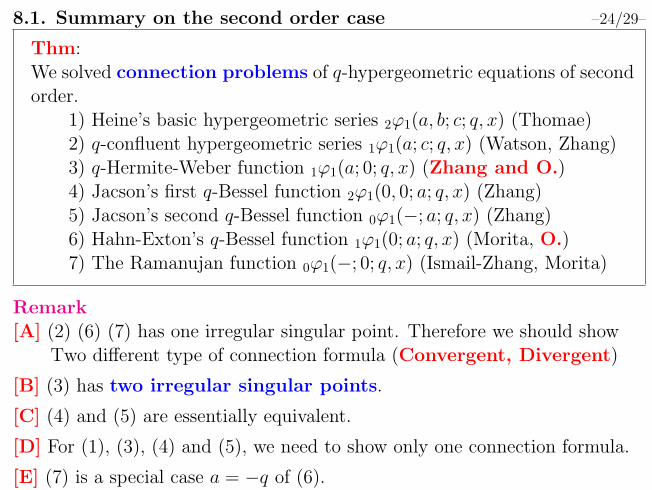
8.1. Summary on the second order case –24/29–

Thm:We solved connection problems of q-hypergeometric equations of secondorder.

1) Heine’s basic hypergeometric series 2φ1(a, b; c; q, x) (Thomae)2) q-confluent hypergeometric series 1φ1(a; c; q, x) (Watson, Zhang)3) q-Hermite-Weber function 1φ1(a; 0; q, x) (Zhang and O.)4) Jacson’s first q-Bessel function 2φ1(0, 0; a; q, x) (Zhang)5) Jacson’s second q-Bessel function 0φ1(−; a; q, x) (Zhang)6) Hahn-Exton’s q-Bessel function 1φ1(0; a; q, x) (Morita, O.)7) The Ramanujan function 0φ1(−; 0; q, x) (Ismail-Zhang, Morita)

Remark[A] (2) (6) (7) has one irregular singular point. Therefore we should show

Two different type of connection formula (Convergent, Divergent)

[B] (3) has two irregular singular points.

[C] (4) and (5) are essentially equivalent.

[D] For (1), (3), (4) and (5), we need to show only one connection formula.

[E] (7) is a special case a = −q of (6).

9.1 Example: q-Stokes phenomenon of Hahn-Exton’s q-Bessel –25/29–Modified Hahn-Exton’s q-Bessel function:

qtv(tq) + [1− (a+ q)t]v(t) + atv (t/q) = 0. c s cs s s@@@ �

��

Local solutions around t = ∞

v(∞)1 (t) = 1φ1(0; a; q, 1/t), v

(∞)2 (t) =

θ(qt/a)

θ(t)1φ1(0; q

2/a; q, q/at).

Local (meromorphic) solutions around t = 0

(C) v(0)2 (t) =

1

θ(−aqt)

∞∑m=0

cmtm, (D) v

(0)1 (t) = θ(−qt)

∞∑m=0

bmtm.

We need to take q1/2-Borel transformation (Dreyfus, Eloy [DE] [El])

Hahn-Exton

c s cs s sccc#

## -

mutiply θ(x)

c s sc s csTTTTT

ccccc

-

Consider as q1/2-difference

c c s c sc c s c csccccc

aaaaaaaaaa

T q1/2-Borel transform

c c s c sc c c s cc c s c cccccc

-

The last equation is reduced to the second Jackson q-Bessel [Z03].

By the q1/2-Laplace transform L[λ]

q1/2;1, we get the Hahn-Exton [O3].

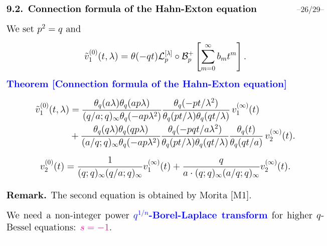
9.2. Connection formula of the Hahn-Exton equation –26/29–

We set p2 = q and

v(0)1 (t, λ) = θ(−qt)L[λ]

p ◦ B+p

[ ∞∑m=0

bmtm

].

Theorem [Connection formula of the Hahn-Exton equation]

v(0)1 (t, λ) =

θq(aλ)θq(apλ)

(q/a; q)∞θq(−apλ2)

θq(−pt/λ2)

θq(pt/λ)θq(qt/λ)v(∞)1 (t)

+θq(qλ)θq(qpλ)

(a/q; q)∞θq(−apλ2)

θq(−pqt/aλ2)

θq(pt/λ)θq(qt/λ)

θq(t)

θq(qt/a)v(∞)2 (t).

v(0)2 (t) =

1

(q; q)∞(q/a; q)∞v(∞)1 (t) +

q

a · (q; q)∞(a/q; q)∞v(∞)2 (t).

Remark. The second equation is obtained by Morita [M1].

We need a non-integer power q1/n-Borel-Laplace transform for higher q-Bessel equations: s = −1.

9.3 Example: 3ϕ2 (a1, a2, a3; b1, 0; q, x) –27/29–[x

3∏j=1

(1− ajσ)− (1− σ)(1− b1qσ)

]y(x) = 0.

Local solutions around the origin:

y1,0(x) = 3ϕ2

(a1, a2, a3b1, 0

; q, x

),

y2,0(x) =θ(−x)

θ(−qx/b1)3ϕ2

(a1q/b1, a2q/b1, a3q/b1

q2/b1, 0; q, x

),

y3,0(x) = θ(−a1a2a3x/b1q)w(x), w(x) =∞∑n=0

wnxn.

Local solutions around the infinity:

y1,∞(x) =θ(−a1x)

θ(−x)2ϕ2

(a1, a1q/b1

a1q/a2, a1q/a3; q,

q2b1a2a3x

)y2,∞(x), y3,∞(x) are cyclic

We set v(ξ) = B+q (w). –28/29–

(1 + s3ξ/a1b1q)(1 + s3ξ/a2b1q)(1 + s3ξ/a3b1q)v(ξq)

=(1 + s3ξ/b21q)(1 + s3ξ/b1q

2)v(ξ).

Therefore

v(ξ) =(−s3ξ/qa1b1,−s3ξ/qa2b1,−s3ξ/qa2b1)∞

(−s3ξ/q2b1,−s3ξ/qb21)∞.

We set

y3(x, λ) = θ(−s3x/b1q)L[λ]q;1 ◦ B+

q [w](x) = θ(−s3x/b1q)L[λ]q;1[v](x).

Theorem

y3(x, λ) =(q, b1/a1, q/a1; q)∞(a2/a1, a3/a1; q)∞

θ(qa2b1/s3λ, qa3b1/s3λ)

θ(qb21/s3λ, q2b1/s3λ)

× θ(−s3x/qb1, qa1b1x/s3λ)

θ(−a1x, x/λ)y1,∞(x) + idem(a1; a2, a3).

Connection formulae of y1(x), y2(x) are obtained by Watson’s formula.

Future Problem –29/29–

We find connection formulae for basic hypergeometric equations.Our methods can be applied to other equations.

[Problem]1) Connection formula in the case both x = 0 and x = ∞ are irregular.

2) I forget Q = 1 case...

3) Find a connection formula of other rigid q-difference equations

4) Find a connection formula of confluent q-Appell equations

5) Apply to q-Heun or q-Painleve equations (Vinet)

6) How about confluent elliptic hypergeometric equation? (Noumi)

7) Application to many fields in mathematical sciences (Sasamoto, ...)

8) Relation to q-difference Galois theory (Duval-Mitschi, Roques)

9) What is q-WKB method, q-resurgent analysis or q-Ecalle? (Joshi)

Lucy Joan Slater

These photos were provided from the archives of the Dalton GenealogicalSociety.Check out “daltonhistory.org”!

“A Woman in a Man’s World” ed. John Dalton, 2013.

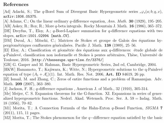
References

[Ad] Adachi, S.; The q-Borel Sum of Divergent Basic Hypergeometric series rφs(a; b; q, x),arXiv:1806.05375.[A] Adams, C.; On the linear ordinary q-difference equation, Ann. Math. 30 (1929), 195–205.[AR] Askey, R.; Roy, R.; More q-beta integrals. Rocky Mountain J. Math. 16 (1986), 365–372.[DE] Dreyfus, T., Eloy, A.; q-Borel-Laplace summation for q-difference equations with twoslopes, arXiv:1501.02994 [math.CV].[DM] Duval, A.; Mitschi, C.; Matrices de Stokes et groupe de Galois des equations hy-pergeometriques confluentes generalisees. Pacific J. Math. 138 (1989), 25–56.[El] Eloy, A.; Classification et geometrie des equations aux q-differences: etude globale deq-Painleve, classification non isoformelle et Stokes a pentes arbitraires, These, Universite deToulouse, 2016. [http://thesesups.ups-tlse.fr/3376/][GR] G. Gasper and M. Rahman, Basic Hypergeometric Series, 2nd ed, Cambridge, 2004.[HKW] Hamamoto, T.; Kajiwara, K.; Witte, N.; Hypergeometric solutions to the q-Painleveequation of type (A1 + A′

1)(1). Int. Math. Res. Not. 2006, Art. ID 84619, 26 pp.[IZ] Ismail, M. and Zhang, C.; Zeros of entire functions and a problem of Ramanujan. Adv.Math. 209 (2007), 363–380.[J] Jackson, F. H.; q-difference equations , American J. of Math., 32 (1910), 305-314.[Me] Meijer, C. S. Expansion theorems for the G-function. XI. Expansions in series of gener-alized hypergeometric functions. Nederl. Akad. Wetensch. Proc. Ser. A. 59 = Indag. Math.18 (1956), 70–82.[M1] Morita, T.; A Connection Formula of the Hahn-Exton q-Bessel Function, SIGMA 7(2011), 115, 11 pages.[M2] Morita, T.; The Stokes phenomenon for the q−difference equation satisfied by the basic

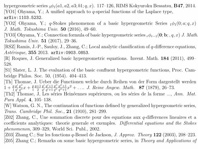
hypergeometric series 3ϕ1(a1, a2, a3; b1; q, x). 117–126, RIMS Kokyuroku Bessatsu, B47, 2014.[YO1] Ohyama, Y.; A unified approach to q-special functions of the Laplace type,arXiv:1103.5232.[YO2] Ohyama, Y.; q-Stokes phenomenon of a basic hypergeometric Series 1ϕ1(0; a; q, x)J. Math. Tokushima Univ. 50 (2016), 49–60.[YO3] Ohyama, Y.; Connection formula of basic hypergeometric series rϕr−1(0;b; , q, x) J. Math.Tokushima Univ. 51 (2017), 29–36.[RSZ] Ramis, J.-P., Sauloy, J., Zhang, C.; Local analytic classification of q-difference equations,Asterisque, 355 2013. arXiv:0903.0853.[R] Roques, J. Generalized basic hypergeometric equations. Invent. Math. 184 (2011), 499–528.[S1] Slater, L. J. The evaluation of the basic confluent hypergeometric functions, Proc. Cam-bridge Philos. Soc. 50, (1954). 404–413.[Th] Thomae, J. Ueber die Functionen welche durch Reihen von der Form dargestellt werden1 + p

1p′

q′p′′

q′′x+ p

1p+12

p′

q′p′+1q′+1

p′′

q′′p′′+1q′′+1

x2 + . . .. J. Reine Angew. Math. 87 (1879), 26–73.

[Th2] Thomae, J, Les series Heineennes superieures, ou les series de la forme ..., Ann. Mat.Pura Appl. 4, 105–138.[W] Watson, G. N., The continuation of functions defined by generalized hypergeometric series,Trans. Cambridge Phil. Soc., 21 (1910), 281–299.[Z02] Zhang, C., Une sommation discrete pour des equations aux q-differences lineaires et acoefficients analytiques: theorie generale et exemples. Differential equations and the Stokesphenomenon, 309–329, World Sci. Publ., 2002.[Z03] Zhang C.; Sur les fonctions q-Bessel de Jackson, J. Approx. Theory 122 (2003), 208–223.[Z05] Zhang C.; Remarks on some basic hypergeometric series, in Theory and Applications of

Special Functions, Dev. Math., Vol. 13, Springer, New York, 2005, 479–491.