z) 0(m2/3). - california institute of...

SIAM J. ScI. COMPUT.Vol. 17, No. 2, pp. 454-478, March 1996

() 1996 Society for Industrial and Applied Mathematics010

ALTERNATING-DIRECTION LINE-RELAXATION METHODS ONMULTICOMPUTERS*

J)RN HOFHAUS AND ERIC E VAN DE VELDE$

Abstract. We study the multicomputer performance of a three-dimensional Navier-Stokes solver based onalternating-direction line-relaxation methods. We compare several multicomputer implementations, each of whichcombines a particular line-relaxation method and a particular distributed block-tridiagonal solver. In our experiments,the problem size was determined by resolution requirements of the application. As a result, the granularity of thecomputations of our study is finer than is customary in the performance analysis of concurrent block-tridiagonalsolvers. Our best results were obtained with a modified half-Gauss-Seidel line-relaxation method implemented bymeans of a new iterative block-tridiagonal solver that is developed here. Most computations were performed on theIntel Touchstone Delta, but we also used the Intel Paragon XP]S, the Parsytec SC-256, and the Fujitsu S-600 forcomparison.

Key words. Navier-Stokes equations, concurrency, parallelism, block-tridiagonal systems, tridiagonal systems,ADI, alternating directions

AMS subject classifications. 65M20, 65N40, 65Y05, 76C05, 76M20

1. Introduction. When using alternating-direction line-relaxation methods for systemsof partial-differential equations discretized on a rectangular grid, one must solve many block-tridiagonal systems of linear equations in every relaxation step. This type of computationsurfaces in many applications. In our work, we faced it when parallelizing a highly vectorizedsolver for the three-dimensional, unsteady, and incompressible Navier-Stokes equations [4]for use on multicomputers. In this paper, we shall discuss and analyze five line-relaxationmethods and six distributed block-tridiagonal solvers used during the course of this project.We have measured the performance of several combinations of relaxation methods and block-tridiagonal solvers on three multicomputers (the Intel Touchstone Delta [5], the Intel ParagonXP/S [6], and the Parsytec SC-256 13]) and on one conventional vector processor (the Fujitsus-600).

Three-dimensional computations are more complex thantwo-dimensional ones because ofadditional coordinates for the geometry and the vector fields. Three-dimensional computationsare also algorithmically different, because every line-relaxation step requires the solution ofa larger number of smaller-sized linear systems than a comparable two-dimensional line-relaxation step. To see this, consider a two- and a three-dimensional problem of the samesize, i.e., with the same number of unknowns. The two-dimensional problem on an M Mgrid requires the solution of O(M) block-tridiagonal systems of size O (M), while the three-dimensional problem on an N N N grid with N M2 requires the solution of O(Nz)O(M4/3) systems of size O(N) 0(M2/3).

On multicomputers, the reduced system size has a serious impact. There exist manyconcurrent algorithms to solve block-tridiagonal systems; see, e.g., [2], [10], [12], [14]-[16].However, these methods have been studied mainly for very coarse-grain computations, i.e., forcomputations in which the ratio ofthe system size over the number ofnodes is high. Bondeli [2]studied computations with less than 25 nodes and system sizes exceeding 16, 800. Krechel,

*Received by the editors August 16, 1993; accepted for publication (in revised form) October 24, 1994. Thismaterial is based upon work supported by the NSF under Cooperative Agreement No. CCR-9120008. Access to theIntel Touchstone Delta was provided by the Concurrent SuperComputing Consortium.

tAerodynamisches Institut der RWTH Aachen, Wiillnerstr. zw. 5 u. 7, 52062 Aachen, Germany (jorn@a +/- a. rwth- aachen. de). Caltech visit sponsored by the German Research Association (DFG) within the project:Strrmungssimulation mit Hochleistungsrechnern.

tApplied Mathematics 217-50, California Institute of Technology, Pasadena, CA 91125 (evdv@ama. caltech, edu).

454

ADI METHODS ON MULTICOMPUTERS 455

Plum, and Stiiben 14] improved the efficiency of a modified cyclic-reduction algorithm onthe 16-node iPSC/2-VX. Their computations of moderate-to-coarse granularity solved 256tridiagonal systems of size 128 and the highest-achieved efficiency was about 50%. Forthe reasons mentioned above, the granularity of the block-tridiagonal solver in our three-dimensional application is much smaller when running the code for a grid of fixed size onall 512 computing nodes of the Delta. Constructing an efficient concurrent program for thisproblem is a challenge.

An outline of the paper follows. In 2, a brief description of the implemented relaxationmethods is given. In 3, we shall study algorithm and concurrency issues of several basicconcurrent alternating-direction relaxation methods. Each method is based on a different dis-tributed solver for block-tridiagonal systems. First, the sequential block-tridiagonal solver isdistributed and pipelined to obtain a concurrent line-relaxation method: Subsequently, we useconcurrent tridiagonal solvers based on recursive doubling, cyclic reduction, partitioning, anddivide and conquer, respectively. Finally, a new iterative tridiagonal solver is developed. In 4,we analyze the performance on the Delta of the proposed methods applied to a Navier-Stokessolver. The Navier-Stokes equations and their discretization for an interesting application aregiven in 4.1. We give this description for the sole purpose of defining precisely how the per-formance data were obtained. The fluid-dynamical results of our computations are discussedin another paper 1]. In 5, computations on the Paragon, the Parsytec, and the Fujitsu arecompared with those on the Delta.

2. Relaxation methods. The discretization of partial-differential equations often leadsto a large sparse system of equations

(1) A-- f.Classical relaxation methods to solve (1) are obtained by splitting the coefficient matrix A into

A=G+H

with G an easily inverted matrix. This defines the iteration

(2) f- H-,which converges to the exact solution t* if the spectral radius of G-H is less than one; e.g.,see 11].

In the description that follows, it is convenient to think of the three-dimensional Poissonproblem discretized to second-order accuracy on a three-dimensional rectangular grid of sizeM N K. Then, interior grid points are identified by means of a triple (m, n, k) with1 _< m < M, 1 < n < N, and 1 < k < K. One unknown and one equation is associated witheach interior grid point.

One elementary line-relaxation step updates all unknowns ofone grid line simultaneously.For example, an x-line is a set of grid points (m, n, k) where 1 _< m < M and n and k are fixed.An x-line is, therefore, identified by means of a couple (n, k). An elementary x-line-relaxationstep reduces to the tridiagonal system

(3) am Um-1 + bm Um + Cm Um+l dm, m 1 M

for each x-line. One x-line-relaxation step updates all x-lines ofthe grid once, i.e., it performsan elementary x-line-relaxation step for all (n, k) with < n < N and 1 < k < K. Forthree-dimensional problems, an alternating-direction line-relaxation step consists of an x-line-relaxation step, a y-line-relaxation step, and a z-line-relaxation step. We restrict ourdiscussion to the x-line-relaxation step. In matrix-vector notation, the system (3) has the form

(4) T t =,

456 JORN HOFHAUS AND ERIC E VAN DE VELDE

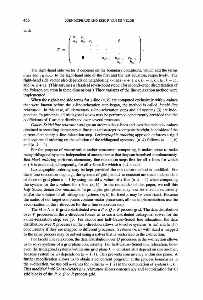
with

bl Cla2 b2 C2 0

0 aM-1 bM-1 CM-1aM bM

The right-hand side vector d depends on the boundary conditions, which add the terms

aluo and CMUM+I to the fight-hand side of the first and the last equation, respectively. Theright-hand side vector also depends on neighboring x-lines (n + 1, k), (n 1, k), (n, k 1),and (n, k + 1). (This assumes a classical seven-point stencil for second-order discretization ofthe Poisson equation in three dimensions.) Three variants of the line-relaxation method wereimplemented.

When the right-hand side terms for x-line (n, k) are computed exclusively with u-valuesthat were known before the x-line-relaxation step began, the method is called Jacobi linerelaxation. In this case, all elementary x-line-relaxation steps and all systems (3) are inde-pendent. In principle, all tridiagonal solves may be performed concurrently provided that thecoefficients of T are not distributed over several processes.

Gauss-Seidel line relaxation assigns an order to the x-lines and uses the updated u-valuesobtained in preceding elementary x-line-relaxation steps to compute the right-hand sides ofthecurrent elementary x-line-relaxation step. Lexicographic ordering approach enforces a rigidand sequential ordering on the solution of the tridiagonal systems: (n, k) follows (n 1, k)and (n, k 1).

For the purpose of vectorization and/or concurrent computing, it makes sense to makemany tridiagonal systems independent ofone another so that they canbe solved simultaneously.Red-black ordering performs elementary line-relaxation steps first for all x-lines for whichn + k is even and, subsequently, for all x-lines for which n + k is odd.

Lexicographic ordering may be kept provided the relaxation method is modified. Forthe x-line-relaxation step, e.g., the systems of grid plane k constant are made independentof those of grid plane k 1 by using the old u-values of x-line (n, k 1) when computingthe system for the u-values for x-line (n, k). In the remainder of this paper, we call this

half-Gauss-Seidel line relaxation. In principle, grid planes may now be solved concurrentlyand/or the solution of all tridiagonal systems (n, k) for fixed n may be vectorized. Becausethe nodes of our target computers contain vector processors, all our implementations use thevectorization in the z-direction for the x-line-relaxation step.

The M x N x K grid is distributed over a P x Q x R process grid. The data distributionover P processes in the x-direction forces us to use a distributed tridiagonal solver for thex-line-relaxation step; see 3. For Jacobi and half-Gauss-Seidel line relaxation, the datadistribution over R processes in the z-direction allows us to solve systems (n, k0) and (n, kl)concurrently if they are mapped to different processes. Systems (n, k) with fixed n mappedto the same process may be solved using a solver that is vectorized in the z-direction.

For Jacobi line relaxation, the data distribution over Q processes in the y-direction allowsus to solve systems of a grid plane concurrently. For half-Gauss-Seidel line relaxation, how-ever, the tridiagonal systems within one grid plane k constant still depend on one another,because system (n, k) depends on (n 1, k). This prevents concurrency within one plane. Afurther modification allows us to obtain a concurrent program: at the process boundaries inthe y-direction, we use old u-values for x-line (n 1, k) in the computation of system (n, k).This modified half-Gauss-Seidel line relaxation allows concurrency and vectorization for allgrid blocks of the P x Q x R process grid.


We shall also consider one alternative to line relaxation. Segment relaxation avoids dis-tributed tridiagonal systems by moving terms that couple the system across process boundariesto the right-hand side. For an elementary x-line-relaxation step, this leads to systems withcoefficiem matrices of the form:

( bl 1a2 b2 2

a3 b3b4 6"4a5 b5 c5

a6 b6

bM-2 CM-2aM-1 bM-1 CM-1

\ bM CM

Such systems can be solved without any communication and only require solving a tridiagonalsystem in each process. In 4.2.4, we shall see that, for our application, the price for simplicityis a decreased convergence rate and a lack of robustness.

A discussion of point-relaxation methods is omitted, because they diverge when used forour application. We focus the remainder of this paper on modified half-Gauss-Seidel line,Jacobi line, red-black line, and segment relaxation. Each has a certain convergence rate, whichis dependent on the particular application. We postpone a discussion ofconvergence rates until4, where our application is introduced.

For simplicity of exposition, the relaxation methods were described with the Poissonequation in mind. Their use in our Navier-Stokes application is more complicated, becauseevery grid point corresponds to four unknowns. In (3), the unknowns Um and the right-handside coefficients dm are vectors of dimension 4. The coefficients am, bin, and Cm are 4 x 4matrices. The coefficient matrix T of (4) is block-tridiagonal instead of tridiagonal, and itsblocks are 4 x 4 matrices.

3. Distributed block-tridiagonal solvers. In this section, we shall present several meth-ods to solve sets of block-tridiagonal systems (3) defined on an M x N x K computationalgrid that is distributed over a P x Q x R process grid. Each solver can be combined with atleast one relaxation method of 2.

In process (p, q, r) of the process grid, we have available an I x J x L subgrid ofthe computational grid. The solution of the discretized Navier-Stokes equations requiresalternating-direction line relaxations. Hence, even if the grid is distributed in one dimensiononly (say Q R 1 or P Q 1), process boundaries cross the relaxation lines inat least one direction. We consider only the x-line relaxation with systems of M equationsdistributed over P processes; the extension to y- and z-line relaxations and to nondistributedline relaxations are obvious.

We shall introduce six different distributed tridiagonal solvers. Each can be converted intoa block-tridiagonal solver that can be used to solve the systems that arise in our Navier-Stokesapplication. To convert, scalars of the tridiagonal solvers must be changed into 4 x 4 matricesor vectors of dimension 4. Divisions like

amUm b---

must be replaced by 4 x 4 systems of equations:

bmum am.

458 JIRN HOFHAUS AND ERIC F. VAN DE VELDE

For the remainder ofthis section, we treat all coefficients and unknowns as scalars and all line-relaxation systems as tridiagonal. The conversion to block-tridiagonal systems considerablycomplicates the implementation, but it does not affect the fundamental algorithmic structure.

3.1. Pipelining. The classical sequential direct solver for tridiagonal systems, sometimesreferred to as the Thomas algorithm, can be used on distributed data. Although a sequentialalgorithm, there is sufficient concurrency left, because we must solve many tridiagonal sys-tems. For all practical purposes, this solver can only be used in conjunction with the Jacobiline-relaxation method, for which all tridiagonal systems are independent of one another. Inthe y- and z-directions, the Jacobi x-line relaxation is concurrent, and the only communicationrequirement is a boundary exchange.

An elementary x-line-relaxation step uses all processes (p, q, r) with 0 < p < P andq and r fixed. We now use the J systems of the y-direction to introduce concurrency in thex-direction by a pipelining technique (this technique is also studied by Ho and Johnsson [8]).

Assuming that the coefficient matrix T is factored once, the Thomas algorithm solvestridiagonal systems by means of two elementary sequential loops. After data distributionover P processes, these loops remain sequential. In process (p, q, r), we must run throughJ identical loops..As soon as process (p, q, r) hands over the loop of system j to process(p + 1, q, r), process (p, q, r) may start evaluating the loop of system j + 1. Filling thepipeline requires P elementary x-line-relaxation steps.

This procedure is also vectorized in the z-direction: instead of evaluating the loop forone system, all L loops of the z-direction are evaluated. This also reduces communicationlatency, because messages of L systems are combined into one message. On the other hand,this merging of communication increases the time required for filling the pipeline.

3.2. Concurrent direct tridiagonal solvers. As an alternative to pipelining, it is possibleto replace the sequential tridiagonal solver by a concurrent direct tridiagonal solver. Thisavoids the cost of pipelining. However, all known concurrent direct tridiagonal solvers carry ahigh floating-point overhead. We have used four different direct solvers. From a fundamentalpoint of view, all four are equivalent. They solve a tridiagonal system by LU-decompositionwithout pivoting, and their operation counts are very similar. Performance differences are dueto technical implementation details.

To identify the different solvers, we follow the nomenclature of Frommer [7] in thispaper. Note, however, that there is no generally agreed-upon terminology in the literature.For example, the term "recursive doubling" is used for several methods [7], [15]. We shall use"recursive doubling" and "cyclic reduction" for two variants of the cyclic odd-even reductionalgorithm, first proposed by Hockney [9].

3.2.1. Recursive doubling. By eliminating unknowns and equations, one can obtaina new tridiagonal system with half the number of unknowns of the original system. Thisreduction procedure is repeated until a system is obtained that can be solved immediately.

In the recursive-doubling algorithm, one reduction is computed for each of the M equa-tions. Hence, we can determine all solution components immediately after the last reductionstep.

3.2.2. Cyclic reduction. The cyclic-reduction method also performs repeated reductionsof the system (3). However, it computes only one solvable equation for the whole system.Subsequently, the solution is computed through back-substitution.

In general, the number of equations per process, I, is greater than one. Therefore, wehave to distinguish between a local and a global reduction. In the first log2 1 steps, we reducethe system such that the unknowns are coupled exclusively with unknowns in neighboringprocesses. Each tridiagonal system now consists of only one equation per process. In the


blb2

c2c2b3 3a4 b4 C4a5 b5 c5a6 b6 6

a7 b7 c7a8 b8 c8a9 b9

FIG. 1. Matrix T after eliminating the upper and lower diagonal entries.

subsequent global reduction, we eliminate the remaining equations of the first, second, fourth,etc. neighbors.

3.2.3. Partition method. In 3.2.2, the local part of the odd-even reduction reduced thesystem to a new tridiagonal system with one equation per process. The required communica-tion and the arithmetic overhead of solving the latter system are high. This problem is avoidedin Wang’s partition method [16].

After an elimination ofthe upper and lower diagonal entries, the coefficient matrix has theshape given in Fig. 1 for a system withM 9 equations distributed over P 3 processes. Thefill that results from this operation can be stored in the original arrays am and Cm. This matrixis triangularized and, subsequently, diagonalized. For these operations, Wang transposes Tfrom a row-distributed into a column-distributed matrix. Because this transposition of thematrix requires extensive communication, we follow an alternative procedure. We solve thefollowing tridiagonal system with one equation per process:

(5) a6 b6 c6 u6 d6a9 b9 u9 d9

which is obtained by collecting the equations of the last row in each process. We solvedthe system (5) by recursive doubling, which we found to be most efficient in the case of oneequation per process.

3.2.4. Divide and conquer. In his divide-and-conquer method, Bondeli [2] obtains thesolution of (3) by solving a local tridiagonal system in each process concurrently and a globaltridiagonal system with one equation in the boundary processes and two equations in the innerprocesses.

Here, the global problem is solved by eliminating one equation in the inner processes.Again, we obtain a tridiagonal system with one equation per process which is solved withrecursive doubling.

3.3. Concurrent iterative tridiagonal solver. The direct solvers of3.2 solve the system(3) to round-off error (if the systems are well conditioned). Here, we propose a concurrentiterative solver to compute the solution to a certain tolerance.

Splitting the matrix T into a sum G + H, as indicated in Fig. 2, the matrix G containsglobally uncoupled tridiagonal blocks, and H contains the coefficients that couple the systemsacross the process boundaries.

This splitting of the coefficient matrix defines the iteration

(6) G () - H (-1).

A multicomputer implementation of (6) is easily obtained and is efficient for several reasons:

460 JIRN HOFHAUS AND ERIC E VAN DE VELDE

/bl 1a2 b2 c2

a3 b3

a5 b5 c5a6 b6

b7 c7a8 b8 c8

a9 b9

a4c3

a76

FIG. 2. Splitting ofT for M 9 and P 3.

1. Because G contains only the uncoupled tridiagonal matrices, its inversion is triviallyconcurrent. The LU-decomposition of G needs to be carried out only once. We can solve (6)by computing the right-hand.side terms and by evaluating two back-substitution loops in eachprocess.

2. The matrix-vector operation d- H -1 requires only nearest-neighbor commu-nication.

3. Only the right-hand side terms of the first and the last row in each process changewithin one iteration step. Hence, the arithmetic costs of one iteration step are low.

4. A good initial guess for the iteration is found by solving the system

(7) G 0 d.

5. The iteration (6) is continued until some stopping criterion is satisfied. This criterioncan be chosen to fit the need and, usually, depends on the specific application; see 4.2.5 fora further discussion.

4. Computational results. In this section, we compare the performance on the IntelTouchstone Delta of the relaxation methods of 2 implemented using the block-tridiagonalsolvers of 3. All performance data are obtained for a solver of the Navier-Stokes equationsfor three-dimensional, incompressible, unsteady, and viscous flows. In 4.1, we describethe problem in sufficient detail to understand the computational complexity of the applica-tion. However, fluid-dynamical results obtained with this code are published elsewhere 1].Additional physical and numerical details are found in [3] and [4].

Our problem sizes and convergence properties are not artificial creations. The problemsize was determined by realistic resolution requirements and was NOT increased to obtainartificially high efficiency typically associated with coarse-grain computations. Similarly, ourselection ofnumerical methods, i.e., of line-relaxation methods over point-relaxation methods,was guided by realistic needs. There is no compelling reason to use line-relaxation methodsfor the Poisson equation, because one can always use simple point-relaxation methods. Thisalternative is not available now, because point-relaxation methods do not even converge for ourapplication. In 4.2.4, we shall also observe that segment relaxation is not sufficiently robustfor our Navier-Stokes problem. It is very important that our performance measurements areobtained for a "real" problem. The grid size and the accuracy with which the discrete problemsare solved are dictated by the physics of our application.

In our performance analysis of concurrent relaxation methods, we distinguish betweennumerical and implementation issues. Numerical issues primarily determine the number ofrelaxation-iteration steps necessary for convergence. This is, of course, extremely applicationdependent. Implementation issues primarily determine the execution time of one relaxationstep through cost of communication, load balance, number of processes, etc. This depends


on the application through computational parameters like grid dimensions and number ofunknowns. Nevertheless, the performance results of one relaxation step are more readilytransferred to other applications. For this reason, we consider these two performance issuesseparately.

We shall present the convergence rates for the different relaxation methods in 4.2. Mul-ticomputer performance of one alternating-direction line-relaxation step will be discussedin 4.3. Convergence-rate and per-step-performance information are combined into global-performance results in 4.4.

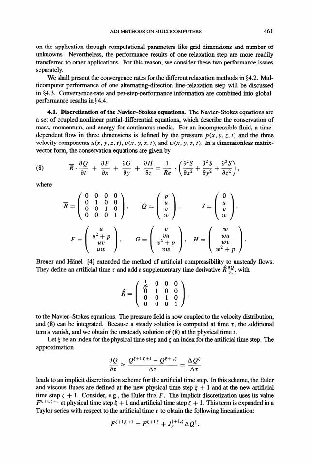
4.1. Discretization of the Navier-Stokes equations. The Navier-Stokes equations area set of coupled nonlinear partial-differential equations, which describe the conservation ofmass, momentum, and energy for continuous media. For an incompressible fluid, a time-dependent flow in three dimensions is defined by the pressure p(x, y, z, t) and the threevelocity components u(x, y, z, t), v(x, y, z, t), and w(x, y, z, t). In a dimensionless matrix-vector form, the conservation equations are given by

(8)

where

0 1 0 0 up

u0 0 1 0 Q-- S=

V 1)

0 0 0 1 w w

vuH

wuF u2 + p G1)2 + PUV WU

uw vw w2 + p

Breuer and H/inel [4] extended the method of artificial compressibility to unsteady flows.They define an artificial time r and add a supplementary time derivative/ -r, with

,--r 0 0 0r0 1 0 0R=0 0 1 00 0 0 1

to the Navier-Stokes equations. The pressure field is now coupled to the velocity distribution,and (8) can be integrated. Because a steady solution is computed at time r, the additionalterms vanish, and we obtain the unsteady solution of (8) at the physical time t.

Let be an index for the physical time step and an index for the artificial time step. Theapproximation

OQ Q+1,+1 Q+1, AQOr Ar Ar

leads to an implicit discretization scheme for the artificial time step. In this scheme, the Eulerand viscous fluxes are defined at the new physical time step + 1 and at the new artificialtime step ( + 1. Consider, e.g., the Euler flux F. The implicit discretization uses its valueF+1,(+1 at physical time step / 1 and artificial time step ( / 1. This term is expanded in aTaylor series with respect to the artificial time r to obtain the following linearization:

F+I,(+I F+I,( + JF+1’ AQ.

462 JIRN HOFHAUS AND ERIC E VAN DE VELDE

OFHere, JF is the Jacobian matrix of the Euler flux F with respect to Q, say JF --.resulting discrete system of equationsis given by

(9) LHS. AQ RHS.

The

The right-hand side contains the expressions that arise from the discretization ofthe derivativesin (8) using a high-order upwind scheme for the convective terms, central differences for thediffusive terms, and a second-order discretization for the physical time t. The left-hand sidecontains first-order spatial derivatives of the Jacobian matrices.

Because the left-hand side terms in (9) vanish for the exact solution vector Q, the discretesolution has the order of accuracy of the right-hand side. The numerical advantage is that thespatial discretization of the Jacobian matrices has no influence on the order of accuracy of thesolution. Therefore, we have gained some flexibility in choosing a discretization ofLHS. Thisflexibility is used to improve the diagonal dominance of the coefficient matrix and to increasethe size of the time step.

Although central differences would be the most straightforward choice, they do not addterms to the main diagonal of the coefficient matrix. That is why we use a first-order upwindformulation combined with a matrix-splitting technique: after splitting the Jacobian matricesinto positive and negative parts, forward differences are applied to the positive parts andbackward differences to the negative parts. Consider, e.g., the Jacobian matrix JF. This 4 x 4matrix is diagonalized such that

JF MAM-1,

where M is the matrix of eigenvectors of JF, and A is the diagonal matrix containing theeigenvalues of JF on its diagonal. Let

A=A++A-,where A+ and A- contain, respectively, the positive and negative eigenvalues. After trans-forming back to the Jacobian JF, we obtain the splitting

JF MA+M-1 + MA-M-1 J + J.The spatial derivatives in J- and J/ are discretized, respectively, with forward and backwarddifferences. This method tends to increase the diagonal entries of the coefficient matrix, andthe resulting system of equations can be solved with a line-relaxation method. For furtherdetails and for a validation of the above scheme, refer to Breuer [3] and Breuer and H/inel [4].

Every solution component consists of four elements: the pressure and the three velocitycomponents. Hence, when applying the methods described in 3, the system (3) becomes ablock-tridiagonal system, the coefficients am, bm, and Cm are 4 x 4 matrices, and the right-hand side terms dm are vectors consisting of four components. It follows that the discretizedNavier-Stokes equations require muchmore arithmetic per grid point than, e.g., the discretizedPoisson equation.

All computations of this paper use the above method to simulate the flow of an isolatedslender vortex embedded in an axial flow. The scientific interest in this tlow is the study ofthe phenomenon of a bursting vortex or vortex breakdown. Although the initial conditions areaxially symmetric, the flow is fully three-dimensional after vortex breakdown. The boundaryconditions in the outflow plane and on the lateral boundaries are extrapolated from the case ofa free vortex. At the outflow plane, a nonreflecting boundary condition simulates undisturbedvortical flow through the boundary. At the lateral boundaries, the pressure is imposed such


FIG. 3. Experimental and numericalflow visualization of bubble-type vortex breakdown: top picture showsexperimental streaklines and bottom picture shows numerical streaklines.

that the bursted part of the vortex lies well within the domain of integration. Breuer [3] givescomplete details on the initial and on the boundary conditions required to simulate this flow.

Figure 3 compares a numerical simulation and an experiment of Althaus et al. 1]. Usinga Reynolds number based on the radius of the vortex core as length scale and the mean axialvelocity as velocity scale, both cases have a Reynolds number of 500. Our simulation uses a32 x 32 64 rectangular grid with the z-direction being the axial coordinate. The physical timestep is 0.3, and the artificial time step is 100. Althaus et al. 1] perform a detailed comparisonof numerical and experimental results. It is this computation that we use to evaluate theperformance of all our codes.

Depending on the orientation of the relaxation line, we have to solve 32 64 2048systems of 32 blocks or 32 32 1024 systems of 64 blocks of size 4 4. Our challenge isto make effective use of all 512 computing nodes of the Delta to solve the block-tridiagonalsystems ofthis moderate size. As discussed in 2, we use a P Q R process grid. Preliminarytests, which we do not report, showed that three-dimensional grid distributions outperformone- and two-dimensional grid distributions with P 1 and/or Q 1, in spite of the fact thatthe latter can use efficient sequential tridiagonal solvers in at least one direction. This mayseem somewhat counterintuitive. Given a certain number of nodes, choosing P 1 leads tohigher values for Q and/or R. The fact that x-line,relaxation steps are very efficient whenP 1 is offset by the increased load imbalance and the decreased efficiency in the otherdirections. Therefore, we always use a process grid with P + Q + R; see Table 1. In all ourcomputations, each process is mapped to a separate node of the multicomputer.

The experiments of this section were performed on the Intel Touchstone Delta [5], whichconsists of an ensemble of 512 computing nodes connected in a two-dimensional mesh. Thecomputational engine of each node is an Intel i860 processor with an advertised peak perfor-

464 JRN HOFHAUS AND ERIC E VAN DE VELDE

10-2

10-3

Residual 10-4

10-5

10-6

8 processes\ 64 processes

512 processes

0 50 100 150 200 250Number of line-relaxation steps

FI6. 4. Maximal residual as a function of the number ofmodified half-Gauss-Seidel line-relaxation stepsforthree different process grids.

TABLEProcess grids used in our computational tests.

TotalNumber

48163264128256512

Number of processes in

x-direction (p) .Y.-dire.ctin (Q) I.. z-directin.(R)4

2 2 22 2 4

4 4 44 4 84 4 168 8 8

mance of 60 double-precision MFLOPS. Each node has a local memory of 16 MB. On theDelta, our standard problem needs a minimum offour nodes because ofmemory requirements.

4.2. Convergence of relaxation methods.

4.2.1. Modified half-Gauss-Seidel line relaxation. The modified half-Gauss-Seidelline relaxation uses the updated unknowns of the previously computed plane except at processboundaries; see 2. The convergence rate of the modified method is dependent on the numberof processes and on the choice of process boundaries, because they determine the matrixsplitting underlying the relaxation method. Figure 4 shows the residual as a function of thenumber ofrelaxations for some ofthe partitions ofTable 1. Although the convergence dependson the partition, all computations achieve the required residual of 10-5 within approximatelythe same number of iteration steps.

4.2.2. Jacobi line relaxation. In the case of Jacobi line relaxation, all relaxation linesmay be computed simultaneously. The convergence rate of the Jacobi line relaxation does notdepend on the number of processes. Note that the modified half-Gauss-Seidel line relaxationturns into the Jacobi line relaxation when the number of processes is equal to the number ofgrid planes.


Residual

10-2

10-3

10-4

10-5

10-60 50

Jacobi linemodified half Gauss-Seidel line

100Number of line-relaxation steps

150 200 250

Fla. 5. Maximal residual as afunction ofthe number ofline-relaxation steps in a computation with 64 processes.

In Fig. 5, half-Gauss-Seidel and Jacobi line relaxation on the 64-node partition are com-pared. The Jacobi method needs about 10% more iteration steps to reach the required toleranceon the residual.

4.2.3. Red-Black line relaxation. Like the Jacobi line relaxation, the convergence rateof the Gauss-Seidel line relaxation with red-black ordering does not depend on the numberof processes. We obtained a test program for the red-black line relaxation easily by splittingthe Jacobi relaxation into the two steps explained in 2 and changing the step width of theinner loops to two. After the first step, the updated unknowns have to be exchanged betweenthe processes. Besides the required additional communication, there is a loss of performance,because the inner loops can no longer be vectorized.

For our application, there is no observable difference in the convergence rate between thered-black and the Jacobi line iteration. The red-black line relaxation is, therefore, not a viablealternative to the modified half-Gauss-Seidel line method and, because of the communicationand vectorization losses, its global performance is worse than the Jacobi line relaxation.

4.2.4. Segment relaxation. The segment relaxation computes relaxation lines inter-rupted by the process boundaries. Efficiency and applicability of this method depend onthe convergence rate of the resulting iteration. Consider a segment-relaxation step in onedirection with M grid points distributed over P processes, and let

MP

be the number of local grid points. For I M, we obtain a sequential line relaxation, whilea Jacobi point relaxation results if I 1.

We implemented an alternating-direction segment relaxation and plot the residual as afunction of the number of relaxation steps for a 256- and a 512-node partition in Fig. 6. Theplot shows that the relaxation fails to converge for the unbalanced 4 x 4 x 16 partition. The8 x 8 x 8 partition needs about 20% more iteration steps than the modified half-Gauss-Seidelline relaxation.

We observed a nonconverging iteration even for the 2 x 2 x 8 partition. We conclude thatsegment relaxation is not suitable, because robustness of the algorithm cannot be guaranteed.

466 JORN HOFHAUS AND ERIC F. VAN DE VELDE

Residual

10-2

modified half Gauss-Seidel linesegment on 256 processes

10-3 segment on 512 processes

10-4

10-5

10-60 50 i00 150 200 250

Number of line-relaxation steps

FIG. 6. Maximal residual as afunction ofthe number ofline-relaxation stepsforsegment relaxation and modifiedhalf-Gauss-Seidel line relaxation.

Although we achieve convergence when using all nodes on the Delta, it is uncertain whetherthe code would converge on a larger configuration of the same hardware. We consider thisnonrobust behavior unacceptable.

4.2.5. Iterative block-tridiagonal solver. The modified half-Gauss-Seidel line relax-ation of 4.2.1 can also be implemented using the concurrent iterative block-tridiagonal solverof3.3. Because this methodsolves the system (3) only approximately, one should consider theeffect of less-accurate block-tridiagonal solvers on the convergence rate of the line-relaxationmethod.

In Fig. 7, we examine the impact on the number of line-relaxation steps of using theiterative solver with six block-tridiagonal iteration steps. (The rationale for using six iterationsteps is discussed in 4.3.6.) The curves for the exact and iterative solvers show the sameprogress, and the required residual of 10-5 is reached almost within the same relaxation step.

With an increasing number ofprocesses, the initial guess (7) gets worse, andmore couplingcoefficients are set equal to zero to obtain the tridiagonal-iteration matrix. The partition,therefore, has an impact on the convergence rate. Figure 8 compares three different partitions.Up to 256 processes, the curves virtually coincide. The computation with 512 nodes requiresonly a few additional line-relaxation steps to converge.

4.3. Performance of one alternating-direction line-relaxation step. In this section,we shall compare the multicomputer performance of one alternating-direction line-relaxationstep, i.e., one line relaxation in each spatial direction. To obtain a dimensionless efficiencyfor a multicomputer program, one must relate the execution time to a meaningful referencetime. In principle, this reference time must be the best execution time possible on one nodeof the same multicomputer. In reality, one must settle for the sequential-execution time ofa reasonable but not necessarily the best sequential program. For us, even the reasonablesequential time is impossible, because our problem requires too much memory to solve on onenode. We defined a fictitious reference time in the following manner. To obtain a sequentialtime for the relaxation in the x-direction, we distribute the grid only in the y- and z-directionsover the processes. Subsequently, the concurrent-execution time for this partition is then mul-tiplied by the number of processes. We repeat this method for the y- and z-directions. Our


Residual

10-2

10-3

10-4

10-5

10-60 50

exact solveriterative solver

100 150 200 250Number of line-relaxation steps

FIG. 7. Maximal residual as a function of the number of line-relaxation steps when using the exact and theiterative block-tridiagonal solver to implement modified half-Gauss-Seidel line relaxation with 64 processes.

10-3

Residual 10-4

10-5

10-6

8 processes64 processes

512 processes

0 50 100 150 200 250Number of line-relaxation steps

FIG. 8. Maximal residual as afunction ofthe number ofline-relaxation steps to examine impact ofprocess gridson the iterative block-tridiagonal solver.

sequential-execution time for the alternating-direction line relaxation is the sum of these threeterms. With process boundaries that are parallel to the relaxation lines, the block-tridiagonalsystems can be solved by sequential LU-decomposition, which is the optimal procedure forsequential computations.

The same reference time is used for all methods, such that the efficiency results can becompared directly. The efficiency Op of a P-node computation is the ratio

(reference sequential time)P (execution time of the P-node program)

We shall compare the multicomputer performance by means of two different kinds of plots.The first kind plots the efficiency r/, as a function of the number of nodes, and the second


plots the execution time Tp in seconds as a function of the number of nodes. In both plots, alogarithmic scale is used for the number of nodes. In the execution-time plot, we also use alogarithmic scale for the second axis such that the line of linear speedup has slope 1. (Theslope is distorted, however, because different scaling factors are used for the horizontal andvertical axes.)

The increased computational requirements of the discrete Navier-Stokes equations over,e.g., the discrete Poisson equation actually results in a more efficient computation, becausemore arithmetic occurs for the same number of messages. Although the messages are longerfor the discrete Navier-Stokes equations, the latency usually dominates the communicationtime, and the length of the messages is less important than the number of messages.

4.3.1. Pipelining. In 3.1, we described a pipelining method for the sequential LU-decomposition. This makes sense if the number of processes is small compared with thenumber of unknowns per block-tridiagonal system [8]. This method, compared with all othermethods we implemented, has the lowest floating-point operation count and requires the leastamount of communication. However, it is less concurrent than some other methods becauseof load imbalance. The pipelining implements the Jacobi line relaxation.

Figure 9 shows the performance of the pipelining algorithm. As expected, the algorithmshows good efficiency for a small number of processes. However, for larger numbers ofprocesses, the startup time required for all processes to participate in the computation causesa progressive loss of efficiency.

4.3.2. Recursive doubling. A concurrent implementation of the modified half-Gauss-Seidel line relaxation with the recursive-doubling algorithm for block-tridiagonal systemsrequires more arithmetic and more communication than the pipelining method, but offershigher concurrency. The recursive-doubling computations in the execution-time plot of Fig.10 lie on a line that is almost parallel to the line of linear speedup. These lines are parallel andthe efficiency is constant as a function of the number of nodes, because the communicationoverhead plays only a secondary role in computations with up to 512 nodes. The verticaldistance between these two lines can be related to the arithmetic overhead, which is mainlyresponsible for the disappointing efficiency of about 15%.

4.3.3. Cyclic reduction. The cyclic-reduction algorithm is based on the same reductionprocedure as recursive doubling and is also an implementation of the half-Gauss-Seidel linerelaxation. This method needs less arithmetic, but additional communication for the back-substitution. Whereas the local part of the cyclic reduction shows a good load balance, thenumber of processes that participate during the global part halves after each reduction step.Both facts lead to a significant loss of efficiency for large numbers of processes (Fig. 10).However, cyclic reduction always beats recursive doubling. It beats the pipelining method forcomputations with all available nodes (see also Table 2).

For the back-substitution, the cyclic-reduction algorithm must store the entries of thecoefficient matrix T and the right-hand side terms in (3), which change after each reductionstep. The additional memory made a run on four nodes impossible.

The dips in the efficiency curves for 32 and 256 processes occur, because we double thepartitions in the x- and y-directions (see Table 1). In these cases, the z-line-relaxation stepsare inefficient compared to the next larger partition (2 x 2 x 8 4 x 4 4 and 4 x 4 16

8 8 x 8, respectively).

4.3.4. Partition method. When modified half-Gauss-Seidel line relaxation is imple-mented by means of Wang’s partition method, we realize an improved efficiency comparedwith the cyclic-reduction algorithm; compare Figs.. 10 and 11. We examined in detail exe-cution profiles of the z-line relaxation with a 1 x 1 x 8 process grid. In this case, already


0.8

0.6

0.4

0.2

8 16 32 64 128 256 512Number of nodes

100

10Tp

[sec]

pipelininglinear speedup

2 4 8 16 32 64 128 256 512Number of nodes

FIG. 9. Efficiency and execution time ofthe pipelining algorithm.

about 40% of the execution time was needed for solving the reduced system computed in thefirst part of Wang’s partition method. This step is communication intensive and becomes evenmore so when the number of processes is increased further. It is this part of the computationthat is responsible for the gradual loss of efficiency as the number of processes is increased.

4.3.5. Divide and conquer. The performance of the divide-and-conquer algorithm ap-plied to the modified half-Gauss-Seidel line-relaxation method is given in Fig. 11. Like thepartition method, divide and conquer reduces the size of the tridiagonal systems down to oneblock of equations per process.

The communication needed for the solution of the reduced system, obtained again withrecursive doubling, decreases the efficiency of larger partitions in our application. The per-formance as a function of the number of processes is almost identical to that of the partition


P

0.8

0.6

0.4

0.2

recursive doubling --cyclic reduction -+--

4 8 16 32 64 128 256 512Number of nodes

100

10Tp

[sec]

recursive doublingcyclic reduction --linear speedup

2 4 8 16 32 64 128 256 512Number of nodes

FI. 10. Efficiency and execution time ofrecursive doubling and cyclic reduction.

TABLE 2Execution times until convergence on 512 nodes.

Block-tridiagonal Execution timesolver in seconds

Iteration method 10.12Partition method 11.08

Divide and conquer 12.31Cyclicreduction 12.44

Pipelining 14.96Recursive doubling 39.64


0.8

0.6

0.4

0.2

partition methoddivide and conquer -+--

8 16 32 64 128 256 512Number of nodes

100

10Tp

[sec]

linear speedup

partition methoddivide and conquer -+--

2 4 8 16 32 64 128 256 512Number of nodes

FIG. 11. Efficiency and execution time ofthe partition and the divide-and-conquer method

method. The divide-and-conquer algorithm outperforms the partitioning method on smallerprocess grids.

4.3.6. Iterative block-tridiagonal solver. With the iterative block-tridiagonal solver, weimplemented the modified half-Gauss-Seidel line relaxation. Because the iteration methodsolves the block-tridiagonal systems approximately, the accuracy requirements are a decisivedeterminant for the performance of the iteration method. In principle, it would be possible toiterate until a certain criterion is satisfied, e.g.,

(10) I (/z) / (/z-1)l E,

where e is a certain tolerance. If e is small, the iterative solver is numerically equivalent to adirect solver. However, if e is large, the error on the solution of the tridiagonal system may

472 J)RN HOFHAUS AND ERIC E VAN DE VELDE

have an impact on the convergence rate of the line relaxation. The size of e in (10), therefore,not only determines the number of block-tridiagonal iteration steps, but also the number ofline-relaxation steps.

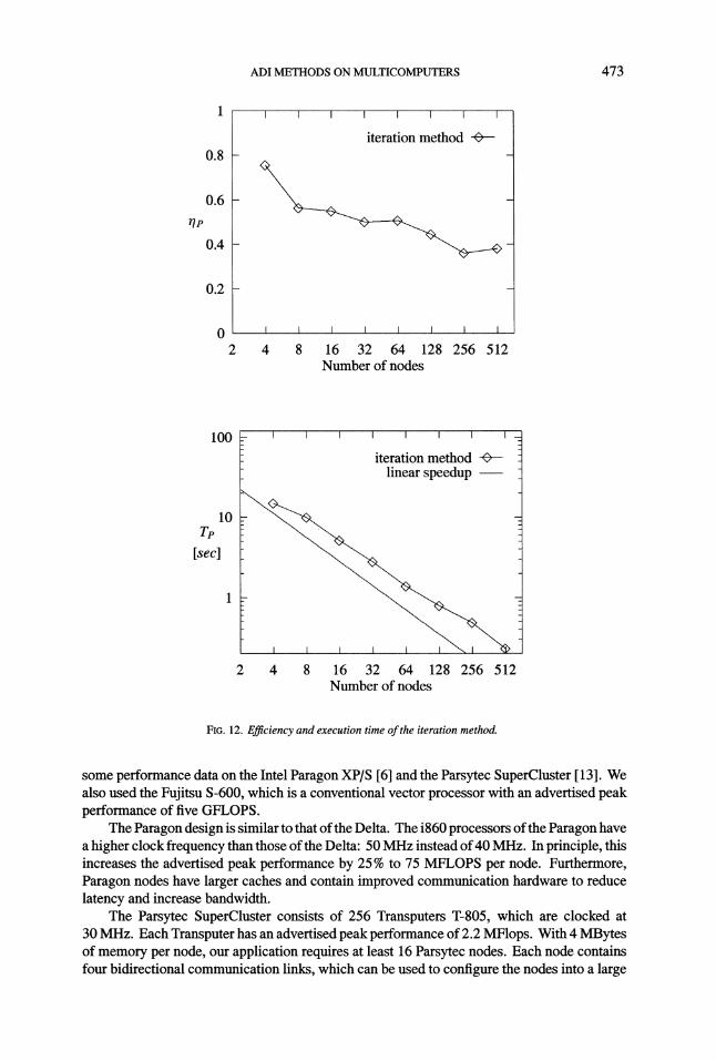
In a multicomputer computation, error-adaptive strategies like those suggested by (10)add significant costs that are difficult to recoup by the expected reduction in the number ofiteration steps: computing error estimates is expensive, because they require global commu-nication. Therefore, (10) is not used in our final computation. Instead, we are using a fixednumber of block-tridiagonal iteration steps. We found that this is more efficient, while highlyreliable if the number of block-tridiagonal iteration steps is sufficiently large. To determinean appropriate number, we performed a sequence of experiments on a 1 1 8 process grid.In (10), we set e 10-6, which is one order of magnitude below the requested residual ofthe global relaxation. We found that six iterations were always sufficient to reach the requiredaccuracy if the initial guess t of (7) was used. The performance results shown in Fig. 12were all measured with the number of block-tridiagonal iteration steps set equal to 6. Withmore than 32 processes, the algorithm is more efficient than the partition method and moreefficient than the divide-and-conquer technique. With 256 processes, the performance is betterthan any other concurrent algorithm we implemented.

It was already shown in 4.2.5 that, with six block-tridiagonal iteration steps, there wasvirtually no difference in the number of line-relaxation steps between the iterative and theexact block-tridiagonal solver. Line-relaxation steps based on either solver are, therefore,practically equivalent. It is possible to reduce the number of block-tridiagonal iteration stepsbelow six. However, the resulting line-relaxation method is no longer equivalent with theoriginal method and may require a larger number of line-relaxation steps. On the other hand,each line-relaxation step may be considerably less expensive. We did not pursue this possibilityof trading off the accuracy of the block-tridiagonal solver with the convergence rate of theline-relaxation method. However, segment relaxation is equivalent to line relaxation with oneiteration step of the iterative block-tridiagonal solver. Considering the robustness problemsof segment relaxation, at least two block-tridiagonal iteration steps are needed.

4.4. Global performance. The interesting performance of a program is, of course, theexecution time until convergence within tolerance. In Fig. 13, we compare this time forthe Jacobi line-relaxation method implemented with pipelining and for the modified half-Gauss-Seidel line relaxation implemented with the partition method and with the iterativeblock-tridiagonal solver. Here, we focus only on the execution time needed for the relaxationroutines. To obtain the actual time to solve the Navier-Stokes equations, we must add to thisthe time for the computation of the right-hand side terms and the boundary conditions, whichare independent of the solution procedure.

The better performance of the iterative block-tridiagonal solver for computations withmore than 256 processes is partially offset by the required additional relaxation-iterationsteps; see 4.2.5. The convergence losses of the Jacobi line relaxation (4.2.2) deteriorate theperformance of the pipelining algorithm. The execution times until convergence on 512 nodesfor all implementations are given in Table 2. The modified half-Gauss-Seidel line relaxationimplemented with the iterative block-tridiagonal solver clearly beats all competitors. Aspointed out before, there are several techniques that could improve its performance evenfurther. Most importantly, the fastest method is also, by far, the easiest to implement.

5. Computer dependence. The execution time of a program is, by its very nature, acomputer-dependent characteristic. One must, therefore, always question whether or not par-ticular performance results for a set of algorithms obtained on one computer carry over to othercomputers. Although not our main concern here, comparative performance studies can alsobe used for computer-evaluation purposes. In a preliminary comparative study, we obtained


0.8

0.6

0.4

0.2

iteration method

4 8 16 32 64 128 256 512Number of nodes

100

10Te

[sec]

linear speedupiteration method

2 4 8 16 32 64 128 256 512Number of nodes

FIG. 12. Efficiency and execution time ofthe iteration method.

some performance data on the Intel Paragon XP/S [6] and the Parsytec SuperCluster 13]. Wealso used the Fujitsu S-600, which is a conventional vector processor with an advertised peakperformance of five GFLOPS.

The Paragon design is similar to that ofthe Delta. The i860 processors ofthe Paragon havea higher clock frequency than those ofthe Delta: 50 MHz instead of40 MHz. In principle, thisincreases the advertised peak performance by 25% to 75 MFLOPS per node. Furthermore,Paragon nodes have larger caches and contain improved communication hardware to reducelatency and increase bandwidth.

The Parsytec SuperCluster consists of 256 Transputers T-805, which are clocked at30 MHz. Each Transputer has an advertised peak performance of 2.2 MFlops. With 4 MBytesof memory per node, our application requires at least 16 Parsytec nodes. Each node containsfour bidirectional communication links, which can be used to configure the nodes into a large


time [sec

1000

100

10

pipelining -@--partition method --+---

4 8 16 32 64 128 256 512Number of nodes

FIG. 13. Execution time until residual < 10-5.

variety of network topologies. The floating-point performance of the Transputer is consider-ably less than that of a Paragon or a Delta node. However, the Parsytec has an excellent ratioof communication versus arithmetic time.

In Figs. 14, 15, and 16, the execution time ofone alternating-direction line-relaxation stepis displayed as a function of the number of nodes. Figure 14 considers Jacobi line relaxationimplemented using the pipelined block-tridiagonal solver on the Delta, Paragon, and Parsytec.Figures 15 and 16 display execution times obtained with modified half-Gauss-Seidel linerelaxation. Figure 15 is for the program based on the concurrent iterative block-tridiagonalsolver, and Figure 16 for the program that uses the partition method to solve the block-tridiagonal systems concurrently. In these three figures, the lines of linear speedup are basedon a sequential-execution time obtained for the Delta as explained in 4.3. The lines of linearspeedup for Paragon and Parsytec are parallel to this line, but are not displayed to avoidcrowding the figures; Parsytec efficiency is compared with Delta efficiency in Fig. 17.

In the execution-time plots, the Parsytec computations lie on a line that is almost parallelto the line of linear speedup. This is most pronounced for the method based on the iterativeblock-tridiagonal solver. This is an indication that almost all overhead on the Parsytec is due tothe increased operation count of the concurrent computations and not to communication. Thisis confirmed in the efficiency plots of Fig. 17, which displays the efficiencies as a function ofthe number of nodes. (Efficiencies are computed using the sequential-execution time on thecomputer of the concurrent computation.) The iteration method on the Parsytec has a constantefficiency of about 40%, which indicates that communication overhead is negligible. When

2.5 times slower thanexecuted on one node, the concurrent Parsytec program is aboutthe sequential Parsytec program. However, the concurrent program speeds up linearly.

The pipelining method does not have a constant efficiency on the Parsytec. However,its decrease in efficiency is much less pronounced than on the Delta: communication andload-imbalance effects are not as important on the Parsytec as on the Delta. This is, of course,easily explained by the smaller communication-arithmetic ratio of the Parsytec.

Because of the low floating-point-operation count of the pipelining method and the highcommunication efficiency of the Parsytec, pipelining remains the fastest algorithm for up tothe maximum available number ofnodes (256). However, extrapolating Fig. 17, we expect that


time [sec

100

10

Intel Touchstone Delta-.,_ Parsytec SC-256 --+--Intel Paragon XP/S

_eedup

4 8 16 32 64 128 256 512Number of nodes

FIG. 14. Execution time ofthe pipelining method.

time [sec

100

10

Intel Touchstone Delta --Parsytec SC-256 -+--edup

8 16 32 64 128 256 512Number of nodes

15. Execution time ofthe iteration method.

the iteration method will perform better than the pipelining method on Parsytec-like computerswith more than 512 nodes.

For our computations, the Delta is about 10-13 times faster than the Parsytec. Basedon the advertised peak performance of their nodes, the Delta should be about 30 times fasterthan the Parsytec. The speed difference between Parsytec and Delta is smaller for fine-graincomputations, because the Parsytec is a more efficient computer. The higher efficiency is notenough, however, to close the speed gap with the Delta.

As mentioned before, our code solves the Navier-Stokes equations to simulate time-dependent, incompressible, and unsteady flows. Table 3 displays typical execution times toobtain useful fluid-dynamical results. These require about 1000 physical time steps, and eachtime step requires many line-relaxation steps. These execution times also include all othercomputations that surround the actual alternating-direction line-relaxation iteration. The most

476 JORN HOFHAUS AND ERIC E VAN DE VELDE

time [sec

100

10

Intel Touchstone Delta -0--". Par.sytec SC-25 -+--

-!2 4 8 16 32 64 128 256 512

Number of nodes

FIG. 16. Execution time ofthe partition method.

TABLE 3Typical execution timesfor the production offluid-dynamical results.

Execution time in hours onComputer 8 nodes 64 nodes 256 nodes

Intel Paragon XP/S 70.8 14.3Intel Touchstone Delta 97.2 18.2 9.1

Parsytec SC-256 23512 84.2

512 nodes

Fujitsu S-600 13.1

important factor in these periferal-but-necessary computations is the evaluation ofthe boundaryconditions. For our application, the Fujitsu S-600 is equivalent to about 64 Paragon nodes.Whereas an individual line-relaxation step is almost four times faster on 256 Delta nodes thanon 64 Delta nodes, only a factor of two is obta’.med in the global computation. This is dueto the increasing influence of the evaluation of the boundary conditions, which introducessignificant load imbalance in finer-grain computations.

6. Summary. We presented several concurrent methods for solving sets ofblock-tridiag-onal systems on a rectangular grid. Previous studies concentrated on computations of veryhigh granularity, which we found to be unrealistically high for our application. Therefore,we tested several methods to solve a larger number of smaller systems. All methods showa significant speedup on test runs up to 512 processes. On the Touchstone Delta, the bestefficiency achieved was about 40%.

Although problem sizes will significantly increase beyond the size ofthe problem studiedin this paper, we believe that granularity will remain of the same order of magnitude or mighteven decrease significantly. For most problems, the total amount of arithmetic increases fasterthan linearly with the total amount of data (which itself is proportional to the number ofunknowns). To keep the total execution time reasonable, one should use a number of nodesproportional to the total amount of arithmetic. Hence, the amount of data per node (thegranularity) is likely to decrease. There is also a numerical reason why fine-grain concurrencywill become increasingly important. To improve the convergence rate, one could consider


Delta

P

0.8

pipelining

16 32 64 128 256 512Number of nodes

Parsytec

0.8

0.6

0.4

0.2

pipeliningiteration method -+---_

16 32 64 128 256Number of nodes

FIG. 17. Efficiency ofpipelining and iteration methods on the Delta and Parsytec multicomputers.

using line-relaxation methods as smoothers in a nonlinear multigrid method. The coarserlevels, however, quickly require computations of fine granularity.

Block-tridiagonal solvers that are efficient for fine-grain computations are difficult toimplement. Nevertheless, it is possible to achieve significant execution-time improvementsthrough the use of relatively fine-grain concurrency. A significant simplification for futureendeavors is that our best results were obtained with the iterative block-tridiagonal solver,which is, from an algorithmic point of view, the simplest.

REFERENCES

1] W. ALTHAUS, E. KRAUSE, J. HOFHAUS, AND M. WEIMER, Bubble- andspiral-type breakdown ofslender vortices,Exp. Thermal Fluid Sci., (1995), to appear.

478 JORN HOFHAUS AND ERIC F. VAN DE VELDE

[2] S. BONDELI, Divide and conquer: A parallel algorithmfor the solution ofa tridiagonal system ofequations,Parallel Comput., 17 (1991), pp. 419-434.

[3] M. BREUER, Numerische Liisung der Navier-Stokes Gleichungen ffir dreidimensionale inkompressible insta-tioniire Striimungen zur Simulation des Wirbelaufplatzens, Ph.D. thesis, Aerodynamisches Institut derRWTH Aachen, Germany, 1991.

[4] M. BREUERAND D. H,NEL,A dual time-stepping methodfor 3-D, viscous, incompressible vortexflows, Comput.& Fluids, 22 (1993), pp. 467-484.

[5] INTEL SUPERCOMPUTING SYSTEMS DIVISION, Touchstone Delta System User’s Guide, Beaverton, Oregon, 1991.[6] , The Intel Paragon Supercomputer--an Overview, Beaverton, Oregon, 1992.[7] A. FROMMER, Lisung linearer Gleichungssysteme auf Parallelrechnern, Vieweg-Verlag, Braunschweig,

Germany, 1990.[8] C. Ho AND S. JOHNSSON, Optimizing tridiagonal solversfor alternating direction methods on Boolean cube

multiprocessors, SIAM J. Sci. Statist. Comput., 11 (1990), pp. 563-592.[9] R. HOCKNEY,Afast and direct solution ofPoisson ’s equation using Fourier analysis, J. Assoc. Comput. Mach.,

(1965), pp. 95-113.10] R. HOCKNEY AND C. JESSHOPE, Parallel Computers, Adam Hilger, Bristol, 1981.11] E. ISAACSON AND n. KELLER, Analysis ofNumerical Methods, John Wiley and Sons, New York, 1966.[12] S. JOHNSSON, Y. SAGO, AND M. SCHULTZ, Alternating direction methods on multiprocessors, SIAM J. Sci.

Statist. Comput., 8 (1987), pp. 686-700.[13] W. JULING AND K. KREMER, The massively parallel computer system of the DFG priority research program

"flow simulation on supercomputers ", in Notes on Numerical Fluid Mechanics, Vol. 38, Vieweg-Verlag,Braunschweig, Germany, 1993.

14] A. KRECHEL, H.-J. PLUM, AND K. STOBEN, Parallelization andvectorization aspects ofthe solution oftridiagonallinear systems, Parallel Comput., 14 (1990), pp. 31-49.

15] H. STONE, An efficientparallel algorithmfor the solution ofa tridiagonal linear system ofequations, J. Assoc.Comput. Mach., 20 (1973), pp. 27-38.

[16] H. WANG, A parallel methodJbr tridiagonal equations, ACM Trans. Math. Software, 7 (1981), pp. 170-183.

z) 0(m2/3). - california institute of...

Documents