z transform - department of eehcso/ee3210_8.pdfz transform. chapter intended learning outcomes: (i)...

H. C. So Semester B 2016-2017

z Transform

Chapter Intended Learning Outcomes: (i) Represent discrete-time signals using transform (ii) Understand the relationship between transform and

discrete-time Fourier transform (iii) Understand the properties of transform (iv) Perform operations on transform and inverse

transform (v) Apply transform for analyzing linear time-invariant

systems


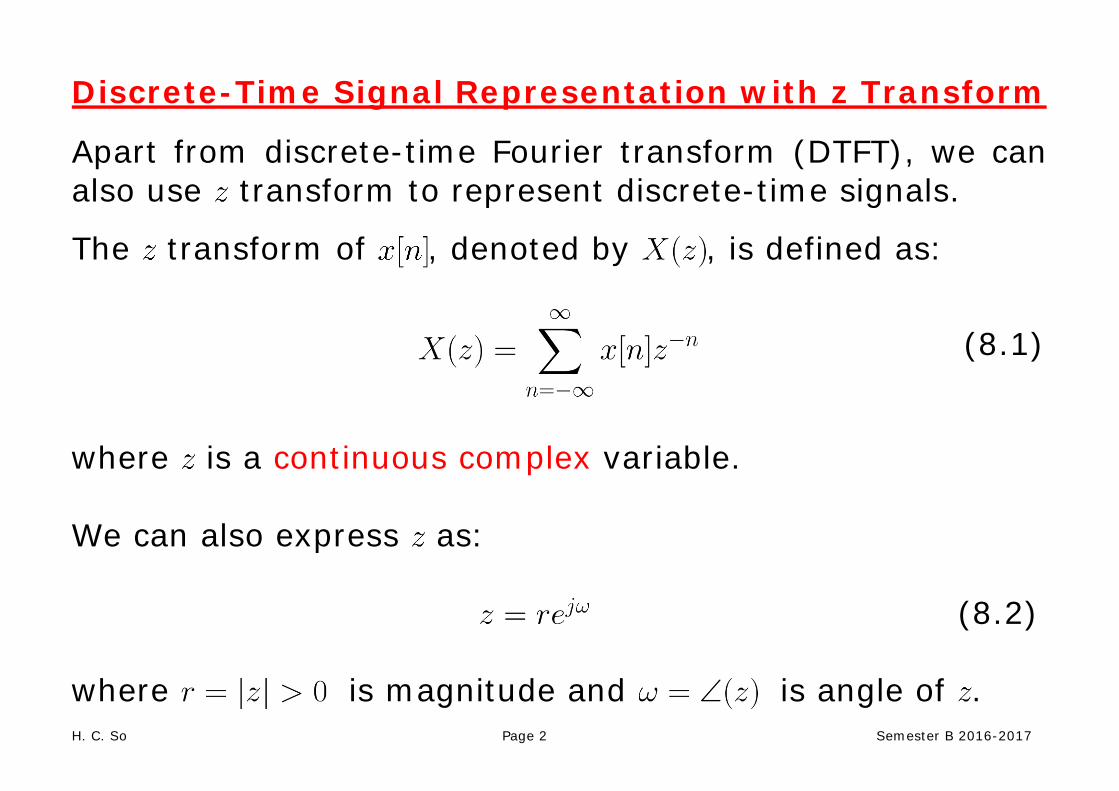
Discrete-Time Signal Representation with z Transform

Apart from discrete-time Fourier transform (DTFT), we can also use transform to represent discrete-time signals.

The transform of , denoted by , is defined as: (8.1)

where is a continuous complex variable. We can also express as: (8.2) where is magnitude and is angle of .


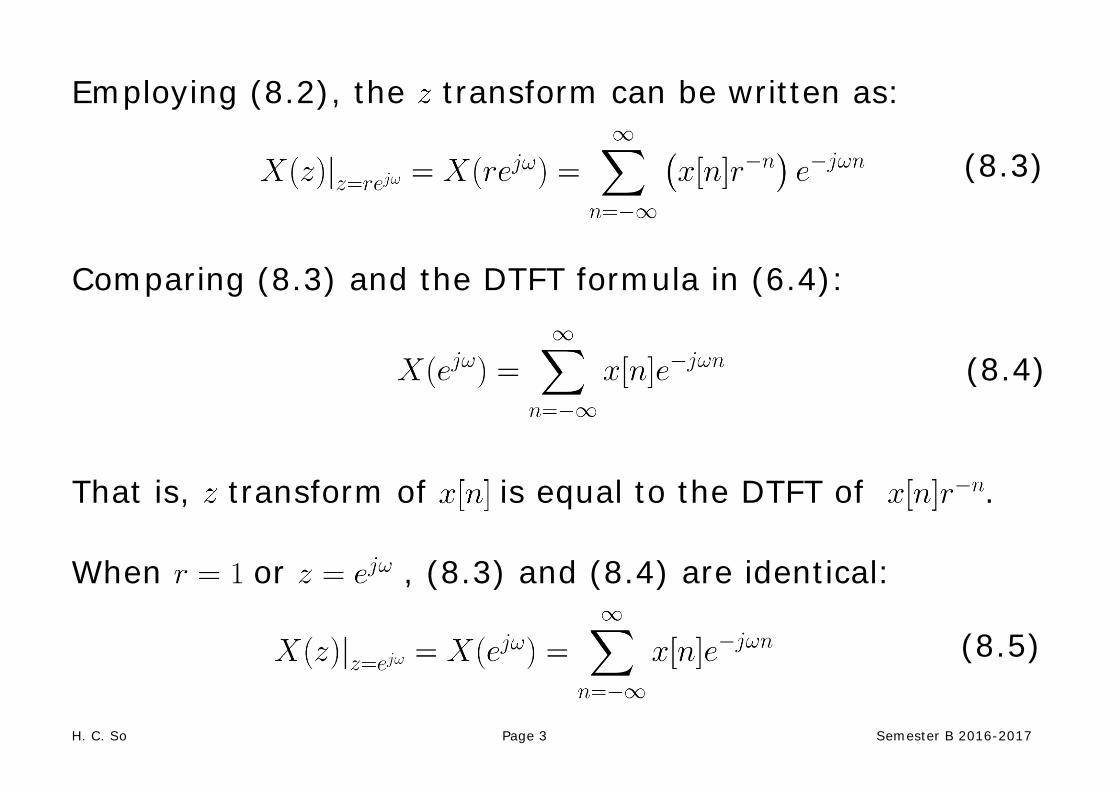
Employing (8.2), the transform can be written as:

(8.3)

Comparing (8.3) and the DTFT formula in (6.4):

(8.4)

That is, transform of is equal to the DTFT of . When or , (8.3) and (8.4) are identical:

(8.5)


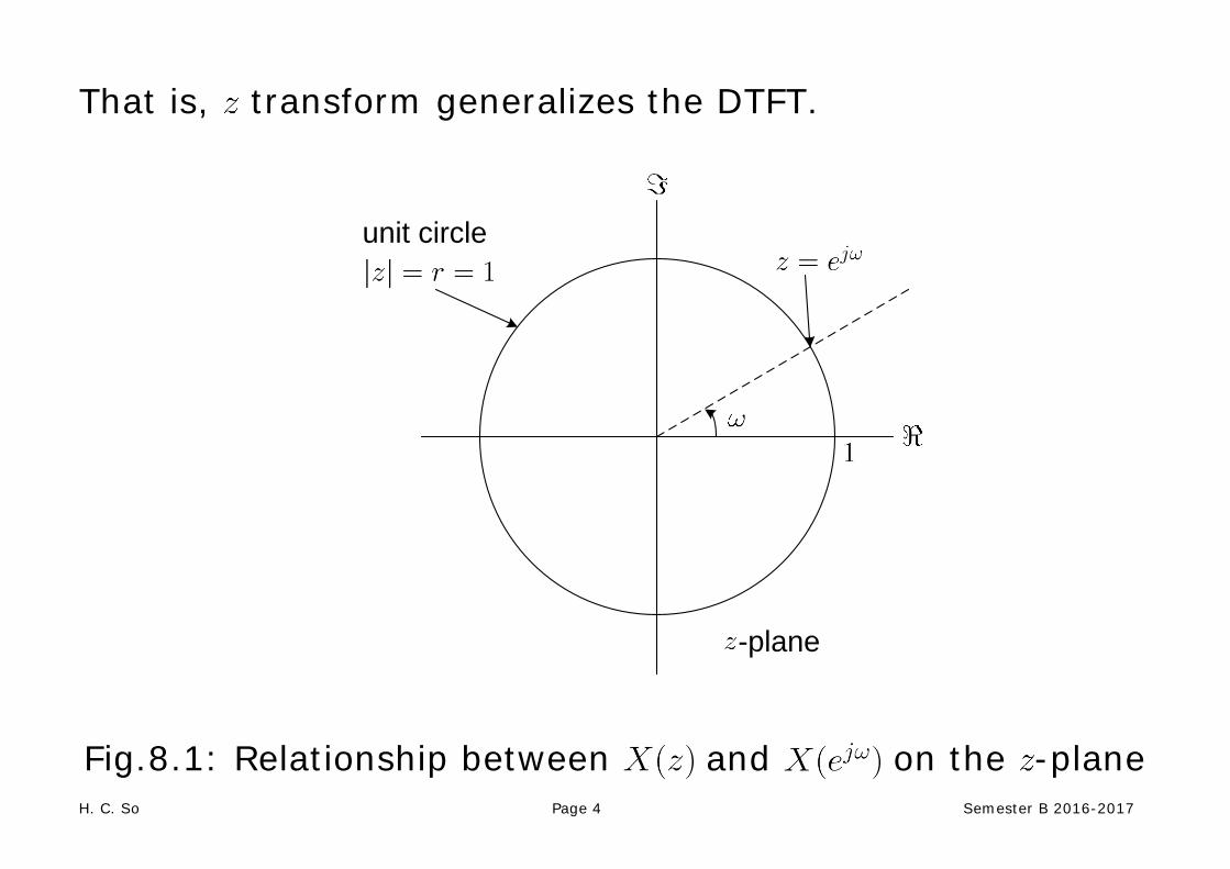
That is, transform generalizes the DTFT.

unit circle

-plane

Fig.8.1: Relationship between and on the -plane


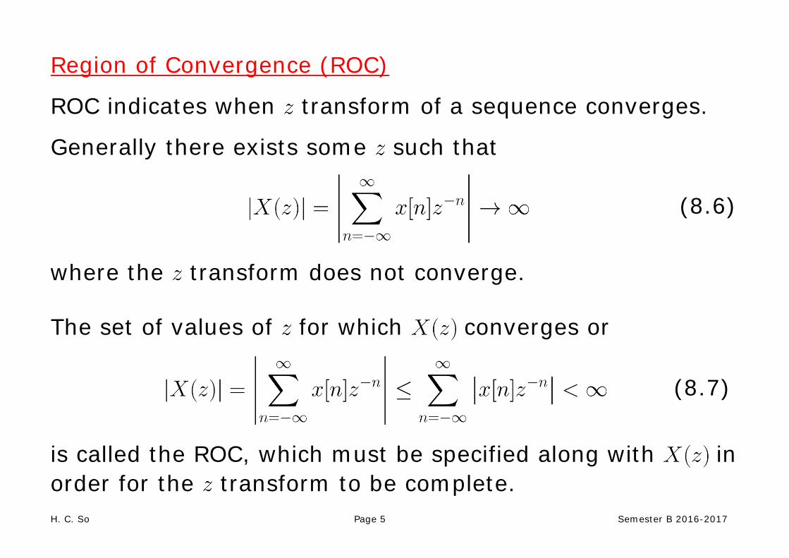
Region of Convergence (ROC)

ROC indicates when transform of a sequence converges.

Generally there exists some such that

(8.6)

where the transform does not converge. The set of values of for which converges or

(8.7)

is called the ROC, which must be specified along with in order for the transform to be complete.


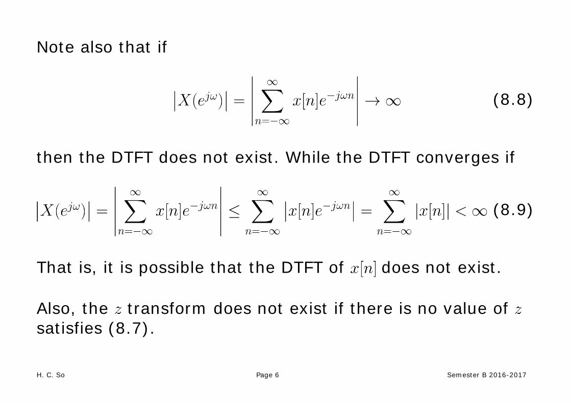
Note also that if

(8.8)

then the DTFT does not exist. While the DTFT converges if

(8.9)

That is, it is possible that the DTFT of does not exist. Also, the transform does not exist if there is no value of satisfies (8.7).


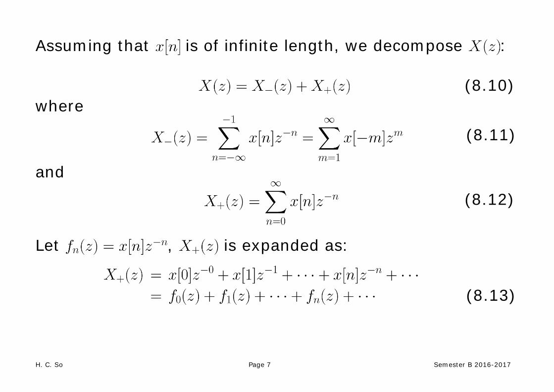
Assuming that is of infinite length, we decompose : (8.10) where

(8.11)

and

(8.12)

Let , is expanded as:

(8.13)


According to the ratio test, convergence of requires

(8.14)

Let . converges if

(8.15)

That is, the ROC for is .


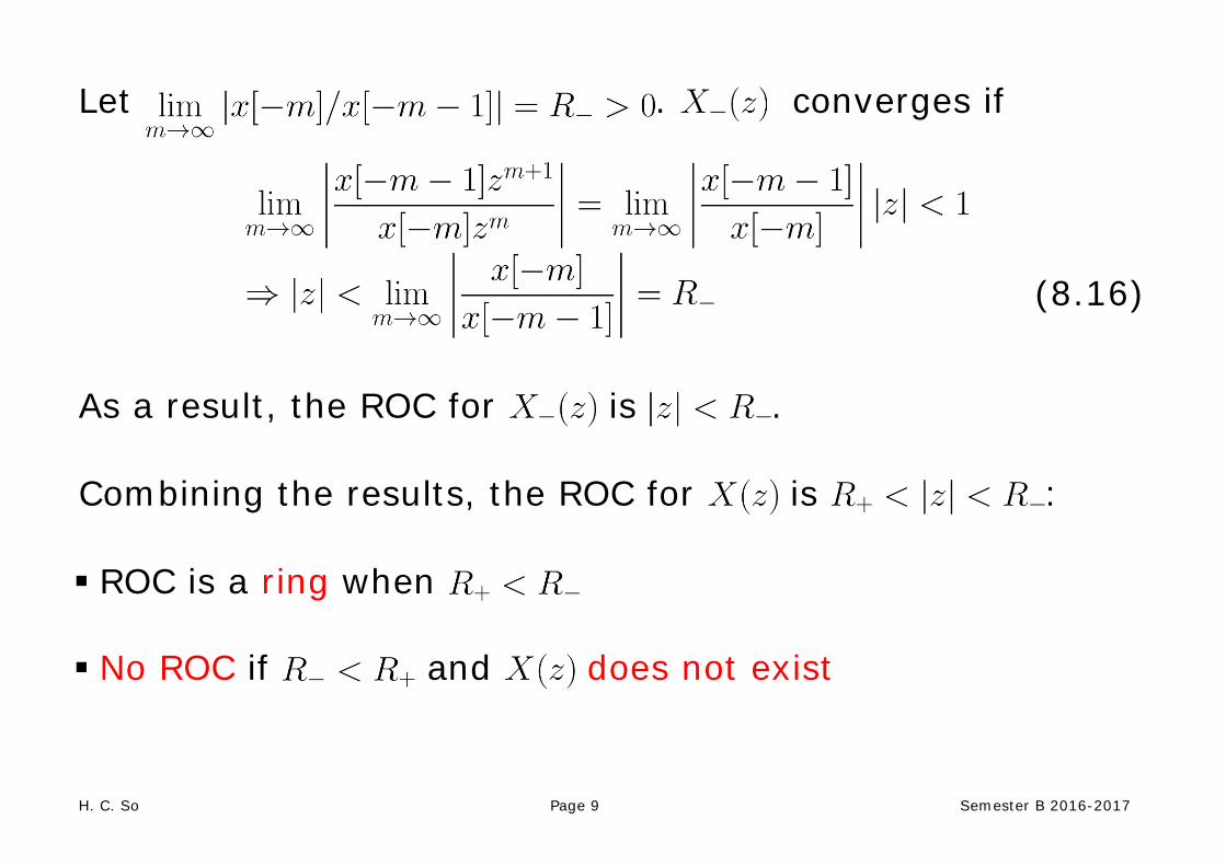
Let . converges if

(8.16)

As a result, the ROC for is . Combining the results, the ROC for is : ROC is a ring when No ROC if and does not exist


-plane-plane-plane-plane

Fig.8.2: ROCs for , and Poles and Zeros Values of for which are the zeros of . Values of for which are the poles of .


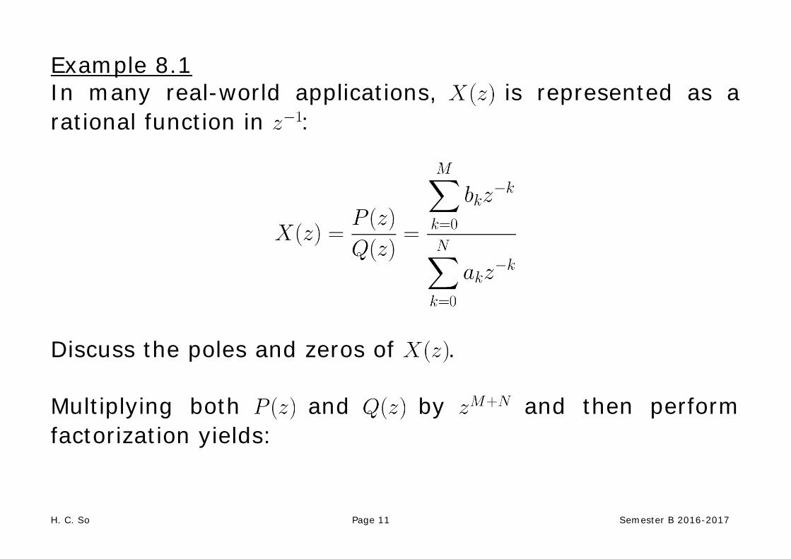
Example 8.1 In many real-world applications, is represented as a rational function in :

Discuss the poles and zeros of . Multiplying both and by and then perform factorization yields:


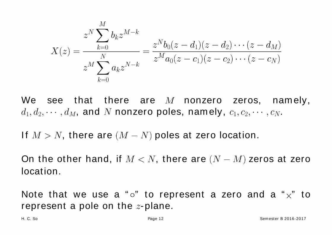
We see that there are nonzero zeros, namely,

, and nonzero poles, namely, . If , there are poles at zero location. On the other hand, if , there are zeros at zero location. Note that we use a “ ” to represent a zero and a “ ” to represent a pole on the -plane.


Example 8.2 Determine the transform of where is the unit step function. Then determine the condition when the DTFT of exists.

Using (8.1) and (2.34), we have

According to (8.7), converges if

Applying the ratio test, the convergence condition is

which aligns with the ROC for in (8.15).


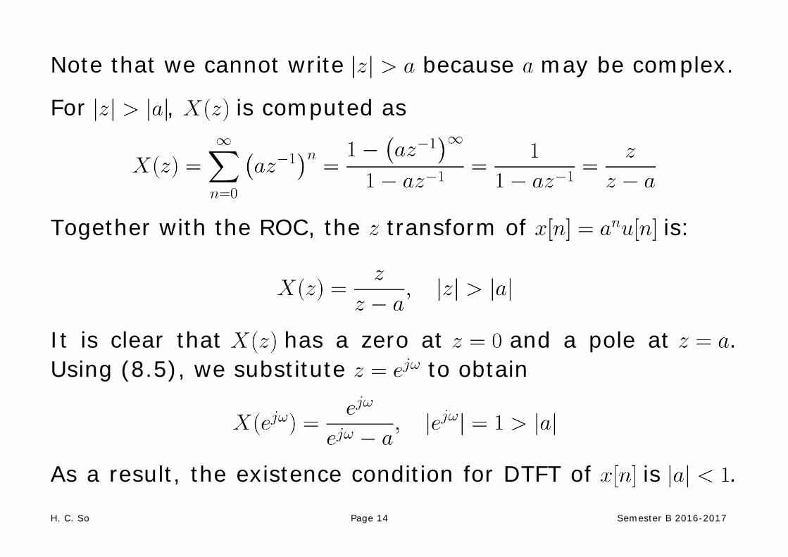
Note that we cannot write because may be complex.

For , is computed as

Together with the ROC, the transform of is:

It is clear that has a zero at and a pole at . Using (8.5), we substitute to obtain

As a result, the existence condition for DTFT of is .


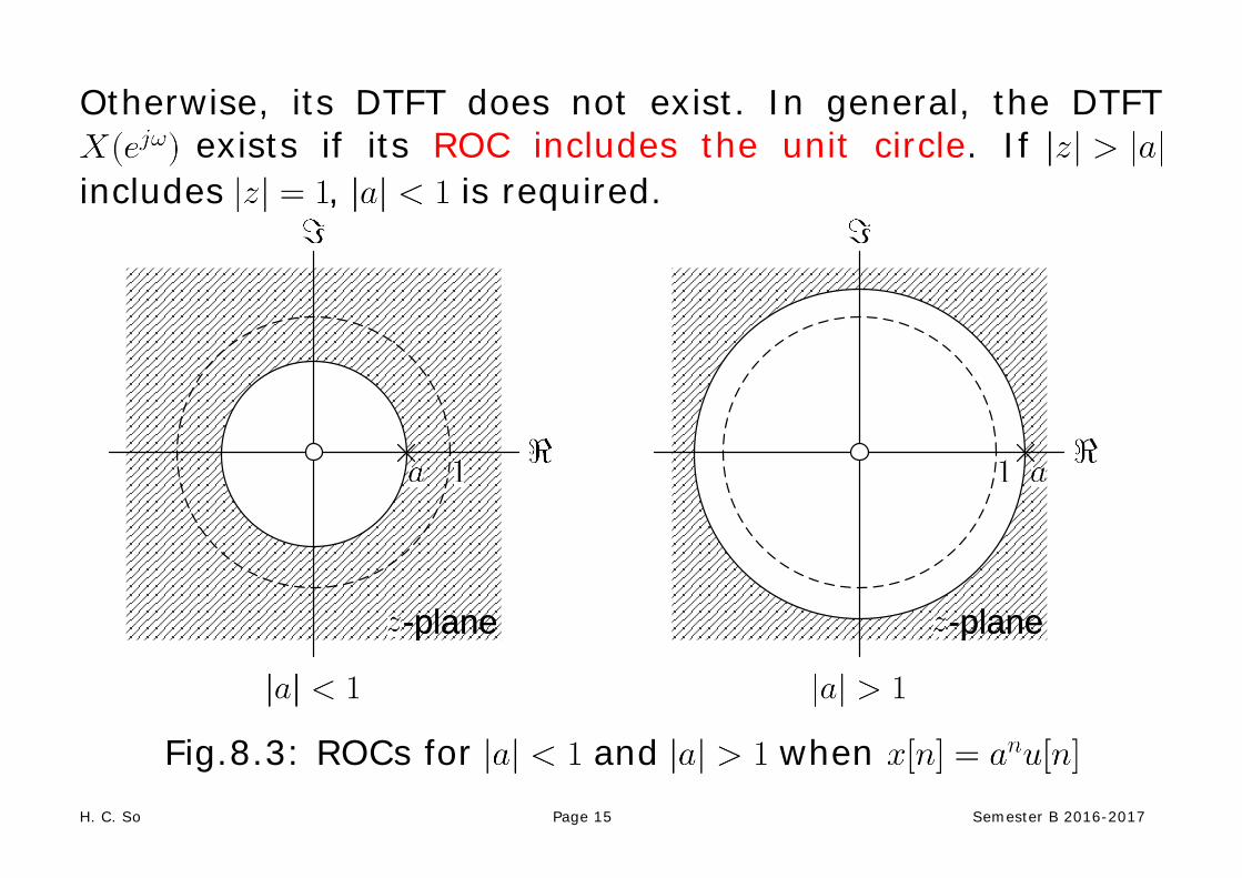
Otherwise, its DTFT does not exist. In general, the DTFT exists if its ROC includes the unit circle. If

includes , is required.

-plane -plane-plane-plane-plane-plane

Fig.8.3: ROCs for and when


Example 8.3 Determine the transform of . Then determine the condition when the DTFT of exists.


Similar to Example 8.2, converges if or , which aligns with the ROC for in (8.16). This gives

Together with ROC, the transform of is:


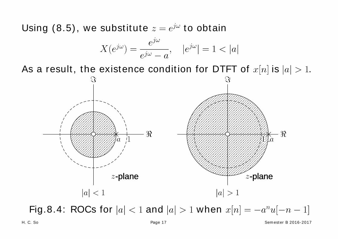
Using (8.5), we substitute to obtain

As a result, the existence condition for DTFT of is .

-plane -plane-plane-plane-plane-plane

Fig.8.4: ROCs for and when


Example 8.4 Determine the transform of where

. Employing the results in Examples 8.2 and 8.3, we have

Note that its ROC agrees with Fig. 8.2. What are the pole(s) and zero(s) of X(z)?


Example 8.5 Determine the transform of .


Example 8.6 Determine the transform of which has the form of:

Using (8.1), we have

What are the ROCs in Examples 8.5 and 8.6?


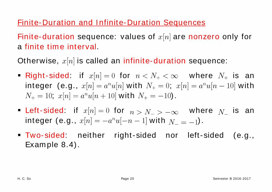
Finite-Duration and Infinite-Duration Sequences

Finite-duration sequence: values of are nonzero only for a finite time interval.

Otherwise, is called an infinite-duration sequence:

Right-sided: if for where is an integer (e.g., with ; with

; with ).

Left-sided: if for where is an integer (e.g., with ).

Two-sided: neither right-sided nor left-sided (e.g., Example 8.4).


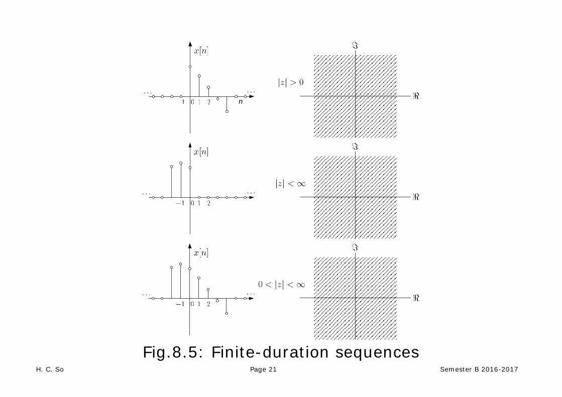
n

Fig.8.5: Finite-duration sequences


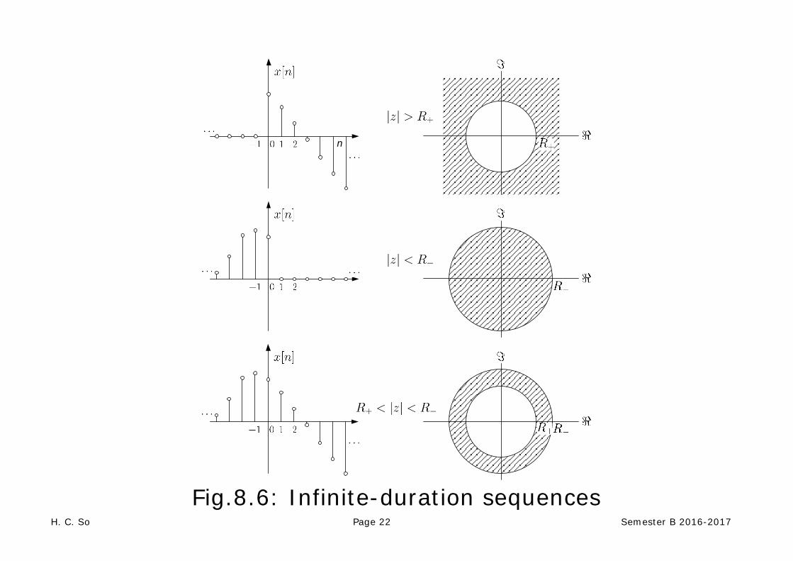
n

Fig.8.6: Infinite-duration sequences


Sequence Transform ROC 1 All

, ; ,

Table 8.1: transforms for common sequences


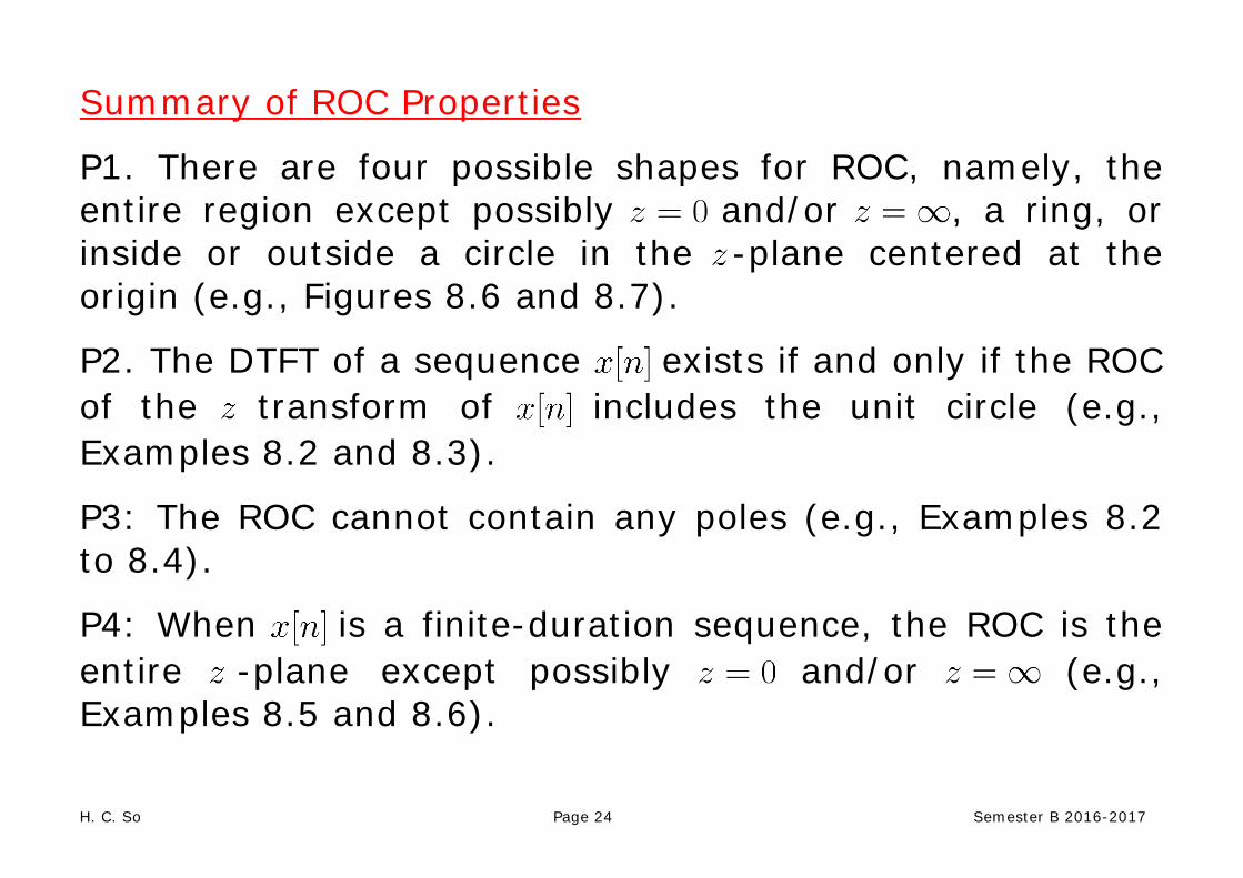
Summary of ROC Properties

P1. There are four possible shapes for ROC, namely, the entire region except possibly and/or , a ring, or inside or outside a circle in the -plane centered at the origin (e.g., Figures 8.6 and 8.7).

P2. The DTFT of a sequence exists if and only if the ROC of the transform of includes the unit circle (e.g., Examples 8.2 and 8.3).

P3: The ROC cannot contain any poles (e.g., Examples 8.2 to 8.4).

P4: When is a finite-duration sequence, the ROC is the entire -plane except possibly and/or (e.g., Examples 8.5 and 8.6).


P5: When is a right-sided sequence, the ROC is of the form where is the pole with the largest magnitude in (e.g., Example 8.2).

P6: When is a left-sided sequence, the ROC is of the form where is the pole with the smallest magnitude in (e.g., Example 8.3).

P7: When is a two-sided sequence, the ROC is of the form where and are two poles with the successive magnitudes in such that (e.g., Example 8.4).

P8: The ROC must be a connected region.

Example 8.7 A transform contains three poles, namely, , and with . Determine all possible ROCs.


-plane-plane-plane

-plane-plane-plane -plane-plane-plane

-plane-plane-plane

Fig.8.7: ROC possibilities for three poles

What are other possible ROCs?


Properties of z Transform

Linearity

Let and be two transform pairs with ROCs and , respectively, we have

(8.17)

Its ROC is denoted by , which includes where is the intersection operator. That is, contains at least the intersection of and .

Example 8.8 Determine the transform of which is expressed as:

where and .


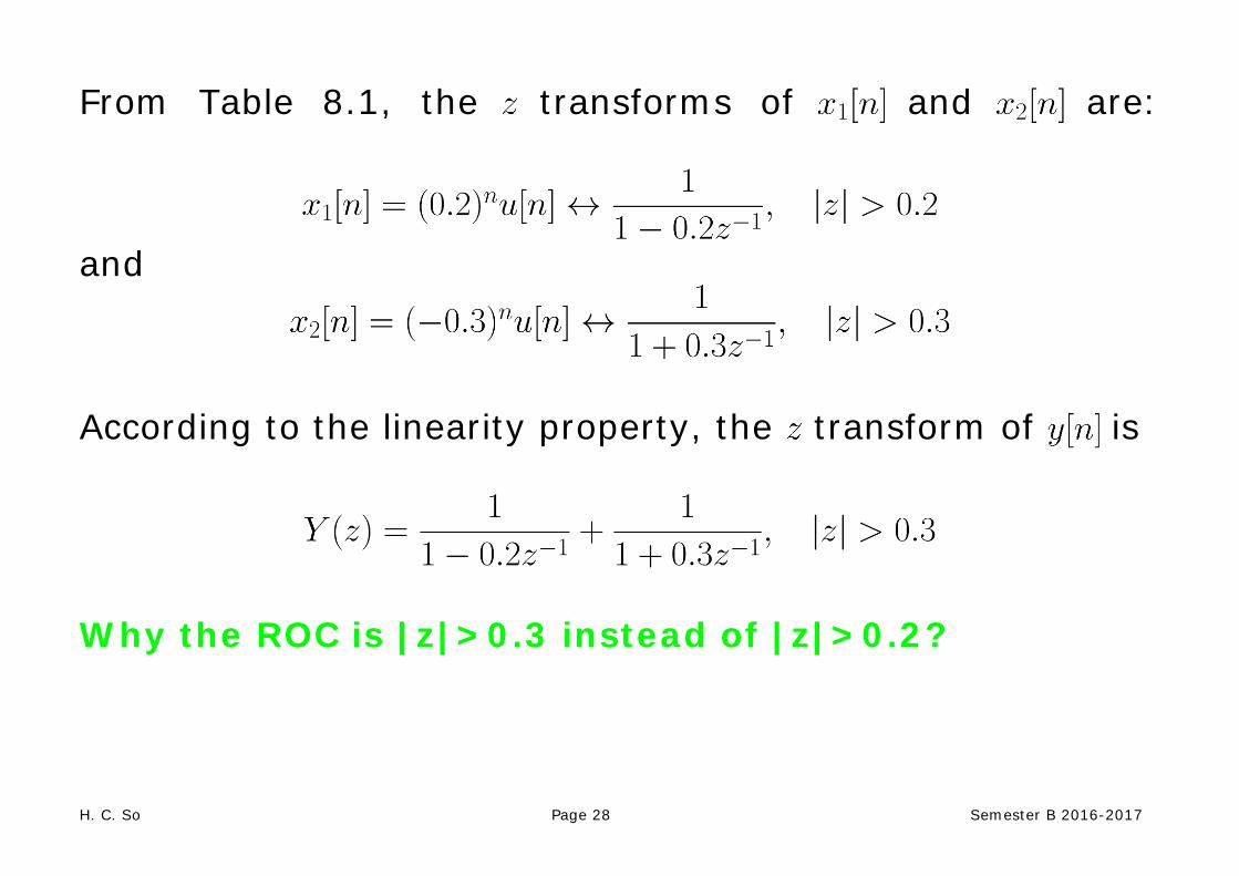
From Table 8.1, the transforms of and are:

and

According to the linearity property, the transform of is

Why the ROC is |z|>0.3 instead of |z|>0.2?


Example 8.9 Determine the ROC of the transform of which is expressed as:

Noting that , we know that the ROC of is the entire -plane.

On the other hand, both ROCs of and are . We see that the ROC of contains the

intersections of and , which is .

Time Shifting

A time-shift of in causes a multiplication of in

(8.18)

The ROC for is basically identical to that of except for the possible addition or deletion of or .


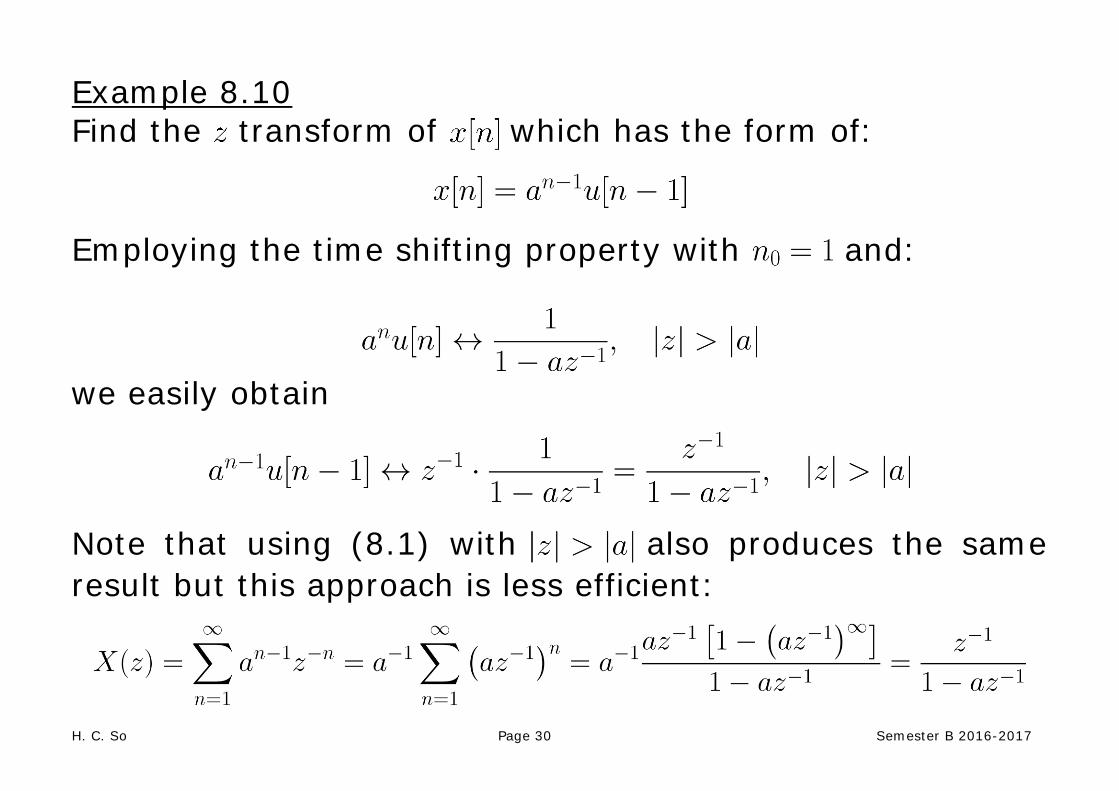
Example 8.10 Find the transform of which has the form of:

Employing the time shifting property with and:

we easily obtain

Note that using (8.1) with also produces the same result but this approach is less efficient:


Multiplication by an Exponential Sequence

If we multiply by in the time domain, the variable will be changed to in the transform domain. That is:

(8.19)

If the ROC for is , then the ROC for is .

Example 8.11 With the use of the following transform pair:

Find the transform of which has the form of:


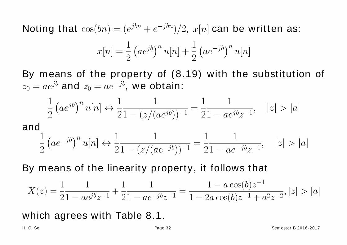
Noting that , can be written as:

By means of the property of (8.19) with the substitution of and , we obtain:

and

By means of the linearity property, it follows that

which agrees with Table 8.1.


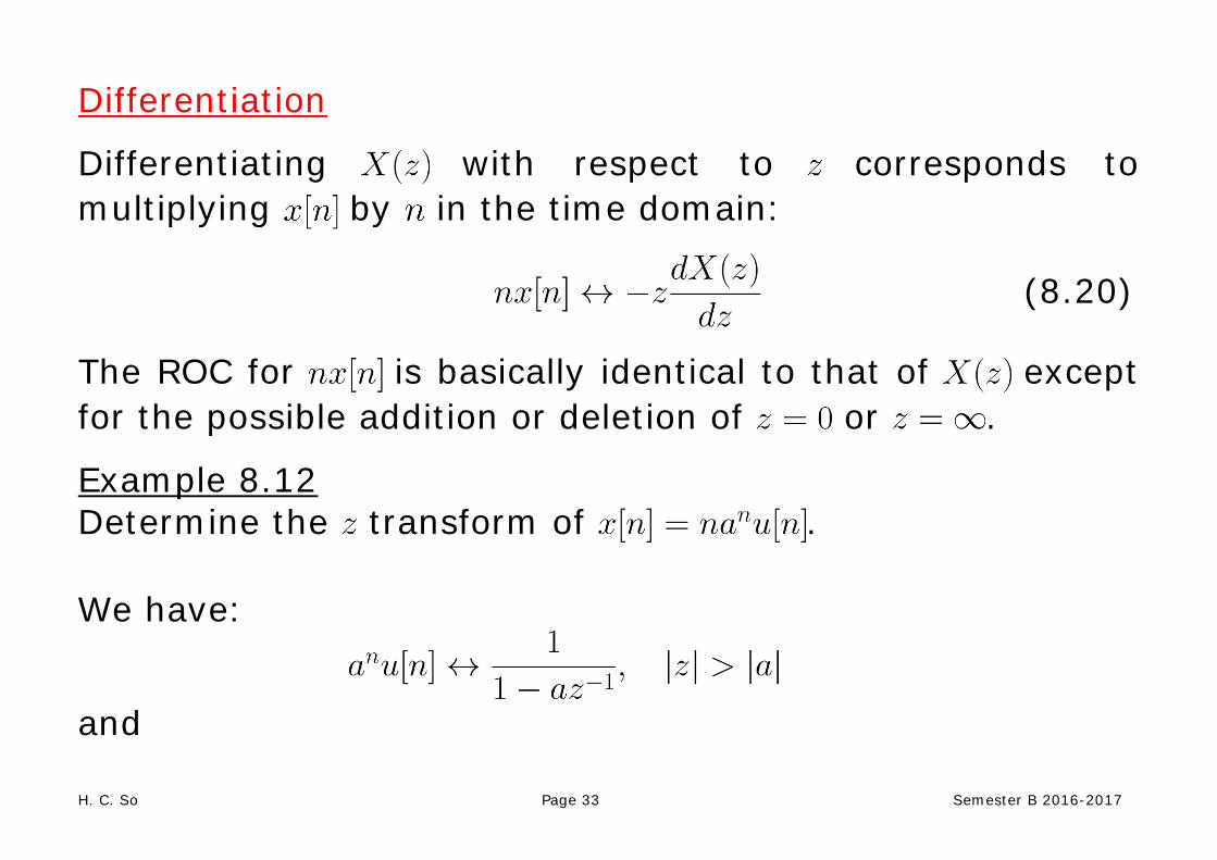
Differentiation

Differentiating with respect to corresponds to multiplying by in the time domain:

(8.20)

The ROC for is basically identical to that of except for the possible addition or deletion of or .

Example 8.12 Determine the transform of . We have:

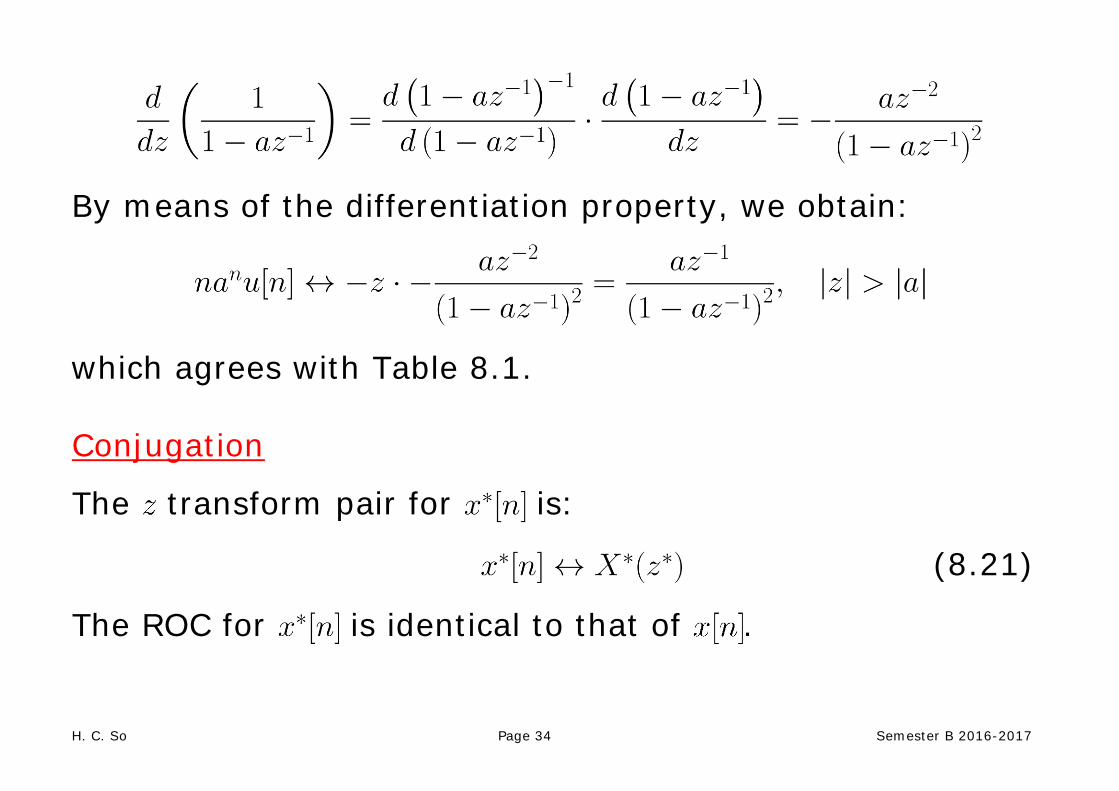
and


By means of the differentiation property, we obtain:

which agrees with Table 8.1. Conjugation

The transform pair for is:

(8.21)

The ROC for is identical to that of .


Time Reversal

The transform pair for is:

(8.22)

If the ROC for is , the ROC for is .

Example 8.13 Determine the transform of .

Using Example 8.12:

and from the time reversal property:


Convolution

Let and be two transform pairs with ROCs and , respectively. Then we have:

(8.23)

and its ROC includes .

The proof is given as follows.

Let

(8.24)


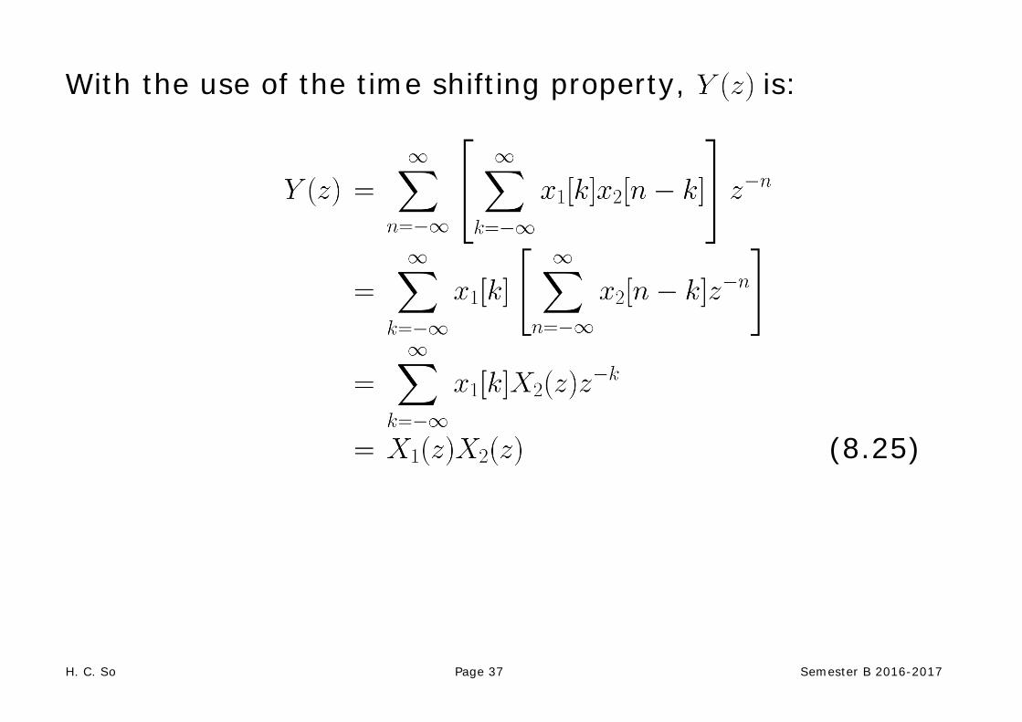
With the use of the time shifting property, is:

(8.25)


Causality and Stability Investigation with ROC Suppose is the impulse response of a discrete-time linear time-invariant (LTI) system. Recall (3.19), which is the causality condition: (8.26) If the system is causal and is of finite duration, the ROC should include (See Example 8.5 and Figure 8.5). If the system is causal and is of infinite duration, the ROC is of the form and should include (See Example 8.2 and Figure 8.6). According to P5, must be a right-sided sequence.


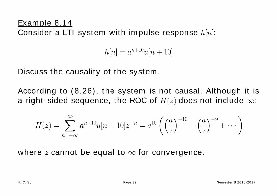
Example 8.14 Consider a LTI system with impulse response :

Discuss the causality of the system. According to (8.26), the system is not causal. Although it is a right-sided sequence, the ROC of does not include :

where cannot be equal to for convergence.


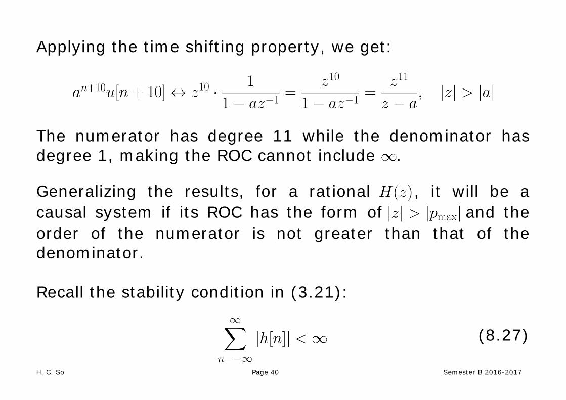
Applying the time shifting property, we get:

The numerator has degree 11 while the denominator has degree 1, making the ROC cannot include . Generalizing the results, for a rational , it will be a causal system if its ROC has the form of and the order of the numerator is not greater than that of the denominator. Recall the stability condition in (3.21):

(8.27)


Based on (8.9), this also means that the DTFT of exists.

According to P2, (8.27) indicates that the ROC of should include the unit circle. Example 8.15 Consider a LTI system with impulse response :

Discuss the stability of the system. Using the result in Example 8.14, we have:

That is, if , then the system is stable. Otherwise, the system is not stable.


Inverse z Transform

Inverse transform corresponds to finding given and its ROC.

The transform and inverse transform are one-to-one mapping provided that the ROC is given:

(8.28)

There are 4 commonly used techniques to evaluate the inverse transform. They are

1. Inspection

2. Partial Fraction Expansion

3. Power Series Expansion

4. Cauchy Integral Theorem


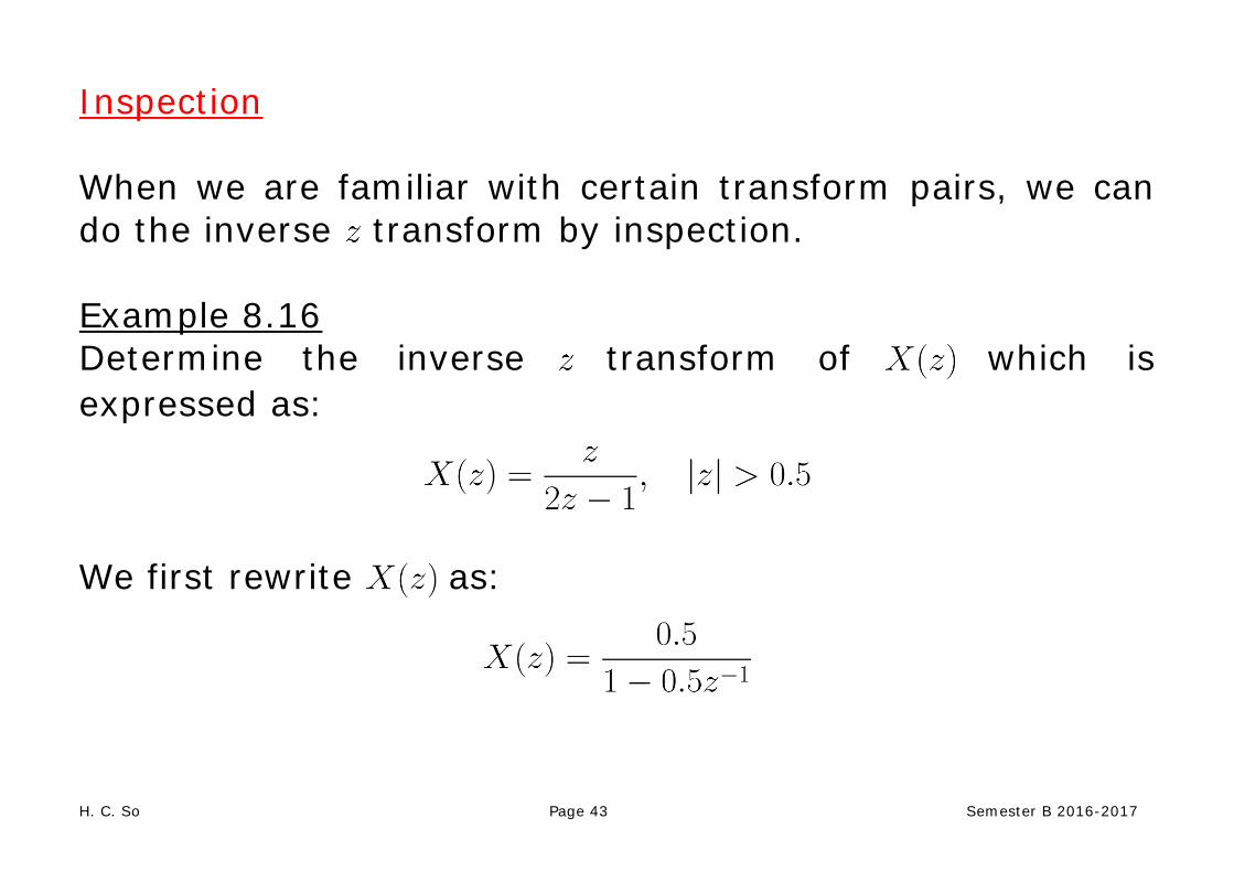
Inspection When we are familiar with certain transform pairs, we can do the inverse transform by inspection. Example 8.16 Determine the inverse transform of which is expressed as:

We first rewrite as:


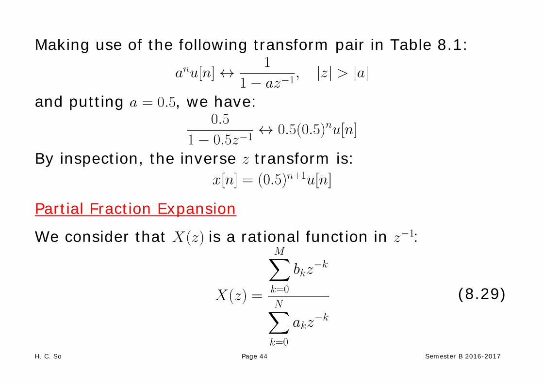
Making use of the following transform pair in Table 8.1:

and putting , we have:

By inspection, the inverse transform is:

Partial Fraction Expansion

We consider that is a rational function in :

(8.29)


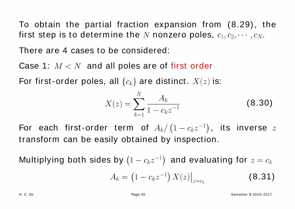
To obtain the partial fraction expansion from (8.29), the first step is to determine the nonzero poles, .

There are 4 cases to be considered:

Case 1: and all poles are of first order

For first-order poles, all are distinct. is:

(8.30)

For each first-order term of , its inverse transform can be easily obtained by inspection. Multiplying both sides by and evaluating for

(8.31)


An illustration for computing with is:

(8.32)

Substituting , we get . In summary, three steps are:

Find poles.

Find .

Perform inverse transform for the fractions by inspection.


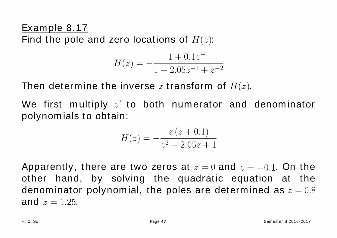
Example 8.17 Find the pole and zero locations of :

Then determine the inverse transform of .

We first multiply to both numerator and denominator polynomials to obtain:

Apparently, there are two zeros at and . On the other hand, by solving the quadratic equation at the denominator polynomial, the poles are determined as and .


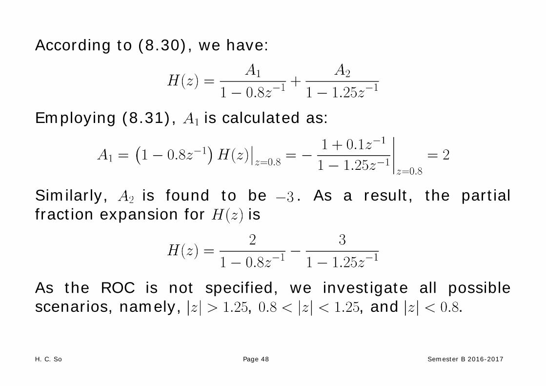
According to (8.30), we have:

Employing (8.31), is calculated as:

Similarly, is found to be . As a result, the partial fraction expansion for is

As the ROC is not specified, we investigate all possible scenarios, namely, , , and .


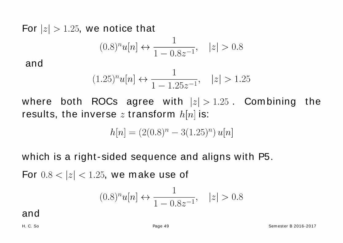
For , we notice that

and

where both ROCs agree with . Combining the results, the inverse transform is:

which is a right-sided sequence and aligns with P5.

For , we make use of

and


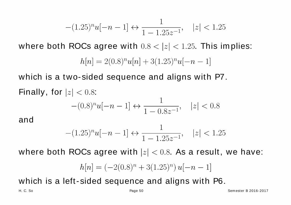
where both ROCs agree with . This implies:

which is a two-sided sequence and aligns with P7.

Finally, for :

and

where both ROCs agree with . As a result, we have:

which is a left-sided sequence and aligns with P6.


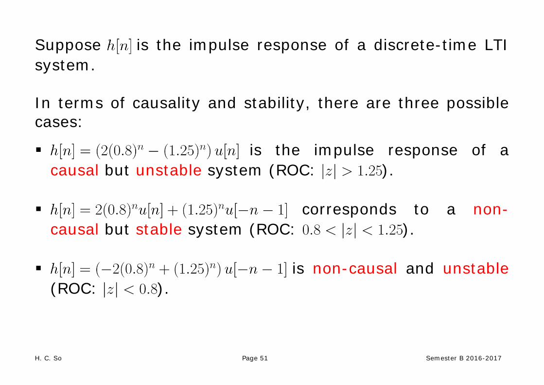
Suppose is the impulse response of a discrete-time LTI system. In terms of causality and stability, there are three possible cases:

is the impulse response of a causal but unstable system (ROC: ).

corresponds to a non-causal but stable system (ROC: ).

is non-causal and unstable

(ROC: ).


Case 2: and all poles are of first order

In this case, can be expressed as:

(8.33)

are obtained by long division of the numerator by the denominator, with the division process terminating when the remainder is of lower degree than the denominator.

can be obtained using (8.31).

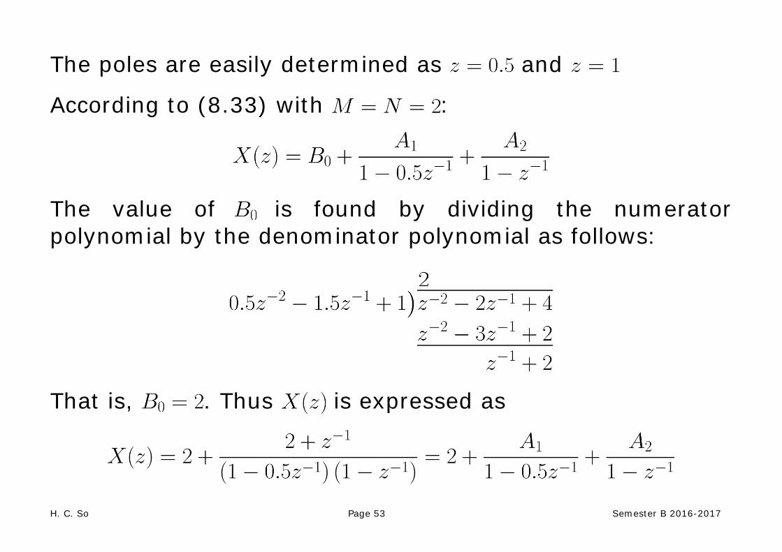
Example 8.18 Determine which has transform of the form:


The poles are easily determined as and

According to (8.33) with :

The value of is found by dividing the numerator polynomial by the denominator polynomial as follows:

That is, . Thus is expressed as


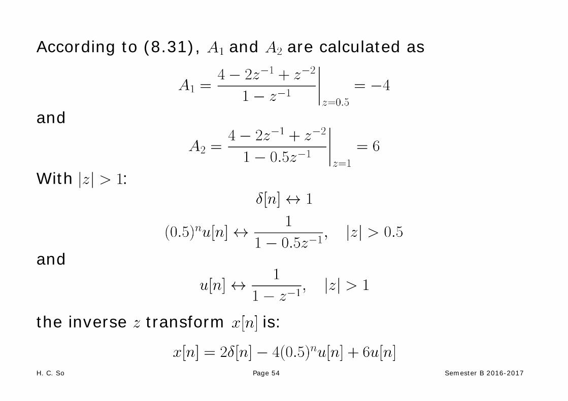
According to (8.31), and are calculated as

and

With :

and

the inverse transform is:


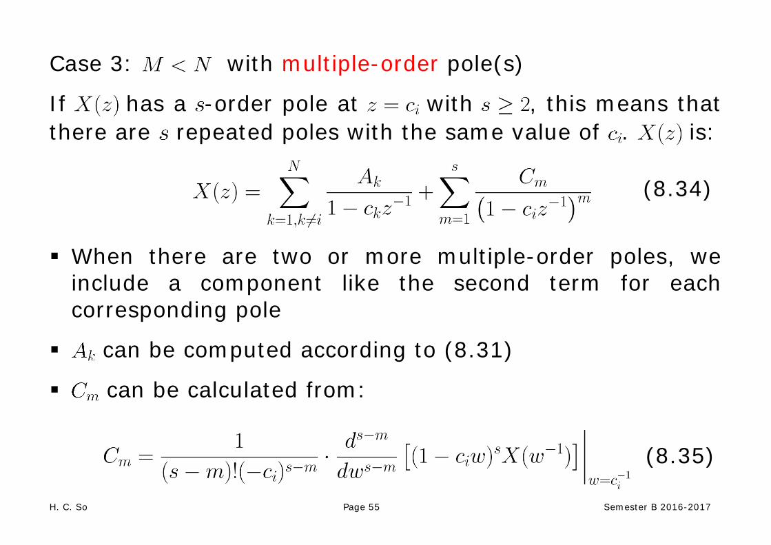
Case 3: with multiple-order pole(s)

If has a -order pole at with , this means that there are repeated poles with the same value of . is:

(8.34)

When there are two or more multiple-order poles, we include a component like the second term for each corresponding pole

can be computed according to (8.31)

can be calculated from:

(8.35)


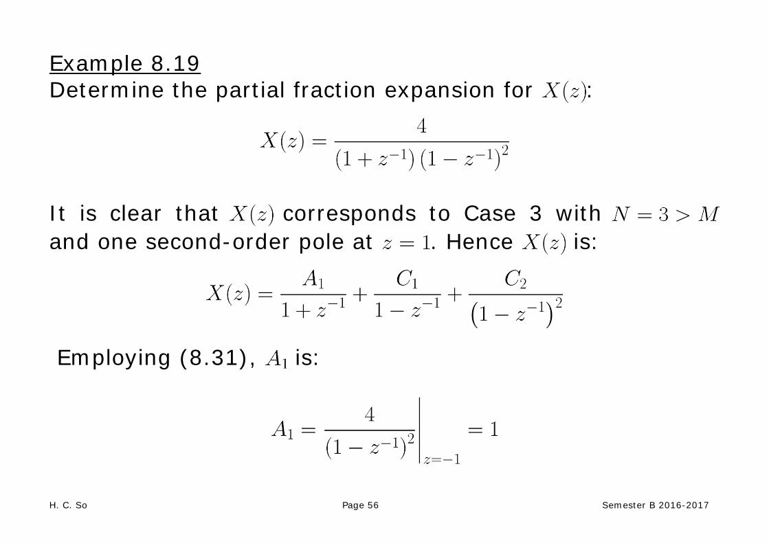
Example 8.19 Determine the partial fraction expansion for :

It is clear that corresponds to Case 3 with and one second-order pole at . Hence is:

Employing (8.31), is:


Applying (8.35), is:

and


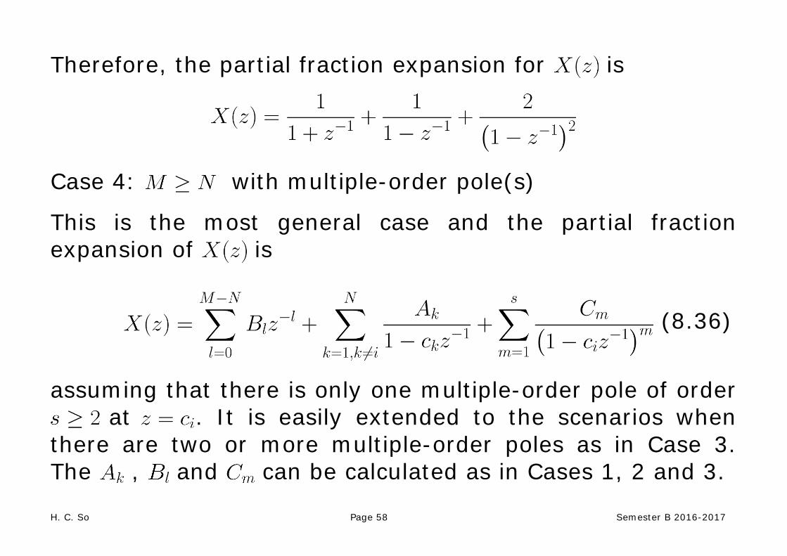
Therefore, the partial fraction expansion for is

Case 4: with multiple-order pole(s)

This is the most general case and the partial fraction expansion of is

(8.36)

assuming that there is only one multiple-order pole of order at . It is easily extended to the scenarios when

there are two or more multiple-order poles as in Case 3. The , and can be calculated as in Cases 1, 2 and 3.


Power Series Expansion

When is expanded as power series according to (5.1):

(8.37)

any particular value of can be determined by finding the coefficient of the appropriate power of

Example 8.20 Determine which has transform of the form:

Expanding yields

From (8.37), is deduced as:


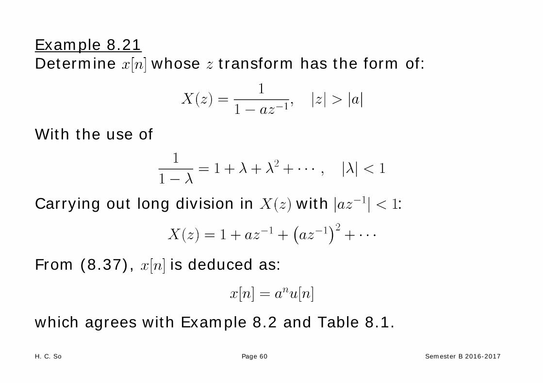
Example 8.21 Determine whose transform has the form of:

With the use of

Carrying out long division in with :


which agrees with Example 8.2 and Table 8.1.


Example 8.22 Determine whose transform has the form of:

We first express as:

Carrying out long division in with :


which agrees with Example 8.3 and Table 8.1.


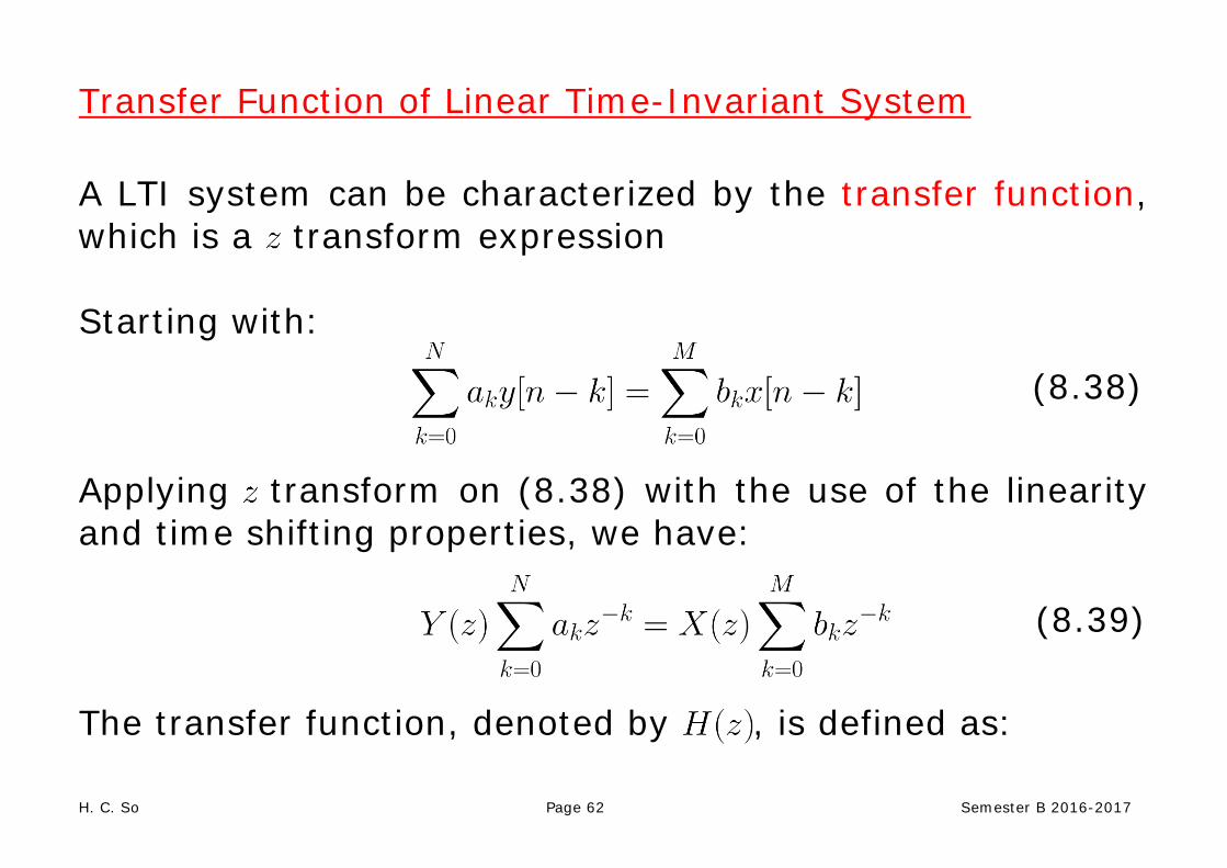
Transfer Function of Linear Time-Invariant System A LTI system can be characterized by the transfer function, which is a transform expression Starting with:

(8.38)

Applying transform on (8.38) with the use of the linearity and time shifting properties, we have:

(8.39)

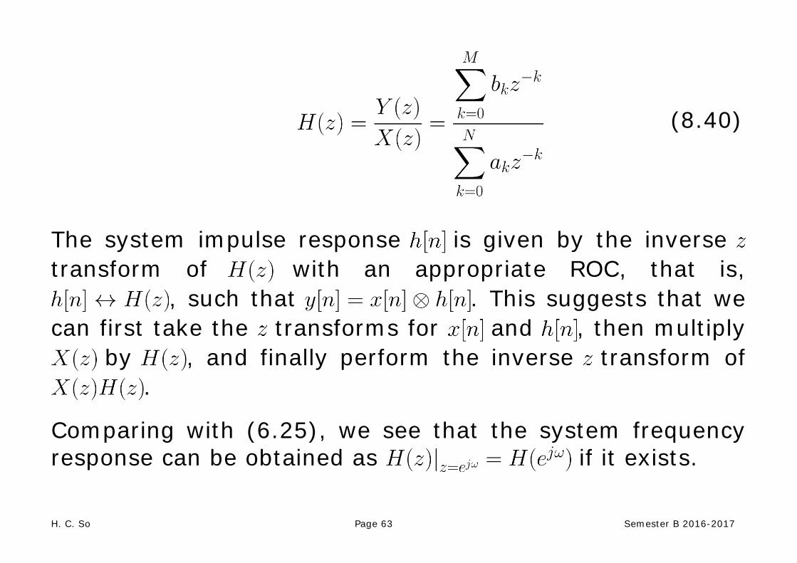
The transfer function, denoted by , is defined as:


(8.40)

The system impulse response is given by the inverse transform of with an appropriate ROC, that is,

, such that . This suggests that we can first take the transforms for and , then multiply

by , and finally perform the inverse transform of .

Comparing with (6.25), we see that the system frequency response can be obtained as if it exists.


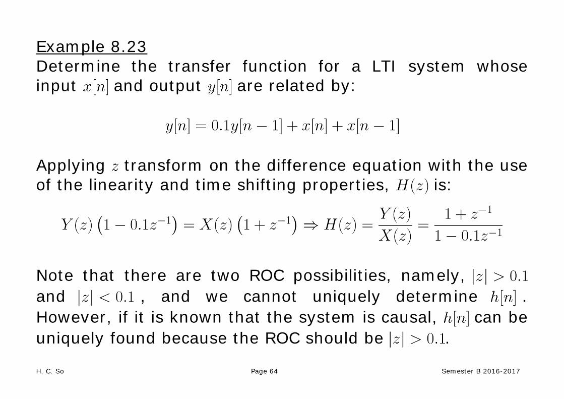
Example 8.23 Determine the transfer function for a LTI system whose input and output are related by:

Applying transform on the difference equation with the use of the linearity and time shifting properties, is:

Note that there are two ROC possibilities, namely, and , and we cannot uniquely determine . However, if it is known that the system is causal, can be uniquely found because the ROC should be .


Example 8.24 Find the difference equation of a LTI system whose transfer function is given by

Let . Performing cross-multiplication and inverse transform, we obtain:

Examples 8.23 and 8.24 imply the equivalence between the difference equation and transfer function.


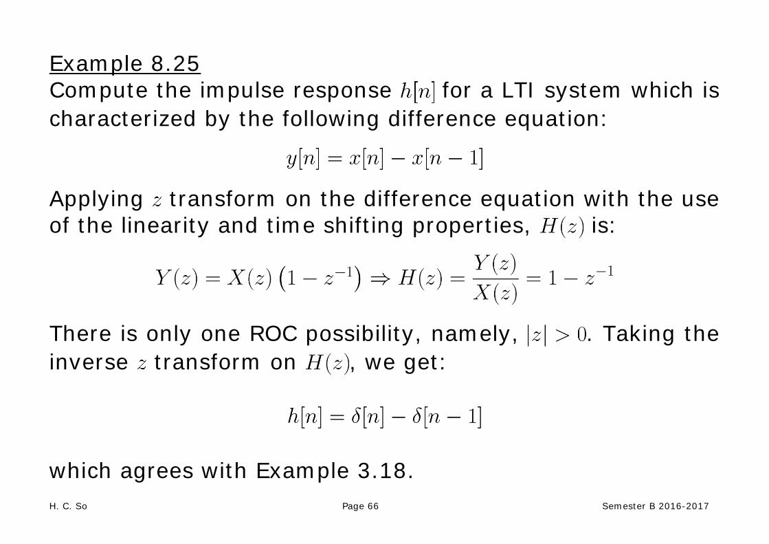
Example 8.25 Compute the impulse response for a LTI system which is characterized by the following difference equation:

Applying transform on the difference equation with the use of the linearity and time shifting properties, is:

There is only one ROC possibility, namely, . Taking the inverse transform on , we get:

which agrees with Example 3.18.


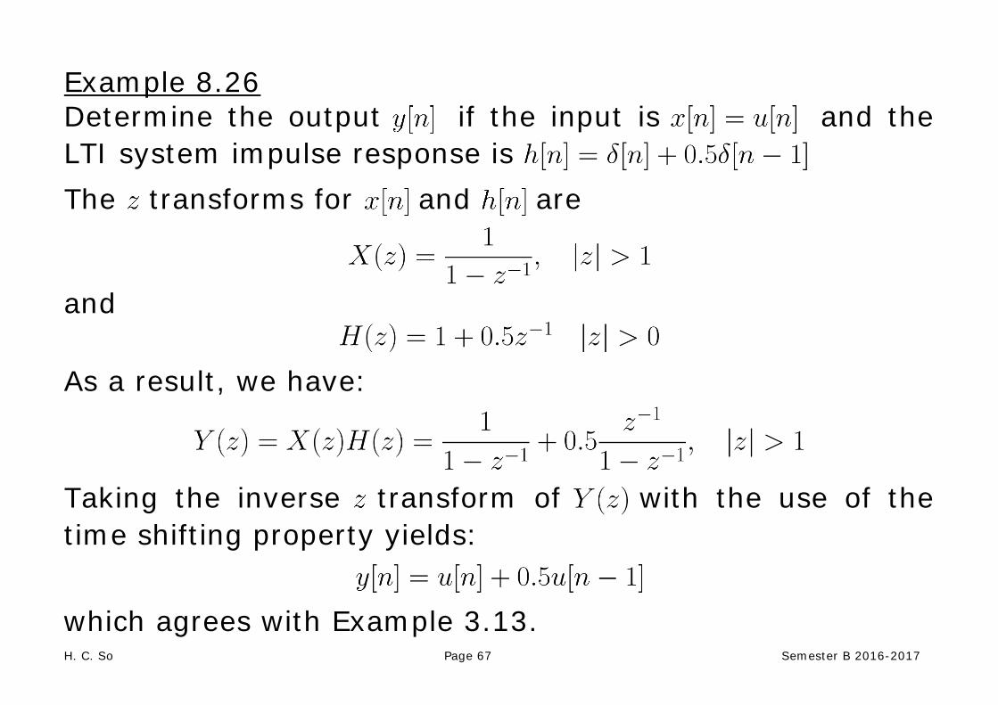
Example 8.26 Determine the output if the input is and the LTI system impulse response is

The transforms for and are

and

As a result, we have:

Taking the inverse transform of with the use of the time shifting property yields:

which agrees with Example 3.13.

z transform - department of eehcso/ee3210_8.pdfz transform. chapter intended learning outcomes: (i)...

Documents