1

Novel Folded-PCA for Improved Feature Extraction and

Data Reduction with Hyperspectral Imaging and SAR in

Remote Sensing

Jaime Zabalza1, Jinchang Ren

1, Mingqiang Yang

2, Yi Zhang

3, Jun Wang

4, Stephen Marshall

1, Junwei Han

5

1 Centre for excellence in Signal and Image Processing, Department of Electronic and Electrical Engineering,

University of Strathclyde, Glasgow, United Kingdom 2 School of Information Science and Technology, Shandong University, Jinan, China

3 School of Computer Software, Tianjin University, Tianjin, China

4 School of Electronic and Information Engineering, Beijing Univ. of Aeronautics and Astronautics, China

5 School of Automation, Northwestern Polytechnical University, Xi’an, China

j.zabalza@strah.ac.uk jinchang.ren@strath.ac.uk yangmq@sdu.edu.cn yizhang@tju.edu.cn

wangj203@buaa.edu.cn Stephen.Marshall@strath.ac.uk jhan@nwpu.edu.cn

Abstract—As a widely used approach for feature extraction and data reduction, Principal Components Analysis (PCA) suffers from

high computational cost, large memory requirement and low efficacy in dealing with large dimensional datasets such as Hyperspectral

Imaging (HSI). To this end, a novel Folded-PCA is proposed, in which the spectral vector is folded into a matrix to allow the covariance

matrix to be determined in a more efficient way. With this matrix-based representation, both global and local structures can be extracted

to provide additional information for data classification. In addition, both the computational cost and the memory requirement have been

significantly reduced. Using Support Vector Machine (SVM) for classification on two well-known HSI datasets and one Synthetic

Aperture Radar (SAR) dataset in remote sensing applications, quantitative results are generated for objective evaluations.

Comprehensive results have indicated that the proposed Folded-PCA approach not only outperforms the conventional PCA but also the

baseline approach where the whole feature sets are used.

Keywords—Folded Principal Component Analysis (F-PCA), feature extraction, data reduction, Hyperspectral Imaging (HSI), Support

Vector Machine (SVM), remote sensing.

Corresponding Author:

Dr Jinchang Ren

Hyperspectral Imaging Centre,

Dept. of Electronic and Electrical Engineering

University of Strathclyde

Glasgow, G1 1XW

United Kingdom Email: jinchang.ren@strath.ac.uk Tel. +44-141-5482384

2

I. INTRODUCTION

Through capturing data from numerous and contiguous spectral bands, Hyperspectral Imaging (HSI) has provided a unique and

invaluable solution for a number of application areas. With the large spectral range covered from visible light to (near) infrared, HSI

is capable of detecting and identifying the minute differences of objects and their changes in temperature and moisture. As a result,

the applications of HSI have been extended from traditional ones such as remote sensing, mining, agriculture, geology and military

surveillance to many newly emerging lab-based data analysis. These new applications include food quality, pharmaceutical, security

and skin cancer analysis as well as verification of counterfeit goods and documents [1-2].

In general, HSI data forms a hypercube, containing 2D spatial information and 1D spectral information. Consequently, the total

data contained is XYF, where each of the symbols denotes the spatial height, spatial width and the number of spectral bands of the

hypercube, respectively. With a spectral resolution in nanometers, HSI enables high discrimination ability in data analysis, at the

cost of extremely large datasets and computational complexity.

When the ratio between the number of features (spectral bands) and the number of training samples (sample pixels) is unbalanced,

large dimensional data such as HSI suffers from the curse of dimensionality issue, also known as the Hughes effect [3]. As a result,

in the hyperspectral context, such unbalance becomes a severe problem, especially when the hypercube contains pixels of multiple

classes. Consequently, effective feature extraction and data reduction is required. Due to the high redundancy between neighboring

spectral bands, such data reduction is feasible [4].

For feature extraction and dimension reduction in hypercubes, the most widely used approach is Principal Components Analysis

(PCA) [5], followed by several other approaches such as random projection [6], singular value decomposition [7] and maximum

noise fraction [8]. In fact, PCA uses orthogonal transformation to convert high dimensional data into linearly uncorrelated variables,

namely principal components. Often, the number of principal components is significantly reduced in comparison to the original

feature dimension, here referring to the number of bands. Consequently, PCA is found to be a powerful tool in feature extraction and

data reduction.

Let S=XY represent the spatial size of a hypercube. In conventional PCA analysis, the hypercube needs to be converted to an F×S

matrix, whose covariance matrix is then determined for principal component extraction. Basically, this process involves two

challenges. One is the difficulty in obtaining the covariance matrix when the dimension S is extremely large, usually over 100k,

which often causes software tools such as Matlab crashed due to problems of memory management. The other is that it fails to

pick-up the disparate contributions of the featured F bands as these bands are equally treated when the covariance matrix is

obtained.

To address the aforementioned two challenges, in this paper, a novel Folded-PCA (F-PCA) method is proposed. In our approach,

3

the covariance matrix is obtained by accumulation of S partial covariance matrices, which are obtained from a much smaller matrix

formed by folding the featured F bands into a matrix. As such, the correlation between bands and band groups are successfully

extracted in calculating the partial covariance matrix. To this end, improved results with reduced computational burden on data

reduction and feature extraction are achieved.

The remaining part of this paper is organised as follows. Section II summarises the principles of conventional PCA and its

variants. In Section III, the proposed Folded-PCA approach is presented. Datasets and experimental setup are discussed in Section

IV, with comprehensive results reported in Section V. Finally, some concluding marks are drawn in Section VI.

II. APPLYING CONVENTIONAL PCA IN HSI

PCA, also known as the Karhunen-Loeve Transform (KLT), is an unsupervised method for feature extraction and data reduction [9].

With a clear mathematical procedure defined for straightforward implementation, PCA has been widely used in many applications.

In general, PCA can reduce the number of features by removing the correlation among the data, and this is achieved by orthogonal

projection and truncation of the transformed feature data. Consequently, data samples can be represented in a lower dimensional

space for fast but more effective analysis, such as improved coding [10] and classification [11-12].

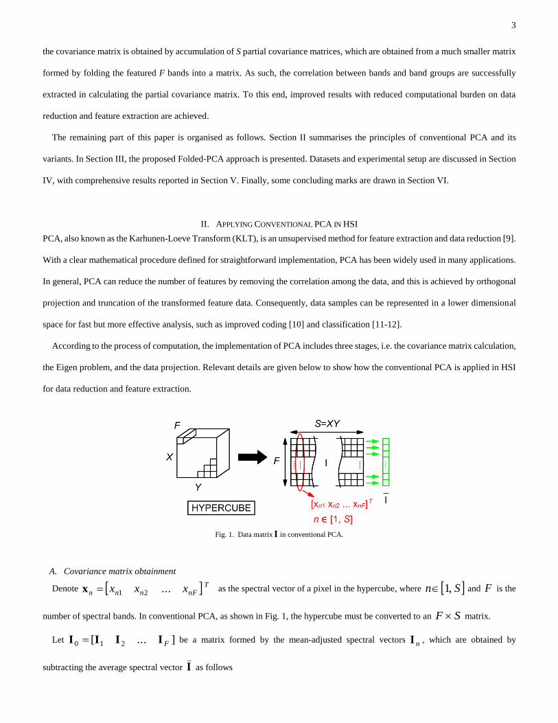
According to the process of computation, the implementation of PCA includes three stages, i.e. the covariance matrix calculation,

the Eigen problem, and the data projection. Relevant details are given below to show how the conventional PCA is applied in HSI

for data reduction and feature extraction.

Fig. 1. Data matrix I in conventional PCA.

A. Covariance matrix obtainment

Denote TnFnnn xxx ...21x as the spectral vector of a pixel in the hypercube, where Sn ,1 and F is the

number of spectral bands. In conventional PCA, as shown in Fig. 1, the hypercube must be converted to an SF matrix.

Let ]...[ 210 FIIII be a matrix formed by the mean-adjusted spectral vectors nI , which are obtained by

subtracting the average spectral vector I as follows

4

S

n n

nn

S 1

1xI

IxI

(1)

Therefore, nI becomes a mean-adjusted vector. For the matrix

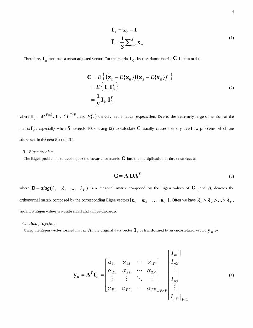
0I , its covariance matrix C is obtained as

T

Tnn

T

nnnn

S

E

EEE

00

1

}{}{

II

II

xxxxC

(2)

where SF0I ,

FFC , and {.}E denotes mathematical expectation. Due to the extremely large dimension of the

matrix0I , especially when S exceeds 100k, using (2) to calculate C usually causes memory overflow problems which are

addressed in the next Section III.

B. Eigen problem

The Eigen problem is to decompose the covariance matrix C into the multiplication of three matrices as

TDΛΛC (3)

where )...( 21 Fdiag D is a diagonal matrix composed by the Eigen values of C , and Λ denotes the

orthonormal matrix composed by the corresponding Eigen vectors ]...[ 21 Fααα . Often we have F ...21

,

and most Eigen values are quite small and can be discarded.

C. Data projection

Using the Eigen vector formed matrix Λ , the original data vector nI is transformed to an uncorrelated vector

ny by

1

2

1

21

22221

11211

FnF

nq

n

n

FFFFFF

F

F

nT

n

I

I

I

I

IΛy (4)

5

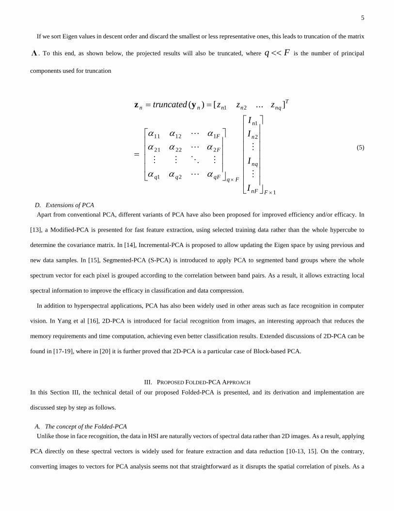
If we sort Eigen values in descent order and discard the smallest or less representative ones, this leads to truncation of the matrix

Λ . To this end, as shown below, the projected results will also be truncated, where Fq is the number of principal

components used for truncation

1

2

1

21

22221

11211

21 ]...[)(

FnF

nq

n

n

FqqFqq

F

F

Tnqnnnn

I

I

I

I

zzztruncated

yz

(5)

D. Extensions of PCA

Apart from conventional PCA, different variants of PCA have also been proposed for improved efficiency and/or efficacy. In

[13], a Modified-PCA is presented for fast feature extraction, using selected training data rather than the whole hypercube to

determine the covariance matrix. In [14], Incremental-PCA is proposed to allow updating the Eigen space by using previous and

new data samples. In [15], Segmented-PCA (S-PCA) is introduced to apply PCA to segmented band groups where the whole

spectrum vector for each pixel is grouped according to the correlation between band pairs. As a result, it allows extracting local

spectral information to improve the efficacy in classification and data compression.

In addition to hyperspectral applications, PCA has also been widely used in other areas such as face recognition in computer

vision. In Yang et al [16], 2D-PCA is introduced for facial recognition from images, an interesting approach that reduces the

memory requirements and time computation, achieving even better classification results. Extended discussions of 2D-PCA can be

found in [17-19], where in [20] it is further proved that 2D-PCA is a particular case of Block-based PCA.

III. PROPOSED FOLDED-PCA APPROACH

In this Section III, the technical detail of our proposed Folded-PCA is presented, and its derivation and implementation are

discussed step by step as follows.

A. The concept of the Folded-PCA

Unlike those in face recognition, the data in HSI are naturally vectors of spectral data rather than 2D images. As a result, applying

PCA directly on these spectral vectors is widely used for feature extraction and data reduction [10-13, 15]. On the contrary,

converting images to vectors for PCA analysis seems not that straightforward as it disrupts the spatial correlation of pixels. As a

6

result, 2D-PCA, also namely Image-based PCA, is found to be more effective in this context [16]. This has inspired us to propose

our Folded-PCA approach below. Therefore, while conventional PCA takes vectors as input, in the proposed approach, the spectral

vector is folded into a matrix to enable 2D-PCA style analysis. The 2D folding scheme here, however, does not aim to solve the

spatial disruption but to extract local structures in the spectral domain. Though it seems similar to the Segmented-PCA [15], reduced

computational complexity is achieved as further discussed in the next Section V.

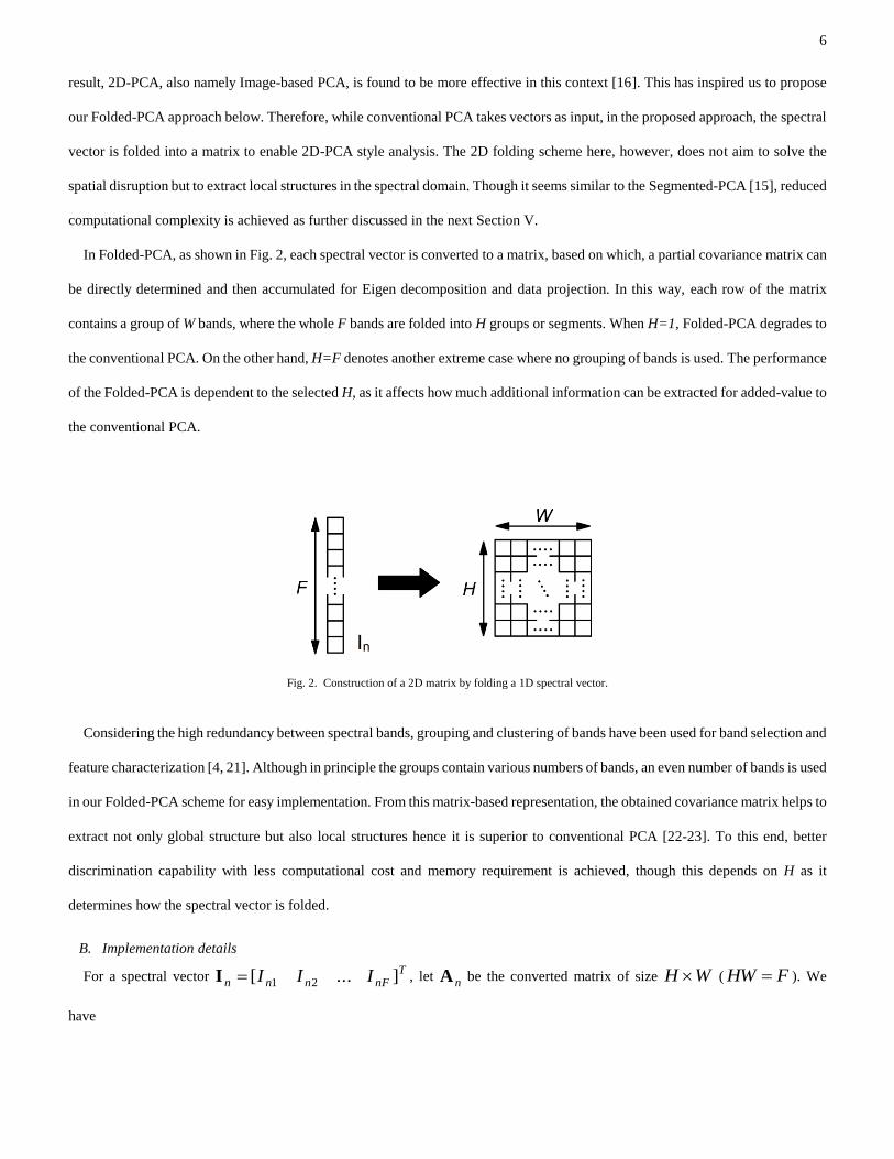
In Folded-PCA, as shown in Fig. 2, each spectral vector is converted to a matrix, based on which, a partial covariance matrix can

be directly determined and then accumulated for Eigen decomposition and data projection. In this way, each row of the matrix

contains a group of W bands, where the whole F bands are folded into H groups or segments. When H=1, Folded-PCA degrades to

the conventional PCA. On the other hand, H=F denotes another extreme case where no grouping of bands is used. The performance

of the Folded-PCA is dependent to the selected H, as it affects how much additional information can be extracted for added-value to

the conventional PCA.

Fig. 2. Construction of a 2D matrix by folding a 1D spectral vector.

Considering the high redundancy between spectral bands, grouping and clustering of bands have been used for band selection and

feature characterization [4, 21]. Although in principle the groups contain various numbers of bands, an even number of bands is used

in our Folded-PCA scheme for easy implementation. From this matrix-based representation, the obtained covariance matrix helps to

extract not only global structure but also local structures hence it is superior to conventional PCA [22-23]. To this end, better

discrimination capability with less computational cost and memory requirement is achieved, though this depends on H as it

determines how the spectral vector is folded.

B. Implementation details

For a spectral vector T

nFnnn III ]...[ 21I , let nA be the converted matrix of size WH ( FHW ). We

have

7

]...[ ))1(())1(2())1(1(

2

1

hWWnhWnhWnnh

WHnH

n

n

n

IIIa

a

a

a

A

(6)

where ],1[ Hh . The selection of different values of H (and hence W ) may affect the results, which will be demonstrated in

Section V.

For the matrix nA , its covariance matrix is obtained by

WWnn

Tnn

CAAC , (7)

Eventually, the overall covariance matrix for the whole hypercube is determined as the accumulation of these partial covariance

matrices as follows

S

n nTn

S

n nFPCASS 11

11AACC (8)

where again S represents the spatial size of the hypercube.

From FPCAC , the same methodology in (3) is applied for the Eigen decomposition. However, it is worth noting that

FPCAC is

sized of WW , whilst the covariance matrix from conventional PCA in (2) is sized of FF , or HWHW . As a result,

the computational costs for the Eigen problem in our Folded-PCA have been significantly reduced.

Regarding the data projection part, Eqs. (4), (5) for conventional PCA need to be adjusted to cope with the input in folded-vector,

i.e. the matrix WH

nA , rather than the spectral vector

nI . For the covariance matrix FPCAC , let 'q be the number of

selected Eigen values and 'qWΛ the matrix formed using Eigen vectors for data projection. For each row vector in

nA , 'q

components are extracted by multiplying it with Λ , which results in 'Hqq features extracted for the whole sample. In other

words, the data obtained from projection, 'qH

nZ , is determined by multiplying two smaller matrices as follows, which has

also significantly reduced the computational cost

',, qWWHnnn

ΛAΛAZ (9)

8

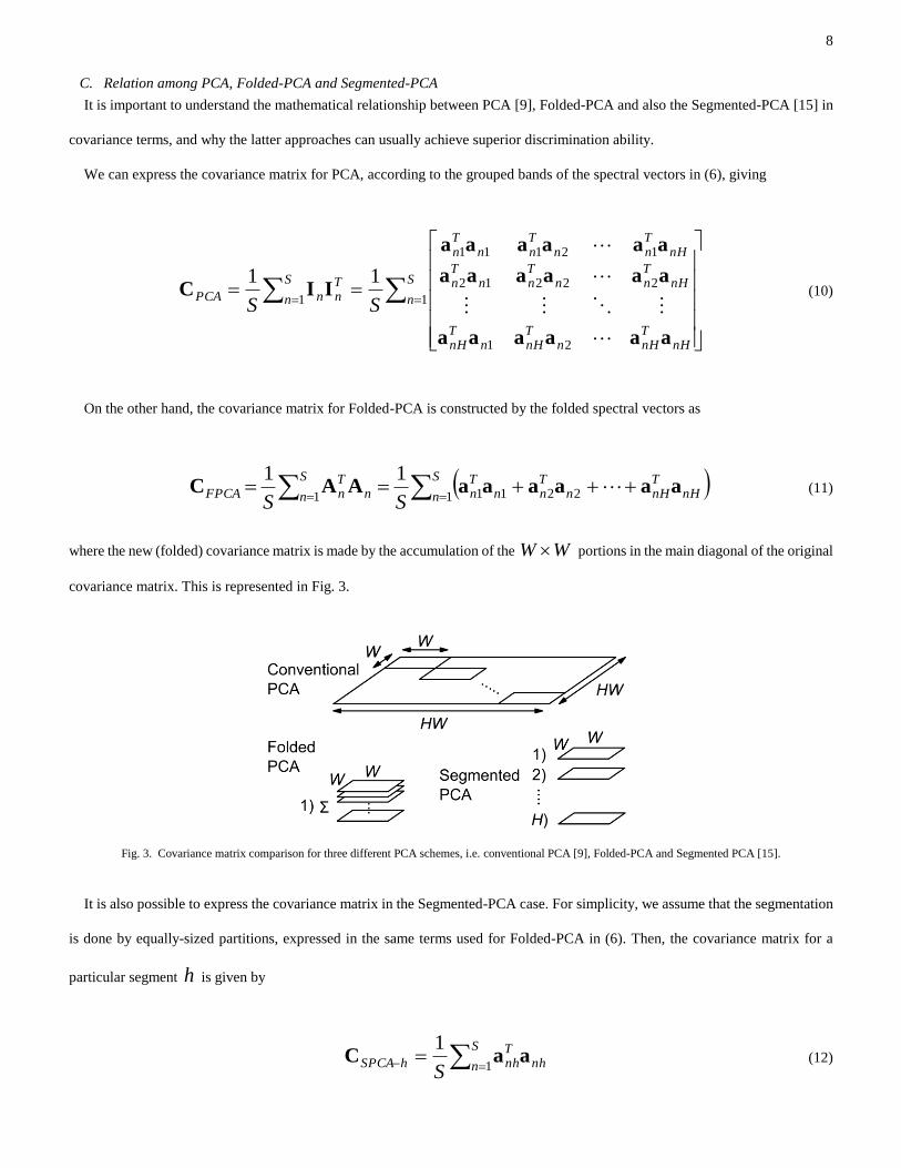
C. Relation among PCA, Folded-PCA and Segmented-PCA

It is important to understand the mathematical relationship between PCA [9], Folded-PCA and also the Segmented-PCA [15] in

covariance terms, and why the latter approaches can usually achieve superior discrimination ability.

We can express the covariance matrix for PCA, according to the grouped bands of the spectral vectors in (6), giving

S

n

nHTnHn

TnHn

TnH

nHTnn

Tnn

Tn

nHTnn

Tnn

Tn

Tn

S

n nPCASS 1

21

22212

12111

1

11

aaaaaa

aaaaaa

aaaaaa

IIC

(10)

On the other hand, the covariance matrix for Folded-PCA is constructed by the folded spectral vectors as

S

n nHTnHn

Tnn

Tn

S

n nTnFPCA

SS 1 22111

11aaaaaaAAC (11)

where the new (folded) covariance matrix is made by the accumulation of the WW portions in the main diagonal of the original

covariance matrix. This is represented in Fig. 3.

Fig. 3. Covariance matrix comparison for three different PCA schemes, i.e. conventional PCA [9], Folded-PCA and Segmented PCA [15].

It is also possible to express the covariance matrix in the Segmented-PCA case. For simplicity, we assume that the segmentation

is done by equally-sized partitions, expressed in the same terms used for Folded-PCA in (6). Then, the covariance matrix for a

particular segment h is given by

S

n nhTnhhSPCA

S 1

1aaC (12)

9

In Segmented-PCA [15], there are as many covariance matrices (and their respective PCA implementations) as segments in the

partition. This is the fundamental difference from our proposed Folded-PCA, where all the locally extracted covariance matrices are

combined together thus the Eigen problem needs to be solved just once.

The advantages of using the proposed Folded-PCA are summarized as follows. The first is improved discrimination capability as

in Folded-PCA the matrix-like analysis enables extraction of local structure [22-23] from the hypercube spectral domain. This is

achieved by extracting features from each grouped bands, i.e. the row vectors in nA , to ensure local features within these band

groups are covered. The second is significantly reduced complexity of the overall algorithm due to a much smaller covariance

matrix being required. The third is reduced memory usage in determining the covariance matrix and subsequent analysis. Relevant

experiments and novel results are reported in Section V.

An important consideration in our approach is how to select appropriate values for parameters H (or W ) and q (or 'q ). From

our point of view, similar to Segmented-PCA [15], the selection is related to the common distribution of correlation among the

spectral bands. In general, contiguous spectral bands in HSI are highly correlated, thus it is useful to group these bands into sub-sets

for efficiency. Although the strict number of bands contained in each group varies, using even number of bands in our approach has

significantly simplified the problem, where the improved performance in classification is also reported in Section V.

As observed in the Segmented-PCA [15], bands are grouped based on the correlation matrix between each pair of them. In the

Folded-PCA approach, the number of bands W is selected according to the common or averaged dimensions of the clusters that

can be observed in the main diagonal of this correlation matrix. As a result, this criterion is a general recommendation and allows

several different possible segmentations. For 'q , it is asked to be a small portion of W , usually 10-25%, as a large number of 'q

may lead to more noisy features as demonstrated in Section V.C (Figs. 7-8).

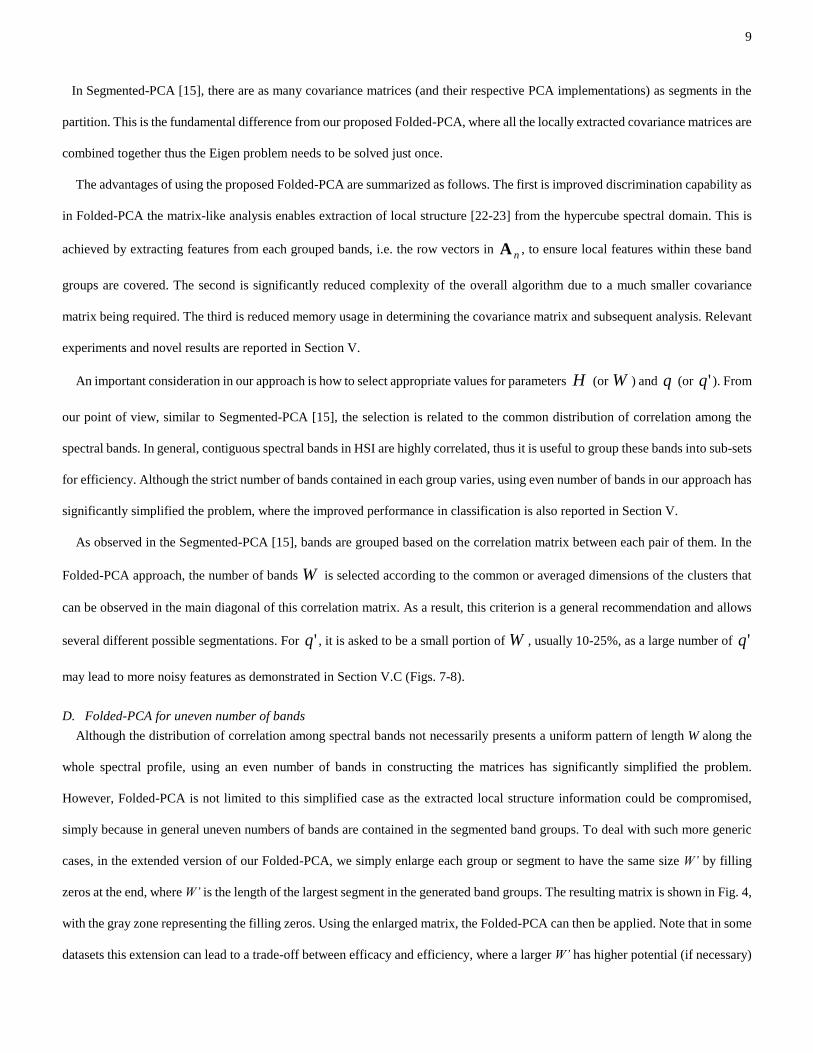
D. Folded-PCA for uneven number of bands

Although the distribution of correlation among spectral bands not necessarily presents a uniform pattern of length W along the

whole spectral profile, using an even number of bands in constructing the matrices has significantly simplified the problem.

However, Folded-PCA is not limited to this simplified case as the extracted local structure information could be compromised,

simply because in general uneven numbers of bands are contained in the segmented band groups. To deal with such more generic

cases, in the extended version of our Folded-PCA, we simply enlarge each group or segment to have the same size W’ by filling

zeros at the end, where W’ is the length of the largest segment in the generated band groups. The resulting matrix is shown in Fig. 4,

with the gray zone representing the filling zeros. Using the enlarged matrix, the Folded-PCA can then be applied. Note that in some

datasets this extension can lead to a trade-off between efficacy and efficiency, where a larger W’ has higher potential (if necessary)

10

for local structure extraction yet less reduction in computational complexity.

Fig. 4. Construction of a 2D matrix by folding a 1D spectral vector with uneven number of bands for each segment.

IV. EXPERIMENTAL SETUP

Although a hypercube is utilized to derive the Folded-PCA, the proposed approach can be applied in general applications for data

reduction and feature extraction from large dimensional datasets. To this end, in our experiments, both hyperspectral datasets and

real Synthetic Aperture Radar (SAR) data are employed to fully validate the efficiency and efficacy of our proposed methodology.

The data and experimental settings are organized in four stages, i.e. data description, data conditioning, feature extraction and

classification. These are discussed in detail below.

A. Data description

Three datasets with available ground truth are employed in our experiments for evaluation, which include two datasets of remote

sensing in HSI and a group of real SAR data of micro-Doppler radar signatures. The remote sensing datasets are sub-scenes

extracted from the original North-South Flightline hypercube, collected by the AVIRIS instrument over an agricultural study site in

Northwest Indiana [24-25], which has been widely used in applications for feature selection and classification [26-30].

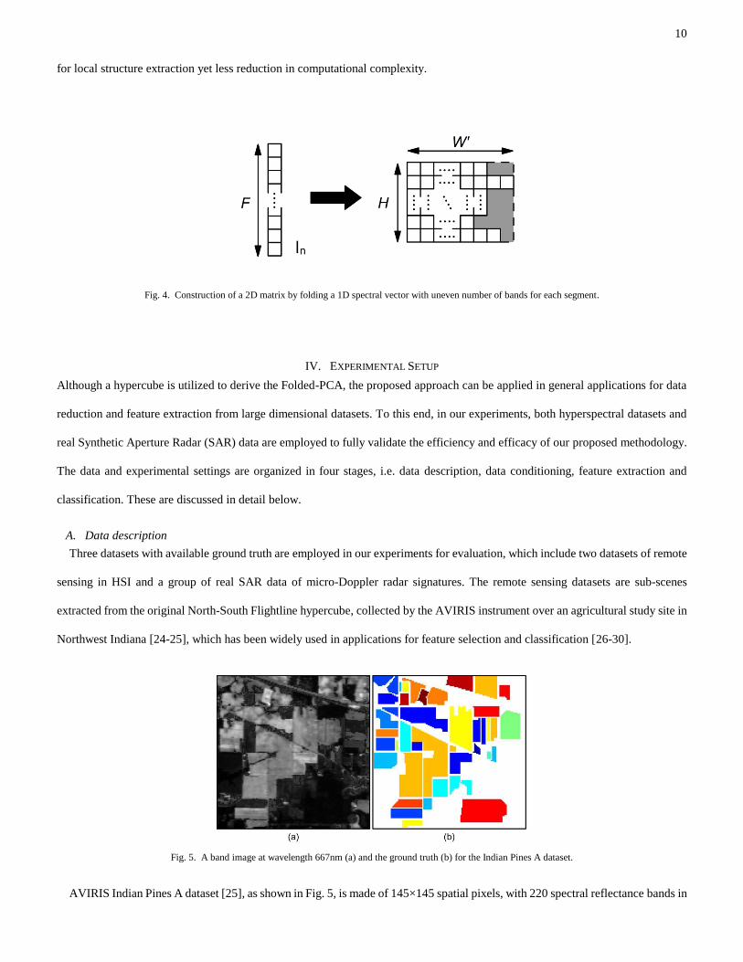
Fig. 5. A band image at wavelength 667nm (a) and the ground truth (b) for the Indian Pines A dataset.

AVIRIS Indian Pines A dataset [25], as shown in Fig. 5, is made of 145×145 spatial pixels, with 220 spectral reflectance bands in

11

the wavelength range 400-2500nm. It contains 16 land cover classes, presenting mostly agriculture, forest and natural perennial

vegetation.

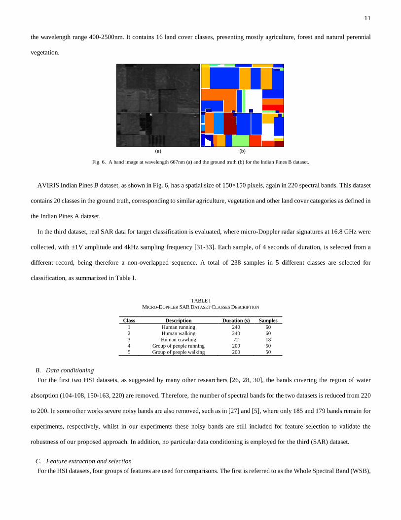
Fig. 6. A band image at wavelength 667nm (a) and the ground truth (b) for the Indian Pines B dataset.

AVIRIS Indian Pines B dataset, as shown in Fig. 6, has a spatial size of 150×150 pixels, again in 220 spectral bands. This dataset

contains 20 classes in the ground truth, corresponding to similar agriculture, vegetation and other land cover categories as defined in

the Indian Pines A dataset.

In the third dataset, real SAR data for target classification is evaluated, where micro-Doppler radar signatures at 16.8 GHz were

collected, with ±1V amplitude and 4kHz sampling frequency [31-33]. Each sample, of 4 seconds of duration, is selected from a

different record, being therefore a non-overlapped sequence. A total of 238 samples in 5 different classes are selected for

classification, as summarized in Table I.

TABLE I

MICRO-DOPPLER SAR DATASET CLASSES DESCRIPTION

Class Description Duration (s) Samples

1 Human running 240 60

2 Human walking 240 60

3 Human crawling 72 18

4 Group of people running 200 50

5 Group of people walking 200 50

B. Data conditioning

For the first two HSI datasets, as suggested by many other researchers [26, 28, 30], the bands covering the region of water

absorption (104-108, 150-163, 220) are removed. Therefore, the number of spectral bands for the two datasets is reduced from 220

to 200. In some other works severe noisy bands are also removed, such as in [27] and [5], where only 185 and 179 bands remain for

experiments, respectively, whilst in our experiments these noisy bands are still included for feature selection to validate the

robustness of our proposed approach. In addition, no particular data conditioning is employed for the third (SAR) dataset.

C. Feature extraction and selection

For the HSI datasets, four groups of features are used for comparisons. The first is referred to as the Whole Spectral Band (WSB),

12

in which the total 200 spectral bands are directly used as features for classification and evaluation. This is taken as a baseline

approach for benchmarking. The other three use principal components extracted as features, obtained from the conventional PCA,

our Folded-PCA, and the Segmented-PCA. In the Folded-PCA and Segmented-PCA cases, if not specified, the H and W

parameters used are 10 and 20, respectively.

For the SAR dataset, the Short Time Fourier Transform (STFT) is applied for feature extraction as follows. Let the input signal be

denoted as x , the transformed results form a matrix of complex values along both frequency and time dimensions represented in

R rows and C columns, respectively

RxCCtfSTFT ),(}{x (13)

By extracting the absolute value of these complex numbers, a group of 100 measurements as the Mean Frequency Profile (MFP)

over the time dimension is obtained [34]. Such frequency profile is a representative amount of data which make us able to

differentiate between targets. These 100 measurements are then used as features in our experiments for further feature selection

using the PCA, our Folded-PCA and Segmented-PCA approaches. The parameters H and W used here are 10 and 10

respectively

100

1)(,),(

1)(

fMFPtfSTFTT

fMFPT

t

(14)

D. Classification

For efficacy evaluation, the features obtained from feature extraction and feature selection are inputted to a standard Support

Vector Machine (SVM) for comparisons. The overall classification accuracy is taken as an objective measurement for quantitative

evaluation. The reasons to choose SVM are not only that it exploits a margin-based criterion and is very robust to the Hughes

phenomenon but also it has been widely used by many researchers in this field [26-30].

There are several libraries available for an easy SVM implementation, allowing even its use in embedded systems [35]. For

multi-class classification, one of the best external libraries, bSVM [36], is used for supervised learning allowing fast and accurate

modeling. The kernel utilized is gaussian Radial Basis Function (RBF), as it helps to produce good results in both HSI [26-27,

29-30] and SAR [37-38] applications. A total of 10 experiments are evaluated, where in every case, the training and testing samples

are randomly selected by stratified sampling, using an equal sample rate of 30% in each class for training the SVM model.

The parameters for the RBF kernel, the penalty (c) and the gamma (γ), are optimized every time by means of a grid search. From

each experiment the overall accuracy from the testing samples is obtained. Finally, the mean overall accuracy over the 10

experiments and its standard deviation are reported. Detailed results are presented and compared in the next Section V.

13

V. RESULTS AND EVALUATIONS

Using the experimental settings described in Section IV, several groups of results are generated and compared in this Section V for

performance assessment and evaluation of our proposed Folded-PCA approach. These are shown in three groups in terms of

reduction of computational cost, reduction of required memory and improvement of classification accuracy as detailed below.

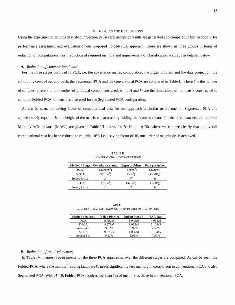
A. Reduction of computational cost

For the three stages involved in PCA, i.e. the covariance matrix computation, the Eigen problem and the data projection, the

computing costs of our approach, the Segmented-PCA and the conventional PCA are compared in Table II, where S is the number

of samples, q refers to the number of principal components used, while H and W are the dimensions of the matrix constructed to

compute Folded-PCA, dimensions also used for the Segmented-PCA configuration.

As can be seen, the saving factor of computational cost for our approach is similar to the one for Segmented-PCA and

approximately equal to H, the height of the matrix constructed by folding the features vector. For the three datasets, the required

Multiply-ACcumulates (MACs) are given in Table III below, for H=10 and q=30, where we can see clearly that the overall

computational cost has been reduced to roughly 10%, i.e. a saving factor of 10, one order of magnitude, is achieved.

TABLE II

COMPUTATIONAL COST COMPARISON

Method \ Stage Covariance matrix Eigen problem Data projection

PCA O(SH2W2) O(H3W3) O(SHWq)

F-PCA O(SHW2) O(W3) O(SWq)

Saving factor H H3 H

S-PCA O(SHW2) O(HW3) O(SWq)

Saving factor H H2 H

TABLE III

COMPUTATIONAL COST (MACS) FOR H=10 WITH 30 COMPONENTS

Method \ Dataset Indian Pines A Indian Pines B SAR data

PCA 9.752e8 1.043e9 4.094e6

F-PCA 9.672e7 1.035e8 3.104e5

Reduced to 9.92% 9.92% 7.58%

S-PCA 9.679e7 1.036e8 3.194e5

Reduced to 9.93% 9.93% 7.80%

B. Reduction of required memory

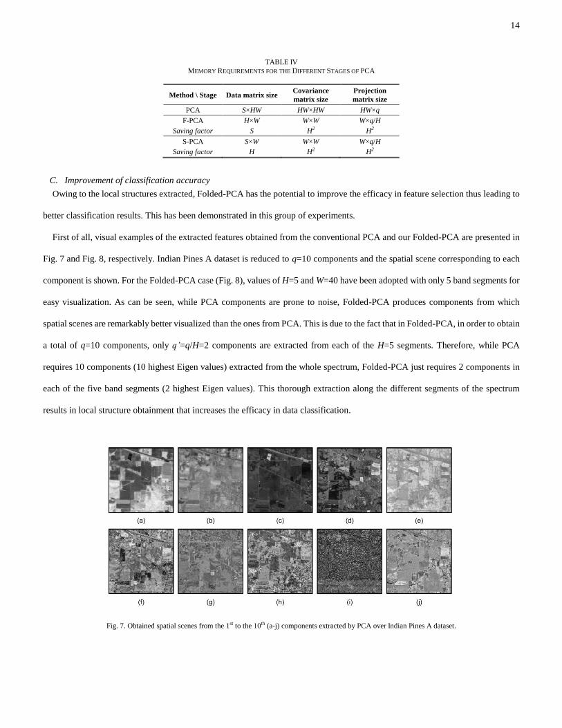
In Table IV, memory requirements for the three PCA approaches over the different stages are compared. As can be seen, the

Folded-PCA, where the minimum saving factor is H2, needs significantly less memory in comparison to conventional PCA and also

Segmented-PCA. With H=10, Folded-PCA requires less than 1% of memory as those in conventional PCA.

14

TABLE IV

MEMORY REQUIREMENTS FOR THE DIFFERENT STAGES OF PCA

Method \ Stage Data matrix size Covariance

matrix size

Projection

matrix size

PCA S×HW HW×HW HW×q

F-PCA H×W W×W W×q/H

Saving factor S H2 H2

S-PCA S×W W×W W×q/H

Saving factor H H2 H2

C. Improvement of classification accuracy

Owing to the local structures extracted, Folded-PCA has the potential to improve the efficacy in feature selection thus leading to

better classification results. This has been demonstrated in this group of experiments.

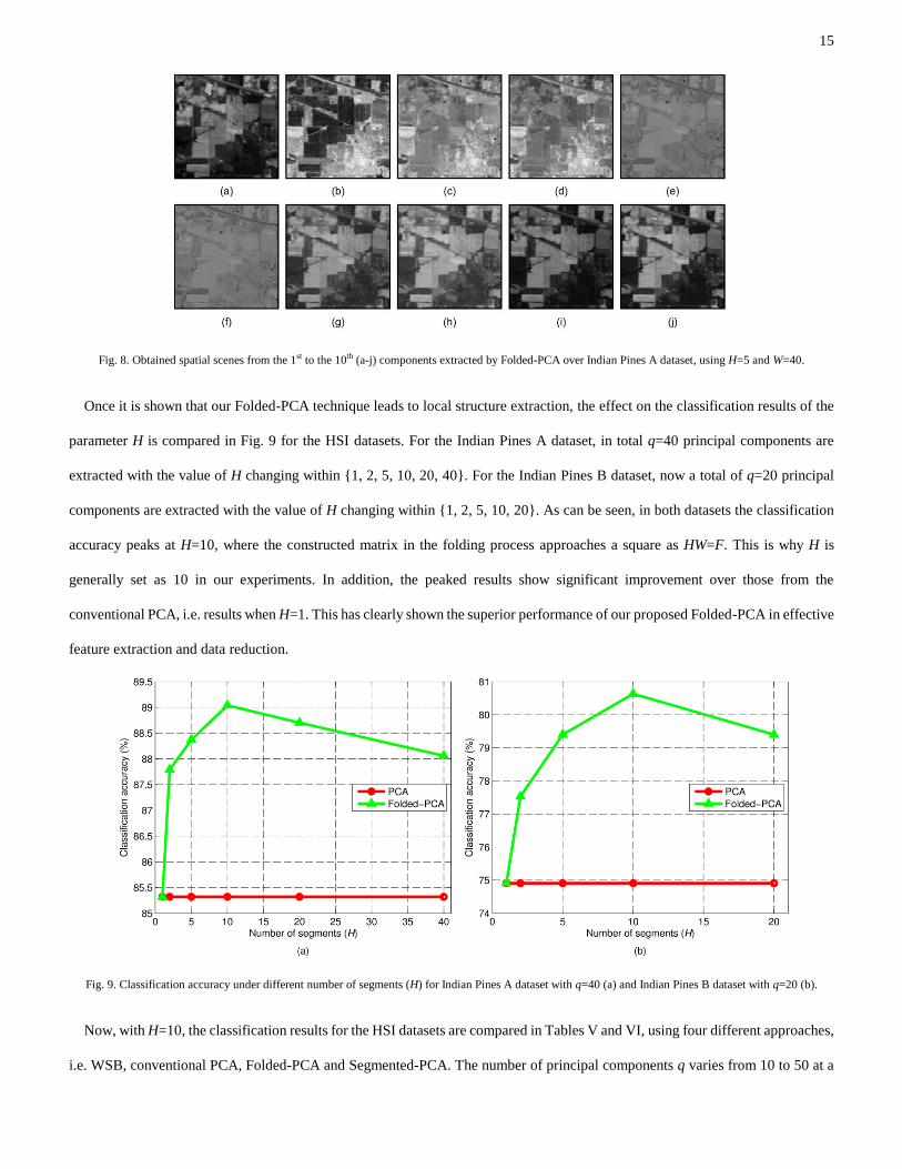
First of all, visual examples of the extracted features obtained from the conventional PCA and our Folded-PCA are presented in

Fig. 7 and Fig. 8, respectively. Indian Pines A dataset is reduced to q=10 components and the spatial scene corresponding to each

component is shown. For the Folded-PCA case (Fig. 8), values of H=5 and W=40 have been adopted with only 5 band segments for

easy visualization. As can be seen, while PCA components are prone to noise, Folded-PCA produces components from which

spatial scenes are remarkably better visualized than the ones from PCA. This is due to the fact that in Folded-PCA, in order to obtain

a total of q=10 components, only q’=q/H=2 components are extracted from each of the H=5 segments. Therefore, while PCA

requires 10 components (10 highest Eigen values) extracted from the whole spectrum, Folded-PCA just requires 2 components in

each of the five band segments (2 highest Eigen values). This thorough extraction along the different segments of the spectrum

results in local structure obtainment that increases the efficacy in data classification.

Fig. 7. Obtained spatial scenes from the 1st to the 10th (a-j) components extracted by PCA over Indian Pines A dataset.

15

Fig. 8. Obtained spatial scenes from the 1st to the 10th (a-j) components extracted by Folded-PCA over Indian Pines A dataset, using H=5 and W=40.

Once it is shown that our Folded-PCA technique leads to local structure extraction, the effect on the classification results of the

parameter H is compared in Fig. 9 for the HSI datasets. For the Indian Pines A dataset, in total q=40 principal components are

extracted with the value of H changing within {1, 2, 5, 10, 20, 40}. For the Indian Pines B dataset, now a total of q=20 principal

components are extracted with the value of H changing within {1, 2, 5, 10, 20}. As can be seen, in both datasets the classification

accuracy peaks at H=10, where the constructed matrix in the folding process approaches a square as HW=F. This is why H is

generally set as 10 in our experiments. In addition, the peaked results show significant improvement over those from the

conventional PCA, i.e. results when H=1. This has clearly shown the superior performance of our proposed Folded-PCA in effective

feature extraction and data reduction.

Fig. 9. Classification accuracy under different number of segments (H) for Indian Pines A dataset with q=40 (a) and Indian Pines B dataset with q=20 (b).

Now, with H=10, the classification results for the HSI datasets are compared in Tables V and VI, using four different approaches,

i.e. WSB, conventional PCA, Folded-PCA and Segmented-PCA. The number of principal components q varies from 10 to 50 at a

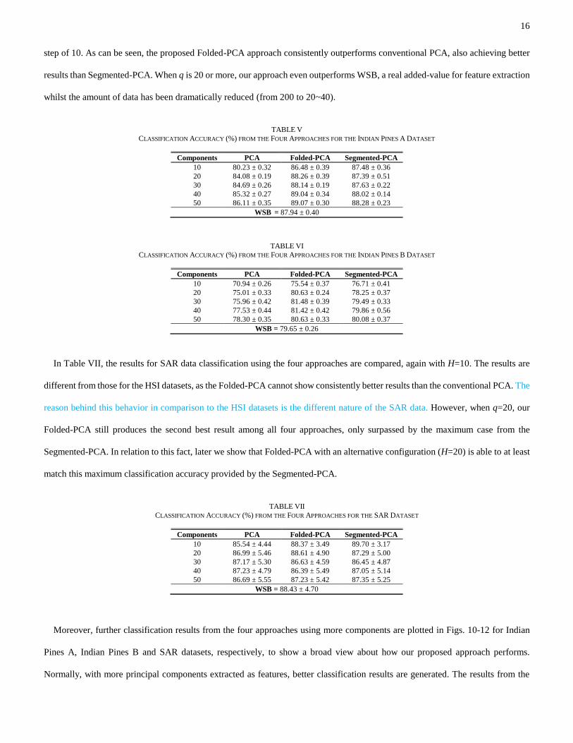
16

step of 10. As can be seen, the proposed Folded-PCA approach consistently outperforms conventional PCA, also achieving better

results than Segmented-PCA. When q is 20 or more, our approach even outperforms WSB, a real added-value for feature extraction

whilst the amount of data has been dramatically reduced (from 200 to 20~40).

TABLE V

CLASSIFICATION ACCURACY (%) FROM THE FOUR APPROACHES FOR THE INDIAN PINES A DATASET

Components PCA Folded-PCA Segmented-PCA

10 80.23 ± 0.32 86.48 ± 0.39 87.48 ± 0.36

20 84.08 ± 0.19 88.26 ± 0.39 87.39 ± 0.51

30 84.69 ± 0.26 88.14 ± 0.19 87.63 ± 0.22

40 85.32 ± 0.27 89.04 ± 0.34 88.02 ± 0.14

50 86.11 ± 0.35 89.07 ± 0.30 88.28 ± 0.23

WSB = 87.94 ± 0.40

TABLE VI

CLASSIFICATION ACCURACY (%) FROM THE FOUR APPROACHES FOR THE INDIAN PINES B DATASET

Components PCA Folded-PCA Segmented-PCA

10 70.94 ± 0.26 75.54 ± 0.37 76.71 ± 0.41

20 75.01 ± 0.33 80.63 ± 0.24 78.25 ± 0.37

30 75.96 ± 0.42 81.48 ± 0.39 79.49 ± 0.33

40 77.53 ± 0.44 81.42 ± 0.42 79.86 ± 0.56

50 78.30 ± 0.35 80.63 ± 0.33 80.08 ± 0.37

WSB = 79.65 ± 0.26

In Table VII, the results for SAR data classification using the four approaches are compared, again with H=10. The results are

different from those for the HSI datasets, as the Folded-PCA cannot show consistently better results than the conventional PCA. The

reason behind this behavior in comparison to the HSI datasets is the different nature of the SAR data. However, when q=20, our

Folded-PCA still produces the second best result among all four approaches, only surpassed by the maximum case from the

Segmented-PCA. In relation to this fact, later we show that Folded-PCA with an alternative configuration (H=20) is able to at least

match this maximum classification accuracy provided by the Segmented-PCA.

TABLE VII

CLASSIFICATION ACCURACY (%) FROM THE FOUR APPROACHES FOR THE SAR DATASET

Components PCA Folded-PCA Segmented-PCA

10 85.54 ± 4.44 88.37 ± 3.49 89.70 ± 3.17

20 86.99 ± 5.46 88.61 ± 4.90 87.29 ± 5.00

30 87.17 ± 5.30 86.63 ± 4.59 86.45 ± 4.87

40 87.23 ± 4.79 86.39 ± 5.49 87.05 ± 5.14

50 86.69 ± 5.55 87.23 ± 5.42 87.35 ± 5.25

WSB = 88.43 ± 4.70

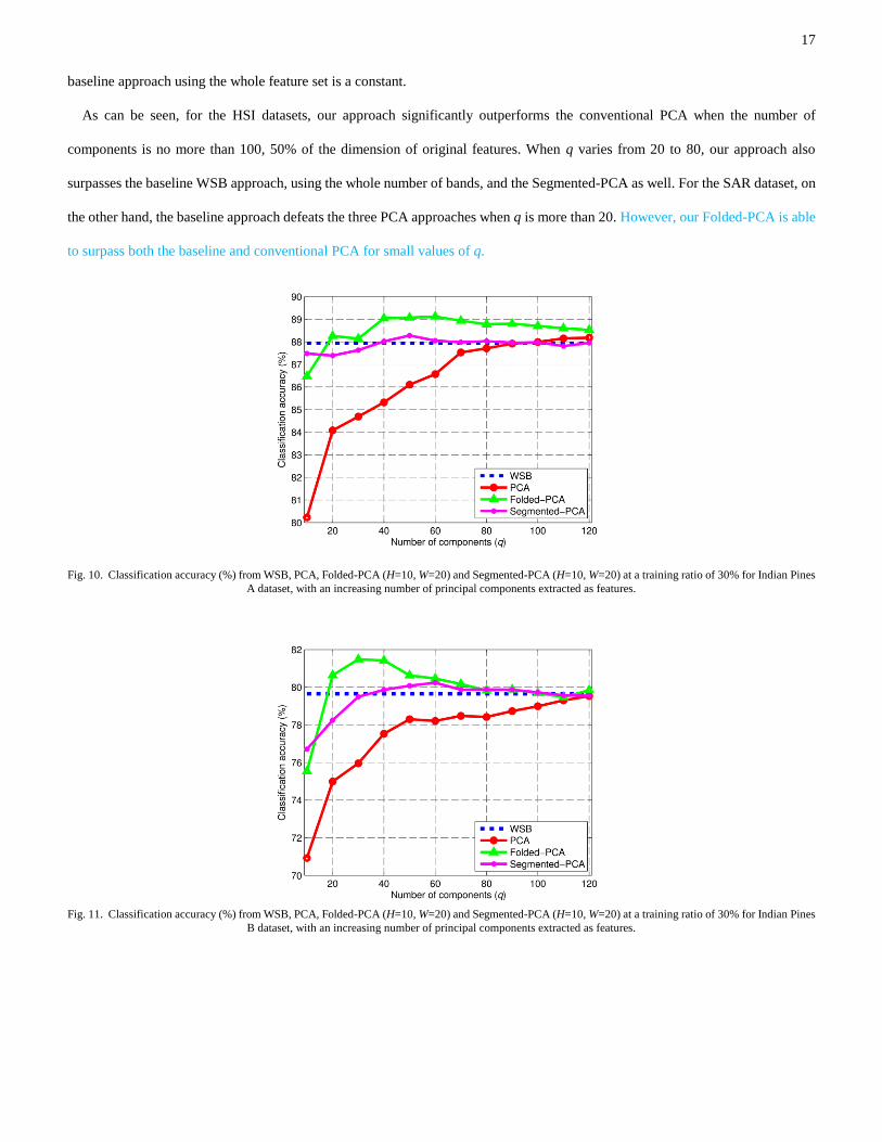
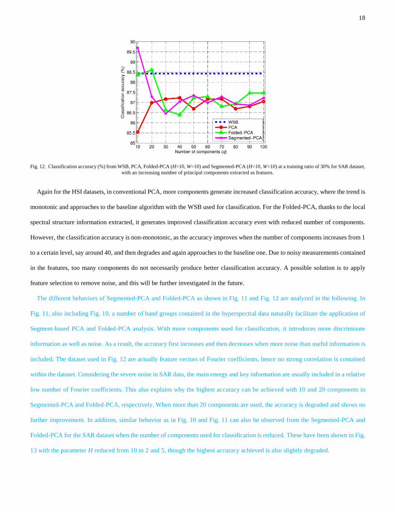
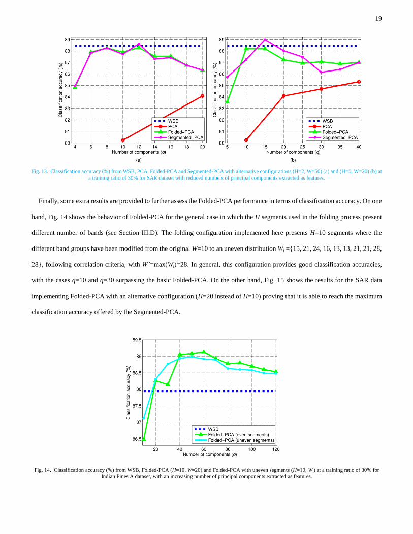
Moreover, further classification results from the four approaches using more components are plotted in Figs. 10-12 for Indian

Pines A, Indian Pines B and SAR datasets, respectively, to show a broad view about how our proposed approach performs.

Normally, with more principal components extracted as features, better classification results are generated. The results from the

17

baseline approach using the whole feature set is a constant.

As can be seen, for the HSI datasets, our approach significantly outperforms the conventional PCA when the number of

components is no more than 100, 50% of the dimension of original features. When q varies from 20 to 80, our approach also

surpasses the baseline WSB approach, using the whole number of bands, and the Segmented-PCA as well. For the SAR dataset, on

the other hand, the baseline approach defeats the three PCA approaches when q is more than 20. However, our Folded-PCA is able

to surpass both the baseline and conventional PCA for small values of q.

Fig. 10. Classification accuracy (%) from WSB, PCA, Folded-PCA (H=10, W=20) and Segmented-PCA (H=10, W=20) at a training ratio of 30% for Indian Pines

A dataset, with an increasing number of principal components extracted as features.

Fig. 11. Classification accuracy (%) from WSB, PCA, Folded-PCA (H=10, W=20) and Segmented-PCA (H=10, W=20) at a training ratio of 30% for Indian Pines

B dataset, with an increasing number of principal components extracted as features.

18

Fig. 12. Classification accuracy (%) from WSB, PCA, Folded-PCA (H=10, W=10) and Segmented-PCA (H=10, W=10) at a training ratio of 30% for SAR dataset,

with an increasing number of principal components extracted as features.

Again for the HSI datasets, in conventional PCA, more components generate increased classification accuracy, where the trend is

monotonic and approaches to the baseline algorithm with the WSB used for classification. For the Folded-PCA, thanks to the local

spectral structure information extracted, it generates improved classification accuracy even with reduced number of components.

However, the classification accuracy is non-monotonic, as the accuracy improves when the number of components increases from 1

to a certain level, say around 40, and then degrades and again approaches to the baseline one. Due to noisy measurements contained

in the features, too many components do not necessarily produce better classification accuracy. A possible solution is to apply

feature selection to remove noise, and this will be further investigated in the future.

The different behaviors of Segmented-PCA and Folded-PCA as shown in Fig. 11 and Fig. 12 are analyzed in the following. In

Fig. 11, also including Fig. 10, a number of band groups contained in the hyperspectral data naturally facilitate the application of

Segment-based PCA and Folded-PCA analysis. With more components used for classification, it introduces more discriminate

information as well as noise. As a result, the accuracy first increases and then decreases when more noise than useful information is

included. The dataset used in Fig. 12 are actually feature vectors of Fourier coefficients, hence no strong correlation is contained

within the dataset. Considering the severe noise in SAR data, the main energy and key information are usually included in a relative

low number of Fourier coefficients. This also explains why the highest accuracy can be achieved with 10 and 20 components in

Segmented-PCA and Folded-PCA, respectively. When more than 20 components are used, the accuracy is degraded and shows no

further improvement. In addition, similar behavior as in Fig. 10 and Fig. 11 can also be observed from the Segmented-PCA and

Folded-PCA for the SAR dataset when the number of components used for classification is reduced. These have been shown in Fig.

13 with the parameter H reduced from 10 to 2 and 5, though the highest accuracy achieved is also slightly degraded.

19

Fig. 13. Classification accuracy (%) from WSB, PCA, Folded-PCA and Segmented-PCA with alternative configurations (H=2, W=50) (a) and (H=5, W=20) (b) at

a training ratio of 30% for SAR dataset with reduced numbers of principal components extracted as features.

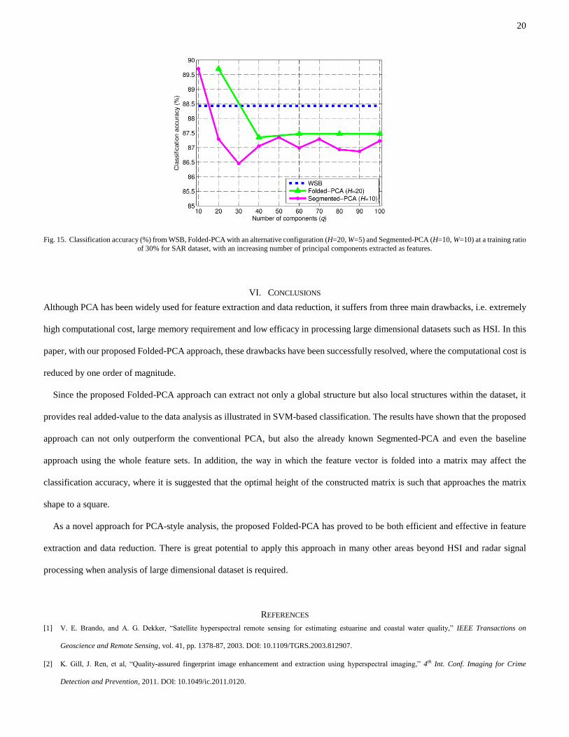
Finally, some extra results are provided to further assess the Folded-PCA performance in terms of classification accuracy. On one

hand, Fig. 14 shows the behavior of Folded-PCA for the general case in which the H segments used in the folding process present

different number of bands (see Section III.D). The folding configuration implemented here presents H=10 segments where the

different band groups have been modified from the original W=10 to an uneven distribution Wi ={15, 21, 24, 16, 13, 13, 21, 21, 28,

28}, following correlation criteria, with W’=max(Wi)=28. In general, this configuration provides good classification accuracies,

with the cases q=10 and q=30 surpassing the basic Folded-PCA. On the other hand, Fig. 15 shows the results for the SAR data

implementing Folded-PCA with an alternative configuration (H=20 instead of H=10) proving that it is able to reach the maximum

classification accuracy offered by the Segmented-PCA.

Fig. 14. Classification accuracy (%) from WSB, Folded-PCA (H=10, W=20) and Folded-PCA with uneven segments (H=10, Wi) at a training ratio of 30% for

Indian Pines A dataset, with an increasing number of principal components extracted as features.

20

Fig. 15. Classification accuracy (%) from WSB, Folded-PCA with an alternative configuration (H=20, W=5) and Segmented-PCA (H=10, W=10) at a training ratio

of 30% for SAR dataset, with an increasing number of principal components extracted as features.

VI. CONCLUSIONS

Although PCA has been widely used for feature extraction and data reduction, it suffers from three main drawbacks, i.e. extremely

high computational cost, large memory requirement and low efficacy in processing large dimensional datasets such as HSI. In this

paper, with our proposed Folded-PCA approach, these drawbacks have been successfully resolved, where the computational cost is

reduced by one order of magnitude.

Since the proposed Folded-PCA approach can extract not only a global structure but also local structures within the dataset, it

provides real added-value to the data analysis as illustrated in SVM-based classification. The results have shown that the proposed

approach can not only outperform the conventional PCA, but also the already known Segmented-PCA and even the baseline

approach using the whole feature sets. In addition, the way in which the feature vector is folded into a matrix may affect the

classification accuracy, where it is suggested that the optimal height of the constructed matrix is such that approaches the matrix

shape to a square.

As a novel approach for PCA-style analysis, the proposed Folded-PCA has proved to be both efficient and effective in feature

extraction and data reduction. There is great potential to apply this approach in many other areas beyond HSI and radar signal

processing when analysis of large dimensional dataset is required.

REFERENCES

[1] V. E. Brando, and A. G. Dekker, “Satellite hyperspectral remote sensing for estimating estuarine and coastal water quality,” IEEE Transactions on

Geoscience and Remote Sensing, vol. 41, pp. 1378-87, 2003. DOI: 10.1109/TGRS.2003.812907.

[2] K. Gill, J. Ren, et al, “Quality-assured fingerprint image enhancement and extraction using hyperspectral imaging,” 4th Int. Conf. Imaging for Crime

Detection and Prevention, 2011. DOI: 10.1049/ic.2011.0120.

21

[3] G. Hughes, “On the mean accuracy of statistical pattern recognizers,” IEEE Transactions on Information Theory, vol. 14, no. 1, pp. 55–63, January 1968.

DOI: 10.1109/TIT.1968.1054102.

[4] S. Wang, and C.-I. Chang, “Variable-number variable-band selection for feature characterization in hyperspectral signatures,” IEEE Trans Geoscience and

Remote Sensing, 45(9): 2979-2992, Sept. 2007. DOI: 10.1109/TGRS.2007.901051.

[5] R. Dianat, and S. Kasaei, “Dimension reduction of optical remote sensing images via minimum change rate deviation method,” IEEE Trans Geoscience and

Remote Sensing, 48(1): 198-206, Jan. 2010. DOI: 10.1109/TGRS.2009.2024306.

[6] M. He, and S. Mei, “Dimension reduction by random projection for endmember extraction,” in Proc. IEEE Conf. Ind. Electron. Appl., pp. 2323–2327, June

2010. DOI: 10.1109/ICIEA.2010.5516724.

[7] R. D. Phillips, W. T. Watson, R. H. Wynne, and C. E. Blinn, “Feature reduction using a singular value decomposition for the iterative guided spectral class

rejection hybrid classifier,” ISPRS J. Photogramm. Remote Sensing, vol. 64, no. 1, pp. 107–116, January 2009. DOI: 10.1016/j.isprsjprs.2008.03.004.

[8] A. Green, M. Berman, P. Switzer, and M. Craig, “A transformation for ordering multispectral data in terms of image quality with implications for noise

removal,” IEEE Transactions on Geoscience and Remote Sensing, vol. 26, no. 1, pp. 65–74, 1988. DOI: 10.1109/36.3001.

[9] H. Abdi, and L. J. Williams, Principal component analysis, Wiley Interdisciplinary Reviews: Computational Statistics, 2010. DOI: 10.1002/wics.101.

[10] Q. Du, and J. Fowler, “Hyperspectral image compression using JPEG2000 and principal component analysis,” IEEE Geoscience and Remote Sensing Letters,

vol. 4, no. 2, pp. 201-205, 2007. DOI: 10.1109/LGRS.2006.888109.

[11] J. Qin, T.F. Burks, M.S. Kim, K. Chao, and M.A. Ritenour, “Citrus canker detection using hyperspectral reflectance imaging and PCA-based image

classification method,” Sensing and Instrumentation for Food Quality and Safety, vol. 2, no. 3, pp. 168-177, 2008. DOI: 10.1007/s11694-008-9043-3.

[12] R. Archibald, and G. Fann. “Feature selection and classification of hyperspectral images with support vector machines,” IEEE Geoscience and Remote

Sensing Letters, vol. 4, no. 4, pp. 674-677, October 2007. DOI: 10.1109/LGRS.2007.905116.

[13] C. Wang, L. Pasteur, M. Menenti, and Z-L Li, “Modified principal component analysis (mpca) for feature selection of hyperspectral imagery,” in Geoscience

and Remote Sensing Symposium (IGARSS), vol. 6, pp. 3781-3783, July 2003. DOI: 10.1109/IGARSS.2003.1295268.

[14] P. Hall, and R. Martin, “Incremental eigenanalysis for classification,” in Proceedings of the British Machine Vision Conference, vol. 1, pp. 286-295, 1998.

DOI: 10.5244/C.12.29.

[15] X. Jia, and J.A. Richards, “Segmented principal components transformation for efficient hyperspectral remote sensing image display and classification,”

IEEE Trans. on Geoscience and Remote Sensing, vol. 37, pp. 538-542, 1999. DOI: 10.1109/36.739109.

[16] J. Yang, D. Zhang, A. F. Frangi, and J-Y Yang, “Two-Dimensional pca: A new approach to appearance-based face representation and recognition,” IEEE

Transactions on Pattern Analysis and Machine Intelligence, vol. 26, no.1, pp. 131-137, January 2004. DOI: 10.1109/TPAMI.2004.1261097.

[17] D. Zhang, and Z-H. Zhou, “(2d)2 PCA: 2-directional 2-dimensional PCA for efficient face representation and recognition,” Journal of Neurocomputing, vol.

69, no. 1-3, pp. 224-231, December 2005. DOI: 10.1016/j.neucom.2005.06.004.

[18] Y. Zeng, D. Feng, and L. Xiong, “An algorithm of face recognition based on the variation of 2DPCA,” Journal of Computational Information Systems, vol.

7, no. 1 pp. 303-310, January 2011.

[19] H. Kong, L. Wang, E. K. Teoh, X. Li, J-G. Wang, and R. Venkateswarlu, “Generalized 2D principal component analysis for face image representation and

recognition,” Neural Networks, Elsevier, vol. 18, pp. 585–594, 2005. DOI: 10.1016/j.neunet.2005.06.041.

[20] L. Wang, X. Wang, X. Zhang and J. Feng, “The equivalence of two-dimensional pca to line-based pca,” Pattern Recognition Letters, Elsevier, vol. 26 pp.

57–60, 2005. DOI: 10.1016/j.patrec.2004.08.016.

22

[21] Y. Zhao, L. Zhang, and S. Kong, “Band-subset-based clustering and fusion for hyperspectral imagery classification,” IEEE Trans. Geoscience and Remote

Sensing, vol. 49, no. 2, pp. 747-756, 2011. DOI: 10.1109/TGRS.2010.2059707.

[22] E. Pang, S. Wang, M. Qu, et al, “2D-SPP: a two-dimensional extension of sparsity preserving projections,” Journal of Information and Computational

Science, vol. 9, no. 13, pp. 3683-3692, 2012.

[23] S. Yu, J. Bi, and J. Ye, “Probabilistic interpretations and extensions for a family of 2D PCA-style algorithms,” In Proc. The KDD’2008 workshop on Data

Mining using Matrices and Tensors, 2008.

[24] “Pursue's univeristy multispec site: June 12, 1992 aviris image north-south flightline, indiana,” [Online]. Available: https://engineering.purdue.edu/~biehl/

MultiSpec/hyperspectral.html

[25] “Hyperspectral Remote Sensing Scenes,” [Online]. Available: http://www.ehu.es/ccwintco/index.php/Hyperspectral_Remote_Sensing_Scenes

[26] F. Melgani, and L. Bruzzone, “Classification of hyperspectral remote sensing images with support vector machines,” IEEE Trans. Geoscience and Remote

Sensing, vol. 42, no. 8, pp. 1778–1790, August 2004. DOI: 10.1109/TGRS.2004.831865.

[27] M. Pal, and G. M. Foody, “Feature selection for classification of hyperspectral data by SVM,” IEEE Transactions on Geoscience and Remote Sensing, vol.

48, no. 5, pp. 2297-2307, May 2010. DOI: 10.1109/TGRS.2009.2039484.

[28] H. Huang, J. Liu, and Y. Pan, “Semi-supervised marginal fisher analysis for hyperspectral image classification,” ISPRS Annals of the Photogrammetry,

Remote Sensing and Spatial Information Sciences, Volume I-3, XXII ISPRS Congress, 2012. DOI: 10.5194/isprsannals-I-3-377-2012.

[29] M. Rojas, I. D´opido, A. Plaza, and P. Gamba, “Comparison of support vector machine-based processing chains for hyperspectral image classification,” in

Proceedings of SPIE, vol. 7810, 2010. DOI: 10.1117/12.860413.

[30] G. Camps-Valls, and L. Bruzzone, “Kernel-based methods for hyperspectral image classification,” IEEE Trans. Geosci. Remote Sens, vol. 43, no. 6, pp.

1351–1362, Jun. 2005. DOI: 10.1109/TGRS.2005.846154.

[31] “The database of radar echoes from various targets,” [Online]. Available: http://cid-3aaf3e18829259c0.skydrive.live.com/home.aspx

[32] M. Andric, B. Bondzulic, and B. Zrnic, “The database of radar echoes from various targets with spectral analysis,” in 10th Symposium on Neural Network

Applications in Electrical Engineering (NEUREL), Serbia, September, pp.187-190, 2010. DOI: 10.1109/NEUREL.2010.5644074.

[33] M. Andric, B. Bondzulic, and B. Zrnic, “Feature extraction related to target classification for a radar doppler echoes,” in 18th Telecommunications Forum

TELFOR, Serbia, November, 2010.

[34] J. Zabalza, C. Clemente, G. Di Caterina, J. Ren, J. J. Soraghan, and S. Marshall, “Robust pca micro-doppler classification using svm on embedded systems,”

IEEE Transactions on Aerospace and Electronic Systems (in Press).

[35] J. Zabalza, J. Ren, C. Clemente, G. Di Caterina, and J. J. Soraghan, “Embedded svm on tms320c6713 for signal prediction in classification and regression

applications,” in 5th European DSP Education and Research Conf., Amsterdam, Sept. 2012. DOI: 10.1109/EDERC.2012.6532232.

[36] “bSVM multiclass classifier 2.08,” released on June 18, 2012 [Online]. Available: http://www.csie.ntu.edu.tw/~cjlin/bsvm/

[37] Y. Kim, and H. Ling, “Human activity classification based on microdoppler signatures using a support vector machine,” IEEE Trans. Geoscience and Remote

Sensing, vol. 47, no. 5, pp. 1328–1337, 2009. DOI: 10.1109/TGRS.2009.2012849.

[38] P. Molchanov, J. Astola, K. Egiazarian, and A. Totsky, “Classification of ground moving radar targets by using joint time-frequency analysis,” in IEEE 2012

Radar Conference, pp. 0366-0371, May 2012. DOI: 10.1109/RADAR.2012.6212166.