| bonorowo wetlands | vol. 8 | no. 1 | june 2018 | issn
TRANSCRIPT
| Bonorowo Wetlands | vol. 8 | no. 1 | June 2018 | ISSN 2088-110X | E-ISSN 2088-2475|
Eich
ho
rnia
cra
ssip
es p
ho
to b
y Y
oyo
h

| Bonorowo Wetlands | vol. 8 | no. 1 | June 2018 |
ONLINE
http://smujo.id/bw
p-ISSN: 2088-110X, e-ISSN: 2088-2475
PUBLISHER
Society for Indonesian Biodiversity
CO-PUBLISHER
Institut Pertanian Bogor, Bogor, Indonesia
Nusantara Institut of Biodiversity, Universitas Sebelas Maret, Surakarta, Indonesia
OFFICE ADDRESS
1. Forest and Land Fire Laboratory, Department of Silviculture, Faculty of Forestry, Institut Pertanian Bogor.
Jl. Lingkar Akademik Kampus IPB Dramaga, Bogor 16680, West Java, Indonesia. Tel.: +62 251 8626806, Fax.: +62 251 8626886;
2. Department of Biology, Faculty of Mathematics and Natural Sciences, Universitas Sebelas Maret.
Jl. Ir. Sutami 36A Surakarta 57126, Central Java, Indonesia. Tel./Fax.: +62-271-663375,
email: [email protected], [email protected]
PERIOD OF ISSUANCE
June, December
EDITOR-IN-CHIEF
Bambang Hero Saharjo – Institut Pertanian Bogor, Bogor, Indonesia
ASSOCIATE EDITOR
Ahmad Dwi Setyawan – Universitas Sebelas Maret, Surakarta, Indonesia
EDITORIAL BOARD
Abd Fattah N. Abd Rabou – Islamic University of Gaza, Palestine
Abdul Malik – Universitas Negeri Makassar, Makassar, Indonesia
Alireza Naqinezhad – University of Mazandaran, Babolsar, Iran
Am A. Taurusman – Institut Pertanian Bogor, Bogor, Indonesia
Analuddin – Universitas Halu Oleo, Kendari, Indonesia
Cecep Kusmana – Institut Pertanian Bogor, Bogor, Indonesia
Gusti Z. Anshari – Universitas Tanjungpura, Pontianak, Indonesia
Heru Kuswantoro – Indonesian Legumes and Tuber Crops Research Institute (ILETRI), Malang, Indonesia
Indrastuti A. Rumanti – Indonesian Center for Rice Research (ICRR), Sukamandi, Subang, Indonesia
Mohamed O. Arnous – Suez Canal University, Ismailia, Egypt
Muhammad A. Rifa’i – Universitas Lambung Mangkurat, Banjarbaru, Indonesia
Onrizal – Universitas Sumatera Utara, Medan, Indonesia
Sk. Alamgir Badsha – University of Burdwan, Burdwan, India
Sudarmadji – Universitas Negeri Jember, Indonesia
Sunarto – Universitas Sebelas Maret, Surakarta, Indonesia
Syarifuddin – Universitas Negeri Medan, Medan, Indonesia
Tamires Soares Yule – Universidade Federal de Mato Grosso do Sul, Brazil
Udhi E. Hernawan – Research Center for Oceanography, Indonesian Institute of Sciences, Tual, Indonesia
EDITORIAL MEMBER Alfin Widiastuti – Development Agency for Seed Quality Testing of Food and Horticulture Crops, Depok, Indonesia
Society for Indonesian Biodiversity
Universitas Sebelas Maret Surakarta, Indonesia
Institut Pertanian Bogor, Bogor, Indonesia

BONOROWO WETLANDS P-ISSN: 2088-110X Volume 8, Number 1, June 2018 E-ISSN: 2088-2475
Pages: 1-12 DOI: 10.13057/bonorowo/w080101
Diversity and distribution of vascular macrophytes in Ansupa Lake,
Odisha, India
MUKTIPADA PANDA1,2,, RABINDRO NATH SAMAL1, KRUPA SINDHU BHATTA1, SASMITA LENKA1,
JAJNASENI ROUT1, HEMANTA KUMAR PATRA2, SUSANTA NANDA1
1Chilika Development Authority, Department of Forest and Environment, Govt. of Odisha, Plot No. C-11, BJB Nagar, Bhubaneswar 751014,
Odisha, India. email: [email protected] 2Post-Graduate Department of Botany, Utkal University. Bhubaneswar 751004, Odisha, India
Manuscript received: 14 March 2018. Revision accepted: 17 May 2018.
Abstract. Panda M, Samal RN, Bhatta KS, Lenka S, Rout J, Patra HK, Nanda S. 2018. Diversity and distribution of vascular
macrophytes in Ansupa Lake, Odisha, India. Bonorowo Wetlands 1: 1-12. Macrophytes are indispensable component of any wetlands.
They are the base of the trophic structure and variously affect function of aquatic ecosystem. Large invasion of macrophytes enforced
for present studies in Ansupa Lake, the largest freshwater lake of the state Odisha (India) to identify the causative plant species. Regular
field inspection, quadratic sampling and specimen collections were carried to identify the present macrophytes of the lake and their
quantitative aspects like frequency of occurrences, abundance, values of diversity indices, adaptation and growth forms and species
distribution etc. A total of 244 macrophyte species were identified that includes 182 semi-aquatic and 62 obligatory aquatic
macrophytes. The latter group had 35% submerged, 15% free floating, 31% rooted floating and 19% marshy plant species. The
comparison of growth form showed 66% annuals and remaining 34% perennial plants. The diversity indices resulted, Simpson
complement index-0.561, Shannon-Weiner index-1.367, Species richness index 3.079 and Species evenness index-0.156. The study
showed that the lake provides suitable habitats for existence of a diverse group of macrophytes but still due to large invasion of few
species has threatened the lake which needs to be managed properly to restore the health of this natural resource for the benefit of
mankind.
Keywords: Ansupa Lake, conservation, macrophyte diversity, species invasion
INTRODUCTION
Wetlands are the hotspots of biological diversity and
invaluable for sustainable living. Plants in water are called
macrophytes (Dodds 2002). They act as ‘‘biological
engineers’’ in restoring water quality (Byers et al. 2006). It
includes both flowering and non-flowering plants that start
their life in and around water bodies (Chambers et al.
2008). A total of 2614 aquatic vascular macrophytes occur
globally which represent only 1% of the total number of
vascular plants (Ansari et al. 2017). Total number of
aquatic plant species in Indian freshwaters exceeds 1200
(Gopal 1995). Many species of aquatic plant are invasive
species (Oyedeji and Abowei 2012). These plants cause
local losses of species diversity and alter ecosystem
structure, resulting in a significant negative impact on
aquatic biodiversity and water quality (Brundu 2015;
Chamier et al. 2012; Wang et al. 2016; Zedler and Kercher
2004). In India, over 140 aquatic plants are reported to
have attained the status of aquatic weeds in different
situations (Gupta 2012; Naskar 1990; Shah and Reshi
2012; Varshney et al. 2008).
Ansupa Lake, the present study sites is the largest fresh
water lake of the state Odisha (India) (Mohanty and Das
2008) and a lake of national importance (Das and Mohanty
2008). The lake provides livelihood provisions like fishing
i.e., small indigenous fishes, table size fishes and
ornamental fishes; agriculture, i.e., rice cultivation; edible
aquatic plants and ecotourism due to its unique biodiversity
and natural scenery (Sarkar et al. 2015). More than 25,000
fishermen and local residence make their livelihood on the
lake water (Das and Mohanty 2008; Mohanty and Das
2008). The average water depth of the lake was 4 meters
(Das and Mohanty 2008). The lake receives annual rainfall
between 800mm to 1300mm (Das and Mohanty 2008;
Panda et al. 2016) and most during months of July and
August, each year. It hosts 44 species of phytoplankton, 32
species of zooplanktons and 30 species of fishes (Patra and
Patra 2007). Panda et al. (2016) for the first time reported
occurrence of Hygroryza aristata (Retz.) Nees. ex Wt. and
Arn., a wild relative of edible rice in Ansupa Lake as the
only habitat in the state for this species. There is few
published work on Ansupa Lake and the macrophytes study
is very poorly reported (Das and Mohanty 2008; Mohanty
and Das 2008; Varshney et al. 2008; Sarkar et al. 2015;
Panda et al. 2016). All previous studies reported the
progressive degradation conditions of the lake due to
siltation, shrinkage of water spread area and invasions of
aquatic plants (Das and Mohanty 2008; Mohanty and Das
2008; Sarkar et al. 2015; Panda et al. 2016).
Knowing the importance of Ansupa Lake, present
studies were designed to identify the macrophyte diversity,
the problematic weeds that need to be managed properly
for the long term conservation of indigenous biota and
creation of better livelihood opportunity from the lake.

BONOROWO WETLANDS 8 (1): 1-12, June 2018
2
MATERIALS AND METHODS
Study area
Ansupa Lake is the largest fresh water lake of Odisha
State, India, situated between latitude 20 26 21 to 20
28 52 N and 85 36 25 to 85 36 0 E longitude on the
river bank of Mahanadi (Figure 1). The area of the lake is
around 375 acres and 385 acres during the dry and rainy
seasons, respectively (Mohanty and Das 2008).
Field data collection and floristic study
The floristic studies were carried during November
2014 and an extensive regular field work from April to
November 2017. The recorded macrophytes were
identified with the help of available both regional and
international scientific literatures (Calvert and Liessmann
2014; Campbell et al. 2010; Crow and Hellquist 2000; Das
2012; Gerber et al. 2004; Ghosh 2005; Gupta 2012; Haines
1921-1925; Naskar 1990). The scientific name and author
citation were checked with, The plant list
(http://www.theplantlist.org/) and International Plant Names
Index (http://www.ipni.org/ipni/plantnamesearchpage.do).
Quantitative status and ecological parameters were
calculated from 25 fixed random plots, i.e. size, 1m 1m
(Figure 1).
Data analysis
The quadratic parameters like, Frequency and
Abundance (Upadhyay et al. 2009), Whitford’s index (A/F)
(Whitford 1949), Species richness index (Margalef 1958),
Simpson complement index (1-DS) from Simpson
Dominance index (Simpson 1949), Shannon-Wiener index
(Shannon and Wiener 1963) and Species evenness index (J)
(Pielou 1975) were calculated as follows:
Where, S is the total number of species in the
community and N is the total number of individuals of all
species of a community.
Figure 1. Location map of Ansupa Lake, Cuttack District, Odisha, India

PANDA et al. – Macrophyte diversity of Ansupa Lake, Odisha, India
3
Where,
Where, H is the Shannon-Weiner index of the community
and S is the total number of species in the community.
RESULTS AND DISCUSSION
A total of 244 vascular macrophytes were identified to
occur in and shoreline areas of the lake. Out of the total
record, 238 species were of flowering plants, i.e.,
Angiosperms (Table 1) and 6 species of non-flowering
macrophytes, i.e., Pteridophyte (Table 2). All six
pteridophytes were strictly aquatic species; they belong to
only two families (i.e., Marsileaceae and Salviniaceae) and
except Azolla microphylla Kaulf., which was an annual
species others were perennial in their growth form (Table
2). The angiospermic macrophytes belong to a total of sixty
families. Among these families, Poaceae and Cyperaceae
were recorded as the most diversified families (Figure 2).
The classification of all the recorded macrophytes on the
basis of habitat preference showed 182 (75%) semi-aquatic
species and 62 (25%) aquatic species (Figure 3).
Categorization of total angiosperms revealed 137 (58%)
dicot species and 101 (42%) monocot species (Figure 4).
Among the dicot group, only 26 (19%) species were strictly
aquatic and 111 (81%) species were semi-aquatic plants
(Figure 5). Similarly, the monocot group had 30 species
(30%) and 71 species (70%) as aquatic and semi-aquatic
plants, respectively (Figure 6). The comparison of growth
form showed 160 species (66%) annual and remaining 84
species (34%) as perennial macrophytes (Figure 7). The
classification of total aquatic species displayed 35%
submerged, 15% free floating, 31% rooted floating and
19% marshy plant species (Figure 8). The study of nativity
resulted 56 species out of 244 species as exotic or non
native macrophytes of India (Table 1 and Table 2).
Quadratic study revealed quantitative status of twenty eight
common macrophytes (Table 3). Maximum species
diversity was recorded in the peripheral or shoreline plots.
Most frequent and abundant species were Ceratophylum
demersum L., Hydrila verticelastar (L.) Pers., Nelumbo
nucefera Gaertn., Najas sp., Utricularia sp.,Eichhornia
crassipes (Mart.) Solm-Laub. and Salvinia molesta D. S.
Mitch from interior of the lake. Other species like,
Polygonum barbatum L., Hymenachne amplexicaulis
(Rudge) Nees, Cyperus iria L., Alternanthera
philoxeroides A. St-Hil., Cyperus rotundus L. were more
abundant at the land water interface (i.e., marshy areas).
The distribution pattern (i.e. Whitford’s index) showed all
species with more or less of contagious type of distribution
(A/F 0.05). The diversity indices study showed Simpson
complement index-0.561, Shannon-Weiner index-1.367,
Species richness index 3.079 and Species evenness index-
0.156 (Figure 9).
Figure 2. Family wise recorded number of angiospermic
macrophytes species
The study found occurrence of wide habitat variability
that helped establishment of different group of aquatic and
semi-aquatic vascular macrophytes in the lake. Many
macrophytes showed seasonal changes of population status,
influenced by water level (Dalu et al. 2012). This affects
the value of diversity index of the ecosystem, as calculated
by ratio between the number of species and the number of
individuals in that community (Ansari et al. 2017). The low
value of species evenness index showed the present species
were not equally abundant, some species dominated over
others. The lake hosts some unique macrophytes that found
rarely elsewhere in the state. Hygroryza aristata (Retz.)
Nees. Ex Wt. & Arn. and Oryza rufipogon Griff., the wild

BONOROWO WETLANDS 8 (1): 1-12, June 2018
4
Figure 3. Classification as per habitat requirement: Aquatic and
semi-aquatic plants (%)
Figure 4. Classification into Angiosperm group: Diversity of
dicot and monocot species (%)
Figure 5. Classification of dicots into habitat group: Aquatic and
semi-aquatic dicots (%)
Figure 6. Classification of monocots into habitat groups: Aquatic
and semi-aquatic monocots (%)
Figure 7. Classification of macrophytes into growth forms:
Growth form of macrophytes (%)
Figure 8. Classification of aquatic plants into their adaptation
group: Adaptation forms of aquatic plants (%)
relative of edible rice were a common occurrence in the
lake (Plate 1). The aesthetically important and endangerd
plant species, Gloriosa superba L. has been recorded from
shoreline areas of the lake for the first time (Plate 1). The
semi-aquatic plants were diverse and many showed
seasonal growth. Many of them were small herbaceous
annual plants.
Strong infestation of Nelumbo nucifera Gaertn.,
Eichhornia crassipes (Mart.) Solm-Laub., Salvinia molesta
D. S. Mitch, Ceratophyllum demersum L., Hydrilla
verticillata (L.f.) Royle, Najas indica (Willd) Cham.;
Hymenachne amplexicaulis (Rudge) Nees, other grasses
and marshy vegetation were found negatively affecting the
lake (Plate 2). Soil erosion from surrounded hills and
siltation, decreased water flow due to closing of inlets and
outlets with Mahanadi River, intensive fertilizer load are
the possible factors for degradation of the lake.
Figure 9. Diversity indices from quadrate data
PANDA et al. – Macrophyte diversity of Ansupa Lake, Odisha, India
5
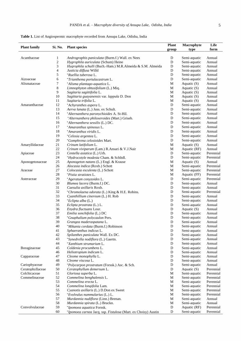
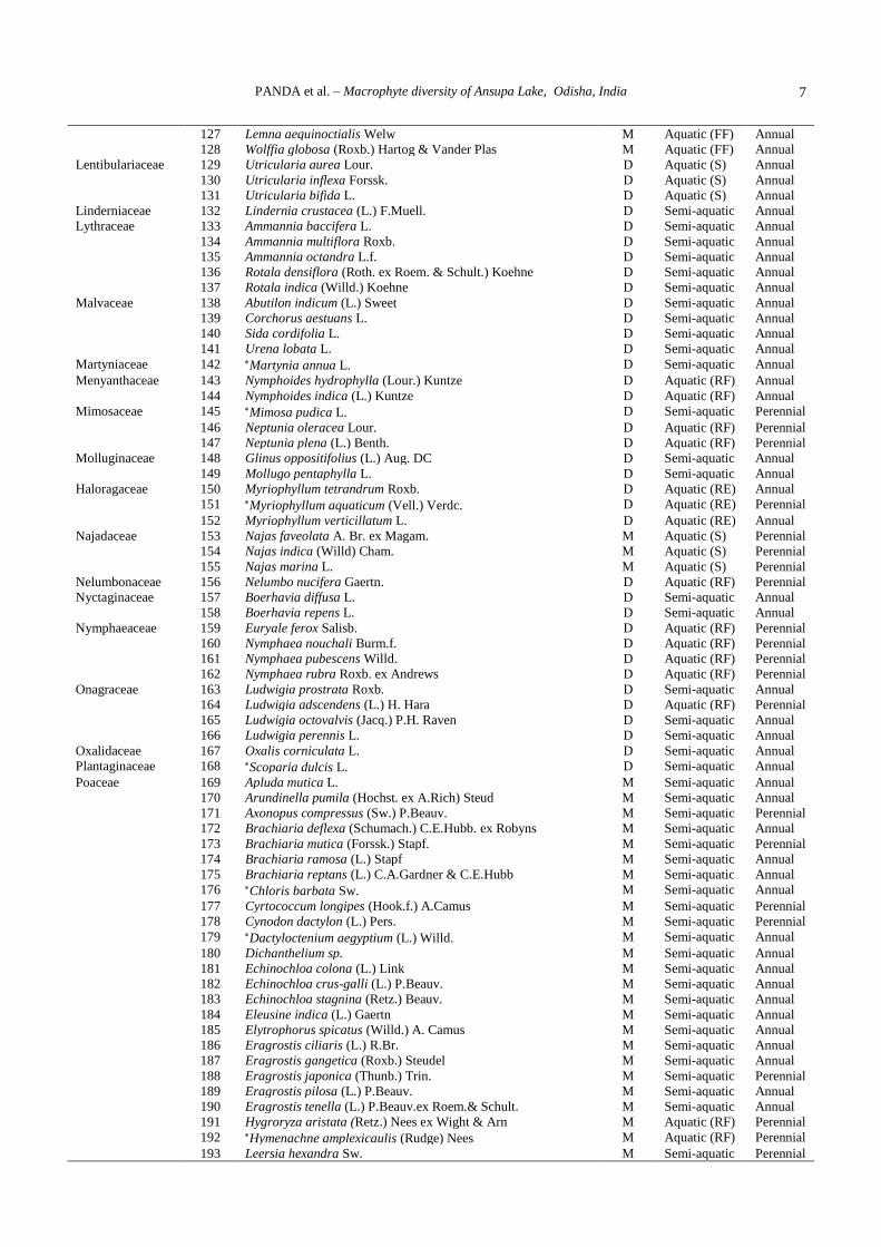
Table 1. List of Angiospermic macrophyte recorded from Ansupa Lake, Odisha, India
Plant family Si. No. Plant species Plant
group
Macrophyte
type
Life
form
Acanthaceae 1 Andrographis paniculata (Burm.f.) Wall. ex Nees D Semi-aquatic Annual
2 Hygrophila auriculata (Schum) Heine D Semi-aquatic Annual
3 Hygrophila schulli (Buch.-Ham.) M.R.Almeida & S.M. Almeida D Semi-aquatic Annual
4 Justicia diffusa Willd D Semi-aquatic Annual
5 Ruellia tuberosa L. D Semi-aquatic Annual
Aizoaceae 6 Trianthema portulacastrum L. D Semi-aquatic Annual
Alismataceae 7 Alisma plantago-aquatica L. M Aquatic (S) Annual
8 Limnophyton obtusifolium (L.) Miq. M Aquatic (S) Annual
9 Sagitaria sagittifolia L. M Aquatic (S) Annual
10 Sagittaria guayanensis var. lappula D. Don M Aquatic (S) Annual
11 Sagitaria trifolia L. M Aquatic (S) Annual
Amaranthaceae 12 Achyranthes aspera L. D Semi-aquatic Annual
13 Aerva lanata (L.) Juss. ex Schult. D Semi-aquatic Annual
14 Alternanthera paronychioides A. St-Hil. D Semi-aquatic Annual
15 Alternanthera philoxeroides (Mart.) Griseb. D Semi-aquatic Annual
16 Alternanthera sessilis (L.) DC. D Semi-aquatic Annual
17 Amaranthus spinosus L. D Semi-aquatic Annual
18 Amaranthus viridis L. D Semi-aquatic Annual
19 Celosia argentea L. D Semi-aquatic Annual
20 Gomphrena celosioides Mart. D Semi-aquatic Annual
Amaryllidaceae 21 Crinum latifolium L. M Aquatic (S) Annual
22 Crinum viviparum (Lam.) R.Ansari & V.J.Nair M Aquatic (RF) Annual
Apiaceae 23 Centella asiatica (L.) Urb. D Semi-aquatic Perennial
24 Hydrocotyle modesta Cham. & Schltdl. D Semi-aquatic Perennial
Aponogetonaceae 25 Aponogeton natans (L.) Engl. & Krause M Aquatic (S) Annual
Araceae
26 Alocasia indica (Roxb.) Schott M Semi-aquatic Perennial
27 Colocasia esculenta (L.) Schott M Semi-aquatic Perennial
28 Pistia stratiotes L. M Aquatic (FF) Perennial
Asteraceae 29 Ageratum conyzoides L. D Semi-aquatic Perennial
30 Blumea lacera (Burm.f.) DC. D Semi-aquatic Annual
31 Caesulia axillaris Roxb. D Semi-aquatic Annual
32 Chromolaena odorata (L.) King & H.E. Robins. D Semi-aquatic Perennial
33 Cyanthillium cinereum (L.) H. Rob D Semi-aquatic Annual
34 Eclipta alba (L.) D Semi-aquatic Annual
35 Eclipta prostrata (L.) L. D Semi-aquatic Annual
36 Enydra fluctuans Lour. D Aquatic (S) Annual
37 Emilia sonchifolia (L.) DC D Semi-aquatic Annual
38 Gnaphalium polycaulon Pers. D Semi-aquatic Annual
39 Grangea maderaspatana L. D Semi-aquatic Annual
40 Mikania cordata (Burm.f.) Robinson D Semi-aquatic Annual
41 Sphaeranthus indicus L. D Semi-aquatic Annual
42 Spilanthes paniculata Wall. Ex DC. D Semi-aquatic Annual
43 Synedrella nodiflora (L.) Gaertn. D Semi-aquatic Annual
44 Xanthium strumarium L. D Semi-aquatic Annual
Boraginaceae 45 Coldenia procumbens L. D Semi-aquatic Annual
46 Heliotropium indicum L. D Semi-aquatic Annual
Capparaceae 47 Cleome monophylla L. D Semi-aquatic Annual
48 Cleome viscosa L. D Semi-aquatic Annual
Cariophyaceae 49 Polycarpon prostratum (Forssk.) Asc. & Sch. D Semi-aquatic Annual
Ceratophyllaceae 50 Ceratophyllum demersum L. D Aquatic (S) Perennial
Colchicaceae 51 Gloriosa superba L. M Semi-aquatic Perennial
Commelinaceae 52 Commelina benghalensis L. M Semi-aquatic Perennial
53 Commelina erecta L. M Semi-aquatic Perennial
54 Commelina longifolia Lam. M Semi-aquatic Perennial
55 Cyanotis axillaris (L.) D.Don ex Sweet M Semi-aquatic Perennial
56 Evolvulus nummularius (L.) L. M Semi-aquatic Perennial
57 Murdannia nudiflora (Linn.) Brenan. M Semi-aquatic Annual
58 Murdannia spirata (L.) Bruckn. M Semi-aquatic Annual
Convolvulaceae 59 Ipomoea aquatica Forssk. D Aquatic (RF) Perennial
60 Ipomoea carnea Jacq. ssp. Fistulosa (Mart. ex Choisy) Austin D Semi-aquatic Perennial

BONOROWO WETLANDS 8 (1): 1-12, June 2018
6
61 Ipomoea pes-tigridis L. D Semi-aquatic Perennial
62 Merremia tridentata (L.) Hall. f. D Semi-aquatic Perennial
Costaceae 63 Costus speciosus (J.Koenig) Sm. M Semi-aquatic Perennial
Crassulaceae 64 Bryophyllum calycinum Salisb. D Semi-aquatic Perennial
Cucurbitaceae 65 Mukia maderaspatana (L.) M. Roem. D Semi-aquatic Annual
66 Cucumis melo L. D Semi-aquatic Annual
Cyperaceae 67 Cyperus alopecuroides Rottb. M Semi-aquatic Annual
68 Cyperus brevifolius (Rottb.) Hassk. M Semi-aquatic Perennial
69 Cyperus cephalotes Vahl M Semi-aquatic Perennial
70 Cyperus compressus L. M Semi-aquatic Annual
71 Cyperus corymbosus Rottb. M Semi-aquatic Perennial
72 Cyperus difformis L. M Semi-aquatic Annual
73 Cyperus haspan L M Semi-aquatic Annual
74 Cyperus imbricatus Retz. M Semi-aquatic Perennial
75 Cyperus iria L. M Semi-aquatic Annual
76 Cyperus platystylis R. Br. M Semi-aquatic Perennial
77 Cyperus polystachyos Rottb. M Semi-aquatic Perennial
78 Cyperus rotundus L. M Semi-aquatic Perennial
79 Cyperus strigosus L. M Semi-aquatic Perennial
80 Eleocharis acutangula (Roxb.) schutt. M Aquatic (RE) Perennial
81 Echinochloa crus-galli (L.) P. Beauv. M Semi-aquatic Annual
82 Eleocharis dulcis (Burm.f.) Trin. ex Henschel M Semi-aquatic Perennial
83 Fimbristylis dipsacea (Rottb.) C.B. Clarke M Semi-aquatic Annual
84 Fimbristylis ferruginea (L) Vahl. M Semi-aquatic Perennial
85 Fimbristylis littoralis Gaudich. M Semi-aquatic Annual
86 Fimbristylis miliacea (L.) Vahl M Semi-aquatic Annual
87 Fuirena ciliaris (L.) Roxb. M Semi-aquatic Annual
88 Kyllinga tenuifolia Steud. M Semi-aquatic Annual
89 Lipocarpha chinensis (Osbeck) J.Kern. M Semi-aquatic Annual
90 Cyperous compactus Retz. M Semi-aquatic Annual
91 Pycreus pumilus (L.) Nees M Semi-aquatic Annual
92 Schoenoplectus articulatus (L.) Palla M Semi-aquatic Annual
93 Schoenoplectus grossus (L.f.) Palla M Semi-aquatic Perennial
94 Schoenoplectiella supina (L.) Lye M Semi-aquatic Annual
Elatinaceae 95 Bergia ammannioides Roxb. ex Roth D Semi-aquatic Annual
96 Bergia capensis L. D Semi-aquatic Perennial
Eriocaulaceae 97 Eriocaulon quinquangulare L. M Semi-aquatic Perennial
Euphorbiaceae 98 Acalypha indica L. D Semi-aquatic Annual
99 Croton bonplandianus (Baill.) Kuntze D Semi-aquatic Annual
100 Euphorbia hirta L. D Semi-aquatic Annual
101 Euphorbia prostrata Aiton. D Semi-aquatic Annual
102 Jatropha gossypiifolia L. D Semi-aquatic Perennial
103 Phyllanthus tenellus Roxb. D Semi-aquatic Perennial
104 Ricinus communis L. D Semi-aquatic Perennial
Fabaceae 105 Aeschynomene aspera L. D Semi-aquatic Annual
106 Aeschynomene indica L. D Semi-aquatic Annual
107 Alysicarpus vaginalis (L.) DC. D Semi-aquatic Annual
108 Cassia tora L. D Semi-aquatic Annual
109 Crotalaria pallida Aiton D Semi-aquatic Perennial
110 Crotalaria quinquefolia L. D Semi-aquatic Perennial
111 Zornia diphylla (L.) Pers. D Semi-aquatic Annual
112 Senna obtusifolia (L.) H.S.Irwin. & Barneby D Semi-aquatic Annual
113 Senna occidentalis (L.) Link D Semi-aquatic Annual
114 Sesbania bispinosa (Jacq.) W.F. Wt. D Semi-aquatic Annual
Gentianaceae 115 Hoppea dichotoma Willd. D Semi-aquatic Annual
Hydrocharitaceae 116 Blyxa echinosperma (Clarke) Hook.f. M Aquatic (S) Annual
117 Hydrilla verticillata (L.f.) Royle M Aquatic (S) Perennial
118 Nechamandra alternifolia (Roxb. ex Wight) Thw. M Aquatic (S) Perennial
119 Ottelia alismoides (L.) Pers. M Aquatic (S) Perennial
120 Vallisneria natans (Lour.) H. Hara M Aquatic (S) Annual
Hydrophyllaceae 121 Hydrolea zeylanica (L.) Vahl. D Aquatic (RE) Annual
Lamiaceae 122 Anisomeles indica (L.) O. Kuntze. D Semi-aquatic Perennial
123 Leucas aspera (Willd.) Link D Semi-aquatic Annual
124 Pogostemon quadrifolius (Benth.) F. Muell. D Semi-aquatic Annual
Lemnaceae 125 Spirodela polyrrhiza (L.) Schleid. M Aquatic (FF) Perennial
126 Lemna gibba L. M Aquatic (FF) Annual
PANDA et al. – Macrophyte diversity of Ansupa Lake, Odisha, India
7
127 Lemna aequinoctialis Welw M Aquatic (FF) Annual
128 Wolffia globosa (Roxb.) Hartog & Vander Plas M Aquatic (FF) Annual
Lentibulariaceae 129 Utricularia aurea Lour. D Aquatic (S) Annual
130 Utricularia inflexa Forssk. D Aquatic (S) Annual
131 Utricularia bifida L. D Aquatic (S) Annual
Linderniaceae 132 Lindernia crustacea (L.) F.Muell. D Semi-aquatic Annual
Lythraceae 133 Ammannia baccifera L. D Semi-aquatic Annual
134 Ammannia multiflora Roxb. D Semi-aquatic Annual
135 Ammannia octandra L.f. D Semi-aquatic Annual
136 Rotala densiflora (Roth. ex Roem. & Schult.) Koehne D Semi-aquatic Annual
137 Rotala indica (Willd.) Koehne D Semi-aquatic Annual
Malvaceae 138 Abutilon indicum (L.) Sweet D Semi-aquatic Annual
139 Corchorus aestuans L. D Semi-aquatic Annual
140 Sida cordifolia L. D Semi-aquatic Annual
141 Urena lobata L. D Semi-aquatic Annual
Martyniaceae 142 Martynia annua L. D Semi-aquatic Annual
Menyanthaceae 143 Nymphoides hydrophylla (Lour.) Kuntze D Aquatic (RF) Annual
144 Nymphoides indica (L.) Kuntze D Aquatic (RF) Annual
Mimosaceae 145 Mimosa pudica L. D Semi-aquatic Perennial
146 Neptunia oleracea Lour. D Aquatic (RF) Perennial
147 Neptunia plena (L.) Benth. D Aquatic (RF) Perennial
Molluginaceae 148 Glinus oppositifolius (L.) Aug. DC D Semi-aquatic Annual
149 Mollugo pentaphylla L. D Semi-aquatic Annual
Haloragaceae 150 Myriophyllum tetrandrum Roxb. D Aquatic (RE) Annual
151 Myriophyllum aquaticum (Vell.) Verdc. D Aquatic (RE) Perennial
152 Myriophyllum verticillatum L. D Aquatic (RE) Annual
Najadaceae 153 Najas faveolata A. Br. ex Magam. M Aquatic (S) Perennial
154 Najas indica (Willd) Cham. M Aquatic (S) Perennial
155 Najas marina L. M Aquatic (S) Perennial
Nelumbonaceae 156 Nelumbo nucifera Gaertn. D Aquatic (RF) Perennial
Nyctaginaceae 157 Boerhavia diffusa L. D Semi-aquatic Annual
158 Boerhavia repens L. D Semi-aquatic Annual
Nymphaeaceae 159 Euryale ferox Salisb. D Aquatic (RF) Perennial
160 Nymphaea nouchali Burm.f. D Aquatic (RF) Perennial
161 Nymphaea pubescens Willd. D Aquatic (RF) Perennial
162 Nymphaea rubra Roxb. ex Andrews D Aquatic (RF) Perennial
Onagraceae 163 Ludwigia prostrata Roxb. D Semi-aquatic Annual
164 Ludwigia adscendens (L.) H. Hara D Aquatic (RF) Perennial
165 Ludwigia octovalvis (Jacq.) P.H. Raven D Semi-aquatic Annual
166 Ludwigia perennis L. D Semi-aquatic Annual
Oxalidaceae 167 Oxalis corniculata L. D Semi-aquatic Annual
Plantaginaceae 168 Scoparia dulcis L. D Semi-aquatic Annual
Poaceae 169 Apluda mutica L. M Semi-aquatic Annual
170 Arundinella pumila (Hochst. ex A.Rich) Steud M Semi-aquatic Annual
171 Axonopus compressus (Sw.) P.Beauv. M Semi-aquatic Perennial
172 Brachiaria deflexa (Schumach.) C.E.Hubb. ex Robyns M Semi-aquatic Annual
173 Brachiaria mutica (Forssk.) Stapf. M Semi-aquatic Perennial
174 Brachiaria ramosa (L.) Stapf M Semi-aquatic Annual
175 Brachiaria reptans (L.) C.A.Gardner & C.E.Hubb M Semi-aquatic Annual
176 Chloris barbata Sw. M Semi-aquatic Annual
177 Cyrtococcum longipes (Hook.f.) A.Camus M Semi-aquatic Perennial
178 Cynodon dactylon (L.) Pers. M Semi-aquatic Perennial
179 Dactyloctenium aegyptium (L.) Willd. M Semi-aquatic Annual
180 Dichanthelium sp. M Semi-aquatic Annual
181 Echinochloa colona (L.) Link M Semi-aquatic Annual
182 Echinochloa crus-galli (L.) P.Beauv. M Semi-aquatic Annual
183 Echinochloa stagnina (Retz.) Beauv. M Semi-aquatic Annual
184 Eleusine indica (L.) Gaertn M Semi-aquatic Annual
185 Elytrophorus spicatus (Willd.) A. Camus M Semi-aquatic Annual
186 Eragrostis ciliaris (L.) R.Br. M Semi-aquatic Annual
187 Eragrostis gangetica (Roxb.) Steudel M Semi-aquatic Annual
188 Eragrostis japonica (Thunb.) Trin. M Semi-aquatic Perennial
189 Eragrostis pilosa (L.) P.Beauv. M Semi-aquatic Annual
190 Eragrostis tenella (L.) P.Beauv.ex Roem.& Schult. M Semi-aquatic Annual
191 Hygroryza aristata (Retz.) Nees ex Wight & Arn M Aquatic (RF) Perennial
192 Hymenachne amplexicaulis (Rudge) Nees M Aquatic (RF) Perennial
193 Leersia hexandra Sw. M Semi-aquatic Perennial

BONOROWO WETLANDS 8 (1): 1-12, June 2018
8
194 Oryza rufipogon Griff. M Semi-aquatic Perennial
195 Panicum sumatrense Roth M Semi-aquatic Perennial
196 Paspalum dilatatum Poir M Semi-aquatic Annual
197 Paspalum distichum L. M Semi-aquatic Perennial
198 Paspalum vaginatum Sw. M Semi-aquatic Annual
199 Setaria pumila (Poir.) Roem. & Schult. M Semi-aquatic Annual
200 Saccharum spontaneum L M Semi-aquatic Perennial
201 Setaria glauca (L.) Beauv. M Semi-aquatic Annual
202 Sporobolus coromandelianus (Retzi.) Kunth M Semi-aquatic Annual
Papilionaceae 203 Sesbania bispinosa (Jacq.) W.Wight. D Semi-aquatic Annual
Polygonaceae 204 Persicaria glabrum (Willd.) M.Gomez D Semi-aquatic Perennial
205 Polygonum barbatum L. D Semi-aquatic Perennial
206 Polygonum plebeium R. Br. D Semi-aquatic Annual
207 Rumex maritimus L. D Semi-aquatic Annual
Pontederiaceae 208 Eichhornia crassipes (Mart.) Solm-Laub. M Aquatic (RF) Perennial
209 Monochoria hastata (L.) Solm. M Aquatic (RF) Perennial
210 Monochoria vaginalis (Burm f.) Presl. M Aquatic (RE) Perennial
Portulacaceae 211 Portulaca oleracea L. D Semi-aquatic Annual
Potamogetonaceae
212 Potamogeton nodosus Poir. M Aquatic (S) Annual
213 Stuckenia pectinata (L.) Börner M Aquatic (S) Perennial
Rubiaceae 214 Dentella repens (L.) Forst. et Forst. D Semi-aquatic Annual
215 Oldenlandia diffusa (Willd.) Roxb. D Semi-aquatic Annual
216 Mitracarpus hirtus (L.) DC. D Semi-aquatic Annual
217 Oldenlandia corymbosa L. D Semi-aquatic Annual
Scrophulariaceae
218 Bacopa monnieri (L.) Pennell. D Semi-aquatic Annual
219 Dopatrium junceum (Roxb.) Buch-Ham. ex Benth. D Aquatic (RE) Annual
220 Limnophila aquatica (Roxb.) Alston D Aquatic (RE) Annual
221 Limnophila heterophylla (Roxb.) Benth. D Aquatic (RE) Annual
222 Limnophila indica (L.) Druce D Aquatic (RE) Annual
223 Limnophila sessiliflora (Vahl) Blume D Aquatic (RE) Annual
224 Lindernia anagallis (Burm.f.) Pennel D Semi-aquatic Annual
225 Lindernia antipoda (L.) Alston D Semi-aquatic Annual
226 Lindernia parviflora (Roxb.) Haines D Semi-aquatic Annual
227 Mecardonia procumbens (Mills.) Small D Semi-aquatic Annual
228 Scoparia dulcis L. D Semi-aquatic Annual
229 Verbascum chinense (L.) Santapau D Semi-aquatic Annual
Solanaceae 230 Physalis minima L. D Semi-aquatic Annual
Sphenocleaceae 231 Sphenoclea zeylanica Gaertn. D Semi-aquatic Annual
Sterculiaceae 232 Melochia corchorifolia L. D Semi-aquatic Annual
Trapaceae 233 Trapa natans L. var. bispinosa (Roxb.) Makino D Aquatic (RF) Perennial
Typhaceae 234 Typha angustata Bory & Chaub. M Aquatic (RE) Perennial
Verbenaceae 235 Lantana camara L. D Semi-aquatic Perennial
236 Lippia javanica (Burm.f.) Spreng. D Semi-aquatic Perennial
237 Phyla nodiflora (L.) Greene D Semi-aquatic Annual
Violaceae 238 Hybanthus enneaspermus (L.) F.Muell. D Semi-aquatic Annual
Note: D= Dicot, M= Monocot, S= Submerged, FF= Free floating, RF= Rooted floating, RE= Rooted erect, =Exotic or non native
species (Un-marked species are native or indigenous to India)
Table 2. List of Non-flowering (Pteridophyte) macrophytes of Ansupa Lake (Odisha), India
Family S. No. Plant species Habitat group Life form
Marsileaceae 1 Marsilea minuta L. Aquatic (RF) Perennial
2 Marsilea quadrifolia L. Aquatic (RF) Perennial
Salviniaceae 3 Azolla microphylla Kaulf. Aquatic (FF) Annual
4 Azolla pinnata R.Br. Aquatic (FF) Perennial
5 Salvinia minima Baker Aquatic (FF) Perennial
6 Salvinia molesta D.S. Mitch Aquatic (FF) Perennial
Note: RF=Rooted floating, FF=Free floating, = Exotic or non native species (Un-marked species are native or indigenous to India)

PANDA et al. – Macrophyte diversity of Ansupa Lake, Odisha, India
9
Table 3. Quantitave status of important macrophytes of Ansupa Lake, Odisha, India
Macrophyte species Total count
Total plots where recorded
Frequency Abundance Abundance/ frequency
(A/F)
Eichhornia crassipes (Mart.) Solm-Laub. 31 4 16 7.75 0.484 Ipomoea aquatica Forssk. 17 3 12 5.67 0.472 Cyperus strigosus L. 14 2 8 7.0 0.875 Cyperus iria L. 60 1 4 60.0 15.00 Cyperus rotundus L. 20 1 4 20.0 5.00 Ludwigia adscendens (L.) H. Hara 13 2 8 6.5 0.813 Ludwigia perennis L. 20 3 12 6.67 0.556 Alternanthera philoxeroides (Mart.) Griseb. 25 1 4 25.0 6.250 Salvinia molesta D.S. Mitch 37 3 12 12.33 1.028 Salvinia minima Baker 6 1 4 6.0 1.500 Cyperus compressus L. 62 2 8 31.0 3.875 Kyllinga tenuifolia Steud. 2 1 4 2.0 0.500 Hydrilla verticillata (L.f.) Royle 1240 12 48 103.33 2.153 Ceratophyllum demersum L. 4060 21 84 193.33 2.302 Najas faveolata A. Br. ex Magam. 335 9 36 37.22 1.034 Nymphaea pubescens Willd. 6 4 16 1.5 0.094 Trapa natans L. var. bispinosa (Roxb.) Makino 8 1 4 8.0 2.00 Nelumbo nucifera Gaertn. 57 16 64 3.56 0.056 Pistia stratiotes L. 11 3 12 3.67 0.306 Spirodela polyrrhiza (L.) Schleid. 54 4 16 13.5 0.844 Utricularia sp. 171 4 16 42.75 2.672 Lemna gibba L. 78 7 28 11.14 0.398 Azolla pinnata R Br. 29 5 20 5.8 0.290 Polygonum barbatum L. 38 1 4 38.0 9.500 Marsilea quadrifolia L. 20 3 12 6.67 0.556 Aponogeton natans (L.) Engl. & Krause 5 1 4 5.0 1.250 Hygroryza aristata (Retz.) Nees ex Wight & Arn 7 2 8 3.5 0.438 Lindernia parviflora (Roxb.) Haines 10 2 8 5.0 0.625
A B
C D
Plate 1. Some taxonomically important taxa from Ansupa Lake, Odisha, India. Note: A. Oryza rufipogon, B. Hygroryza aristata, C. Ottelia alismoides, D. Gloriosa superba

BONOROWO WETLANDS 8 (1): 1-12, June 2018
10
A B
C D
E F
G H
Plate 2. Invasive weed species of Ansupa Lake, Odisha, India. Note: A-B. Eichhornia crassipes, C-D. Nelumbo nucifera, E. Salvinia
molesta, F. Ceratophyllum demersum, G. Najas indica, H. Hymenachne amplexicaulis

PANDA et al. – Macrophyte diversity of Ansupa Lake, Odisha, India
11
Besides being having these troublesome weeds, the lake
also hosts many macrophytes that are used as food, fodder
or medicine by the local households. Control of invasion
and their management is a tedious and need multiple
strategies. Management of this invasive grass must include
a combination of strategies such as winter burning,
herbicide application and hydroperiod control. The floating
rotted macrophyte Euryale ferox Salisb., once occurred in
the lake (recorded in October 2014) is now extinct from the
lake. Implementation of physical (mechanical) methods
and dredging to required depth will reduce current infested
weeds and further regular monitoring, participation of both
Governments agency and local community thought to
restore a long term functioning of the lake.
General comments
Aquatic macrophytes are indispensable constituent of
any wetland. They provide habitat to various aquatic fauna,
act as primary producers, oxygenate water, maintain water
quality, do nutrient cycling, stabilize shoreline of lakes,
provide substrate for growth of algae, provide shelter to
benthic fauna and breeding ground for fishes, check inflow
of silt, reduce nutrient load by self utilizing and minimize
development of algal blooms (Naskar 1990; Bornette and
Puijalon 2009; Ansari et al. 2017). But, sometimes
environments enforce and help for invasion of exotic weeds
in aquatic ecosystems which negatively affect the entire
ecosystem. These plants compete with native species and
many times facilitate for loss or extinction of less
aggressive and indigenous species (Stallings et al. 2015).In
many instances they affect negatively to human activities
(e.g. fishing, swimming, navigation and irrigation) and
degrade the physical, chemical or biological aspects (Basak
et al. 2015). In India, about 140 aquatic plants have been
reported as attained the status of aquatic weeds (Naskar
1990, Gupta 2012) and many of them found in Ansupa
Lake. The wetlands in India are also gradually shrinking
and under severe anthropogenic pressure (Pattanaik et al.
2008; Udayakumar and Ajithadoss 2010). Regular physical
visits, application of geospatial remote sensing techniques,
monitoring of change in floristic composition, maintaining
required depth, reducing fertilizer use in agriculture in
nearby cultivation lands, creation of green coverage in
surrounding barren lands can save native biota from alien
species to invade many aquatic ecosystems.
ACKNOWLEDGEMENTS
Authors are thank full to Ministry of Environment,
Forest and Climate Change for providing financial
assistance for Conservation and Management of Ansupa
Lake, Odisha, India for the year 2016-2017 under the
National Plan for Conservation of Aquatic Eco-systems
(NPCA).
REFERENCES
Ansari AA, Saggu S, Al-Ghanim SM, Abbas ZK, Gill SS, Khan FA, Dar
MI, Naikoo MI, Khan AA. 2017. Aquatic plant biodiversity: A
biological Indicator for the Monitoring and Assessment of Water Quality. In: Ansari AA, Gill SS, Abbas ZK, Naeem M (eds). Plant
Biodiversity: Monitoring, Assessment and Conservation. CAB
International, Wallingford. Basak SK, Ali MM, Islam MS, Shaha PR. 2015. Aquatic weeds of Haor
area in Kishoregonj district, Bangladesh: Availability, Threats and
Management Approaches. Intl J Fish Aquat Stud 2 (6): 151-156. Bornette G, Puijalon S. 2009. Macrophytes: Ecology of Aquatic Plants. In
Encyclopedia of Life Sciences (ELS). John Wiley & Sons, Ltd., Chichester, UK.
Brundu G. 2015. Plant invaders in European and Mediterranean inland
waters: profiles, distribution, and threats. Hydrobiologia 746: 61-79. Byers EJ, Cuddington K, Jones CG, Talley TS, Hastings A, Lambrinos
JG, Crooks JA, Wilson WG. 2006. Using ecosystem engineers to
restore ecological systems. Trends Ecol Evol 21: 493-500. Calvert G, Liessmann L. 2014. Wetland Plants of the Townsville-
Burdekin Flood Plain. Lower Burdekin Landcare Association Inc.,
Ayr. Campbell S, Higman P, Slaughter B, Schools E. 2010. A field Guide to
Invasive Plants of Aquatic and Wetland Habitats for Michigan.
Michigan State University Extension, East Lansing, MI, USA. Chambers PA, Lacoul P, Murphy KJ, Thomaz SM. 2008. Global diversity
of aquatic macrophytes in freshwater. Hydrobiologia 595: 9-26.
Chamier J, Schachtschneider K, Maitre DC, Ashton PJ, Wilgen BW. 2012. Impacts of invasive alien plants on water quality, with
particular emphasis on South Africa. Water SA 38 (2): 345-356.
Crow GE, Hellquist CB. 2000. Aquatic and Wetland Plants of Northeastern North America. The University of Wisconsin Press,
Madison, WI. Dalu T, Clegg B, Nhiwatiwa T. 2012. Aquatic macrophytes in a tropical
African reservoir: diversity, communities and the impact of reservoir-
level fluctuations. Trans R Soc S A 67 (3): 117-125.
Das CR, Mohanty S. 2008. Integrate Sustainable Environmental
Conservation of Ansupa Lake: A famous water resource of Orissa, India. Special Issue on Dev. in Water Resources & Power Sectors in
Orissa. Water Energ Intl 65 (4): 62-66.
Das NR. 2012. Introduction to Aquatic and Semi-aquatic Plants of India. Kalyani Publishers, Punjab, India.
Dodds WK. 2002. Freshwater Ecology: Concepts and Environmental
Applications. Academic Press, New York. Gerber A, Cilliers CJ, Ginkel C. van, Glen R. 2004. Easy identification of
Aquatic plants: A guide for the identification of water plants in and
around South African impoundments. South Africa Department of Water Affairs, Pretoria.
Ghosh SK. 2005. Illustrated aquatic and wetland plants in harmony with
mankind. Standard Literature, 76, Acharya Jagadish Chandra Bose Road, Kolkata, India.
Gopal B. 1995. Biodiversity in Freshwater Ecosystems Including
Wetlands, Biodiversity and Conservation in India, A Status Report.
Zoological Survey of India, Calcutta.
Gupta OP. 2012. Weedy aquatic plants: Their utility, menace and
management. Agrobios, India. Haines HH. 1921-1925. The Botany of Bihar and Orisha, 6 parts. London,
Botanical Survey of India, Culcutta. Margalef DR. 1958. Information theory in ecology. Year Book of the
Society for General Systems Research 3: 36-71.
Mohanty S, Das CR. 2008. Community Mobilization and Participation in Implementing Integrated Sustainable Conservation of Ansupa Lake, a
Famous Wetland of Orissa. In: Sengupta M, Dalwani R (eds).
Proceedings of Taal 2007: The 12th World Lake Conference 1240-1246.
Naskar KR. 1990. Aquatic & Semi-aquatic plants of the lower Ganga
delta. Daya Publishing House, Delhi. Oyedeji AA, Abowei JFN. 2012. The Classification, Distribution, Control
and Economic Importance of Aquatic Plants. Intl J Fish Aquat Sci 1
(2): 118-128. Panda SP, Sahoo HK, Subudhi HN, Sahu AK, Mishra P. 2016. Eco-
floristic diversity of Ansupa Lake, Odisha (India) with special
reference to aquatic macrophytes. J Biodiv Photon 116: 537-552. Patra S, Patra AK. 2007. Environment impact assessment of a fresh water
ecosystem operating in Ansupa Lake: An urgent need for
BONOROWO WETLANDS 8 (1): 1-12, June 2018
12
development of fishery resources. In: Proc. Nat. Sem. on
Environment pollution and its protection issues in Orissa. Organised
by Department of Zoology G.S.College. Athagarh.1-2 Sept. 95-98. Pattanaik C, Prasad SN, Reddy CS. 2008. Warning bells in Ansupa Lake,
Orissa. Curr Sci 64 (5): 560.
Pielou EC. 1975. Ecological Diversity. John Wiley and Sons, New York. Sarkar SD, Ekka A, Sahoo AK, Rashith CM, Lianthuamluaia,
Roychowdhury A. 2015. Role of floodplain wetlands in supporting
livelihood: A case study of Ansupa Lake in Odisha. J Environ Sci Comput Sci Eng Technol 4 (3): 819-826.
Shah MA, Reshi ZA. 2012. Invasion by alien macrophytes in freshwater
ecosystems of India. In: Bhatt et al. (eds). Invasive Alien Plants: An Ecological Appraisal for the Indian Subcontinent. CAB International,
Wallingford, UK.
Shannon CE, Wiener W. 1963. The Mathematical Theory of Communication. University of Illinois Press, Urbana, USA.
Simpson EH. 1949. Measurement of diversity. Nature 163: 688.
Stallings KD, Seth-Carley D, Richardson RJ. 2015. Management of Aquatic Vegetation in the Southeastern United states. J Integrat Pest
Manag 6 (1): 1-5.
Udayakumar M, Ajithadoss K. 2010. Angiosperms, Hydrophytes of five
ephemeral lakes of Thiruvallur District, Tamil Nadu, India. Chicklist
6 (2): 270-274. Upadhyay VP, Malviya HS, Behura S, Rout DK. 2009. Ecological
methods for biodiversity assessment in EIA. Indian J Environ Ecoplan
16 (1): 157-168. Varshney JG, Sushilkumar, Mishra JS. 2008. Current Status of Aquatic
Weeds and Their Management in India. In: Sengupta M, Dalwani R
(eds). Proceedings of Taal 2007: The 12th World Lake Conference. Jaipur, India, 28 October– 2 November 2007.
Wang H, Wang Q, Bowler PA, Xiong W. 2016. Invasive aquatic plants in
China. Aquat Invas 11 (1): 1-9. Whitford PB. 1949. Distribution of woodland plants in relation to
succession and clonal growth. Ecology 30: 199-208.
Zedler JB, Kercher S. 2004. Causes and consequences of invasive plants in wetlands: opportunities, opportunists, and outcomes. Crit Rev Plant
Sci 23: 431-452.

BONOROWO WETLANDS P-ISSN: 2088-110X Volume 8, Number 1, June 2018 E-ISSN: 2088-2475
Pages: 13-24 DOI: 10.13057/bonorowo/w080102
Assessing the impacts of climate variability and climate change on
biodiversity in Lake Nakuru, Kenya
MBOTE BETH WAMBUI1, ALFRED OPERE1,, JOHN M. GITHAIGA2, FREDRICK K. KARANJA3 1Department of Meteorology , School of Physical Sciences, University of Nairobi. P.O. Box 30197-00100, Nairobi, Kenya. email:
[email protected], [email protected]
2School of Biological Sciences University of Nairobi Nairobi, Kenya 3Department of Meteorology University of Nairobi Nairobi, Kenya
Manuscript received: 7 December 2017. Revision accepted: 15 May 2018.
Abstract. Wambui MB, Opere A, Githaiga MJ, Karanja FK. 2017. Assessing the impacts of climate variability and climate change on
biodiversity in Lake Nakuru, Kenya. Bonorowo Wetlands 1: 13-24. This study evaluates the impacts of the raised water levels and the
flooding of Lake Nakuru and its surrounding areas on biodiversity, specifically, the phytoplankton and lesser flamingo communities,
due to climate change and climate variability. The study was to review and analyze noticed climatic records from 2000 to 2014. Several
methods were used to ascertain the past and current trends of climatic parameters (temperature, rainfall and evaporation), and also the
physicochemical characteristics of Lake Nakuru (conductivity, phytoplankton, lesser flamingos and the lake depth). These included time
series analysis, and trend analysis, so the Pearson’s correlation analysis was used to show a relationship between the alterations in lake
conductivity to alterations in population estimates of the lesser flamingos and the phytoplankton. Data set extracted from the Coupled
Model Intercomparison Project Phase 5 (CMIP5) (IPCC Fifth Assessment Report (AR5) Atlas subset) models were subjected to time
series analysis method where the future climate scenarios of near surface temperature, rainfall and evaporation were plotted for the
period 2017 to 2100 (projection) for RCP2.6 and RCP8.5 relative to the baseline period 1971 to 2000 in Lake Nakuru were analysed.
The results were used to evaluate the impact of climate change on the lesser flamingos and phytoplankton abundance. It was noticed that
there was a raise in the mean annual rainfall during the study period (2009 to 2014) which brought the increment in the lake’s surface
area from a low area of 31.8 km² in January 2010 to a high of 54.7 km² in Sept 2013, indicating an increment of 22.9 km² (71.92%
surface area increment). Mean conductivity of the lake also lessened leading to the loss of phytoplankton on which flamingos feed
making them to migrate. A strong positive correlation between conductivity and the lesser flamingo population was noticed signifying
that low conductivity affects the growth of phytoplankton and since the lesser flamingos depend on the phytoplankton for their feed, this
subsequently revealed that the phytoplankton density could be a notable predictor of the lesser flamingo occurrence in Lake Nakuru.
There was also a strong positive correlation noticed between phytoplankton and the lesser flamingo population which confirms that feed
availability is a key determining factor of the lesser flamingo distribution in the lake. It is projected that there would be an increment in
temperatures, rainfall and evaporation for the period 2017 to 2100 under RCP2.6 and RCP8.5 relative to the baseline period 1971 to
2000 obtained from the Coupled Model Intercomparison Project phase 5 (CMIP5) multi-model ensemble. As a result, it is expected that
the lake will further increment in surface area and depth by the year 2100 due to increased rainfall thereby affecting the populations of
the lesser flamingos and phytoplankton, as the physicochemical factors of the lake will alter as well during the projected period.
Keywords: Biodiversity, climate change, Lake Nakuru, Kenya
INTRODUCTION
Africa has been known as one of the most easily
damaged regions in the world regarding climate change,
according to the Fourth Assessment report from the
Intergovernmental Panel on Climate Change (IPCC 2007).
A report stated that there are some areas in Africa which
evidently are highly vulnerable to climate variability and
change. Increased changes and variability of different
climatic factors have been forecasted by Kenya’s current
climate predictions. Severe challenges to sustainable
development are being propounded by climate change in
Kenya, as it’s possibly a major environmental challenge of
our time (Mutai et al. 2010). Focusing on effects of climate
change on water resources, coastal zones, ecosystems,
health, industrial activity, food and human settlements,
propounds chances for improved livelihoods, business and
innovation.
Various patterns of rainfall and rising temperatures
have also worsened the problem of wetlands drying out,
thereby threatening water availability leading to lessened
agricultural production and thus accruing food insecurity
due to lessening yields in crop. Various patterns of rainfall
have posed threats to the renowned wildlife safaris in
Kenya, and especially to one of the Seven Wonders of the
World: The Mara River migration of wildebeests, which is
common with tourists around the world (Climate Action
Network 2009). Intermittent patterns of rain affect the
wildebeests as their migration is influenced by the smell of
rain, since the pattern of migration is usually timed to show
a relationship between the growth of grass and annual
rainfall patterns in the North. Drawing closer to March,
which is characterized by a season of short dryness, the
wildebeests begin migrating from Serengeti as the grass
starts drying out towards the western Serengeti woodlands.
By end of June when the long rains commence to decline in

BONOROWO WETLANDS 7 (2): 13-24, June 2018
14
Kenya, the arrival of wildebeest from the Western
Serengeti is noticed in the Maasai Mara Game Reserve.
Scarce feeding vegetation and the drying-up of rivers,
owing to unpredictable climate, has caused huge losses in
wildlife numbers (Climate Action Network 2009).
There is an extensive variety of wildlife and ecosystems
in Kenya, populating in air, water and land. Biodiversity
assets known in Kenya include 7,000 plant species, 315
mammals, 1,133 birds, 25,000 invertebrates (21,575 of
which are insects), 191 reptiles, 692 marine and brackish
fish, 180 freshwater fish, 88 amphibians and about 2,000
species of fungi and bacteria (NEMA 2009a). Kenya boasts
a large population of mammalian species’ ranking it third
in Africa, with fourteen of these species endemic to the
country (IGAD 2007). Large mammals such as the African
elephant (Loxodonta africana), leopard (Panthera pardus),
black rhino (Diceros bicornis), African lion (Panthera leo)
and buffalo (Syncerus cafer) have made the country
become popular due to their diverse nature (NEMA 2009a).
According to the IUCN Threat Criteria (2008), 146 plant
species of the 7000 found in Kenya have been assessed
with 103 being classified as threatened (vulnerable,
endangered or seriously endangered) (NEMA 2011).
In Kenya, threats to biodiversity have been on the
increment over the past decades due to human-wildlife
conflicts, habitat loss, population increment and
infrastructure development, global climate change,
pollution, biopiracy, poaching and overexploitation,
invasive alien species and biosafety concerns (Government
of Kenya (GoK), National Environment Management
Agency (NEMA 2011). In this regard, safeguarding these
biodiversity will be critical to securing livelihoods resulting
to reduced levels of poverty - reflecting a population of
46.6 percent - suggesting a nine percent alteration if the
social equity scales are to be attained as projected by the
Vision 2030’s social pillar (NEMA 2011).
Provided crucial coping, mitigation and adaptation
approaches are realized, future climate variability and
climate change impacts can be avoided, delayed or
reduced. About US $500 million per year was needed in
Kenya to address the climate change effects by 2012
(Stockholm Environment Institute 2009). US $1-2 billion
per year was the amount this figure was forecasted to raise
to by 2030 (Stockholm Environment Institute 2009). The
collective effect of impacts of climate change will limit the
realization of Vision 2030 targets, unless there is an urgent
institutionalization of effective adaptation and mitigation
mechanisms. As such, in order to tackle climate change, a
range of policy instruments need to be formulated. A
national policy on climate change need to be formulated
and a climate change law further enacted, recognizing that
the National Climate Change Response Strategy (NCCRS)
was finalized in 2010. The country will not only be
economically affected by the impacts of climate change but
also its biodiversity heritage.
The main objective of the research was to evaluate the
impacts of climate variability and climate change on Lake
Nakuru’s biodiversity, Kenya, i.e., (i) to estimate the trends
of past and present climatic records, and especially the
temperature, rainfall and evaporation, of Lake Nakuru
basin in order to understand the causes of increased lake
levels. (ii) to show a relationship between alterations in
lake conductivity to alterations in population estimates of
aquatic species especially the phytoplankton and the lesser
flamingos of Lake Nakuru basin. (iii) Evaluate in light of
future climate projections, especially temperature, rainfall,
and evaporation, the likely impacts of climate change on
Kenya’s biodiversity especially the lesser flamingos and
phytoplankton in Lake Nakuru basin.
MATERIALS AND METHODS
Area of study
The study site was Lake Nakuru. It was chosen because
it is one of the most important habitats for the flamingo
species and also one of the important tourist destinations in
Kenya. Lake Nakuru National Park, Kenya is located
between 0°19'- 0°24' S and 36°04'-36°07 E, approximately
3km South of Nakuru town, Kenya. It lies in a graben
between Lion Hill fracture zone in the east and a series of
east downthrown step-fault scarps leading to the Mau
Escarpment to the west.
Lake Nakuru extends in the N-S direction in the trend
of the axial rift faults as shown by Figure 1. It includes
other chains of alkaline-saline lakes in the eastern arm of
the Rift Valley, Kenya. Existing more than twelve million
years, one of the earth’s spectacular geological formations
was formed by the catchment and its landforms which
included rifts, cliffs, mountains, volcanoes and lakes
(Odada et al. 2006). Progressions of characteristics and
features that describe Lake Nakuru have been influenced
by climate, evolutionary history and Geography. Levels of
productivity and successful establishment of species have
been ascertained by these features which set in motion the
chemistry of the lakes’ water. The ecosystem of the lake is
made unique by the chemistry of the alkaline water which
depends on the larger catchment for sustenance and
independent of its immediate environment for it functions.
White salt filets swirling with dust devils are sometimes
created when there are enormous water body reductions
resulting from alterations in the surface area of the lake.
Data type
Data used in this study included climatic data
comprising of mean annual temperature, mean annual
rainfall mean annual evaporation and the Coupled Model
Intercomparison Project Phase 5 (CMIP5) Representative
Concentration Pathways (RCP2.6 and RCP8.5) near
surface temperature, rainfall and evaporation data. Lake
data comprised of conductivity, lake levels, surface area
and depth. Flamingo data comprised of the lesser flamingo
population. Below is a detailed description of the data types
and their sources.
Procedures
In this section, the methods that were used in the study
for data collection, organization and analysis based on the
specific objectives of the study are propounded.
WAMBUI et al. – Impacts of climate change on biodiversity in Lake Nakuru, Kenya
15
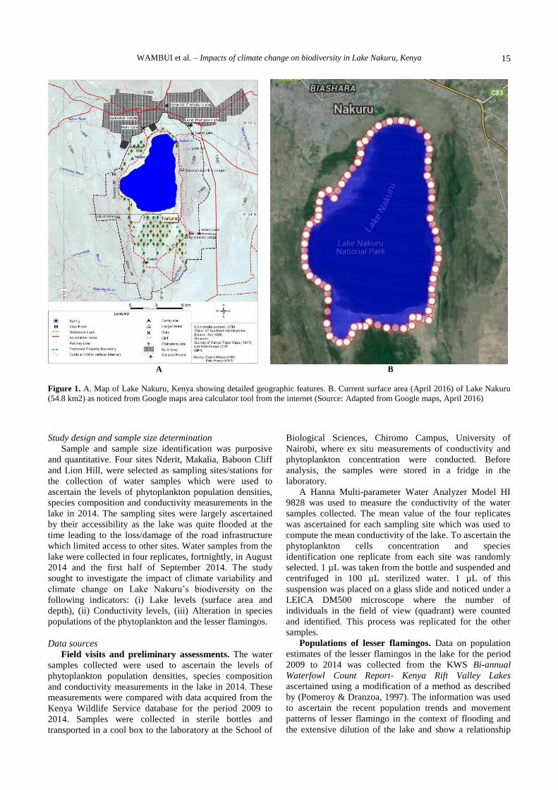
A B
Figure 1. A. Map of Lake Nakuru, Kenya showing detailed geographic features. B. Current surface area (April 2016) of Lake Nakuru
(54.8 km2) as noticed from Google maps area calculator tool from the internet (Source: Adapted from Google maps, April 2016)
Study design and sample size determination
Sample and sample size identification was purposive
and quantitative. Four sites Nderit, Makalia, Baboon Cliff
and Lion Hill, were selected as sampling sites/stations for
the collection of water samples which were used to
ascertain the levels of phytoplankton population densities,
species composition and conductivity measurements in the
lake in 2014. The sampling sites were largely ascertained
by their accessibility as the lake was quite flooded at the
time leading to the loss/damage of the road infrastructure
which limited access to other sites. Water samples from the
lake were collected in four replicates, fortnightly, in August
2014 and the first half of September 2014. The study
sought to investigate the impact of climate variability and
climate change on Lake Nakuru’s biodiversity on the
following indicators: (i) Lake levels (surface area and
depth), (ii) Conductivity levels, (iii) Alteration in species
populations of the phytoplankton and the lesser flamingos.
Data sources
Field visits and preliminary assessments. The water
samples collected were used to ascertain the levels of
phytoplankton population densities, species composition
and conductivity measurements in the lake in 2014. These
measurements were compared with data acquired from the
Kenya Wildlife Service database for the period 2009 to
2014. Samples were collected in sterile bottles and
transported in a cool box to the laboratory at the School of
Biological Sciences, Chiromo Campus, University of
Nairobi, where ex situ measurements of conductivity and
phytoplankton concentration were conducted. Before
analysis, the samples were stored in a fridge in the
laboratory.
A Hanna Multi-parameter Water Analyzer Model HI
9828 was used to measure the conductivity of the water
samples collected. The mean value of the four replicates
was ascertained for each sampling site which was used to
compute the mean conductivity of the lake. To ascertain the
phytoplankton cells concentration and species
identification one replicate from each site was randomly
selected. 1 µL was taken from the bottle and suspended and
centrifuged in 100 µL sterilized water. 1 µL of this
suspension was placed on a glass slide and noticed under a
LEICA DM500 microscope where the number of
individuals in the field of view (quadrant) were counted
and identified. This process was replicated for the other
samples.
Populations of lesser flamingos. Data on population
estimates of the lesser flamingos in the lake for the period
2009 to 2014 was collected from the KWS Bi-annual
Waterfowl Count Report- Kenya Rift Valley Lakes
ascertained using a modification of a method as described
by (Pomeroy & Dranzoa, 1997). The information was used
to ascertain the recent population trends and movement
patterns of lesser flamingo in the context of flooding and
the extensive dilution of the lake and show a relationship

BONOROWO WETLANDS 7 (2): 13-24, June 2018
16
between the alterations in lake conductivity to alterations in
the population estimates of the phytoplankton and lesser
flamingo for the period 2009 to 2014.The data was based
on records of the January water bird counts that are
conducted jointly by the National Museums of Kenya and
Kenya Wildlife Service.
Alterations in the lake levels. Data to ascertain the
alterations in the lake surface area and depth was obtained
from (Onywere et al. 2013) and the Kenya Wildlife Service
records respectively. Documentation of the alterations in
the lake surface area was made using Geographic
Information System (GIS) digital techniques and
information extraction and representation from Landsat
satellite image data for January 2010, May 2013 and
September 2013 and October 2013 (Onywere et al. 2013),
whereas monthly measurements of the depth of the lake
was collected from KWS. This had been ascertained from
the readings of a staff gauge located at the lake centre.
Physicochemical characteristics of water
(phytoplankton concentration and conductivity). The
physicochemical qualities of water (phytoplankton
concentration and conductivity) for the period 2009-2013
were obtained from the Kenya Wildlife Service (KWS)
database. Monthly measurements of conductivity and
concentration of phytoplankton in lake water had been
ascertained based on monthly analysis of water taken from
the lake centre. Conductivity had been ascertained using a
pH meter. The concentration of phytoplankton had been
ascertained using the Sedgewick-Rafter counting chamber
as described by Kimberly (1999).
Noticed climate data. The climatic data (Rainfall,
temperature, evaporation) for the period 2009 to 2014 was
collected from the Kenya Meteorological Department,
based on monthly data from the Nakuru Meteorological
Station - 9036261(0.28oS, 36.1oE), located 3km north of
the lake at the Nakuru Agricultural show grounds.
Climate projection data sets. In this study, the
projected alterations in near surface temperature, rainfall
and evaporation for Lake Nakuru were extracted from the
Coupled Model Intercomparison Project Phase 5 (CMIP5)
multi-model ensemble (IPCC Fifth Assessment Report
(AR5) Atlas subset) models. The output data were
extracted as a relative alteration from 1971 to 2000
(baseline) to, 2017 to 2100 (projection) under two
scenarios, namely, the RCP2.6 and RCP8.5 scenarios
(Taylor et al. 2012). The RCP2.6 and RCP8.5 represent
‘low’ (RCP2.6) and ‘high’ (RCP8.5) scenarios featured by
the radiative forcings of 2.6 and 8.5 Wm−2 by 2100,
respectively. The CO2 equivalent concentrations in the
year 2100 for RCP 2.6 and RCP 8.5 are 490 ppm and 1370
ppm, respectively (Moss et al. 2010). RCP2.6 and RCP8.5
were chosen for this study as RCP2.6 describes an all-out
effort to limit global warming to below 2°C with emissions
lessening sharply after 2020 and zero from 2080 onward,
whereas RCP8.5 describes a business-as-usual scenario
with accruing greenhouse gas emissions over time, leading
to high greenhouse gas concentration levels.
These Representative Concentration Pathways (RCPs)
are among four new GHG concentration developed
scenarios set containing emission, concentration and land-
use trajectories which have been adopted by the IPCC Fifth
Assessment Report (AR5) (Moss et al. 2010; Van Vuuren
et al. 2011; IPCC 2014). They describe possible climate
futures explaining the possible range of forcing values up
to the year 2100, with respect to the situation before
industrialization. RCP2.6 and RCP8.5 were chosen for this
study as they
Data quality control
Data quality control was conductedconducted to ensure
that the data sets were devoid of missing values, consistent,
uniformly entered and arranged to facilitate further
processing. The data was then subjected to various
statistical computations.
Homogeneity test. Most long-term climatological data
records have been affected by a number of non-climatic
factors that make these records unsuitable for comparison
over long time periods and between different stations.
These relate to alterations that can affect instruments, site,
or procedures and methods in the observations and data
processing. These factors are caused by alterations in:
instrumentation, observation practices, location of station,
and formulae used for means calculation, and changing the
environment of the station. While some alterations make
critical discontinuities, others, particularly alterations
around station environment, due for example to,
urbanisation, causes data biases which are gradual leading
to time series biases and studied climate misinterpretations.
In this study, the cumulative mass curve technique
described in the subsection below was used to test for data
homogeneity.
Mass curve. Mass curve analysis entails plotting of
cumulative climatological data records against time to
depict the homogeneity. The patterns of these graphs can
be used to test for the quality of the records. A single
straight line indicates a homogeneous record whereas
heterogeneity tendency is indicated by existence of more
than one line fitted to the graphical plots of the cumulative
data. For the heterogeneous records, correcting the
heterogeneity would be the next step. Double mass curves
are commonly used to adjust heterogeneous records whose
principles are similar to those of mass curves. In this study,
the single mass curve technique was used to test the data
consistence where cumulative rainfall and temperature data
was plotted against time to depict the homogeneity. A
straight line graph depicted homogeneous data.
Time series analysis
Time series is the organization of statistical data in
chronological order; in order with its time of occurrence. In
this study a plotting of the annual means of rainfall,
temperature and evaporation data for the period 2000 to
2014 using graphical method was undertaken. In addition,
annual data means for lake depth, lesser flamingo
population, conductivity, and phytoplankton levels for the
period 2009 to 2014 were also plotted.
In order to ascertain the projected alterations in near
surface temperature, rainfall and evaporation for Lake
Nakuru, data extracted from the Coupled Model
Intercomparison Project Phase 5 (CMIP5) multi-model

WAMBUI et al. – Impacts of climate change on biodiversity in Lake Nakuru, Kenya
17
ensemble (IPCC Fifth Assessment Report (AR5) Atlas
subset) models were plotted using the KNMI (2015) to
analyse the data for the period 2017 to 2100 for RCP2.6
and RCP8.5 relative to the baseline period 1971-2000.
The trend is characterized by the long term movement
that is either represented by a growth or decline in a time
series through a lengthy period of time. The trend in time
series in this study, graphical method was used to
ascertain the past and current trends of climatic
parameters (temperature, rainfall and evaporation), and also
for the physicochemical characteristics of Lake Nakuru
(conductivity, phytoplankton, lesser flamingos and the lake
depth).
Standard error of the mean was used to provide
information about the distribution of the values within the
trends as shown by Equation (1).
……………………………………………… (1)
Where, σM is the standard error of the mean, σ is the
standard deviation of the original distribution and N is the
sample size (the number of counts each mean is based
upon). Specifically in this study, the error bars were fitted
graphically to evaluate whether there was a notable
difference between the data sets. While a larger sample size
suggests a smaller standard error of the mean, overlapping
error bars implies that the difference is usually not notable.
However, when the error bars do not overlap, it suggests
that the difference is notable.
Correlation analysis
The Pearson Correlation coefficient (r), given in
equation (2), was used to quantify the degree of relations
between pairs of study variables. It is used extensively as a
measure of the degree of linear dependence among two
variables. If two variables ‘x’ and ‘y’ are so related, where,
‘x’ is the conductivity of the lake and where, ‘y’ is
represented by either the phytoplankton or the lesser
flamingos, the variables in the magnitude of one variable
tend to be accompanied by variations in the magnitude of
the other variable, they are said to be associated. Therefore,
correlation as a statistical tool helps to ascertain whether or
not two or more variables associate and if they are
associated, the degree and direction of their correlation.
……………. (2)
Where, r is the Pearson correlation coefficient, N is the
sample size, ∑xy is the sum of the products of paired
scores, ∑x is the sum of x scores, ∑y is the sum of y
scores, and ∑x2 is the sum of squared x scores
The student T-test was used to test for the significance
of the correlation coefficient. The computed t-statistic
derived from Equation (3), was compared with the
tabulated t-value of the student t-distribution at the n-2
degrees of freedom and 5% significance level.
……….....................……………... (3)
Where, n represents the length of the data that were
used, n-2 is the degree of the freedom, n-2 is the
computed t-statistic and r is the Pearson correlation
coefficient.
Correlation coefficient was deemed to be notable if the
computed value of t was greater than the tabulated value at
the 5% significance level. This is usually conducted to
ascertain whether the linear relationship in the sample data
is strong enough to use to model the relationship in the
population.
RESULTS AND DISCUSSION
Data quality control
In this section, results of data quality control are
propounded and their suitability for the study established.
Specifically this section propounds results of the
homogeneity test. The Figures 2 and 3 show simple mass
curves for rainfall and temperature respectively. It can be
noticed from Figures 2 and 3 that the rainfall and
temperature data sets were homogeneous, owing to the
resistant straight line plots. It can be noted that generally
the rainfall has been gradually accruing leading to an
increment in the surface runoff, most of which
subsequently ended up in the lake.
Figure 2. Single mass curve, cumulative annual rainfall
Figure 3. Single mass curve, cumulative annual temperature

BONOROWO WETLANDS 7 (2): 13-24, June 2018
18
Past and present climatic record of Lake Nakuru from
2000 to 2014
Trend analysis of climatic data
Trends in rainfall patterns from 2000 to 2014. There
has been marked variability of the mean annual rainfall
patterns of Lake Nakuru basin with major rainfall
intensification in the years 2000 to 2001 and 2009 to 2010,
with the highest (120 mm) being recorded in 2010 (Figure 4).
Trends in temperature patterns from 2000 to 2014.
Mean annual temperatures has been on a lessening trend
during the period 2000 to 2014, with the highest temperatures
being recorded in 2000 (26.6ºC) and in 2009 (27ºC) (Figure
5). Evaporation in the Lake Nakuru basin shows a
declining trend over the study period (Figure 6). However,
the noticed decrement in evaporation from the year 2009 is
consistent with the increment in rainfall noticed in Figure 4
and temperature decrement noticed in Figure 5.
Alterations in the lake levels (depth and surface
area) 2009 to 2014. Time series of Lake Nakuru levels
(depth). Lake Nakuru levels have been rising over the years
2009 to 2014 (Figure 7). As seen in Figure 7, the mean
depth of the lake rapidly increased during the study period
(2009 to 2014). This could have been caused by increased
rainfall during the study period which led to increased
surface runoff and direct rainfall into the lake. The
increased water levels led to the flooding of the lake which
further lowered the conductivity of the lake as more fresh
water was added into it.
Alterations in the lake surface area
Lake Nakuru’s surface area increased from an area of
31.8 km² in January 2010 to a high of 54.7 km² in Sept
2013 (Figure 8 and 9), an increment of 22.9 km² (71.9%).
This led to the submergence of 60% of the transport
infrastructure in Lake Nakuru Nationa Park and the park’s
main gate, during this period, thereby displacing wildlife.
At the highest level, the lake expanded and submerged
areas that have never been recorded in the last 100 years
(Figure 9). The extent of the flooded area and the impacts
are illustrated in the image data and digitized maps shown
in Figure 10.
Conductivity, phytoplankton levels and the lesser
flamingos populations
Conductivity levels
The mean conductivity of Lake Nakuru lessened from
the period 2009 to 2014 (Figure 11).
Figure 4. Mean annual rainfall patterns for the period 2000 to 2014
Figure 5. Mean annual temperatures from the year 2000 to 2014
Figure 6. Mean annual evaporation patterns for the year 2000 to
2014
Figure 7. Alterations in the mean depth of Lake Nakuru from
2009 to 2014
Figure 11. Trend in mean conductivity levels from 2009 to 2014
in Lake Nakuru

WAMBUI et al. – Impacts of climate change on biodiversity in Lake Nakuru, Kenya
19
Figure 8. Alterations in the surface are of Lake Nakuru between January 2010 and 2013 (Source: Onywere et al. 2013)
This coincided with the beginning of the rains from the
year 2010 as shown in Figure 4. The declining conductivity
of the lake could result into loss of phytoplankton
(reduction in food supply) upon which the lesser flamingos
feed. This could eventually lead to the migration of the
lesser flamingos from the lake. This is due to the fact that
as more fresh water was added in to the lake, it lowered the
conductivity of the lake because fresh water has low
conductivity and the increment in water levels dilutes
mineral concentrations.
Phytoplankton levels
The phytoplankton levels in Lake Nakuru were quite
variable for the years 2009 to 2014 as shown by Figure 12.
Notably, however, there was a general reduction in the
phytoplankton levels which coincided with the onset of the
rains from the year 2010 as shown in Figure 4.
Phytoplankton levels lessened from 606 Units/mL in 2010
to 187 Units/mL in 2012. However, there was an increment
in the phytoplankton levels to 321 Units/mL in 2013 which
could have been caused by alterations in phytoplankton
species composition and diversity that in turn affected their
abundance due to alterations in the chemical and physical
properties of the water (Kihwele et al. 2014).
Lesser flamingos population
The number of lesser flamingos drastically lessened
from the beginning of the rains in 2010 (Figure 13) from
41,592 in 2010 to 10,168 in 2011 and further lessened to
110 in 2012. This pattern follows that of lessening
phytoplankton levels shown in Figure 12.
Figure 12. Trend in mean phytoplankton levels in Lake Nakuru
from 2009 to 2014
BONOROWO WETLANDS 7 (2): 13-24, June 2018
20
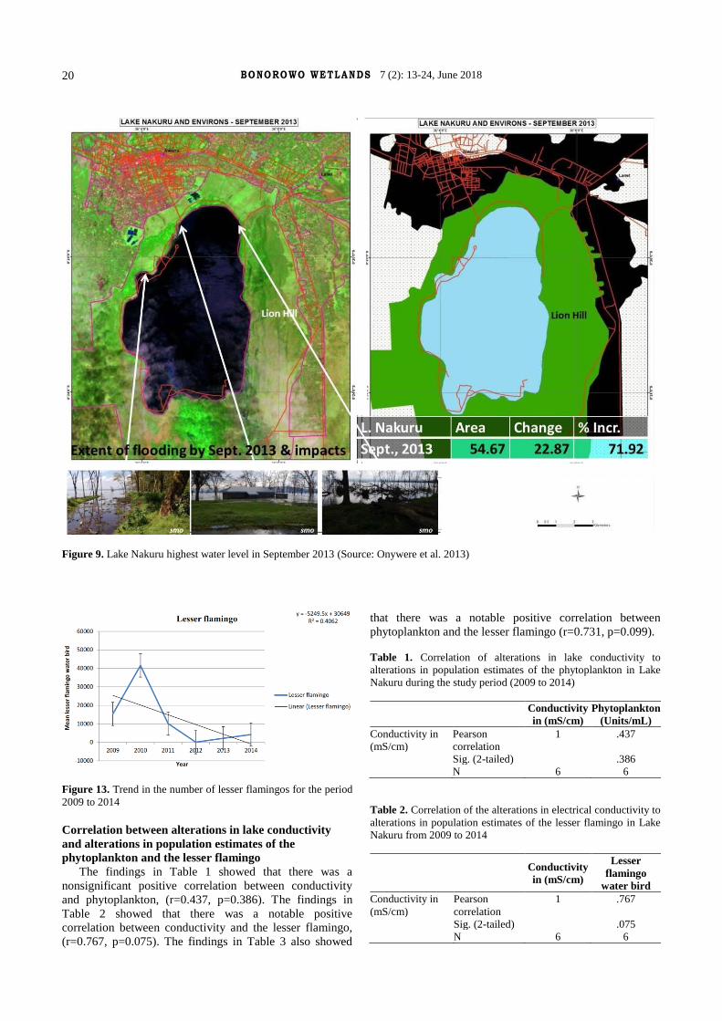
Figure 9. Lake Nakuru highest water level in September 2013 (Source: Onywere et al. 2013)
Figure 13. Trend in the number of lesser flamingos for the period
2009 to 2014
Correlation between alterations in lake conductivity
and alterations in population estimates of the
phytoplankton and the lesser flamingo
The findings in Table 1 showed that there was a
nonsignificant positive correlation between conductivity
and phytoplankton, (r=0.437, p=0.386). The findings in
Table 2 showed that there was a notable positive
correlation between conductivity and the lesser flamingo,
(r=0.767, p=0.075). The findings in Table 3 also showed
that there was a notable positive correlation between
phytoplankton and the lesser flamingo (r=0.731, p=0.099).
Table 1. Correlation of alterations in lake conductivity to
alterations in population estimates of the phytoplankton in Lake
Nakuru during the study period (2009 to 2014)
Conductivity
in (mS/cm)
Phytoplankton
(Units/mL)
Conductivity in
(mS/cm)
Pearson
correlation
1 .437
Sig. (2-tailed) .386
N 6 6
Table 2. Correlation of the alterations in electrical conductivity to
alterations in population estimates of the lesser flamingo in Lake
Nakuru from 2009 to 2014
Conductivity
in (mS/cm)
Lesser
flamingo
water bird
Conductivity in
(mS/cm)
Pearson
correlation
1 .767
Sig. (2-tailed) .075
N 6 6

WAMBUI et al. – Impacts of climate change on biodiversity in Lake Nakuru, Kenya
21
Figure 10. Time series extent of flooding in Lake Nakuru from a low area of 31.8 km² in January 2010 to a high of 54.7 km² in Sept
2013, a total increment of 22.9 km² (71.9%) (Onywere et al. 2013)
Table 3. Correlation of the alterations in the population estimates
of the lesser flamingo in Lake Nakuru to alterations in the
population estimates of the phytoplankton from 2009 to 2014
Lesser flamingo
water bird
Phytoplankton
(units/mL)
Lesser flamingo
water bird
Pearson
correlation
1 .731
Sig. (2-
tailed)
.099
N 6 6
Projections of the climatic data (temperatures,
evaporation and rainfall) for the period 2017-2100
Future climate scenarios of Lake Nakuru comprising
near surface temperature, rainfall and evaporation were
plotted for the period 2017 to 2100 (projection) for RCP2.6
and RCP8.5 relative to the baseline period 1971 to 2000.
The results obtained are sequentially propounded in the
subsections that follow.
Near surface temperature projections
Future alterations in annual temperature for Lake
Nakuru under RCP2.6 and RCP8.5 for the period 2017 to
2100 relative to baseline period 1971 to 2000 are
propounded in Figure 14 and 15 respectively.
Temperature projections indicate an accruing trend with
a 1.2°C increment for the 2071 to 2100 mean alterations for
RCP2.6 (Figure 14) whereas there is a 4.8°C increment for
the 2071 to 2100 mean alterations for RCP8.5 (Figure 15).
The likely causes of the accruing trend of temperature
under both RCP2.6 and RCP8.5 could be due to accruing
levels of greenhouse gas concentrations in the atmosphere
during the projected period. Notably however, the rate of
temperature increment in RCP2.6 is lower than that of
RCP8.5.
Rainfall projections
Future alterations in rainfall for Lake Nakuru under
RCP2.6 and RCP8.5 were plotted for the period 2017 to
2100 relative to baseline period 1971 to 2000 are shown in
Figures 16 and 17 respectively.
The rainfall projection from RCP2.6 and RCP 8.5 show
a 10% and 20 % increment in rainfall for the 2071 to 2100.

BONOROWO WETLANDS 7 (2): 13-24, June 2018
22
Evaporation projections
Future alterations in evaporation for Lake Nakuru under
RCP2.6 and RCP8.5 for the period 2017 to 2100 relative to
baseline period 1971 to 2000 are shown in Figures 18 and
19.
Relative evaporation is projected to raise by 10% and
20% for the 2071 to 2100 mean changes for RCP2.6 and
RCP8.5 respectively.
Figure 14. Near surface temperature projection for RCP2.6 for
the Lake Nakuru area from 2017 to 2100 shows a 1.2°C
increment for the 2071 to 2100 mean alterations
Figure 15. Near surface temperature projection for RCP8.5 for
the Lake Nakuru area from 2017 to 2100 shows a 4.8°C
increment for the 2071 to 2100 mean alterations
Figure 16. Rainfall projections for RCP2.6 for Lake Nakuru
Figure 17. Rainfall projections for RCP8.5 show a 20%
increment in rainfall in Lake Nakuru area for the 2071 to 2100
mean alterations
Figure 18. Relative evaporation alteration for RCP2.6 for the
Lake Nakuru for 2071 to 2100
Figure 19. Relative evaporation alteration for RCP8.5 for Lake
Nakuru
Discussions
As drawn in Figure 4, it can be concluded that rainfall
has increased since 2010 and this may have greatly affected
the accruing water levels in lakes as shown by the images
obtained from (Onywere et al. 2013). Figure 7 also depicts
that the depth of the lake has gradually increased since the
beginning of the rain in 2010. This can be strongly
associated with increased surface runoff and lake
catchment improvements from Njoro, Makalia, Larmudiac
and Enderit Rivers as well as from direct rainfall to lakes.
WAMBUI et al. – Impacts of climate change on biodiversity in Lake Nakuru, Kenya
23
Figures 5 and 6 depict that temperature and evaporation
have been raising from 2007 to 2009, the same period
when there was little/no rain, and drastically lessened from
2009 to 2010, the beginning of the rainy season. According
to Trenberth (2011), an increment in temperature usually
leads to an increment in evaporation and therefore drought.
Heating about 7% per 1 ° C raises the water holding
capacity of the atmosphere. This is noticed in studies with
temperatures and evaporation raising in 2007 to 2009,
which increased the capacity to water retaining of the
atmosphere, and thus the beginning of rain in 2009.
According to the IPCC (2007), climate change is clearly
more and easily accessed by temperature, although
atmospheric moisture changes, atmospheric circulation and
rainfall are also ascertained because the overall climate
system is generally influenced. The capacity to withstand
atmospheric moisture is made increment as temperature
becomes higher at a rate of about 7% per °C (Trenberth et
al., 2003). Collectively, changes in the hydrological cycle
are influenced, in particular, the characteristics of rainfall
(type, intensity, amount, duration, frequency) and extremes
(Trenberth et al., 2003). The increased water vapor
convergence guides to heavier rainfall but a reduction in
duration and/or frequency in the weather system, given that
the total amount changed a little. Therefore, it can be
concluded that a slight increment in temperature induces a
tighter hydrological cycle because the evaporation rate is
also increased which has a direct impact on cloud
formation, since intense rainfall is affected as atmospheric
water containment capacity increases, as noticed in 2010.
Seasonal hydrological budget changes greatly affect
endorheic lakes that may be extreme at a time, resulting in
drastic algal biomass accidents and major changes in
community composition as has been noticed in Lake
Nakuru.
As more water is added to the lake, it liquidized the
mineral concentration thereby lessened the electrical
conductivity of the lake. Fresh water has low conductivity.
According to the study made in Figure 11, the conductivity
level began to decline at 2010, after the start of the rain.
The relationship between lake water conductivity and lake
depth examined in this study reflects the cycle of
concentration and dilution of the lake due to evaporation
during the dry season followed by replenishment from river
in-flow and water run-off during the wet season. These
hydrological cycles have a profound effect on aquatic biota
in the lake (Githaiga, 1997).
The correlation coefficient in Table 1 showed changes
in lake conductivity and corresponding changes in
phytoplankton population estimates. The undistinguished
coefficient between conductivity and phytoplankton (r =
0.437, p = 0.386) reflects the cycle of lake dilution due to
replenishment from the river in-flow and water run-off
during the rainy season. Some aquatic species adjusted to
life in highly alkaline water at Lake Nakuru and achieved a
very high level of biomass that serve as food for the main
feeder. The species of blue green algal, Arthrospira
fusiformis is one such species and it is the main food of the
lesser flamingos. Thus, when the level of conductivity of
the lake lessened, the rate of phytoplankton in the lake also
lessened because the conditions were not conducive for
them to bloom.
Table 2 shows that the conductivity had a strong
positive correlation, with a lesser flamingo (r = 0.767, p =
0.075). This entails that low conductivity impacts the
growth of phytoplankton by making an undesirable
environment for raising phytoplankton. Because the lesser
flamingo relies on phytoplankton for their feed, then it
suggests that the denseness of phytoplankton can be a
notable predictor of the lesser flamingo occurrence in Lake
Nakuru. The noticed correlation which is high and strong (r
= 0.731, p = 0.099) between phytoplankton and lesser
flamingo showed in Table 3 confirms that in saline lakes,
the distribution of lesser flamingo is affected by the
availability of feed.
Figures 14 to 19 shows an increment in temperature,
rainfall and evaporation for the period 2017 to 2100 under
RCP2.6 and RCP8.5 relative to the baseline period 1971 to
2000 acquired from the Model Combined Model
Intercomparison Phase 5 (CMIP5) multi-model ensemble.
As you will notice, the rising rate in temperature,
rainfall and relative evaporation in RCP8.5 are looked to be
higher than in RCP2.6. This is assigned to the fact that
RCP8.5 is qualified by a business-as-usual scenario with
rising greenhouse gas emissions over time, conducing to
high levels of greenhouse gas concentrations equated to
RCP2.6 which exemplifies an all-out attempt to restrict
warming global to below 2°C with emissions declining
sharply after 2020 and zero from 2080 onwards.
Based on the rainfall projection (Figures 16 and 17), it
is estimated that the average depth of the lake will raise
over time because the replenishment is strongly affected by
rainfall, which is also positively associated with the
temperature. Therefore, an increment in rainfall will result
in an increment in discharge during the projection period.
As explained before, a slight increment in temperature
induces a stronger hydrological cycle, and therefore,
because the projection indicates an increment in
temperature level, it is estimated that the hydrological cycle
will be very strong during the projection period, which
assumes that ultimately, the hydrological cycle will be
altered, resulting in more intense rain, characterized by
thunderstorms (Trenberth 2011).
The raising replenishment during the projection period
will make the level of conductivity in the lake to lessen,
indicating the increased concentration and dilution cycle of
the lake due to evaporation during the dry season followed
by replenishment by the river in-flow and water run-off
during each wet season. The decrement in conductivity
levels will consequently alter the condition of the lake
making an unfavorable environment for phytoplankton
thrives, thereby cutting down the handiness of feed for
lesser flamingos and finally, cutting down the amount of
lesser flamingos in lakes due to their migration to other
lakes which harbor the food supply of their choice and with
the appropriate living conditions.
Based on the fact that the lake area has a negative rain
fall/evaporation deficit, the raising temperature will induce
a higher evaporation rate and therefore higher conductivity

BONOROWO WETLANDS 7 (2): 13-24, June 2018
24
due to evaporative concentration, during the projected
period.
Conclusions
The study discovered that climate change and climate
variability can cause substantial effects on saltwater lakes
by making modifications in their physicochemical traits.
This has been proved by the variations in rainfall and
temperature which affects the phytoplankton availability,
ascertained by the chemical and physical traits of the lake.
There were fluctuations on the lesser flamingos’ population
due to climate variability. These were because of the
alterations in rainfall that influenced the physicochemical
composition, lake depth, and the surface location of the
lake which ultimate effect is discovered in the abundance
of the phytoplankton (foods for the lesser flamingos). This
study indicates that, the shift and succession in
phytoplankton species has a relation with the variations in
the physicochemical elements of the lake, especially the
conductivity which are greatly affected by the variability of
climate. The study also proposes that population dynamics
of the lesser flamingos may be affected by using
availability of their essential meals, Arthrospira fusiformis
which is in turn influenced by physicochemical properties
of water and also by weather variability. Based on future
projections, it is hoped that the lake will maintain growing
in surface area and depth by the year 2100 because of
increased thereby influencing the populations of the lesser
flamingos and phytoplankton, as the physicochemical
elements of the lake will also change in the course of the
projected period.
REFERENCES
CBD [Convention on Biological Diversity]. Convention on Biological
Diversity, United Nation 1992. http://www.cbd.int/doc/legal/cbd-en.pdf (12 April 2014)
Climate Action Network. 2009) Kenya: A country of Growing Despair:
Frontline View. Voices from communities in developing countries most affected by escalating climate change impacts. Available at:
climatenetwork.org/eco/barcelona-2009-ecos/Voice2.pdf
Githaiga JM. 1997. Utilization patterns and inter-lake movements of the Lesser Flamingo and their conservation in Saline Lakes of Kenya.
In: Howard, G. (ed.), Conservation of 166 the Lesser Flamingo in
Eastern Africa and beyond. IUCN, Nairobi Kenya
NEMA. 2011. Kenya State of the Environment and Outlook 2010.
National Environment Management Agency, Government of Kenya.
IGAD. 2007. IGAD Environment Outlook. Intergovernmental Authority on Development (IGAD). Djibouti.
IPCC. 2007. Climate Change 2007: Synthesis Report. Contribution of
Working Groups I, II and III to the Fourth Assessment Report of the Intergovernmental Panel on Climate Change. IPCC, Geneva,
Switzerland.
IPCC. 2012. Managing the Risks of Extreme Events and Disasters to Advance Climate Change Adaptation. A Special Report of Working
Groups I and II of the Intergovernmental Panel on Climate Change.
Cambridge University Press, Cambridge, UK. IPCC. 2014. Climate Change 2014: Synthesis Report. Contribution of
Working Groups I, II and III to the Fifth Assessment Report of the
Intergovernmental Panel on Climate Change. IPCC, Geneva, Switzerland.
Kihwele ES, Lugomela C, Howell KM. 2014. Temporal changes in the
Lesser Flamingos population (Phoenicopterus minor) in relation to phytoplankton abundance in Lake Manyara, Tanzania. Open J Ecol
4: 145-161
Kimberly MJ. 1999. Microcystins in components of twelve New Hampshire lakes of varied trophic status. UNH Centre for Freshwater
Biology Research, 1 (4): 45-56.
KNMI. 2015. KNMI Climate Change Atlas. 2015. accessible from: https://climexp.knmi.nl/plot_atlas_form.py
KWS. 2009; 2010; 2011; 2012; 2013; 2014. KWS Bi-annual Waterfowl
Count Report-Kenya Rift Valley Lakes Moss RH, Edmonds JA, Hibbard KA, Manning MR, Rose SK, Van
Vuuren DP, Wilbanks TJ. 2010. The next generation of scenarios for
climate change research and assessment. Nature 463 (7282): 747-756. Mutai CC, Ochola S, Mukiira H, Gachimbi LN, Otiono M, King‘uyu SM,
Marigi SN. 2010. Climate Change and Variability. State of the
Environment in Kenya Report. Ministry of Environment and Natural Resources, Nairobi, Kenya.
NEMA. 2009. The 4th National Report to the Conference of Parties of the
Convention on Biological Diversity. Nairobi, Kenya.
Odada EO, Raini J, Ndetei R. 2006. Lake Nakuru: experience and lessons
learned brief. Lake Basin Management Initiative: Main Report, 299-321
Pomeroy DE, Dranzoa C. 1997. Methods of studying distribution,
diversity and abundance of birds in East Africa—some quantitative approaches. African J Ecol 35: 110-123.
Stockholm Environment Institute. 2009. The Economics of Climate
Change in Kenya, SEI, Oxford Taylor KE, Stouffer RJ, Meehl GA. 2012. An overview of CMIP5 and the
experiment design. Bull Amer Meteorol Soc 93: 485-498.
Trenberth K.E, Dai. A, Rasmussen R.M, Parsons D.B. 2003. The changing character of precipitation. Bull Amer Meteorol Soc 84:
1205-1217.
Trenberth K. 2011. Changes in precipitation with climate change. Clim Res 47: 123-138.
Van Vuuren DP, Riahi K, Moss R, Edmonds J, Thomas A, Hibbard K,
Hurtt GC, Kram T, Krey V, Lamarque JF, Masui T. 2011. The representative concentration pathways: an overview. Climate Change
109: 5-31.

BONOROWO WETLANDS P-ISSN: 2088-110X Volume 8, Number 1, June 2018 E-ISSN: 2088-2475
Pages: 25-32 DOI: 10.13057/bonorowo/w080103
9
Diversity and distribution of immature vectors of malaria and rift
valley fever in habitats along an altitudinal gradient in Barigo, Kenya
KOBIA DANCAN, GEORGE O. ONG’AMO♥, PAUL NDEGWA School of Biological Sciences, University of Nairobi. Nairobi, Kenya. ♥email: [email protected]
Manuscript received: 7 January 2018. Revision accepted: 5 June 2018.
Abstract. Dancan K. 2018. Diversity and distribution of immature vectors of malaria and rift valley fever in habitats along an
altitudinal gradient in Baringo County, Kenya. Bonorowo Wetlands 2: 25-32. Malaria and RVF are two diseases whose onset of
epidemics leads to massive losses in human lives. Infected Anopheles mosquitoes transmit Plasmodium parasites that cause malaria
while infected floodwater Aedes species are responsible for primary transmission of RVF viruses. The high mobility of adult mosquito
species has made interventions targeting their behavior are rendered ineffective. Thus, interventions that target immature stages more
advantageous. For effective implementation of immature stage based control strategies, information on their diversity and distribution in
various habitats distributed along altitudinal gradients is important. This study investigated the diversity and distribution of malaria and
RVF mosquito vectors at immature stages along an altitudinal gradient in Baringo County, Kenya during the short rains season. The
species identified in the entire study area (800 m to 2300 m above sea level) were Culex quinquefaciatus, Cx. annulioris, Cx. pipiens,
Cx. poicilipes, Cx. tigripes, Anopheles pharoensis, An. gambiae s.l, An. coustani, An. funestus, and Aedes taylori. Altitude was divided
into three classes; 800 m to 1300 m, 1301 m to 1800 m and 1801 m to 2300 m. Aedes taylori and Cx. tigripes were only in the 1801 m to
2300 m altitudinal class while An. funestus was only in the 800 m to 1300 m altitudinal class. The altitudinal class between 1801 m to
2300 m had the lowest Shannon-wiener diversity index (Hʹ = 0.9836) of species (9species). Comparison of mosquitoes collected in
habitats in different altitudinal classes revealed variations in the respective species counts (χ
= 127.47; p-value < 0.001). The only
species whose distribution showed correlation with altitude was An. pharoensis (r = -0.40; t32 = -2.50; p = 0.02). The highest species
diversity was recorded in river banks where the water was clear and vegetation present. Stepwise regression analysis revealed that
suitability of a habitat for vector breeding was mainly dictated by water quality and the presence of vegetation. The results in this study
reveal the need for continuous monitoring of vectors not only in the low land areas but also in the highland areas to avoid sudden
epidemics of malaria and RVF.
Keywords: Aedes, altitudinal gradient, Anopheles, Culex, diversity, immature vectors
INTRODUCTION
Malaria and Rift Valley Fever are some of the vector-
transmitted diseases that have claimed many lives in
tropical Africa (Woods et al. 2002; WHO 2013b). Malaria
is caused by protozoan parasites of the genus Plasmodium
transmitted by infected female mosquitoes of the genus
Anopheles. It is currently the leading cause of mortality and
morbidity in many countries with 90% of the mortalities in
Africa (WHO 2013a). In Kenya, 20% of reported child
mortalities under 5 years are as a result of malaria (KEMRI
2014). Baringo County in Kenya is one of the malaria
endemic zones and experiences seasonal epidemics.
Rift valley fever, the second vector transmitted a
Phlebovirus of the family Bunyaviridae causes disease.
Trans-ovarian transmission maintains rift valley fever in
floodwater Aedes mosquitoes. Outbreaks are associated
with heavy, prolonged rainfall which is often associated
with the El Niño phenomena. Secondary transmission in
epidemics is mainly by female Culex mosquitoes and biting
flies (Swanepoel et al. 2011; El Vilaly et al. 2013). In 2006
to 2007 Kenyan epidemic, a total of 684 cases were
reported including 155 human deaths (23%). Amongst the
684 cases, about 183 were in the rift valley (WHO 2007),
which were part of Baringo district (now Baringo County).
Like other insect species, the distribution range of many
insect disease-vectors including the Anopheles, Culex and
Aedes species, is defined by climatic factors that favor their
respective physiological functions (Githeko et al. 2000).
Factors such as temperature, humidity, and precipitation
tend to vary along the altitudinal gradient (Li et al. 2012).
Altitude therefore indirectly defines the occurrence and
distribution of insect vector species in many regions and
sometimes creates buffer zones for vector-borne diseases
(WHO 1975; Cox 1999). The altitudinal ranges of these
climatic factors are changing with the general global
climate change. These changes are likely to affect vector
distribution ranges (Wettstein and Schmid 1999; Kiratani
2006). It is therefore essential to continuously monitor
changes in the diversity and distribution of these vectors
with the aim of preventing outbreaks of vector-borne
diseases (Wettstein and Schmid 1999; Kiratani 2006). Such
information can be used to determine epidemic thresholds
for vector management (Bacaer and Guernaoui 2006).
The objective of this research was: (i) To determine the
diversity and distribution of malaria and RVF mosquito
vector species larvae along the altitudinal gradient. (ii) To
evaluate habitat suitability for Malaria and Rift Valley
fever vector breeding based on water quality, vegetation
and presence of other organisms in a habitat.
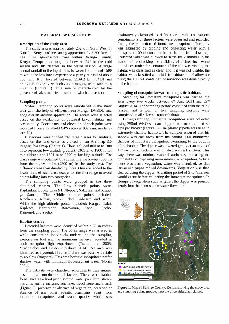
BONOROWO WETLANDS 8 (1): 25-32, June 2018
26
MATERIAL AND METHODS
Description of the study area
The study area is approximately 252 km, North West of
Nairobi, Kenya and measuring approximately 3,500 km2. It
lies in an agro-pastoral zone within Baringo County,
Kenya. Temperature range is between 24° in the cold
season and 30° degrees in the warm season. Average
annual rainfall in the highland is between 1000 m and 1500
m while the low lands experience a yearly rainfall of about
600 mm. It is located between 35.602 E, 0.541N and
36.277 E, 0.723 N with elevation ranging from 800 m to
2300 m (Figure 1). This area is characterized by the
presence of lakes and rivers, some of which are seasonal.
Sampling points
Sixteen sampling points were established in the study
area with the help of officers from Marigat DVBDU and
google earth android application. The scores were selected
based on the availability of potential larval habitats and
accessibility. Coordinates and elevation of each point were
recorded from a handheld GPS receiver (Garmin, model e-
trex 10).
Elevations were divided into three classes for analysis,
based on the land cover as viewed on an Arc map 3.0
imagery base map (Figure 1). They included 800 m to1300
m to represent low altitude gradient, 1301 m to 1800 m for
mid-altitude and 1801 m to 2300 m for high altitude. The
class range was obtained by subtracting the lowest (800 m)
from the highest point (2300 m) in the study area. The
difference was then divided by three. One was added to the
lower limit of each class except for the first range to avoid
points falling into two categories.
The sampling points were grouped in the three
altitudinal classes. The Low altitude points were,
Kapkuikui, Loboi, Lake 94, Nteppes, Salabani, and Kambi
ya Samaki. The Middle altitude points included:
Kipcherere, Kimau, Yomu, Sabor, Kabeswa, and Sabor.
While the high altitude points included: Kurget, Talai,
Kaplewa, Kaptimbor, Borowonin, Tandui, Sacho,
Kamonol, and Sacho.
Habitat census
Potential habitats were identified within a 50 m radius
from the sampling point. The 50 m range was arrived at
while considering individuals undertaking the sampling
exercise on foot and the minimum distance recorded in
adult mosquito flight experiments (Tsuda et al. 2008;
Verdonschot and Besse-Lototskaya 2014). An area was
identified as a potential habitat if there was water with little
to no flow (stagnant). This was because mosquitoes prefer
shallow water with minimum flow/stagnant water (Norris
2004).
The habitats were classified according to their nature,
based on a combination of factors. There were habitat
forms such as a hoof print, swamp, water pan, dam, stream
margins, spring margins, pit, lake, flood zone and marsh
(Figure 2), presence or absence of vegetation, presence or
absence of any other aquatic organisms apart from
immature mosquitoes and water quality which was
qualitatively classified as definite or turbid. The various
combinations of these factors were observed and recorded
during the collection of immature mosquitoes. Turbidity
was estimated by dipping and collecting water with a
transparent 100ml container in the habitat from down-up.
Collected water was allowed to settle for 2 minutes in the
bottle before checking the visibility of a three-inch white
tile placed under the container. If the tile was visible, the
habitat was classified as clear, and if it was not visible, the
habitat was classified as turbid. In habitats too shallow for
using the 100 mL container, observation was done directly
in the habitat.
Sampling of mosquito larvae from aquatic habitats
Sampling for immature mosquitoes was carried out
after every two weeks between 6th June 2014 and 28th
August 2014. The sampling period coincided with the rainy
season, and a total of five sampling sessions were
completed in all selected aquatic habitats.
During sampling, immature mosquitoes were collected
using 350ml WHO standard dippers at a maximum of 30
dips per habitat (Figure 3). The plastic pipette was used in
extremely shallow habitats. The sampler ensured that his
shadow was cast away from the habitat. This minimized
chances of immature mosquitoes swimming to the bottom
of the habitat. The dipper was lowered gently at an angle of
45⁰ so that collection was by displacement suction. This
way, there was minimal water disturbance, increasing the
probability of capturing more immature mosquitoes. Where
there was dense vegetation, water was disturbed, so that
larvae and pupae moved downwards. Vegetation was then
cleared using the dipper. A waiting period of 3 to 4minutes
would ensue before collecting the immature mosquitoes. In
clumps of vegetation such as grass, the dipper was pressed
gently into the plant so that water flowed in.
Figure 1. Map of Baringo County, Kenya, showing the study area
and sampling points grouped into the three altitudinal classes.

DANCAN – Vectors of malaria and rift valley fever along altitudinal gradient in Kenya
27
Figure 2. Images of different aquatic habitats: dam margin (A); animal hoof print (B); stream bank (C); Lake Flood zone (D); water pit
(E); mash (F); spring bank (G)
Figure 3. The researcher was inspecting the dipper for immature
mosquitoes
Figure 4. Collection cup was containing immature mosquitoes
(A), Algae in a habitat (B)
After collection, the immature mosquitoes were
transferred into a sealable collection cup using a plastic
pipette, or directly from the habitat onto a pipette and
finally into the sealable container. The collection cups were
filled with water sourced from respective sampled habitats
to avoid desiccation of the specimen. A pencil written
label, indicating the point and date of collection were
immersed into the cup before sealing and subsequent
transportation to the DVBDU laboratory in Marigat.
In the laboratory, third and fourth instar larvae were
identified (while still alive on a petri dish, using a
dissecting microscope), and separated from second and first
instar larvae. The third and fourth instar larvae were stored
in labeled, sealable cups containing 80% ethanol, waiting
A B C
D E F
G
A B

BONOROWO WETLANDS 8 (1): 25-32, June 2018
28
2
for identification to species level.
The first and second instar larvae were put in labeled
cups, three-quarter full of water from the source habitat
containing algae and loosely sealed to allow air in and out
(Figure 4). They were left at room temperature (an average
of 290C during the day) to allow development to the fourth
instar. Each cup contained not more than 12 larvae. An
experiment conducted a week before the first collection
showed that there is reduced development in instances
where there were more than 12 larvae in a cup. It was also
observed that development from second to fourth instar, at
room temperature, took a minimum of one and a maximum
of two days in a cup containing water and algae from the
source habitat compared to four days when tap water was
used.
Identification of larvae
Ethanol-preserved larvae were identified to species
level using third and fourth instar morphological keys
under guidance from experts in the Marigat DVBDU (Mark
Rotich and Richard Borr). This was by observing features
such as the color of the head, arrangement and shape of
abdominal setae, number and type of combs, distinct hairs
on the sandal, siphon index and other markings and
features on the body surface as guided by the identification
key (Gillies and de Meillon 1968). This was done under a
dissecting microscope.
Data analysis
Species diversity analysis was performed on PAST
version 2.17c. Other statistical studies were conducted on R
version 3.1.1. To standardize the abundance of a species
collected in each habitat, the total number of individuals
collected for that species in the habitat was divided by the
average number of dips in the habitat and the quotient
multiplied by 30. Thirty (30) was the maximum number of
dips for all habitats. Standardization ensured that figures
were comparable among all habitats. Comparison of
mosquitoes collected in different altitudinal classes was
made using the chi-square test. Generalized linear model
(GLM) was used to estimate the effect of various habitat
parameters on diversity and the abundance of species.
Linear correlation analysis was applied to evaluate the
association between altitude and the variety and
distribution of species in the study area.
RESULTS AND DISCUSSION
Diversity along the altitudinal gradient
A total of 1,536 immature mosquitoes were collected
from which 10 mosquito species were identified. With
respect to distribution along altitudinal gradients, 8 species
(Cx pipiens, Cx. quinquefaciatus, Cx. annulioris, Cx.
poicilipes, An. pharoensis, An. coustani. An. gambiae and
An. funestus) were found in altitudinal class range varying
between 800 m and 1300 m (Hˈ = 1.462), with 7 (Cx
pipiens, Cx. quinquefaciatus, Cx. annulioris, Cx. poicilipes,
An. pharoensis, An. coustani. and An. gambiae) found
between 1301 m and 1800 m (Hˈ = 1.686) and 9 species (Cx
pipiens, Cx. quinquefaciatus, Cx. annulioris, Cx. poicilipes,
An. pharoensis, Cx. tigripes, An. coustani, An. gambiae and
Ae. taylori) between 1801 m and 2300 m (Hˈ = 0.9836). Of
all the species identified, only seven species (Cx pipiens,
Cx. quinquefaciatus, Cx. annulioris, Cx. poicilipes, An.
pharoensis, An. coustani and An. gambiae) were common
in the three altitudinal zones, with An. funestus limited to
lower altitudinal zone while both Cx. tigripes and Ae.
taylori were found in higher altitudinal zones (1801m-2300
m) only. The Buza and Gibson evenness (e^Hˈ/S) showed
that the 1301 m to 1800 m altitudinal class had higher
regularity (0.77), followed by 800 m to 1300 m altitudinal
level (0.53), and 1801 m to 2300 m altitudinal class (0.3)
(Table 1).
Comparison of mosquitoes collected in different
altitudinal classes revealed variations in the respective
species counts (χ = 127.47; p-value < 0.001). There was,
however, no variation in the total number collected among
the different altitudinal classes (χ = 2.17; p-value = 0.34).
Of the 1,536 immature mosquitoes collected, Cx.
quinquefaciatus constituted 58.8%, dominating the species
community, while An. funestus made only 0.04% of the
total collection.
Distribution of mosquito species in the altitudinal ranges
The distribution of various species along the altitudinal
ranges was varied (Table 1). However, most of the species
showed no correlation with altitude. This is as described
below.
Culex species
Four Culex species were identified in both 800 m to
1300 m and 1301 m to 1800 m altitudinal ranges with five
Culex species identified in 1801 m to 2300 m altitudinal
range (Table 1). Culex species identified in 800 m to 1300
m included Cx. quinquefaciatus (886.6), Cx. pipiens
(206.3), Cx. annulioris (76.0) and Cx. poicilipes (18.8),
while Cx. quinquefaciatus (409.0), Cx. poicilipes (126.3),
Cx. pipiens (91.9) and Cx. annulioris (126.5) were
identified in 1301 m to 1800 m altitudinal range. The five
Culex species identified in 1801 m to 2300 m intervals
included Cx. quinquefaciatus (1684.2), Cx. pipiens (175.0),
Cx. annulioris (130.0), Cx. poicilipes (105.9) and Cx.
tigripes (24.9).
Cx. quinquefaciatus was the most abundant mosquito
species in the entire study area and the most abundant
Culex species in the three altitudinal class ranges. Culex
poicilipes was the least abundant in the class range between
800 m to 1300 m while Cx. annulioris and Cx. pipiens were
the least abundant in the altitudinal class range between
1301 m to 1800 m. Culex tigripes was only in the
altitudinal class range between 1801 m to 2300 m. It was
also the least abundant in this altitudinal class range (Table
1). Further analysis showed that none of the Culex species
had a significant correlation with altitude (p>0.05; Table 2).
Anopheles species
Distribution of Anopheles species in the altitudinal class
ranges was, An. pharoensis (385.2), An. coustani (108.7),
An. gambiae s.l (74.5) and An. funestus (18.0) between 800
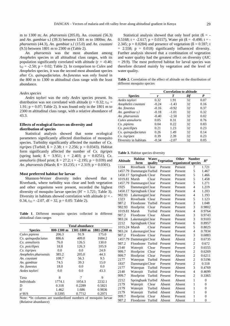
DANCAN – Vectors of malaria and rift valley fever along altitudinal gradient in Kenya
29
m to 1300 m; An. pharoensis (205.0), An. coustani (56.3)
and An. gambiae s.l (39.3) between 1301 m to 1800m; An.
pharoensis (44.3), An. gambiae s.l (15.0) and An. coustani
(9.5) between 1801 m to 2300 m (Table 2).
An. pharoensis was the most abundant among
Anopheles species in all altitudinal class ranges, with its
population significantly correlated with altitude (r = -0.40;
t32 = -2.50; p = 0.02; Table 2). In comparison to Culex and
Anopheles species, it was the second most abundant species
after Cx. quinquefaciatus. An.funestus was only found in
the 800 m to 1300 m altitudinal class range with the least
abundance.
Aedes species
Aedes taylori was the only Aedes species present. Its
distribution was not correlated with altitude (r = 0.32; t32 =
1.91; p = 0.07; Table 2). It was found only in the 1801 m to
2300 m altitudinal class range, with a relative abundance of
43.3.
Effects of ecological factors on diversity and
distribution of species
Statistical analysis showed that some ecological
parameters significantly affected distribution of mosquito
species. Turbidity significantly affected the number of Cx.
tigripes (Turbid; ß = 2.38; t = 2.256; p = 0.0343). Habitat
form significantly affected the number of Cx. tigripes
(spring bank; ß = 3.951; t = 2.403; p = 0.0251), Cx.
annulioris (Hoof print; ß = 27.2; t = -2.195; p = 0.039) and
An. pharoensis (Marsh; ß = 33.235; t = 2.319; p = 0.0301).
Most preferred habitat for larvae
Shannon-Weiner diversity index showed that a
Riverbank, where turbidity was clear and both vegetation
and other organisms were present, recorded the highest
diversity of mosquito larvae species (H' = 1.721; Table 3).
Diversity in habitats showed correlation with altitude (r = -
0.34, t32 = -2.07, df = 32, p = 0.05: Table 2).
Table 1. Different mosquito species collected in different
altitudinal class ranges
Total abundance
Species 800-1300 m 1301-1800 m 1801-2300 m
Culex pipiens 206.3 91.9 175.0
Cx. quinquefaciatus 886.6 409.0 1684.2
Cx. annulioris 76.0 126.5 130.0
Cx. poicilipes 18.8 126.3 105.9
Cx. tigripes 0.0 0.0 24.9
Anopheles pharoensis 385.2 205.0 44.3
An. coustani 108.7 56.3 9.5
An. gambiae 74.5 39.3 15.0
An. funestus 18.0 0.0 0.0
Aedes taylori 0.0 0.0 43.3
Taxa 8 7 9
Individuals 1774.1 1054.3 2232.1
D 0.318 0.2289 0.5821
Hˈ 1.462 1.686 0.9836
e^H/S 0.5395 0.7712 0.2971
Note: *In columns are standardized numbers of mosquito larvae
(Relative abundance)
Statistical analysis showed that only hoof print (ß = -
0.5168; t = -2.617; p = 0.0157), Water pit (ß = -0.498; t = -
2.345; p = 0.0284) and presence of vegetation (ß = 0.597; t
= 2.558; p = 0.018) significantly influenced diversity.
Further analysis showed that a combination of vegetation
and water quality had the greatest effect on diversity (AIC
= 29.9). The most preferred habitat for larval species was
therefore dictated mainly by vegetation and the level of
water quality.
Table 2. Correlation of the effect of altitude on the distribution of
different mosquito species
Correlation to altitude
Species r T Df P
Aedes taylori 0.32 1.91 32 0.07
Anopheles coustani -0.24 -1.43 32 0.16
An. fenestus -0.16 -0.92 32 0.37
An. gambiae s.l -0.18 -1.01 32 0.32
An. pharoensis -0.40 -2.50 32 0.02
Culex annulioris 0.05 0.31 32 0.76
Cx. pipiens 0.04 0.22 32 0.83
Cx. poicilipes 0.21 1.23 32 0.23
Cx. quinquefaciatus 0.26 1.49 32 0.14
Cx. tigripes 0.39 2.39 32 0.23
Diversity in habitats -0.34 -2.07 32 0.05
Table 3. Habitat species diversity
Altitude Habitat
form
Water
quality Vegetation
Other
organisms
Number
of species H1
1334 Riverbank Clear Present Present 7 1.721
1457.79 Dammargin Turbid Present Present 5 1.467
1450.17 Springbank Clear Present Present 5 1.466
1019.81 Marsh Clear Present Present 5 1.458
1457.79 Dammargin Clear Present Present 5 1.271
1925 Dammargin Clear Present Present 4 1.219
1450.17 Springbank Clear Present Present 4 1.203
982.93 Lakemargin Clear Present Present 4 1.193
1323 Riverbank Clear Present Present 5 1.123
987.2 Floodzone Turbid Present Present 3 1.048
982.93 Hoofprint Clear Present Present 3 0.9802
1019.81 Marsh Turbid Present Present 4 0.9764
987.2 Floodzone Clear Absent Absent 3 0.9743
983.24 Lakemargin Clear Present Present 3 0.9103
2212 Springbank Clear Present Present 6 0.8957
1015.24 Marsh Clear Present Present 5 0.8025
983.24 Lakemargin Clear Present Present 4 0.7834
987.2 Floodzone Clear Present Present 3 0.6883
1457.79 Dammargin Clear Absent Absent 2 0.6735
987.2 Floodzone Turbid Present Present 2 0.672
2140 Waterpit Clear Present Present 2 0.6555
999.7 Hoofprint Clear Present Present 2 0.6269
999.7 Hoofprint Clear Present Absent 2 0.6211
2177 Waterpan Turbid Present Absent 2 0.5196
1837 Dammargin Clear Present Present 2 0.518
2177 Waterpan Turbid Present Absent 3 0.4769
2140 Waterpit Turbid Present Present 4 0.4699
999.7 Hoofprint Turbid Present Present 2 0.3365
2212 Springbank Turbid Absent Absent 1 0
2179 Waterpit Clear Absent Absent 1 0
2179 Waterpit Turbid Absent Absent 1 0
2179 Waterpit Turbid Absent Absent 1 0
999.7 Hoofprint Clear Absent Present 1 0
987.2 Floodzone Turbid Absent Absent 1 0

BONOROWO WETLANDS 8 (1): 25-32, June 2018
30
Discussion
The only Aedes species identified was Ae. taylori in the
altitudinal range between 1801 m to 2300 m. This species
has been implicated as a vector of yellow fever in selvatic
transmission. Its ability to feed on monkeys and humans
enables it to spread the yellow fever virus from monkeys to
human beings (Digoutte 1999). Primary infections of RVF
are a result of floodwater Aedes species which are
considered as reservoir hosts of RVF virus due to trans-
ovarian transmission and ability of the eggs to diapause in
the soil for months or years until there is flooding (Sang et
al. 2010). Flood water Aedes species in Kenya include Ae.
mintoshi, Ae. ocharacieus, Ae. sudanensis, and Ae.
circumluteolus (Lutomiah et al. 2013).
None of these species were identified in the entire study
area within the study period. The results, therefore, indicate
that there was no risk of RVF first outbreak based on the
identified vectors in the study area during the study period.
This was consistent with Baringo county vector-borne
disease unit (VBDU) data and public health records. They
indicated no cases of RVF were reported between January
2013 and September 2014 within the study region.
The RVF virus has previously been isolated in all the
three genera identified in the study area (Sang et al. 2010).
Many species of mosquitoes and sandflies are susceptible
to RVF if they feed on an infected host and can cause
secondary transmission of the virus. The wide range of
such secondary vectors is what causes sudden epidemics of
the virus after primary infection by the flood water Aedes
species (Linthicum et al. 1985). This indicated that,
although there were no primary vector larvae species
identified in the study area, in case of entry of infected
individuals such as cattle into the region, there would be a
possible epidemic especially if this was in the rainy season
as mosquito species reach their peak abundances during
such seasons (Uyi 2013).
Among the identified 10 species, five were Culex
mosquito species; Cx quinquefaciatus, Cx. pipiens, Cx.
annulioris, Cx. poicilipes and Cx. tigripes. Apart from
being secondary vectors of RVF, anop species have been
implicated as vectors of various other arbovirus diseases.
An example of such a disease is the West Nile Virus. The
west Nile Virus is transmitted by Culex species, from birds
to humans and other mammals. This is a result of their
ability to feed on both mammals and birds (Molei et al.
2006). Evidence of the West Nile virus transmission in
Kenya was found in mosquitoes collected in various parts
including the former Rift valley province which Baringo,
currently Baringo County, was part of (LaBeaud et al.
2011). None of the Culex species showed a significant
correlation to altitude. This implied that in case of
emergence of RVF, West Nile Virus or any other disease
spread by the Culex species, whose distribution was not
limited by altitude, the disease might spread rapidly in the
entire county if rapid interventions are not initiated.
Culex quinquefaciatus was the most abundant species in
the study area, and Cx tigripes was the least abundant.
Culex quinquefaciatus, apart from being among secondary
vectors of RVF in epidemics in Kenya (Sang et al. 2010), it
is also the primary vector of urban lymphatic filariasis,
caused by the nematode Wuchereria bancrofti (Bockarie et
al. 2009). However, there are no cases of vector-
transmitted filariasis in Baringo County. Any examples that
come in are from the coastal regions of Kenya. Mosquito
species in the area are not able to transmit the disease
(unpublished data, Baringo County, VBDU). Culex tigripes
is a predator of other mosquito larvae and can be used as
larval biological control (Appawa et al. 2000). With the
increase in highland malaria all over Kenya and
considering it was in the high altitude regions, it can be
exploited as a measure of reducing highland malaria
transmission.
Like Cx. quinquefaciatus and Cx. tigripes, the other
three Culex species, Cx. pipiens, Cx. annulioris and Cx.
poicilipes did not show any significant correlation with
altitude. This is an indication that any diseases they
transmit can be spread both in the highlands and the
lowlands leading to infections in the entire region. Culex
pipiens was implicated as the primary vector maintaining
the RVF epidemic in Egypt from 1971 to 1978 (Hoogstraal
et al. 1979). The laboratory test of Cx. pipiens strains have
also shown that apart from being susceptible to RVF virus,
they are also vulnerable to West Nile Virus (Amraoui et al.
2012). It is also a primary vector of the Ndumu Virus
(NDUV) as reported in a study done in Garissa, Kenya,
where evidence of trans-ovarian transmission of the virus
was recorded (Lutomiah et al. 2014). Studies in Senegal
indicated that Cx. poicilipes was the main RVF virus vector
after the 1998 outbreak in Mauritania (Diallo et al. 2000).
RVF viruses were isolated from Cx. annulioris species in
the 2007/2008 epidemic in Kenya (Sang et al. 2010). These
are further indications that all the Culex species identified
in the study area are secondary vectors of RVF and
therefore the fact that elevation does not limit them
indicates that all regions of Baringo County have a
potential risk of RVF secondary outbreaks.
Among the four Anopheles species identified in the
study area, only An. pharoensis showed a significant
correlation with altitude. However, between the altitudinal
classes, the least abundances of Anopheles species were in
the high altitude class (1801-2300 m). Anopheles
pharoensis was the most abundant Anopheles species and
second most abundant after Cx. quinquefaciatus amongst
all species identified in the study area. This is contrary to
what a study in 2011 established, where a sibling species of
An. gambiae s.l, and An. arabiensis was the most abundant
(Mala et al. 2011). Anopheles pharoensis has been
documented as an efficient malaria vector in Senegal
(Carrara et al. 1990). It might also be an efficient vector in
Baringo County considering the many cases of malaria,
which were higher during the study period (Unpublished
data, Baringo county public health records). Studies on its
biting habits in Kapkuikui village, Baringo County
indicated that it bites more often outdoor than indoor and is
exophilic (Aniedu 1993). This might be the reason for its
success since interventions in Baringo County mostly
involve the use of insecticide-treated bed nets and
pyrethrum spraying inside houses. These affect indoor
bitters. Anopheles funestus and An. gambiae s.l are
documented as endophilic and prefer biting indoors than
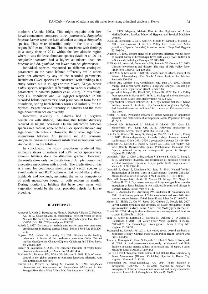
DANCAN – Vectors of malaria and rift valley fever along altitudinal gradient in Kenya
31
outdoors (Aniedu 1993). This might explain their low
larval abundances compared to An. pharoensis. Anopheles
funestus larvae were the least abundant amongst Anopheles
species. They were identified only in the low altitude
region (800 m to 1300 m). This is consistent with findings
in a study done in 2011 within the low altitude region
where it was the least abundant species (Mala et al. 2011).
Anopheles coustani had a higher abundance than An.
funestus and An. gambiae, but lower than An. pharoensis.
Individual species responded to different ecological
parameters in the same habitat differently while others
were not affected by any of the recorded parameters.
Results on Culex species are consistent with findings in a
study carried out in villages within Mwea, Kenya, where
Culex species responded differently to various ecological
parameters in habitats (Muturi et al. 2007). In this study,
only Cx. annulioris and Cx. tigripes responded to the
recorded habitat parameters; hoof print habitat form for Cx.
annulioris, spring bank habitats form and turbidity for Cx.
tigripes. Vegetation and turbidity in habitats had the most
significant influence on diversity.
However, diversity in habitats had a negative
correlation with altitude, indicating that habitat diversity
reduced as height increased. On the interaction between
species in a habitat, none of the Culex species showed any
significant interactions. However, there were significant
interactions between An. funestus and An. coustani.
Anopheles pharoensis showed substantial interactions with
An. coustani in the habitats.
In conclusion, the study hypothesis predicted that
immature stages of malaria and RVF vector species vary
amongst habitats along the altitudinal gradient. However,
the results show only the distribution of An. pharoensis had
a negative association with altitude. The implication of this
is a need for continuous monitoring of vector species to
avoid malaria and RVF outbreaks that would likely affect
highlands and lowlands, assuming the vector competence
of adult mosquitoes found in both regions is similar.
During monitoring, habitats that have clear water with
vegetation would be the most probable culprit for larvae
breeding.
REFFERENCE
Amraoui F, Krida G, Bouattour A, Rhim A, Daaboub J, Harrat Z, Failloux
AB. 2012. Culex pipiens, an experimental efficient vector of West Nile and Rift Valley fever viruses in the Maghreb region. PloS One 7:
e36757. DOI: 10.1371/journal.pone.0036757
Aniedu I. 1997. Dynamics of malaria transmission near two permanent breeding sites in Baringo district, Kenya. Indian J Med Res 105: 206-
211.
Appawu MA, Dadzie SK, Quartey SQ. 2000. Studies on the feeding behaviour of larvae of the predaceous mosquito Culex (Lutzia)
tigripes Grandpre and Chamoy (Diptera: Culicidae). Intl J Trop Insect
Sci 20: 245-250. Bacaer N, Guernaoui S. 2006. The epidemic threshold of vector-borne
diseases with seasonality. J Math Biol 53: 421-436
Bockarie MJ, Pedersen EM, White GB, Michael E. 2009. Role of vector control in the global program to eliminate lymphatic filariasis. Ann
Rev Entomol 54: 469-487.
Carrara GC, Petrarca V, Niang M, Coluzzi M. 1990. Anopheles pharoensis and transmission of Plasmodium falciparum in the
Senegal River delta, West Africa. Med Vet Entomol 4: 421-424.
Cox J. 1999. Mapping Malaria Risk in the Highlands of Africa.
MARA/Durban. London School of Hygiene and Tropical Medicine,
London. Diallo M, Lochouarn L, Ba K, Sall AA, Mondo M, Girault L, Mathiot C.
2000. First isolation of the Rift Valley fever virus from Culex
poicilipes (Diptera: Culicidae) in nature. Amer J Trop Med Hygiene 62: 702-704.
Digoutte JP. 1999. Present status of an arbovirus infection: yellow fever,
its natural history of hemorrhagic fever, Rift Valley fever. Bulletin de la Societe de Pathologie Exotique 92: 343-348.
El Vilaly AE, Arora M, Butterworth MK, Jarnagin W, Comrie AC. 2013.
Climate, environment and disease: The case of Rift Valley fever. Progr Phys Geogr 37 (2): 259-269.
Gillies MT, de Meillon B. 1968). The anophelinae of Africa, south of the
Sahara. Johannesburg: The South African Institute for Medical Research 220-330
Githeko AK, Lindsay SW, Confalonieri UE, Patz JA. 2000. Climate
change and vector-borne diseases: a regional analysis. Bulleting of World Health Organization 78 n.9 Genebra Jan.
Hoogstraal H, Meegan JM, Khalil GM, Adham FK. 1979. The Rift Valley
fever epizootic in Egypt 1977–1978: 2. Ecological and entomological studies. Trans R Soc Trop Med Hygiene 73: 624-629.
Kenya Medical Research Institute. 2014. Kenya malaria fact sheet. Kenya
medical research institute, http://www.kemri.org/index.php/help-desk/search/diseases-a-conditions/29- malaria/113-kenya-malaria-
fact-sheet.
Kiritani K. 2006. Predicting impacts of global warming on population dynamics and distribution of arthropods in Japan. Population Ecology
48: 5-12.
LaBeaud AD, Sutherland LJ, Muiruri S, Muchiri EM, Gray LR, Zimmerman PA, King CH. 2011. Arbovirus prevalence in
mosquitoes, Kenya. Emerg Infect Dis 17: 233-241.
Li Z, He Y, Winfred H, Wang X, Zhang W, Cao W, Du J, Xin H, Chang L. 2012. Altitude dependency of trends of daily climate extremes in
southwestern China, 1961–2008. J geographical science 22: 416-430.
Linthicum KJ, Davies FG, Kairo A, Bailey CL. 1985. Rift Valley fever
virus (family Bunyaviridae, genus Phlebovirus). Isolations from
Diptera collected during an inter-epizootic period in Kenya. J Hygiene 95: 197-209.
Lutomiah J, Bast J, Clark J, Richardson J, Yalwala S, Oullo D, Sang R.
2013. Abundance, diversity, and distribution of mosquito vectors in selected ecological regions of Kenya: public health implications. J
Vector Ecol 38: 134-142.
Lutomiah J, Ongus J, Linthicum KJ, Sang R. 2014. Natural Vertical Transmission of Ndumu Virus in Culex pipiens (Diptera: Culicidae)
Mosquitoes Collected as Larvae. J Med Entomol 51: 1091-1095.
Mala AO, Irungu LW, Shililu JI, Muturi EJ, Mbogo CC, Njagi JK, Githure JI. 2011. Dry season ecology of Anopheles gambiae complex
mosquitoes at larval habitats in two traditionally semi-arid villages in
Baringo, Kenya. Parasit Vect 4: 1-11. Molaei G, Andreadis TG, Armstrong PM, Anderson JF, Vossbrinck CR.
2006. Host feeding patterns of Culex mosquitoes and West Nile virus
transmission, northeastern United States. Emerg Infect Dis 12: 468-474. Muturi EJ, Shililu JI, Gu W, Jacob BG, Githure JI, Novak RJ. 2007.
Larval habitat dynamics and diversity of Culex mosquitoes in rice
agro-ecosystem in Mwea, Kenya. Amer J Trop Med Hygiene 76: 95-102. Norris DE. 2004. Mosquito-borne diseases as a consequence of land use
change. EcoHealth 1: 19-24.
Sang R, Kioko E, Lutomiah J, Warigia M, Ochieng C, O’Guinn M, Richardson J. 2010. Rift Valley Fever Virus Epidemic in Kenya,
2006/2007: The Entomologic Investigations. Amer J Trop Med
Hygiene 83: 28–37. Swanepoel R, Paweska JT. 2011. Rift valley fever. Oxford textbook of
Zoonoses: Biology, Clinical Practice, and Public Health. Oxford Univ
Press, London. Tsuda Y, Komagata O, Kasai S, Hayashi T, Nihei N, Saito K, Kobayashi
M. 2008. A mark-release-recapture study on dispersal and flight
distance of Culex pipiens pallens in an urban area of Japan. J Amer Mosquito Control Assoc 24:339-343.
Uyi COO. 2013. Temporal Distribution of and Habitat Diversification by
Some Mosquitoes (Diptera: Culiciclae) Species in Benin City, Nigeria. J Entomol 10: 13-23.
Verdonschot PF, Besse-Lototskaya AA. 2014. Flight distance of
mosquitoes (Culicidae): A metadata analysis to support the management of barrier zones around rewetted and newly constructed
wetlands. Limnol Ecol Manag Inland Waters 45: 69-79.

BONOROWO WETLANDS 8 (1): 25-32, June 2018
32
Wettstein W, Schmid B. 1999. Conservation of arthropod diversity in
montane wetland; effects of altitude, habitat quality and habitat
fragmentation on butterflies and grasshoppers. J Appl Ecol 36: 363-373.
Woods CW, Karpati AM, Grein T, McCarthy N, Gaturuku P, Muchiri E,
World Health Organization Hemorrhagic Fever Task Force. 2002. An outbreak of Rift Valley fever in northeastern Kenya. 1997-98. Emerg
Infect Dis 8: 138-144.
World Health Organization. 1975. Manual on practical entomology in
malaria. WHO, Geneva.
World Health Organization. 2007. Rift Valley Fever in Kenya, Somalia and the United Republic of Tanzania. World Health Organization
Global alert and response. WHO, Geneva
World Health Organization. 2013a. Malaria entomology and vector control. World Health Organization, Geneva.
World Health Organization. 2013b. Malaria report. World Health
Organization, Geneva.
BONOROWO WETLANDS P-ISSN: 2088-110X Volume 8, Number 1, June 2018 E-ISSN: 2088-2475
Pages: 33-41 DOI: 10.13057/bonorowo/w080104
Influence of human activity on diversity and abundance of insects in
three wetland environments in Ghana
BEATRICE AYORKOR MENSAH1, ROSINA KYEREMATEN2,, TED ANNANG1,
SAMUEL ADU-ACHEAMPONG3 1Institute of Environment and Sanitation Studies (IESS), University of Ghana, Legon, Ghana
2Department of Animal Biology and Conservation Science, University of Ghana, Legon, Ghana. ♥email: [email protected] 3Department of Agronomy, University for Development Studies, P.O. TL Box 1982 Nyankpala-Tamale, Ghana
Manuscript received: 2 April 2018. Revision accepted: 22 June 2018.
Abstract. Mensah BA, Kyerematen R, Annang T, Adu-Acheampong S. 2018. Influence of human activity on diversity and abundance of
insects in three wetland environments in Ghana. Bonorowo Wetlands 2: 33-41. The Wetland environment is unique with unique biota
that includes insects. Insects serve as indicators of environmental health, nevertheless, the recent spate of human encroachment on
wetlands is likely to affect its unique biotic composition, and this phenomenon poses a threat to the wetland environment. The physical
and chemical quality of studied habitats in this research provided background information for comparison against the established quality
standard of the wetland environment. The study involved reconnaissance surveys, insect trapping and social surveys on the impact of
anthropogenic activities on insect diversity and abundance in and around the wetland environment. Twenty-two insect orders belonging
to 112 families were sampled from different sites along the Sakumono, Kpeshie, and Muni-Pomadze wetlands. Species diversity and
abundance were significantly different among the various locations with the most diverse being Kpeshie. Water within wetlands in
Kpeshie was the most polluted although it had a positive correlation with insect diversity and abundance. Results of a survey of selected
communities showed that majority of the residents had a low level of education with less appreciation of issues involving the
environment including pollution. Majority of people within the surveyed communities were unable to access decent toilet facilities and
publicly demarcated waste disposal sites. There was no coordinated and concerted effort to manage these three wetlands two of which
are designated Ramsar sites. Activities such as farming, discharge of domestic garbage, improper fishing practices, improper disposal of
industrial and human waste are increasing the pollution risk of these wetland environments.
Keywords: Abundance, diversity, insect, lagoon, wetland
INTRODUCTION
Wetlands are highly diverse habitats and are known to
be among the earth’s most productive ecosystems (Barbier
et al. 1997). Wetlands can be classified based on their (i)
components (biotic and abiotic features), (ii) functions (the
interactions between the components such as nutrient
cycling), and (iii) attributes such as species diversities.
These characteristics of wetlands support human existence
and their related economic activities. “Wetlands” is an
elastic term which includes large variety of landforms.
Some cold climate wetlands are unique and thus have no
tropical equivalence, and vice versa. Tundras and
mangroves, for instance, are unique to the temperate and
tropics respectively.
Wetland resources comprise of the water, land, soils,
plants, and animals, which may be exploited for
subsistence, income, and employment. While wetland
services such as maintenance of hydrological and
biogeochemical cycles, act as management schemes for silt
and other materials, erosion control plays a dominant role
in maintaining the general ecological balance. For instance,
it has been reported that rivers and wetlands around Lake
Victoria act as natural purifiers (Scheren et al. 2000).
Besides supplying local communities with resources for
subsistence, wetlands support distant communities with
ecological services such as flood and water flow regulation
and drought alleviation, ground-water recharge, water
quality protection and purification, drinking water supply
and storage, erosion and sediment control, wastewater
treatment, carbon retention and climate modification
(Seyam et al. 2001). The New Partnership for Africa’s
Development (NEPAD) has identified six sectoral priorities
that include the Environment Initiative in Africa which
included wetland conservation which is recognized as one
of the eight sub-themes for priority intervention (Anon
2001).
Insects are vital for ecosystems functioning (Samways
et al. 2010). They can inhabit all conceivable habitats from
the pole to the equator and occupy all trophic niches more
than the level of primary producers (Resh and Carde 2003).
Insects are known to be the most abundant and diverse
organisms present in most environments. Insects may be
used as indicators of environmental quality (Kyerematen et
al. 2014 a, b; 2018 a, b; Acquah Lamptey et al. 2013 a, b,
Adu-Acheampong et al. 2016) due to their short life cycles
and sensitivity to perturbations. In most terrestrial
ecosystems, insects are the dominant herbivores. They may
significantly influence the plant community as well as
reflect the variety of plant resources available to them
(Barbour et al. 1998; Groves 2002). Insects in wetlands are
abundant and diverse because wetlands have too shallow
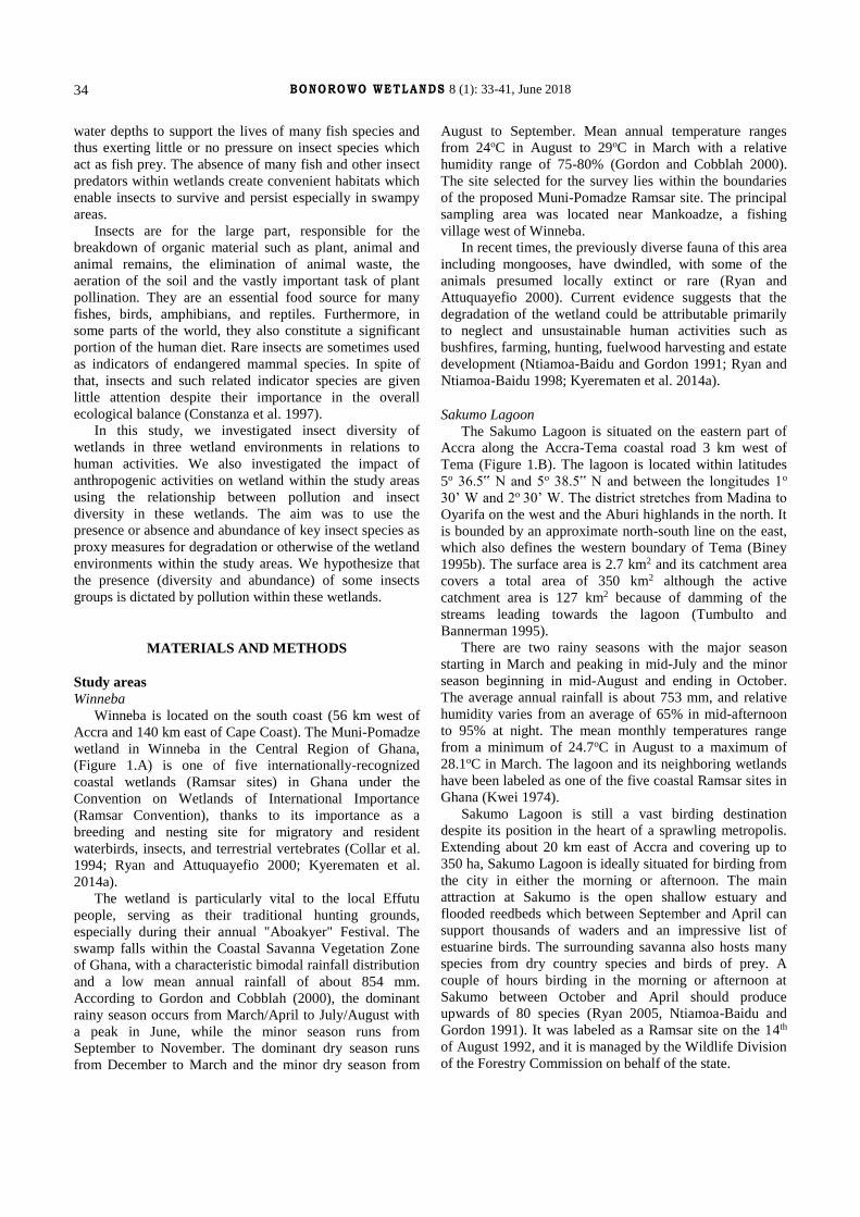
BONOROWO WETLANDS 8 (1): 33-41, June 2018
34
water depths to support the lives of many fish species and
thus exerting little or no pressure on insect species which
act as fish prey. The absence of many fish and other insect
predators within wetlands create convenient habitats which
enable insects to survive and persist especially in swampy
areas.
Insects are for the large part, responsible for the
breakdown of organic material such as plant, animal and
animal remains, the elimination of animal waste, the
aeration of the soil and the vastly important task of plant
pollination. They are an essential food source for many
fishes, birds, amphibians, and reptiles. Furthermore, in
some parts of the world, they also constitute a significant
portion of the human diet. Rare insects are sometimes used
as indicators of endangered mammal species. In spite of
that, insects and such related indicator species are given
little attention despite their importance in the overall
ecological balance (Constanza et al. 1997).
In this study, we investigated insect diversity of
wetlands in three wetland environments in relations to
human activities. We also investigated the impact of
anthropogenic activities on wetland within the study areas
using the relationship between pollution and insect
diversity in these wetlands. The aim was to use the
presence or absence and abundance of key insect species as
proxy measures for degradation or otherwise of the wetland
environments within the study areas. We hypothesize that
the presence (diversity and abundance) of some insects
groups is dictated by pollution within these wetlands.
MATERIALS AND METHODS
Study areas
Winneba
Winneba is located on the south coast (56 km west of
Accra and 140 km east of Cape Coast). The Muni-Pomadze
wetland in Winneba in the Central Region of Ghana,
(Figure 1.A) is one of five internationally-recognized
coastal wetlands (Ramsar sites) in Ghana under the
Convention on Wetlands of International Importance
(Ramsar Convention), thanks to its importance as a
breeding and nesting site for migratory and resident
waterbirds, insects, and terrestrial vertebrates (Collar et al.
1994; Ryan and Attuquayefio 2000; Kyerematen et al.
2014a).
The wetland is particularly vital to the local Effutu
people, serving as their traditional hunting grounds,
especially during their annual "Aboakyer" Festival. The
swamp falls within the Coastal Savanna Vegetation Zone
of Ghana, with a characteristic bimodal rainfall distribution
and a low mean annual rainfall of about 854 mm.
According to Gordon and Cobblah (2000), the dominant
rainy season occurs from March/April to July/August with
a peak in June, while the minor season runs from
September to November. The dominant dry season runs
from December to March and the minor dry season from
August to September. Mean annual temperature ranges
from 24oC in August to 29oC in March with a relative
humidity range of 75-80% (Gordon and Cobblah 2000).
The site selected for the survey lies within the boundaries
of the proposed Muni-Pomadze Ramsar site. The principal
sampling area was located near Mankoadze, a fishing
village west of Winneba.
In recent times, the previously diverse fauna of this area
including mongooses, have dwindled, with some of the
animals presumed locally extinct or rare (Ryan and
Attuquayefio 2000). Current evidence suggests that the
degradation of the wetland could be attributable primarily
to neglect and unsustainable human activities such as
bushfires, farming, hunting, fuelwood harvesting and estate
development (Ntiamoa-Baidu and Gordon 1991; Ryan and
Ntiamoa-Baidu 1998; Kyerematen et al. 2014a).
Sakumo Lagoon
The Sakumo Lagoon is situated on the eastern part of
Accra along the Accra-Tema coastal road 3 km west of
Tema (Figure 1.B). The lagoon is located within latitudes
5o 36.5‟ N and 5o 38.5‟ N and between the longitudes 1o
30’ W and 2o 30’ W. The district stretches from Madina to
Oyarifa on the west and the Aburi highlands in the north. It
is bounded by an approximate north-south line on the east,
which also defines the western boundary of Tema (Biney
1995b). The surface area is 2.7 km2 and its catchment area
covers a total area of 350 km2 although the active
catchment area is 127 km2 because of damming of the
streams leading towards the lagoon (Tumbulto and
Bannerman 1995).
There are two rainy seasons with the major season
starting in March and peaking in mid-July and the minor
season beginning in mid-August and ending in October.
The average annual rainfall is about 753 mm, and relative
humidity varies from an average of 65% in mid-afternoon
to 95% at night. The mean monthly temperatures range
from a minimum of 24.7oC in August to a maximum of
28.1oC in March. The lagoon and its neighboring wetlands
have been labeled as one of the five coastal Ramsar sites in
Ghana (Kwei 1974).
Sakumo Lagoon is still a vast birding destination
despite its position in the heart of a sprawling metropolis.
Extending about 20 km east of Accra and covering up to
350 ha, Sakumo Lagoon is ideally situated for birding from
the city in either the morning or afternoon. The main
attraction at Sakumo is the open shallow estuary and
flooded reedbeds which between September and April can
support thousands of waders and an impressive list of
estuarine birds. The surrounding savanna also hosts many
species from dry country species and birds of prey. A
couple of hours birding in the morning or afternoon at
Sakumo between October and April should produce
upwards of 80 species (Ryan 2005, Ntiamoa-Baidu and
Gordon 1991). It was labeled as a Ramsar site on the 14th
of August 1992, and it is managed by the Wildlife Division
of the Forestry Commission on behalf of the state.

MENSAH et al.-Influence of human activities on wetlands diversity
35
Figure 1. Map of the study area in Muni-Pomadze Lagoon (Winneba) (A), Kpeshie Lagoon (B), Sakumono Lagoon (C) and Ghana
A
B
C
C
A
B

BONOROWO WETLANDS 8 (1): 33-41, June 2018
36
Kpeshie Lagoon
The Kpeshie lagoon catchment area lies between
latitude 5º 33ʹ0 N and 5º 36ʹ20 N and stretches between
longitude 0º 9‟30‟ Wʹand 0º 7ʹ10‟ W (Figure 1.C). The
catchment area occupies almost 47.391551 ha. The
Kpeshie lagoon is less than 1km2 in surface area, and it is
situated along the outskirts of La, a peri-urban township.
The Municipal Assembly share boundaries with the
following Sub Metros: Osu Clottey towards the east,
Ayawaso towards the north, and Teshie to the west (Kpanja
2006).
Methods
Sampling points
Sampling points capture the main activities carried out
along the stretch of the lagoons which would affect the
water quality and insect diversity.
Sampling design and technique
The following trapping techniques were used to capture
insects: malaise traps, yellow pan traps, light traps, fruit-
baited charaxes traps, pitfall traps, flight interception traps,
sweep nets and aerial nets. A regular, perpendicular walk
was undertaken from predetermined sites to all the selected
locations along the lagoons. To ensure that the traps were
proportionally spaced, a meter tape was used to measure
the distance between them. The smallest intersite distance
was 50m with the largest being 250m. Where necessary a
hoe and machete were utilized to cut through grass or
mangrove to gain access. Sampling was done monthly
during the rainy season (April to June) and the dry season
(December to February) and the temperature was recorded
during these seasons.
Malaise trap
This trap has been designed to collect flying insects.
This rectangular tent-like trap made of black nylon netting
directs the flying insects into a collecting bottle containing
70% alcohol at the top end of one side. Insects were
collected after 3-5 days for subsequent identification.
Pitfall trap
This is used for trapping ground inhabiting insects and
is a straight-sided container that is sunk level with the
surface of the neighboring substratum. Ten traps were set at
20m intervals along the 200m transect in each area. Each
trap contained a soapy solution to break the surface tension
so that trapped insects would not be able to fly or crawl
out. Trapped insects were collected after 3-5 days and
emptied into a container containing 70% alcohol for
subsequent identification.
Yellow pan trap
Yellow pan traps collect insects that are attracted to the
yellow color filled with soapy water. Ten traps were set at
20m intervals along the 200m transect in each area.
Trapped insects were collected after 3-5 days and emptied
into plastic bottles containing 70% alcohol for subsequent
identification.
Flight interception trap
This trap is commonly used to intercept flying insects
which are not likely to be drawn to baits or light and is
assembled of brightly colored netting. Intercepted insects
fall into the trays at the bottom that contain a killing agent.
One trap was set in each area. Trapped insects were
collected after 3-5 days and emptied into bags containing
70% alcohol for subsequent identification.
Charaxes trap
This trap is made up of a net with a rectangular cross-
section with a string attached to the four corners at the
closed top and a flat wooden board connected at the open
end. Bait made up of mashed rotten banana mixed with
palm wine was placed on the board. Alcohol-loving insects
are mostly trapped by this method. Individual traps within
areas were separated from each other by at least 50m and
by no more than 250m (Oduro and Aduse-Poku 2005).
Standard field handling of specimens captured from
charaxes traps consisted of firmly squeezing the thorax to
disable the sample (Oduro and Aduse-Poku 2005).
Sweep net
The sweep net consists of a circular metallic rim with a
cloth attached to form a sac with the rim as the opening
with a wooden handle attached to the rim. It was swung
through the vegetation with the alternating forehand and
backhand strokes about 10 times and the content carefully
emptied into a killing jar. The catches were later transferred
into a bag containing 70% alcohol for subsequent
identification.
Aerial net
The aerial net consisted of a metallic rim with a wooden
handle and a fine mesh forming a sack. Swarming
butterflies, dragonflies and moths were spotted and
collected. The butterflies caught were placed in glassine
envelopes with wings folded together. This technique
prevented the insects from losing their scales, a feature
very vital for identification. The other insects were
transferred into killing jars containing ethyl acetate and
kept in glassine envelopes for later identification.
Visual observation and direct counts
Visual counts were done whenever an insect was
spotted that was out of reach to be collected or trapped. At
each site, random walk sampling was used for a minimum
of two hours to sample each site twice daily. This was done
under sunny conditions mostly between the hours of 8:00
hours GMT and 16:00 hours GMT. The butterflies were
identified by their wing patterns and colors as well as flight
patterns.
Social survey
Sampling technique
This study employed a purposive sampling technique,
the non-probability sampling technique.

MENSAH et al.-Influence of human activities on wetlands diversity
37
Questionnaire administration
Questionnaires were administered in the major
towns/settlements where water samples were collected in a
purposive sampling and non-probability technique. A total
of 280 questionnaires were administered in Winneba,
Sakumono, and Kpeshie. An effort was made to interview
women and men equally in each locality.
Interview
Interviews were conducted by interacting with some of
the locals in sensitive areas such as the small-scale
industries and the lagoon sites.
Non-participatory observations
Non-participatory observations were also undertaken to
enable the interviewer to generate initial information to
complement the data obtained from respondents.
Sorting and species identification
All insects sampled were either placed in containers
containing 70% alcohol or envelops and labeled for further
identification. All insects were identified to specific level
with reference to Museum collections in the Biodiversity
Museum of the Department of Animal Biology and
Conservation Science, University of Ghana, Legon, Scholtz
and Holm (2005), Carter et al. (1992), Gullan and Craston
(2005), and Boorman (1981).
Statistical analyses
Several statistical analyses were performed using SPSS
(Vol.16.0) to determine if some of these environmental
factors affected insect diversity within the wetlands. Data
obtained from the traps at a given sampling point on a
specific date were pooled to generate a single sample for
each site-data combination. Data from all the traps were
combined to get total insect diversity per study site and
sampling period. Simpson's Index (D) Shannon-Weiner
Index (H), Margalef index and the Pielou‟s Evenness index
(“J‟) were computed for measuring insect diversity.
A one-way ANOVA of insect diversity between groups
of wetlands was performed to test whether there was a
difference in insect diversity among the three sites (Muni-
Pomadze, Sakomo lagoon, and Kpeshie lagoon).
Simpson/Shannon diversity indices and Margalef richness
index were calculated. Nonparametric richness estimators
were applied to estimate total species richness at a site:
ACE (Abundance-based coverage estimator), ICE
(Incidence-based coverage estimator), Chao1 (Abundance-
based coverage estimator), Chao2 (Incidence-based
coverage estimator), Jack1 (First-order jackknife estimator)
and jack2 (Second-order jackknife estimator).
RESULTS AND DISCUSSION
Relative abundance of insects
As many as 5,541 individual insects were recorded
from all the three sites combined. Muni-Pomadze recorded
1,883, Sakumo wetlands recorded 1,530 and Kpeshie
recorded 2,128. Four hundred and twenty-nine species of
insects, belonging to 22 orders and 112 families were
collected from all three sites. Insects belonging to the
orders Hymenoptera, Diptera, Hemiptera, and Coleoptera
were the most abundant and diverse in all three areas
(Table 1). Hymenoptera and Diptera had the highest
relative abundances of 34% and 30% respectively during
the dry season. Meanwhile, Hymenoptera and Hemiptera
were dominant with relative abundances of 25% and 19%
respectively for the wet season.
There was no significant difference between Sakumo
and Kpeshie sites, but Muni-Pomadze was significantly
different from the two. The average of at least two groups
of the analysis differed significantly (p>0.05). The
abundance of insects did not vary much between Kpeshie
and Sakumo, but that of Muni-Pomadze was relatively less
than both Kpeshie and Sakumo, however, there was a
significant difference in the relative abundance of insects
sampled during the dry and the wet season. At all sampling
sites, the number of individual insects collected in the wet
season was higher than the dry season (Table 1).
Hymenoptera was the richest order in both seasons at
Sakumono with a relative abundance of 29.9% for the wet
season and 9.0% for the dry season. Kpeshie recorded an
overall relative abundance of 88% in the wet season and
12% in the dry season with Muni-Pomadze recording a
total relative abundance of 84% in the wet season and
15.6% in the dry season.
Species richness and diversity indices
Species richness in terms of Margalef and Pielou
indices were higher in the wet seasons at all three sites than
the dry seasons, but the Shannon Weiner and Simpsons
diversity indices were somewhat higher in the dry season
than that of the wet season (Table 2).
Observed species richness
Table 3 shows that the observed species richness (Sobs)
was higher at Kpeshie than the rest of the sites. The species
accumulation curves were approaching an asymptote, an
indication that species saturation had been reached and
sampling efforts were adequate.
Social survey: Respondent information
Sex
The questionnaires were administered in Sakumono, La
Trade Fair Area (Kpeshie) and Mankoadze (Muni-
Pomadze) in Winneba. The distribution of the polls was
done to ensure that there were an almost equal number of
men (137) and women (143). The population tested in each
of these locations was categorized according to the level of
activities carried out by residents in these catchment areas.
There were 100 respondents each from Sakumono and
Mankoadze constituting 71.4% of the total respondents for
each of the two sites. The rest of the respondents were from
the Trade Fair Area (Kpeshie), representing 28.6% of the
280 people sampled for the study. Forty-six percent and
42% of respondents from Trade Fair and Mankoadze
respectively disposed of their refuse indiscriminately
(Figure 2).

BONOROWO WETLANDS 8 (1): 33-41, June 2018
38
Table 1. Relative abundance of individual insects captured by order from the three wetlands
Order Sakumono Kpeshie Muni-Pomadze Relative abundance %
Coleoptera 93 218 372 12
Diptera 256 524 299 20
Hymenoptera 595 518 400 27
Hemiptera 188 415 214 15
Lepidoptera 105 112 145 7
Orthoptera 89 69 96 4.6
Dictyoptera 33 36 36 2
Collembola 51 54 79 3
Dermaptera 3 3 14 0.4
Odonata 15 14 33 1
Ephemeroptera 6 6 17 0.5
Mallophaga 0 0 9 0.1
Embioptera 3 0 14 0.3
Psocoptera 26 17 43 1.5
Neuroptera 18 18 16 0.9
Trichoptera 6 23 26 0.9
Thysanopter 18 58 43 2.2
Mecoptera 0 4 5 0.1
Isoptera 10 21 5 0.7
Anoplura 0 4 0 0.07
Homoptera 14 4 14 0.6
Plecoptera 1 0 3 0.07
Total individual number (N) 1530 2118 1883 100
Table 2. Diversity and richness indices for each season in and around each lagoon
Sites Simpson (I/D) Shannon-Weiner (H) Margalef (D) Pielou (J)
Wet Dry Wet Dry Wet Dry Wet Dry
Sakumono 10.8 13.10 4.15 3.57 131.9 58.8 0.8 0.87
Kpeshie 21.32 51.19 4.87 4.33 152.9 60.8 0.97 1.05
Muni-Pomadze 4.84 14.94 2.55 3.65 139.9 55.8 0.52 0.9
Table 3. Species richness estimates at all three sites
Sites Total Species Trapped
(Sobs)
Singleton/
doubleton Unique/duplicates ACE/ ICE Chao 1/ Chao 2 Jack 1/ Jack 2
Sakumono 199 79/48 19/35 246/785 264/204 218/202
Keshie 214 94/51 25/56 268/814 231/219 239/212
Muni-Pomadze 196 81/67 19/51 192/598 244/199 215/183
Table 4. Educational level breakdown
Educational Level Sakumono La Trade Fair Mankoadze Percentage (%) Total
Primary 15 8 23 16.4 46
Middle/JHS 24 18 25 23.9 67
Secondary/SSS 22 20 20 22.14 62
Voc/Com/Tech 16 15 14 16.1 45
Tertiary 14 17 9 14.3 40
No formal education 9 2 9 7.14 20
Total 100 80 100 100 280
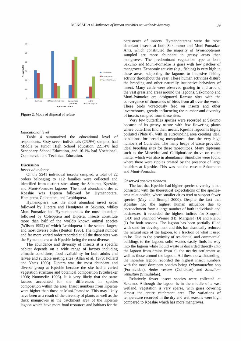
MENSAH et al.-Influence of human activities on wetlands diversity
39
Figure 2. Mode of disposal of refuse
Educational level
Table 4 summarized the educational level of
respondents. Sixty-seven individuals (23.9%) sampled had
Middle or Junior High School education, 22.14% had
Secondary School Education, and 16.1% had Vocational,
Commercial and Technical Education.
Discussion
Insect abundance
Of the 5541 individual insects sampled, a total of 22
orders belonging to 112 families were collected and
identified from distinct sites along the Sakumo, Kpeshie,
and Muni-Pomadze lagoons. The most abundant order at
Kpeshie was Diptera followed by Hymenoptera,
Hemiptera, Coleoptera, and Lepidoptera.
Hymenoptera was the most abundant insect order
followed by Diptera and Hemiptera at Sakumo, whiles
Muni-Pomadze had Hymenoptera as the most abundant,
followed by Coleoptera and Diptera. Insects constitute
more than half of the world's known animal species
(Wilson 1992) of which Lepidoptera is the second largest
and most diverse order (Benton 1995). The highest number
and far more varied order recorded at all the three sites was
the Hymenoptera with Kpeshie being the most diverse.
The abundance and diversity of insects at a specific
habitat depends on a wide range of factors including
climatic conditions, food availability for both adults and
larvae and suitable nesting sites (Allan et al. 1973; Pollard
and Yates 1993). Diptera was the most abundant and
diverse group at Kpeshie because the site had a varied
vegetation structure and botanical composition (Struhsaker
1998; Nummelin 1996). It is very likely that the same
factors accounted for the differences in species
composition within the area. Insect numbers from Kpeshie
were higher than those at Muni-Pomadze. This may likely
have been as a result of the diversity of plants as well as the
thick mangroves in the catchment area of the Kpeshie
lagoon which have more food resources and habitats for the
persistence of insects. Hymenopterans were the most
abundant insects at both Sakumono and Muni-Pomadze.
Ants, which constituted the majority of hymenopterans
sampled are more abundant in grassy areas than
mangroves. The predominant vegetation type at both
Sakumo and Muni-Pomadze is grass with few patches of
mangroves. Economic activity (e.g., fishing) is very high in
these areas, subjecting the lagoons to intensive fishing
activity throughout the year. These human activities disturb
the breeding and other naturally instinctive behaviors of
insect. Many cattle were observed grazing in and around
the vast grassland areas around the lagoons. Sakomono and
Muni-Pomadze are designated Ramsar sites with the
convergence of thousands of birds from all over the world.
These birds voraciously feed on insects and other
invertebrates, greatly influencing the number and diversity
of insects sampled from these sites.
Very few butterflies species were recorded at Sakumo
because of its grassy nature with few flowering plants
where butterflies find their nectar. Kpeshie lagoon is highly
polluted (Plate 8), with its surrounding area creating ideal
conditions for breeding mosquitoes, thus the very high
numbers of Culicidae. The many heaps of waste provided
ideal breeding sites for these mosquitoes. Many dipterans
such as the Muscidae and Calliphoridae thrive on rotten
matter which was also in abundance. Simulidae were found
where there were ripples created by the presence of large
boulders at Kpeshie. This was not the case at Sakumono
and Muni-Pomadze.
Observed species richness
The fact that Kpeshie had higher species diversity is not
consistent with the theoretical expectations of the species-
area relationship, where smaller cities tend to support fewer
species (May and Stumpf 2000). Despite the fact that
Kpeshie had the highest human influence due to
encroachment from a large number of both individuals and
businesses, it recorded the highest indices for Simpson
(1/D) and Shannon Weiner (H), Margalef (D) and Pielou
(J) for both seasons. The lagoon has been partially filled
with sand for development and this has drastically reduced
the natural size of the lagoon, to a fraction of what it used
to be. Due to the proximity of residential and commercial
buildings to the lagoon, solid wastes easily finds its way
into the lagoon while liquid waste is discarded directly into
the lagoon from drains from all the nearby settlement as
well as those around the lagoon. All these notwithstanding,
the Kpeshie lagoon recorded the highest insect numbers
with the most dominant species being Odontomachus spp
(Formicidae), Aedes vexans (Culicidae) and Simulium
venustum (Simuliidae).
Relatively fewer insect species were collected at
Sakumo. Although the lagoon is in the middle of a vast
wetland, vegetation is very sparse, with grass covering
almost the entire catchment area. The variations of
temperature recorded in the dry and wet seasons were high
compared to Kpeshie which has more mangroves.
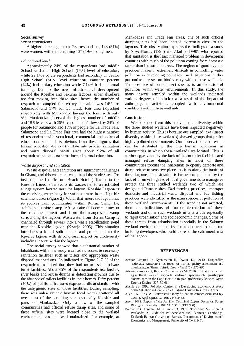
BONOROWO WETLANDS 8 (1): 33-41, June 2018
40
Social survey
Sex of respondents
A higher percentage of the 280 respondents, 143 (51%)
were women, with the remaining 137 (49%) being men.
Educational level
Approximately 24% of the respondents had middle
School or Junior High School (JHS) level of education,
while 22.14% of the respondents had secondary or Senior
High School (SHS) level education. Fourteen percent
(14%) had tertiary education while 7.14% had no formal
training. Due to the new infrastructural development
around the Kpeshie and Sakumo lagoons, urban dwellers
are fast moving into these sites, hence, the number of
respondents sampled for tertiary education was 14% for
Sakumono and 17% for La Trade Fair area (Kpeshie)
respectively with Mankoadze having the least with only
9%. Mankoadze observed the highest number of middle
and JHS leavers with 25% respondents followed by 24% of
people for Sakumono and 18% of people for La Trade Fair.
Sakumono and La Trade Fair area had the highest number
of respondents with vocational, commercial and technical
educational status. It is obvious from these figures that
formal education did not translate into prudent sanitation
and waste disposal habits since about 97% of all
respondents had at least some form of formal education.
Waste disposal and sanitation
Waste disposal and sanitation are significant challenges
in Ghana, and this was manifested in all the study sites. For
instance, the La Pleasure Beach Hotel (adjacent to the
Kpeshie Lagoon) transports its wastewater to an activated
sludge system located near the lagoon. Kpeshie Lagoon is
the receiving water body for various drains in the Kpeshie
catchment area (Figure 2). Water that enters the lagoon has
its sources from communities within Burma Camp, La,
Tebibiano, Teshie Camp, Africa Lake (all communities in
the catchment area) and from the mangrove swamp
surrounding the lagoon. Wastewater from Burma Camp is
channeled through sewers into a waste stabilization pond
near the Kpeshie lagoon (Kpanja 2006). This situation
introduces a lot of solid matter and pollutants into the
Kpeshie lagoon with its long-term impact on biodiversity
including insects within the lagoon.
The social survey showed that a substantial number of
inhabitants within the study area had no access to necessary
sanitation facilities such as toilets and appropriate waste
disposal mechanisms. As indicated in Figure 2, 71% of the
respondents admitted that they had no access to private
toilet facilities. About 45% of the respondents use bushes,
river banks and refuse dumps as defecating grounds due to
the absence of toilets facilities in their homes. Fifty percent
(50%) of public toilet users expressed dissatisfaction with
the unhygienic state of those facilities. During sampling,
there was indiscriminate human fecal matter scattered all
over most of the sampling sites especially Kpeshie and
parts of Mankoadze. Only a few of the sampled
communities had official refuse dump sites, and some of
these official sites were located close to the wetland
environments and not well maintained. For example, at
Mankoadze and Trade Fair areas, one of such official
dumping sites had been located extremely close to the
lagoons. This observation supports the findings of a study
by Noye-Nortey (1990) and Akuffo (1998), who reported
that sanitation is the least managed problem in developing
countries with much of the pollution coming from domestic
rather than industrial sources. The neglect of good hygiene
practices makes it extremely difficult in controlling water
pollution in developing countries. Such situations further
put undue stresses on biodiversity within these wetlands.
The presence of some insect species is an indicator of
pollution within water environments. In this study, the
many insects sampled within the wetlands indicated
various degrees of pollution as a result of the impact of
anthropogenic activities, coupled with environmental
conditions within these wetlands.
Conclusion
We conclude from this study that biodiversity within
the three studied wetlands have been impacted negatively
by human activity. This is because our sampled taxa (insect
diversity within these wetlands) showed groups that prefer
highly polluted environments. Our observations and results
can be attributed to the dire human conditions in
communities in which these wetlands are located. This is
further aggravated by the lack of decent toilet facilities and
managed refuse damping sites in most of these
communities forcing the inhabitants to openly defecate and
dump refuse in sensitive places such as along the banks of
these lagoons. This situation is further compounded by the
lack of or unwillingness of local governments to manage or
protect the three studied wetlands two of which are
designated Ramsar sites. Bad farming practices, improper
domestic and industrial waste disposal and bad fishing
practices were identified as the main sources of pollution of
these wetland environments. If the trend is not arrested,
there are indications of further destruction of these
wetlands and other such wetlands in Ghana due especially
to rapid urbanisation and socioeconomic changes. Some of
these threats from urbanisation especially in the Sakumo
wetland environment and its catchment area come from
building developers who build close to the catchment area
of the lagoon.
REFERENCES
Acquah-Lamptey D, Kyerematen R, Owusu EO. 2013. Dragonflies
(Odonata: Anisoptera) as tools for habitat quality assessment and monitoring in Ghana. J Agric Biodiv Res 2 (8): 178-183.
Adu-Acheampong S, Bazelet CS, Samways MJ 2016.. Extent to which an
agricultural mosaic supports endemic species-rich grasshopper assemblages in the Cape Floristic Region biodiversity hotspot. Agric
Ecosyst Environ 227: 52-60.
Akuffo SB. 1998. Pollution Control in a Developing Economy. A Study of the Situation in Ghana. 2nd ed.. Ghana Universities Press, Accra.
Allan RK. 1973. Willstatter-stoll theory of leaf reflectance evaluated ray tracing. Appl Optics 12 (10): 2448-2453.
Anon. 2001. Report of the Ad Hoc Technical Expert Group on Forest
Biological Diversity (UNEP/CBD/SBSTTA/7/6).
Barbier EB, Acreman M, Knowler D. 1997. "Economic Valuation of
Wetlands: A Guide for Policymakers and Planners," Cambridge,
England: Ramsar Convention Bureau, Department of Environmental Economics and Management, University of York, NY.

MENSAH et al.-Influence of human activities on wetlands diversity
41
Barbour MG, Burk JH, Pitts WD, Gilliam FS, Schwartz MW. 1998.
Terrestrial Plant Ecology. 3rd ed. Addison Wesley Longman, CA.
Benton TG. 1995. Biodiversity and biogeography of Henderson Island insects. Biol J Linn Soc 56(1-2): 245-259.
Biney C. 1995a. The threat of pollution to the coastal zone of the Greater
Accra Metropolitan Area, Ghana. J Sci 47(5): 31-36. Boorman J. 1981. West Africa Insects. Longman Group Limited, UK.
Carter D, Edmonds A, Dewhurst H, Hewson, Bradley JD, Webber C,
Optler A. 1992. Butterflies and Moths. Stoddart Publishing Co. Ltd., Ontario.
Chang L, Kun L, You C, Jongyu S. 2007. Foraging behaviour of three
insect pollinators of Jatropha curcas. www.scielo.br/scelo.php?pid. Chao A, Lee SM. 1992. Estimating the number of classes via sample
coverage. J Amer Stat Assoc 87: 210-217.
Chao A.1987. Estimating the population size for capture-recapture data with unequal catchability. Biometrics 43: 783-791.
Collar NJ, Crosby MJ, Stattesfield AJ. 1994. Birds to Watch 2 (The World
List of Threatened Birds). Official Source for Birds on the IUCN Red List. Birdlife International, Cambridge, UK.
Collison RC, Harlan J, Streeter LR. 1995. Pattern Recognition in Biology.
NOVA Publishers. Inc. UK. Constanza R, D'arge R, De Groot R. 1997. The Value of the World's
Ecosystem Services and Natural Capital. Nature Publishing Group,
USA. Books. Pennsylvania State University, USA. Corbet P. 1980. Biology of Odonata. Annual Review of Entomology.
Cornell University, Press Ithaca, NY.
Davies B, Day JJ. 1998. Vanishing Waters. UCT Press, USA. Deszoley AS, Resh VH. 2000. Factors Influencing Macroinvertebrate
Colonization of Seasonal Wetland: Response to Emergent Plant
Cover. John Wiley & Sons, New York. Gordon I, Cobblah MA. 2000. Insects of the Muni-Pomadze Ramsar Site.
Biodiv Conserv 9 (4): 479-486.
Groombridge B, Jenkins MD. 2002. World Atlas of Biodiversity: Earth's living resources in the 21st century. University of California Press,
Berkeley, CA.
Groves CR. 2002. Drafting a conservation blueprint: A practitioner’s
guide to planning for biodiversity. Island Press, Washington.
Gullan PJ, Cranston PS. 2005. The Insect-An Outline of Entomology. Blackwell, London.
Hynes HBN. 1930. Taxonomy of Aquatic Insects Nymphs and Larvae.
Cambridge University Press, UK. Kpanja D. 2006. The Sub Metro. Annual Report. Govt of Ghana, Accra,
Ghana.
Kwei EA. 1974. Periphyton: Ecology, Exploitation and Management.CABI Publishing, Oxfordshire, UK.
Kyerematen R, Acquah-Lamptey D, Owusu EH, Anderson RS, Ntiamoa-
Baidu Y. 2014. Insect Diversity of the Muni-Pomadze Ramsar Site: An important site for biodiversity conservation in Ghana. J Insects
2014: ID 985684, 11 pages.
Kyerematen R, Adu-Acheampong S, Acquah-Lamptey D, Anderson R. S, Owusu E. H. and Mantey J. 2018. Butterfly diversity: An indicator for
environmental health within the Tarkwa Goldmine, Ghana. Environ
Nat Resour Res 8 (3): 69-83.
Kyerematen R, Kaiwa F, Acquah-Lamptey D, Adu-Acheampong S, Anderson RS. 2018. Butterfly assemblages of two wetlands:
Response of biodiversity to different Environmental stressors in
Sierra Leone. Open J Ecol 8 (7): 1061-1079. Kyerematen R, Owusu EH, Acquah-Lamptey D, Ofori BY, Anderson RS,
Ntiamoa-Baidu Y. 2014. Species composition and diversity of insects
of the Kogyae Strict Nature Reserve in Ghana. Open J Ecol 4: 1061-1079.
May RM, Stumpf MPH. 2000. Estimation of species extinctions. Rain
Forest Conservation Fund, Chicago, IL. Noye-Nortey H. 1990. Effects of pine silviculture on the ant assemblages
(Hymenoptera: Formicidae) of the Patagonian steppe. Elsevier, The
Nederlands. Ntiamoa-Baidu Y, Gordon C. 1991. Coastal wetlands management plans:
Ghana Environmental Resource Manage-ment Project (GERMP)
Report, Ghana Environmental Protection Council and World Bank, Accra.
Ntiamoa-Baidu Y. 1991. Conservation of Coastal Lagoons in Ghana. The
traditional approach. Landsc Urban Plan 20: 41-46. Nummelin M.1996. The community structure of arthropods in virgin and
managed sites in the Kibale Forest, Western Uganda. Trop Ecol 37:
201-213. Oduro W, Aduse-Poku K. 2005. Preliminary assessment of fruit-feeding
butterfly communities in the Owabi wildlife sanctuary. Ghana J For
17: 9-19. Pollard E, Yates TK. 1993. Monitoring butterflies for ecology and
conservation: The British butterfly monitoring scheme. Chapman and
Hall, London. Resh V, Carde R. 2003. Encyclopedia of Insects. Academic Press, San
Diego, CA.
Ryan JM, Attuquayefio DK. 2000. Mammal fauna of the Muni-Pomadze Ramsar site, Ghana. Biodiv Conserv 9: 541-560.
Ryan RO. 2005. Archives of Insect Biochemistry and Physiology. John
Wiley and Sons Inc, New York.
Samways MJ, McGeoch MA, New T. 2010. Insect conservation: a
handbook of approaches and methods. Oxford University Press, UK. Scheren PAGM, Zanting HA, Lemmens AMC. 2000. Estimation of water
pollution sources in Lake Victoria, East Africa: Application and
elaboration of the rapid assessment methodology. J Environ Manag 58 (4): 235-248.
Scholtz JC, Holm RT. 2005. Climate Change Impact: Insects. Dartmouth
College. New Hampshire, US. Seyam IM, Hoekstra AY, Ngabirano GS, Saverije HHG. 2001. The value
of water. Research Report Series No 7. DA Delft, The Netherlands.
Shannon CE, Wiener W. 1949. The mathematical theory of communication.University of Illinois Press, Urbana, IL.
Struhsaker TT. 1998. A biologist’s perspective on the role of sustainable
harvest in conservation. Conserv Biol 12 (4): 930-932. Wilson EO. 1992. Fluctuations in abundance of tropical insects. Harvard
University Press, Cambridge, MA.

BONOROWO WETLANDS P-ISSN: 2088-110X Volume 8, Number 1, June 2018 E-ISSN: 2088-2475
Pages: 42-50 DOI: 10.13057/bonorowo/w080105
Identification and characterization of Flavobacteriaceae from farmed
Oreochromis niloticus and Clarius gariepinus in Uganda
AMONO RACHEAL1, CHRISTOPHER J. KASANGA1,♥, DENIS K. BYARUGABA2 1College of Veterinary Medicine and Biomedical Sciences, Sokoine University of Agriculture. Tanzania. ♥email: [email protected],
[email protected] 2College of Veterinary Medicine, Animal Resource and Biosecurity, Makerere University. Kampala, Uganda
Manuscript received: xxx 2017. Revision accepted: xxx 2018.
Abstract. Racheal A, Kasanga CJ, Byarugaba DK. 2018. Identification and characterization of Flavobacteriaceae from farmed
Oreochromis niloticusand Clarius garieoinus. Bonorowo Wetlands 2: 42-50. Bacteria under family Flavobacteriaceae (in this study were
also referred to as Flavobacteria) are important pathogens of fish, people, many other animals and plants. In this study, Flavobacteria
from Nile tilapia (Oreochromis niloticus) and African catfish (Clarius gariepinus) were identified and characterized from the selected
farms in Uganda. Gill and skin swabs were obtained from a total of 119 fish from 19 farms and were dissected aseptically to sample
internal organs. The samples were inoculated onto Sheih media and incubated at 25°C for 48 hours. The suspected isolates were
identified by colon characteristics, conventional biochemical tests and API 20 NE kits. The isolates were grouped into eight based on
colon characteristic similarity. One isolate was selected per group for 16S rRNA gene sequencing and identified using the
EZbiocloud.net ID software. Phylogenetic analysis of selected isolates was performed using the 16S rRNA gene sequences in BioEdit
and MEGA 7.0.2 software. Basing on extrapolation of sequence analysis of the selected isolates, out of the 86 isolates, Myroides
marinus was the most predominant species taking up 4 of the 8 groups (60 isolates) in 13 farms. The rest of the groups comprised of;
Acinetobacter pitti, one group (6 isolates) in 6 farms, Chryseobacterium gambrini 2 groups (3 isolates) in 3 farms and one isolate was
unidentified, in 3 farms. However, a total of 16 isolates did not grow on sub culturing. Phylogenetic analysis indicated that M. marinus
isolates grouped with other M. marinus isolates from gene bank with significant intra-species diversity which was also observed with C.
gambrini isolates. All the sampled farms had at least one isolate of a Flavobacterium from Tilapia and/or Catfish. Pathogenicity studies
should be conducted on the isolates to establish their importance as fish pathogens and transmission dynamics so that an appropriate
control measure can be recommended.
Keywords: Clarius garieoinus, Flavobacteriaceae, Oreochromis niloticus
INTRODUCTION
Agriculture is the backbone of Uganda`s economy with
aquaculture as one of the major enterprises highly growing,
yet still with enormous potential for production (NDP11
2015/2016-2019/20). However, increase in aquaculture is
accompanied with an increased risk of diseases. Earlier it
was observed during a research that over 70% of fish farms
in central and western Uganda sampled with farmed tilapia
and catfish had a high incidence of four bacterial pathogens
including Pseudomonus sp., Aeromonas sp., Vibrio sp. and
F. columnare of family Flavobacteriaceae (Walakira et al. 2014).
All over the world, there are numerous species of
Flavobacteriaceae having the ruinous affect on the wild as
well as on farmed fish stocks. Flavobacterial disease
eruptions are infamously challenging to avert and control
even though a lot of research has been carried out for
nearly 100 years. They are known for their great economic
and ecological effects (Wagner et al. 2002; Welker et al.
2005). Fish that recover from some Flavobacterial diseases
remain carriers and shed the bacteria into the environment
which makes them more dangerous in aquaculture (Welker
et al. 2005).
Phylogenetic analysis of Flavobacterial fish pathogens
is critical for the appropriate control of infections caused
especially given the fact that Uganda is having a high
growth rate in aquaculture (MAAIF 2004). Information
about the occurrence of Flavobacterial diseases in Uganda
is not well documented but there are several undocumented
cases (unpublished, NAFIRI, Kajansi). The occurrence of
diseases caused by Flavobacterial pathogens in countries
with high aquaculture production like America, Europe and
Asia (Shotts and Starliper 1999; Farmer 2004; Zamora et
al. 2012a,b; Loch and Fasial 2014), could be one of the
indications that Uganda will at one time face the same
problem. It is therefore important to proactively study the
occurrence of species prevalent in the country and with
further studies on their pathogenicity. It may be possible to
develop and implement appropriate control measures such
as vaccination using tailored vaccines.
Specific objectives are to determine the occurrence of
Flavobacteriaceae in Oreochromis niloticus and Clarius
gariepinus in the selected farms in Uganda and to determine
the molecular characteristics of Flavobacteriaceae isolates
from Oreochromis niloticus and Clarius gariepinus in the
selected farms in Uganda, using the 16S rRNA gene.

RACHEAL et al. – Flavobacteriaceae from Oreochromis niloticus and Clarius gariepinus
43
MATERIAL AND METHODS
The study area
The study was conducted on selected farms in the
districts of Wakiso, Kampala, Lira, Arua, Nebbi and Kole
(Kole is a new district that has just been formed from Lira
district) (Figure 1).
Study design
This was a cross sectional study to isolate and identify
Flavobacteriaceae isolates from African catfish and Nile
tilapia in selected farms in Uganda. Bacteria were isolated
from fish collected between October 2016 and March 2017.
These were identified as Flavobacteria basing on growth
colony characteristics (color, elevation, margin texture,
colony consistency), biochemical tests and sequencing of
the 16S rRNA gene.
Sampling
Convenience and purposive sampling techniques were
used in this study. Purposive sampling was done based on
disease history, presence of disease, availability of farms
and accessibility to the farms. A total of 119 fish were
collected from 19 farms. Live fish in water troughs were
transported to the College of Veterinary Medicine Animal
Resources and Biosecurity (COVAB) Central Diagnostic
Laboratory (CDL), Makerere University, Kampala.
Isolation of bacteria under family Flavobacteriaceae
Samples of internal organs were taken aseptically
including kidneys, liver, spleen and these were
homogenized by cutting into smaller pieces using sterile
surgical blade and then inoculated into sheih broth. Swabs
were also obtained from skin, lesions and gills using a
sterile swab stick and inoculated on Shieh`s agar. The
samples were incubated at 25 for 48 hours. Liver, kidney
and spleen were pooled into Shieh broth for 24 hours
before culturing on Shieh agar supplemented with
tobramycin at a concentration of 0.001g/L.
Morphological identification of Flavobacteria colonies
The phenotypic characterization of the isolates was
designed on the basis of colony morphology, Gram staining
and standard biochemical tests along with their
consistency. All yellow bacterial colonies were considered
for the study. Shieh agar and Shieh broth were made for the
bacterial growth as in the table in the appendix 1. Cellular
morphology was determined by Gram staining and viewed
under a microscope whereby gram-negative rods were
considered (magnification, x 100).
Identification of Flavobacteria by biochemical tests
Colonies were grown in peptone water for 48 hours and
motility was determined under light microscope
(magnification, x 100). Other biochemical tests included;
presence of flexirubin type pigments using 1% KOH,
cytochrome oxidase, catalase, TSI (Triple Sugar Iron Agar)
tests (Sebastião et al. 2010). API 20NE test kits from
Biomerieurix were also used both at Makerere University
and Norwegian University of Life Sciences (NMBU) as
screening tests to further identify some isolates before
sequencing.
Figure 1. Map of Uganda and study area
Molecular identification of Flavobacteria
The isolates were preserved on Sheih agar slants and
transported at room temperature to the microbiology
laboratory at the Norwegian University of Life Sciences.
The bacteria were sub-cultured on agar (BHI agar media
was used from DIFCO Laboratories, and Merck KGaA
Germany and the suspected Flavobacteriaceae colonies
were divided into eight groups basing on colony
morphology similarity (basing on colony color, size,
elevation, margin) and one colony per group was selected
for sequencing.
DNA extraction for Flavobacteria sequencing
Genomic DNA was extracted from the 8 selected
isolates at the Gen-lab NMBU where further molecular
analysis was performed. Genomic DNA isolation was done
using QIAamp DNA mini kit (Qiagen). The manufacturer`s
protocol was followed as stated in the appendix 2 and all
spin steps used a bench top Minispin centrifuge.
PCR process for the extracted DNA
The 16S rRNA genes were amplified by PCR using
universal bacteria primers 27f
(5'AGAGTTTGATCCTGGCTCAG-3 and 1492R (5'-
GGTTACCTTGTTACGACTT-3'). Each PCR reaction was
performed in a final volume of 25µL containing: 2.5µL of
10X reaction buffer (50MM, 75MM Tris-HCL pH 9.0),
2MM MgCl2, 20MM (NH4)2SO4), 0.5 µL. 10MM
deoxyribonucleotide mix, 0.2 µL of DNA template, and
16.8 µL of sterile ultrapure water. PCR reactions were
performed by icycler (from BIO-Rad) under the following
conditions: Initial denaturation at 94 °C for 3 mins,

BONOROWO WETLANDS 8 (1): 42-50, June 2018
44
followed by 30 cycles of amplification as follows;
denaturation at 94°C for 30s, annealing at 56°C for 30s and
extension at 72°C for 2 mins, followed by a final extension
step at 72°C for 5 minutes and left to stand at 4°C until
analysis.
Electrophoresis
The PCR products were then run on 1% ultra-pure
agarose (Invitrogen, Thermo Fisher Scientific) using Power
Pac 300 (BioRad) at 100Volts for 60 minutes with Gene
RulerTM 1 kb Ladder. The gels prestained with syberSafe
(source) were visualized using Safe ImagerTM (Invitrogen)
and bands of interest excised with a scalpel blade. Gel
pictures were captured using ChemiDocTM XRS Molecular
imager (Bio Rad).
Purification of the PCR products and sequencing
The PCR products were purified using QIAquick Gel
extraction kit (Quiagen) following manufacturer’s
instructions as stated in appendix 2. The Purified PCR were
quantified, and quality checked using Nanodrop ND-1000
Spectrophotometer (Thermo Fisher Scientific inc.) and sent
for sequencing by sanger sequencing technology and
technique at GATC Biotech, Germany using the same
primers as those used for PCR.
Data analysis
Data was summarized and stored in Microsoft excel
version 10. BLAST searches were done online to get
similar sequences from the gene banks using NCBI
website. The obtained sequences from isolates in this study
were edited using bioedit and aligned with those retrieved
from gene banks using Claustal W algorithm in MEGA
version 7.0 software. The alignments were used to
construct phylogenetic tree using Neighbor Joining method
using Kimura-2-parameter model. Identification of the
sequences was also done using EZBiocloud.net ID software
online.
RESULTS AND DISCUSSION
Biodata for the sampled farms
Data of the sampled farms can be seen in Table 1.
Symptoms encountered in the fish samples
Both symptomatic and asymptomatic fish were sampled
and some of the lesions encountered in the symptomatic
fish included: hemorrhages on skin, fins, barbells, yellow
skin, skin erosions, swollen belly, eroded tail fin, pale liver.
Figure 2 shows some of the lesions.
Table 1. Biodata of the selected farms
Status of farmer No. of units Species of fish Sources of water History of disease Culture systems
16 small scale farms 2-5 units for
small scale
Koi carp
Silver carp
Lake
River
Underground
Streams
5 farms (26.31%)
with disease
outbreak/ history
13 farms with only earthen
ponds
3 farms with only cages
3 large scale farms over 20 units for
large scale
African catfish
Tilapia
2 farms with tanks and ponds
1 farm with tanks only
Figure 2. Lesions encountered on catfish
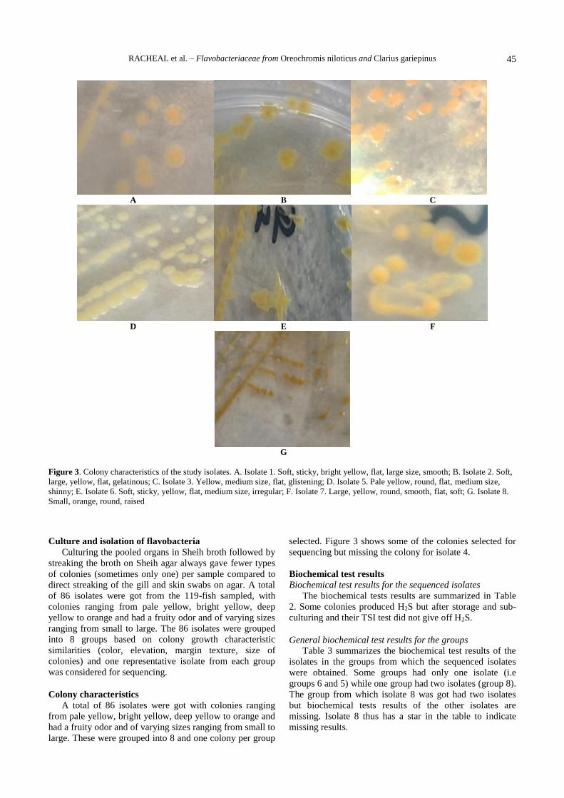
RACHEAL et al. – Flavobacteriaceae from Oreochromis niloticus and Clarius gariepinus
45
A B C
D E F
G
Figure 3. Colony characteristics of the study isolates. A. Isolate 1. Soft, sticky, bright yellow, flat, large size, smooth; B. Isolate 2. Soft,
large, yellow, flat, gelatinous; C. Isolate 3. Yellow, medium size, flat, glistening; D. Isolate 5. Pale yellow, round, flat, medium size,
shinny; E. Isolate 6. Soft, sticky, yellow, flat, medium size, irregular; F. Isolate 7. Large, yellow, round, smooth, flat, soft; G. Isolate 8.
Small, orange, round, raised
Culture and isolation of flavobacteria
Culturing the pooled organs in Sheih broth followed by
streaking the broth on Sheih agar always gave fewer types
of colonies (sometimes only one) per sample compared to
direct streaking of the gill and skin swabs on agar. A total
of 86 isolates were got from the 119-fish sampled, with
colonies ranging from pale yellow, bright yellow, deep
yellow to orange and had a fruity odor and of varying sizes
ranging from small to large. The 86 isolates were grouped
into 8 groups based on colony growth characteristic
similarities (color, elevation, margin texture, size of
colonies) and one representative isolate from each group
was considered for sequencing.
Colony characteristics
A total of 86 isolates were got with colonies ranging
from pale yellow, bright yellow, deep yellow to orange and
had a fruity odor and of varying sizes ranging from small to
large. These were grouped into 8 and one colony per group
selected. Figure 3 shows some of the colonies selected for
sequencing but missing the colony for isolate 4.
Biochemical test results
Biochemical test results for the sequenced isolates
The biochemical tests results are summarized in Table
2. Some colonies produced H2S but after storage and sub-
culturing and their TSI test did not give off H2S.
General biochemical test results for the groups
Table 3 summarizes the biochemical test results of the
isolates in the groups from which the sequenced isolates
were obtained. Some groups had only one isolate (i.e
groups 6 and 5) while one group had two isolates (group 8).
The group from which isolate 8 was got had two isolates
but biochemical tests results of the other isolates are
missing. Isolate 8 thus has a star in the table to indicate
missing results.

BONOROWO WETLANDS 8 (1): 42-50, June 2018
46
API test results
The API test results shown in the Table 4 were for some
selected isolates most of which were not sequenced directly
or did not regrow on sub culturing thus. Some isolates
tested using the API 20NE kits gave codes which had
unacceptable profiles and therefore were not identified as
shown in Table 4.
Table 2. Biochemical test results of the sequenced isolates
Iso
late
Ca
tala
se
Ox
ida
se
Fle
xir
ub
in P
igm
ent
Co
ngo
red
ab
sorp
tio
n
H2S
Ure
ase
Gel
ati
na
se
Ind
ole
pro
du
ctio
Mo
tili
ty
Glu
cose
fer
men
tati
Ga
s o
ff g
luco
se
Su
cro
se f
erm
enta
ti
1 + + + + - + - + - - - +
2 + + + + - + + - - - - -
3 + + + + - + + - - - - -
4 + + + + - - + - - - - -
5 + + + + - - - - - - - -
6 + + + + - - + - + - - -
7 - + + + - + - - - - - -
8 + + + + - - + - - + + -
Table 4. API 20NE results
Isolate Group Identification Percentage
Identification
A NR Unacceptable profile N/A
B NR Unacceptable profile N/A
C NR Unacceptable profile N/A
D NR C. indolgenes 90.6
E NR Acinetobacter sp. 60
F NR C. indolgenes 99.9
G 1 Myroides sp. 64
H 1 Weeksiela sp. 37
1 1 Myroides sp. 64
I 3 C. indolgenes 49
Note: NR- Not represented in the groupings since did not grow on
sub-culturing N/A- Not applicable
Comparison of conventional and API 20NE biochemical
test results
The biochemical tests compared between the
conventional laboratory method and the API 20NE kits
were glucose fermentation, presences of urease activity
(URE), gelatin hydrolysis (GEL) by gelatinase, oxidase
activity (OX) and indole production (TRP). There were
minimal differences in the test results observed between the
two methods (not more than two tests out of the five tests
per isolate) as observed in the Table 5.
Electrophoresis results
Figure 4 shows the electrophoresis results with the
bands of sizes of approximately 1500bp (indicated by an
arrow) obtained using universal bacterial primers 27F and
1492R.
Table 5. Comparison of API 20NE and conventional tube test
results for selected isolates
Isolate Test method GLU URE GEL OX TRP
A API - + + + +
Conventional - - + + +
B API + - + + +
Conventional - + + + +
3 API - + + + -
Conventional missing + + + -
C API - - + + +
Conventional - - - + +
D API - - + - +
Conventional - - + + +
E API - + + - -
Conventional - + missing + +
F API - + + - +
Conventional - + + + +
1 API - + + - -
Conventional - + + + +
G API - + + - -
Conventional - + + + -
H API - - + - -
Conventional - + + + -
I API - + + - -
Conventional - + + + -
Table 3. General biochemical test results of the groups
Representative sequenced
isolate
1 2 3 4 5 6 8*
No. of isolates in the group 14 3 30 13 1 1 2
Flexirubin 92.9 (+) 100 (+) 93.3 (+) 76.2 (+) (+) (+) (+)
Catalase 100 (+) 100 (+) 96.7 (+) 100 (+) (+) (+) (+)
Oxidase 85.7 (+) 66.7 (-) 86.7 (+) 70.0 (+) (+) (+) (+)
Congo red 100 (+) 100 (+) 93.3 (+) 70.0 (+) (+) (+) (+)
Urease 100 (+) 100 (+) 60.0 (+) 76.9 (+) (-) (-) (-)
TSI 92.9 (-) 100 (-) 83.3 (-) 84.6 (-) (-) (-) (+)
H2S 100 (-) 100 (-) 96.7 (+) 100 (-) (-) (-) (-)
Gliding motility 92.9 (-) 66.7 (-) 93.3 (-) 84.6 (-) (+) (-) (-)
Indole production 71.4 (-) 100 (-) 70.0 (-) 53.8 (-) (-) (-) (-)
Gelatin hydrolysis 50.0 (+) 100 (+) 73.3 (+) 92.3 (+) (+) (+) (+)
Glucose fermentation 92.9 (-) 100 (-) 96.7 (-) 92.3 (-) (-) (-) (+)
Gas from glucose fermentation 100 (-) 100 (-) 100 (-) 92.3 (-) (-) (-) (+)
Sucrose fermentation 92.9 (-) 100 (-) 93.3 (-) 92.3 (-) (-) (-) (-)

RACHEAL et al. – Flavobacteriaceae from Oreochromis niloticus and Clarius gariepinus
47
Figure 4. Electrophoresis results for the 16S rRNA gene
Identification and occurrence of the isolates
Identification of isolates using Ezbiocloud.net
The commonest species that was isolated was M.
marinus and the closest strain to the isolates was M.
marinus JS 08 (GQ857652) at a percentage similarity of
99.0 to 99.79% (for the different group isolates) using
Ezbioclod.net. These were isolated on 15 farms out of the
19 sampled farms. The least common species isolated were
those closely similar to M. odoramitimus, with closet strain
as M. odoratimimus CCUG 39352 at percentage similarity
of 86.7% and Chryseobacterium gambrini with closest
strain as C. gambrini DSM 18014 at a percentage similarity
of 98.37 to 97.82% (for the different selected isolates)
using Ezbiocloud.net.
Table 6 shows the identification of the isolates, the
health status, species of fish (Oreochromis niloticus (O.n)
or Clariaus gariepinus (C.g) and site of fish from which
they were isolated, culture system and water source of the
farms from which the isolates were obtained.
Identification of the 86 isolates
Figure 5 shows the composition of the isolates based on
extrapolation of the results of the sequenced isolates.
Phylogenetic analysis
Occurrence of flavobacteria on the farms
Out of the 19 sampled farms, Myroides marinus was the
commonest while the unidentified isolate was the least
common. The isolates were distributed on the farms as
summarized in Figure 6.
Key: Neighbor-Joining method was used to imply the
evolutionary history (Saitou and Nei 1987). in which the
sum of branch length = 0.51734957 was shown by optimal
tree. The percentage of replicate trees in which the
associated taxa clustered together in the bootstrap test
(1000 replicates) are shown next to the branches
(Felsenstein 1985). The evolutionary distances were
computed using the Kimura 2-parameter method (Kimura
1980) and are in the units of the number of base
substitutions per site. The analysis involved 16 nucleotide
sequences. All positions containing gaps and missing data
were eliminated. There was a total of 989 positions in the
final dataset. Evolutionary analyses were conducted in
MEGA7 (Kumar et al. 2016).
The isolates 1,2,3 and 4 were grouped with the other M.
marinus isolates obtained from the gene bank. Isolate 2 and
3 were more closely related to each other and to the
reference strain M. marinus JS 08 compared to isolate 1
and 4. Isolate 4 was furthest from the reference strain of all
the M. marinus isolates. Therefore, there is diversity in the
phylogenetic relatedness between the isolates 1,2,3 and 4.
Isolate 6 did not cluster with any of the other isolates.
Isolates 8 and 5 were grouped with the other C. ganbrini
isolates obtained from the gene bank. Isolate 5 was more
closely related to the reference strain compared to isolate 8.
Table 6. Identification of isolates and their occurrence in fish
Iso
late
Sta
tus
of
fish
Per
cen
tag
e
sim
ila
rity
an
d C
lose
st
stra
in u
sin
g
EZ
Bio
clo
ud
.n
Sp
ecie
s o
f fi
sh
Sit
e o
n s
am
ple
d
fish
Cu
ltu
re S
yst
em
Wa
ter
sou
rce
1 Symptomatic and
symptomatic
Myroides marinus
JS 08 (99.49%)
Cg Pooled liver, spleen, gills Tank, pond Rain, tap water
2 Assympt- omatic Myroides marinus
JS 08 (99.79%)
Cg, O.n Gills and skin Pond Stream
3 Assympt- omatic Myroides marinus
JS 08 (99.0%)
Cg,
O.n
Pooled kidney, liver,
spleen, skin gills
Pond Stream
4 Assympt- omatic fish Myroides marinus
JS 08 (99.79%)
Cg Pooled organs, liver,
spleen, kidney
Pond, tank Lake
5 Symptomatic fish Chryseobacterium gambrini
DSM 18014 (98.37%)
O.n Pooled organs,
skin, gills
Pond Stream
6 Assympt- omatic Myroides odoratimimus
CCUG39352 (86.7%)
O.n Pooled organs, liver,
spleen kidney
Pond, Tank Lake
7 Symptom- atic fish Acinetobacter pittii
CIP 70.29 (99.36%)
O.n Gills, skin Pond, cage Lake
8 Symptomatic and
symptomatic
Chryseobacterium gambrini
DSM 18014 (98.19%)
Cg,
O.n
Pooled organs, liver,
spleen kidney
Tank Tap water, rain
water
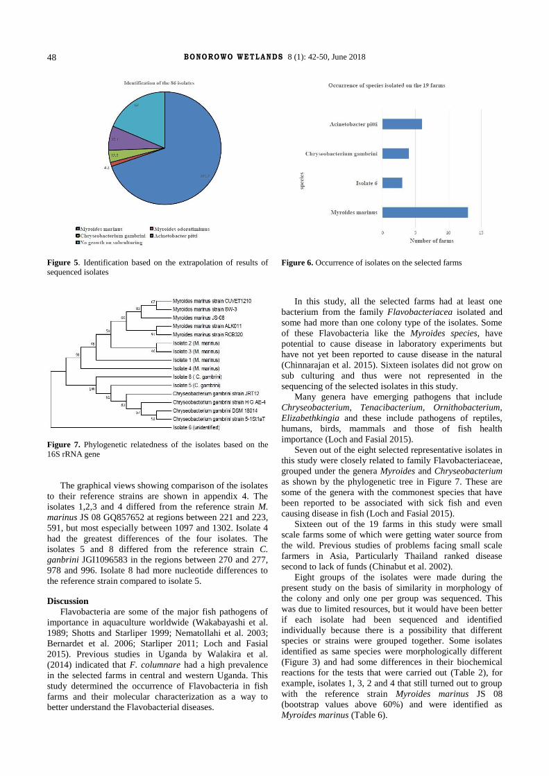
BONOROWO WETLANDS 8 (1): 42-50, June 2018
48
Figure 5. Identification based on the extrapolation of results of
sequenced isolates
Figure 6. Occurrence of isolates on the selected farms
Figure 7. Phylogenetic relatedness of the isolates based on the
16S rRNA gene
The graphical views showing comparison of the isolates
to their reference strains are shown in appendix 4. The
isolates 1,2,3 and 4 differed from the reference strain M.
marinus JS 08 GQ857652 at regions between 221 and 223,
591, but most especially between 1097 and 1302. Isolate 4
had the greatest differences of the four isolates. The
isolates 5 and 8 differed from the reference strain C.
ganbrini JGI1096583 in the regions between 270 and 277,
978 and 996. Isolate 8 had more nucleotide differences to
the reference strain compared to isolate 5.
Discussion
Flavobacteria are some of the major fish pathogens of
importance in aquaculture worldwide (Wakabayashi et al.
1989; Shotts and Starliper 1999; Nematollahi et al. 2003;
Bernardet et al. 2006; Starliper 2011; Loch and Fasial
2015). Previous studies in Uganda by Walakira et al.
(2014) indicated that F. columnare had a high prevalence
in the selected farms in central and western Uganda. This
study determined the occurrence of Flavobacteria in fish
farms and their molecular characterization as a way to
better understand the Flavobacterial diseases.
In this study, all the selected farms had at least one
bacterium from the family Flavobacteriacea isolated and
some had more than one colony type of the isolates. Some
of these Flavobacteria like the Myroides species, have
potential to cause disease in laboratory experiments but
have not yet been reported to cause disease in the natural
(Chinnarajan et al. 2015). Sixteen isolates did not grow on
sub culturing and thus were not represented in the
sequencing of the selected isolates in this study.
Many genera have emerging pathogens that include
Chryseobacterium, Tenacibacterium, Ornithobacterium,
Elizabethkingia and these include pathogens of reptiles,
humans, birds, mammals and those of fish health
importance (Loch and Fasial 2015).
Seven out of the eight selected representative isolates in
this study were closely related to family Flavobacteriaceae,
grouped under the genera Myroides and Chryseobacterium
as shown by the phylogenetic tree in Figure 7. These are
some of the genera with the commonest species that have
been reported to be associated with sick fish and even
causing disease in fish (Loch and Fasial 2015).
Sixteen out of the 19 farms in this study were small
scale farms some of which were getting water source from
the wild. Previous studies of problems facing small scale
farmers in Asia, Particularly Thailand ranked disease
second to lack of funds (Chinabut et al. 2002).
Eight groups of the isolates were made during the
present study on the basis of similarity in morphology of
the colony and only one per group was sequenced. This
was due to limited resources, but it would have been better
if each isolate had been sequenced and identified
individually because there is a possibility that different
species or strains were grouped together. Some isolates
identified as same species were morphologically different
(Figure 3) and had some differences in their biochemical
reactions for the tests that were carried out (Table 2), for
example, isolates 1, 3, 2 and 4 that still turned out to group
with the reference strain Myroides marinus JS 08
(bootstrap values above 60%) and were identified as
Myroides marinus (Table 6).

RACHEAL et al. – Flavobacteriaceae from Oreochromis niloticus and Clarius gariepinus
49
The colony morphological and biochemical differences
could be due to differences in the strains which was not
well studied here. The fact that some of the isolates had
phylogenetic relationship and yet were found in different
farms in different parts of the country, could be an
indication of similar source. Most of the sampled farms had
previously received fingerlings from Kajansi through a
government project to support fish farmers in Uganda, thus
could be a common source. Isolate 6 was not closely
related to any of the other isolates in this study, not even to
M. odoratimimus which was the closest possible species.
Although the closest strain was M. Odoratimimus, the
percentage similarity of 86.7% is low and thus the isolate is
a bacterium probably not under family Flavobacteriaceae.
Isolate 7 although with colony and biochemical
characteristics similar to Flavobacteria, was identified as
Acinetobacter pitti using EZtaxon ID software. The
biochemical tests of many colonies in this study tentatively
suggested F. columnare but were ruled out by the API kits
and 16S rRNA gene sequencing. There were differences in
the biochemical characteristics of isolates between and
within the groups formed as shown in Tables 3 and 4. This
could be because of differences in species or strains among
the isolates in each group. The colony characteristics
(color, size, elevation colony margins) similarity used to
group the isolates is not sufficient to differentiate the
bacteria species or strains of Flavobacteria. For example,
isolates 1, 2 and 3 were all identified as M. marinus but
have different colony growth characteristics as shown in
Figure 3. Graphical views in the appendix 3 revealed
differences in their nucleotides between the isolates 1, 2, 3
and 4 and thus could be due to differences in the strains.
Similarly, isolates 5 and 8 where both identified as C.
gambrini but had differences in biochemical test results for
example isolate 8 fermented glucose, produced acid on TSI
and did not have gliding motility while isolate 5 did not
ferment glucose, no acid production in TSI and had gliding
motility. API 20NE kits when used in this study could rule out F.
columnare even though morphological and biochemical
tests suggested otherwise. The comparison of identification
by API kits and 16s RNA gene sequencing was not well
studied here, although both API kits and 16S RNA gene
sequencing did not identify any of the major Flavobacteria.
The API test results for isolates G and I at 64% identity
gave a correct genus identification even though the
percentage identity was still considered low while for
isolates H and I whose percentage identification were
below average; the identification was not correct compared
to sequence identification. The API results in this study had
generally low percentage identities and were not reliable.
Adley and Saieb (2005) compared biomeriueux API 20NE
and Remel RapiD NF Plus in the identification systems of
type strains of Ralstonia picketti. Only 29 out of 48 isolates
were identified and the API 20NE was considered
inconsistent. However, use of API kits (API NE and API
ZYM) in a study by Farmer proved to be useful in the
identification of F. columnare (Farmer 2004). API NE kits
when used in this study could rule out F. columnare even
though colony morphology on sheih agar and biochemical
tests suggested otherwise. The comparison of identification
by API kits and 16s RNA gene sequencing was not well
studied here, although both API kits and 16S RNA gene
sequencing did not identify any of the major Flavobacteria.
There were minimal differences in the five test results
observed between the two methods (not more than two
tests out of the five tests per isolate) as observed in the
Table 5. However, the number of samples tested, and the
number of the biochemical tests compared were both too
small to be reliable for a consequence.
Distinct findings were furnished in this study as
comparable from those of the previous studies done in
Uganda which have indicated a high incidence of F.
columnare (Walakira et al. 2014). In this study, there is
however a high occurrence of bacteria under family
Flavobacteriaceae with the exception of F. columnare.
There is a possibility that the presumed F. columnare in
Walakira et al. (2014) study could have been different
species under the different genera of family Flavobacteria-
ceae. The physiological, morphological and biochemical
analysis of the suspected F. columnare colonies in that
study probably led to a misdiagnosis. The diagnosis of
lesser - known Flavobacteria in fish is difficult and
laborious (considering F. columnare, F. branchiophilum
and F. psychrophillum as the major Flavobacteria (Loch
and Fasial 2015). This is because there are few diagnostic
reagents specific for the lesser-known fish associated
Flavobacteria organisms. Diagnosis is further made more
difficult by the fact that Flavobacteria are being discovered
at a high rate and their classifications keep on changing
(Bernardet et al. 1996; Qu et al. 2009; Lee et al. 2010,
Yoon et al. 2011; Loch and Fasial 2015). Varga et al.
(2016) similarly conducted a survey for incidence of F.
columnare in wild and cultured freshwater fish species in
Hungary. Total twenty-five isolates from wild and cultured
freshwater fishes were identified as F. columnare by using
specific PCR. However, both the fragment lengths and the
results of PCR-RFLP genotyping with BsuRI (HaeIII) and
RsaI restriction enzymes were not convincing enough
regarding F. columnare classification. Sequencing of the
16S ribosomal RNA gene revealed that 23 isolates
belonged to the species F. johnsoniae and two represented
Chryseobacterium spp. thus showing that misidentification
of Flavobacteria is easily possible (Varga et al. 2016).
The commonest of the Flavobacteria isolated in the
selected farms in this study was M. marinus as indicated in
Table 3 and Figures 2 and 3. The isolates were got from both
symptomatic and asymptomatic fish for example isolates
(Table 6). Clinical signs in the symptomatic fish included
skin erosions, hemorrhages, yellowing of the skin, swollen
belly and fin erosions as shown in Figure 2. Some of the
isolates from symptomatic fish with skin erosions for example
isolates 1 and 8 were recovered from catfish fingerlings
(Clariaus gariepinus) that were reported to be experiencing
abnormal mortalities for a week. The isolate 8 was
identified as C. gambrini. Loch in his study stated that
Flavobacterium sp. and Chryseobacterium spp. were a
extensive cause of fingerling and fry mortalities in Michigan
(Loch 2014). For this case however, it requires further
experimental studies to tell if the isolates were the causative

BONOROWO WETLANDS 8 (1): 42-50, June 2018
50
agents for the skin erosions and death of the catfish
fingerlings since there is a possibility of mixed infection.
A previous study by Loch has shown different
Flavobacteria species being isolated from both
symptomatic (with hemorrhages, skin and fin erosions, gill
necrosis) and asymptomatic fish, some of which were just
emerging fish pathogens (Loch 2014). Other than the three-
main fish disease causing Flavobacteria, other emerging
Flavobacteria have also been found to cause hemorrhages,
erosions on the skin and fins (Loch and Fasial 2015). The
Original Flavobacteria known to be causing fish health
issues were the F. columnare, F. branchiophilum, F.
psychrophilum but there are many other Flavobacteriacea
causing disease in fish. The newly identified Flavobacteria
vary in the degree of virulence for example, C. aahli sp.
Nov., was found to be mildly pathogenic to fish under
laboratory conditions while F. spartani sp. nov., was rather
more pathogenic (Loch 2014). Thus, it is important to
study pathogenicity of emerging Flavobacteria.
Some farmers reported poor growth of fish. This could
be due to many other factors that could include but not
limited to poor management, genetic factors, reproduction
in Tilapia and diseases. However, Flavobacteriosis is one
of the diseases that could lead to poor growth of fish that
survive the infection. Acute Flavobacteriosis was reported
to contribute to poor growth in fish that survive which
sometimes present with spinal abnormalities (Austin and
Austin 2007).
Conclusion
All the sampled farms had at least one isolate of
Flavobacterium from Tilapia and/ or Catfish. Myroides
marinus was common in the selected farms in this study
isolated on 13 farms which is 68.4% of the 19 farms.
However, C. gambrini (on 4 farms) and the unidentified
isolate 6 (on 3 farms) were not very common in the
selected farms. None of the major Flavobacteria (F.
columnare, F. branchiophilum and F. psychrophillum) was
identified in this study. The routinely used biochemical and
morphological growth characteristics were not sufficient to
identify Flavobacteria. Phylogenetic analysis indicated that
M. marinus isolates grouped with other M. marinus isolates
from gene bank although intra-species diversity was observed,
a similar situation observed with C. gambrini isolates.
REFFERENCE
Adley CC, Saieb FM. 2005. Comparison of biomeriueux API 20NE and Remel RapiD NF Plus, identification systems of type strains of
Ralstonia pickettii. Lett Appl Microbiol 41 (2): 136-140.
Austin B, Austin DA. 2007. Bacterial fish pathogens: diseases of farmed and wild fish, 4th ed. Praxis Publishing Ltd, United Kingdom.
Bernardet JF, Hugo C, Bruun B. 2006. The genera Chryseobacterium and
Elizabethkingia the prokaryotes: a handbook on the biology of bacteria, 3rd edition. Springer 638-76.
Bernardet JF, Segers P, Vancanneyt M, Berthe F, Kersters K, Vandamme
P. 1996. Cutting a Gordian knot: Amended classification and description of the genus Flavobacterium, amended description of the
family Flavobacteriaceae and proposal of Flavobacterium hydatis
nom. nov. Int J Syst Bacteriol 46 (1): 128-148. Chinabut S, Somsiri T, Danayadol. 2002. Impacts of disease in small-
scale aquaculture in Thailand: case studies, Primary Aquatic Animal
Health Care in Rural, Small-scale, Aquaculture Development. FAO
Fish Tech Pap 406. Chinnarajan R, Govindaswamy RV, Rajasabapathy R, LogeshwaranV,
Sreepada RA. 2015. Infection and pathogenecity of Myroides
odoratimimus (NIOCR-12) isolated from the gut of grey mullet
(Mugil cephalus Linnaeus, (1758)). J Microbiol 88: 22-28. Farmer B. 2004. Improved methods for the isolation and characterization
of Flavobacterium columnare.[Dissertation]. Louisiana State
University, Agricultural and Mechanical College, Baton Rouge, LA. Felsenstein J. 1985. Confidence limits on phylogenies: An approach using
the bootstrap. Evol 39: 783-791.
Kimura M. 1980. A simple method for estimating evolutionary rate of base substitutions through comparative studies of nucleotide
sequences. J Mol Evol 16: 111-120.
Kumar S, Stecher G, Tamura K. 2016. MEGA7: Molecular Evolutionary Genetics Analysis version 7.0 for bigger datasets. Mol Biol Evol 33:
1870-1874.
Lee SH, Kim JM, Lee JR, Park W, Jean CO. 2010. Flavobacterium fluviin sp. nov., isolated from stream sediment. Int J Sys Evol Microbiol 60
(2): 353-357.
Loch PT, Faisal M. 2015. Emerging Flavobacterial infections in fish: A review. J Adv Res 6 (3): 283-300.
Loch PT. 2014. Identification of novel Flavobacteria from Michigan and
assessment of their impacts on fish health. Michigan State Univ., USA. Loch T, Faisal M. 2014. Chryseobacterium aahli sp. nov., isolated from
lake trout (Salvelinus namaycush) and brown trout (Salmo trutta), and
emended descriptions of Chryseobacterium ginsenosidimutans and Chryseobacterium gregarium. Intl J Syst Evol Microbiolol 64 (5):
1573-1579.
MAAIF [Ministry of Agriculture Animal Industry and Fisheries]. 2004. The National Fisheries Policy. 1st edition. Department of Fishery
Resources. Kampala, Uganda.
Nematollahi A, Decostere A, Pasmans F, Haesebrouck F. 2003. Flavobacterium psychrophilum infections in salmonid fish. J Fish Dis
26 (10): 563-74.
Qu JH, Yuan HL, Li HF, Deng CP. 2009. Flavobacterium Cauense sp.
Nov., isolated from sediment of eutrophic lake. Int J Sys Evol
Microbiol 59 (11): 2666-2669. Saitou N, Nei M. 1987. The Neighbor-Joining Method-a New Method for
Reconstructing Phylogenetic Trees. Mol Biol Evol 4: 406-425.
Sebastião FA, Pilarski F, Lemos MVF. 2010. Isolation and molecular characterization of Flavobacterium columnare strains from fish in
Brazil. J Bacteriol Res 2 (3): 22-29.
Shotts E, Starliper C. 1999. Flavobacterial diseases: columnaris disease, cold- water disease and bacterial gill disease (Fish diseases and
disorders: viral, bacterial and fungal infections). CABI Publishing;
New York (NY) 3: 559- 576. Starliper CE. 2011. Bacterial coldwater disease of fishes caused by
Flavobacterium psychrophilum. J Adv Res 2 (2): 97- 108.
Varga Z, Sellyei B, Paulus P, Papp M, Molnár K, Székely C. 2016. isolation and characterisation of Flavobacteria from wild and cultured
freshwater fish species in Hungary. Acta Vet Hung 64 (1): 13- 25.
Wagner BA, Wise DJ, Khoo LH, Terhune JS. 2002. The epidemiology of bacterial diseases in food-size channel catfish. J Aquat Anim Health
14: 263-272.
Wakabayashi H, Huh G, Kimura N. 1989. Flavobacterium branchiophila sp. nov., a causative agent of bacterial gill disease of freshwater
fishes. Int J Sys Bacteriol 39 (3): 213-216.
Walakira J, Akoll P, Engole M, Sserwadda M, Nkambo M, Namulawa V, Kityo G, Musimbi F, Abaho I, Kasigwa H, Mbabazi D, Kahwa D,
Naigaga I, Birungi D, Rutaisire J, Majalija S. 2014. Common fish
diseases and parasites affecting wild and farmed Tilapia and catfish in Central and Western Uganda. Uganda J Agric Sci 15 (2): 113 - 125.
Welker LT, Shoemaker AC, Arias RC, Klesius HP. 2005. Transmission
and detection of Flavobacterium columnare in channel catfish Ictalurus punctatus. Dis Aquat Org 63 : 129-138.
Yoon JH, Park S, Kang SJ, Myung SC, Kim W. 2011. Flavobacterium
ponti sp. nov., isolated from seawater. Int J Sys Evol Microbiol 61 (1): 81-85.
Zamora L, Fernández-Garayzábal J, Palacios M, Sánchez-Porro C,
Svensson-Stadler L, Domínguez L. 2012. Chryseobacterium oncorhynchi sp. nov., isolated from rainbow trout (Oncorhynchus
mykiss). Syst Appl Microbiol 35 (1): 24-29.
Zamora L, Vela AI, Palacios MA, Sánchez-Porro C, Svensson-Stadler LA, Domínguez L. 2012. Chryseobacterium viscerum sp. nov., isolated
from diseased fish. Int J Syst Evol Microbiol 62 (12): 2934-2940.

GUIDANCE FOR AUTHORS
Aims and Scope Bonorowo Wetlands encourages submission of manuscripts
dealing with all topics relevant to freshwater, brackish and marine coastal
ecosystems, include zoology, botany, ecology, geology, sedimentology,
hydrology, biogeochemistry; waste water disposal; as well as management, laws and regulations, policy and economics.
Article types The journal seeks original full-length research papers, reviews,
and short communication. Manuscript of original research should be written in no more than 8,000 words (including tables and picture), or proportional with
articles in this publication number. Review articles will be accommodated, while,
short communication should be written at least 2,000 words, except for pre-study. Submission The journal only accepts online submission through system or
email to the editors at [email protected] (until the end of 2017). Submitted
manuscripts should be the original works of the author(s). The manuscript must be accompanied by a cover letter containing the article title, the first name and
last name of all the authors, a paragraph describing the claimed novelty of the
findings versus current knowledge. Submission of a manuscript implies that the submitted work has not been published before (except as part of a thesis or
report, or abstract); and is not being considered for publication elsewhere.
When a manuscript written by a group, all authors should read and approve the final version of the submitted manuscript and its revision; and agree the submission
of manuscripts for this journal. All authors should have made substantial
contributions to the concept and design of the research, acquisition of the data and its analysis; drafting of the manuscript and correcting of the revision. All
authors must be responsible for the quality, accuracy, and ethics of the work.
Acceptance The only articles written in English (U.S. English) are accepted for publication. Manuscripts will be reviewed by editors and invited
reviewers (double blind review) according to their disciplines. Authors will
generally be notified of acceptance, rejection, or need for revision within 1 to 2 months of receipt. The manuscript is rejected if the content does not in line with
the journal scope, does not meet the standard quality, inappropriate format,
complicated grammar, dishonesty (i.e. plagiarism, duplicate publications, fabrication of data, citations manipulation, etc.), or ignoring correspondence in
three months. The primary criteria for publication are scientific quality and
biodiversity significance. Uncorrected proofs will be sent to the corresponding author as .doc or .rtf files for checking and correcting of typographical errors. To
avoid delay in publication, corrected proofs should be returned in 7 days. The accepted papers will be published online in a chronological order at any time,
but printed in June and December.
Ethics Author(s) must obedient to the law and/or ethics in treating the object of research and pay attention to the legality of material sources and
intellectual property rights.
Copyright If and when the manuscript is accepted for publication, the author(s) still hold the copyright and retain publishing rights without
restrictions. Authors or others are allowed to multiply article as long as not for
commercial purposes. For the new invention, authors are suggested to manage its patent before published.
Open access The journal is committed to free-open access that does not
charge readers or their institutions for access. Readers are entitled to read, download, copy, distribute, print, search, or link to the full texts of articles, as
long as not for commercial purposes. The license type is CC-BY-NC-SA.
A charge The journal is committed to free of charge for submission and publication of non-institutional funded research (waiver).
Reprints The sample journal reprint is only available by special request.
Additional copies may be purchased when ordering by sending back the uncorrected proofs by email.
Manuscript preparation Manuscript is typed on A4 (210x297 mm2) paper
size, in a single column, single space, 10-point (10 pt) Times New Roman font. The margin text is 3 cm from the top, 2 cm from the bottom, and 1.8 cm
from the left and right. Smaller lettering size can be applied in presenting table
and figure (9 pt). Word processing program or additional software can be used, however, it must be PC compatible and Microsoft Word based (.doc or .rtf; not
.docx). Scientific names of species (incl. subspecies, variety, etc.) should be
written in italic, except for italic sentence. Scientific name (genera, species, author), and cultivar or strain should be mentioned completely for the first time
mentioning it in the body text, especially for taxonomic manuscripts. Name of
genera can be shortened after first mentioning, except generating confusion. Name of the author can be eliminated after first mentioning. For example,
Rhizopus oryzae L. UICC 524, hereinafter can be written as R. oryzae UICC
524. Using trivial name should be avoided, otherwise generating confusion. Biochemical and chemical nomenclature should follow the order of the
IUPAC - IUB. For DNA sequence, it is better used Courier New font. Symbols
of standard chemical and abbreviation of chemistry name can be applied for common and clear used, for example, completely written butilic hydroxyl
toluene (BHT) to be BHT herein after. Metric measurement use IS
denomination, usage other system should follow the value of equivalent with
the denomination of IS first mentioning. Abbreviations set of, like g, mg, mL,
etc. do not follow by dot. Minus index (m-2, L-1, h-1) suggested to be used,
except in things like "per-plant" or "per-plot". Equation of mathematics does not always can be written down in one column with text, in that case can be
written separately. Number one to ten are expressed with words, except if it
relates to measurement, while values above them written in number, except in
early sentence. The fraction should be expressed in decimal. In the text, it
should be used "%" rather than "percent". Avoid expressing ideas with complicated sentence and verbiage, and used efficient and effective sentence.
Title of the article should be written in compact, clear, and informative
sentence, preferably not more than 20 words. Name of author(s) should be completely written. Name and institution address should also be completely
written with street name and number (location), postal code, telephone number
(O), facsimile number (O), and personal email address. For Indonesian universities, use local name. Manuscript written by a group, author for correspondence along
with address is required. First page of the manuscript is used for writing above
information. Abstract should not be more than 200 words. Keywords is about five
words, covering scientific and local name (if any), research theme, and special
methods which used; and sorted from A to Z. All important abbreviations must be defined at their first mention. Running title is about five words.
Introduction is about 400-600 words, covering the background and aims of the
research. Materials and Methods should emphasize on the procedures and data analysis. Results and Discussion should be written as a series of
connecting sentences, however, for manuscript with long discussion should be
divided into subtitles. Thorough discussion represents the causal effect mainly explains for why and how the results of the research were taken place, and do
not only re-express the mentioned results in the form of sentences. Concluding
sentence should be given at the end of the discussion. Acknowledgments are expressed in a brief; all sources of institutional, private and corporate financial
support for the work must be fully acknowledged, and any potential conflicts of
interest are noted. Figures and Tables of maximum of three pages should be clearly
presented. Title of a picture is written down below the picture, while title of a
table is written above the table. Colored figures can only be accepted if the information in the manuscript can lose without those images; chart is preferred
to use black and white images. Author could consign any picture or photo for
the front cover, although it does not print in the manuscript. All images property of others should be mentioned source. There is no appendix, all data
or data analysis are incorporated into Results and Discussions. For broad data, it can be displayed on the website as a supplement.
References Author-year citations are required. In the text give the authors
name followed by the year of publication and arrange from oldest to newest and from A to Z. In citing an article written by two authors, both of them should be
mentioned, however, for three and more authors only the first author is
mentioned followed by et al., for example: Saharjo and Nurhayati (2006) or (Boonkerd 2003a, b, c; Sugiyarto 2004; El-Bana and Nijs 2005; Balagadde et
al. 2008; Webb et al. 2008). Extent citation as shown with word "cit" should be
avoided. Reference to unpublished data and personal communication should not appear in the list but should be cited in the text only (e.g., Rifai MA 2007, pers.
com. (personal communication); Setyawan AD 2007, unpublished data). In the
reference list, the references should be listed in an alphabetical order (better, if only 20 for research papers). Names of journals should be abbreviated. Always
use the standard abbreviation of a journal's name according to the ISSN List of
Title Word Abbreviations (www.issn.org/2-22661-LTWA-online.php). The following examples are for guidance. Journal:
Saharjo BH, Nurhayati AD. 2006. Domination and composition structure change at hemic
peat natural regeneration following burning; a case study in Pelalawan, Riau
Province. Biodiversitas 7: 154-158.
Book:
Rai MK, Carpinella C. 2006. Naturally Occurring Bioactive Compounds. Elsevier,
Amsterdam.
Chapter in book:
Webb CO, Cannon CH, Davies SJ. 2008. Ecological organization, biogeography, and the
phylogenetic structure of rainforest tree communities. In: Carson W, Schnitzer S (eds)
Tropical Forest Community Ecology. Wiley-Blackwell, New York.
Abstract:
Assaeed AM. 2007. Seed production and dispersal of Rhazya stricta. 50th Annual
Symposium of the International Association for Vegetation Science, Swansea, UK,
23-27 July 2007.
Proceeding:
Alikodra HS. 2000. Biodiversity for development of local autonomous government. In:
Setyawan AD, Sutarno (eds.) Toward Mount Lawu National Park; Proceeding of
National Seminary and Workshop on Biodiversity Conservation to Protect and Save
Germplasm in Java Island. Universitas Sebelas Maret, Surakarta, 17-20 July 2000.
[Indonesian]
Thesis, Dissertation:
Sugiyarto. 2004. Soil Macro-invertebrates Diversity and Inter-Cropping Plants Productivity in
Agroforestry System based on Sengon. [Dissertation]. Universitas Brawijaya, Malang.
[Indonesian]
Information from internet:
Balagadde FK, Song H, Ozaki J, Collins CH, Barnet M, Arnold FH, Quake SR, You L.
2008. A synthetic Escherichia coli predator-prey ecosystem. Mol Syst Biol 4: 187.
www.molecularsystemsbiology.com. DOI:10.1038/msb.2008.24
| Bonorowo Wetlands | vol. 8 | no. 1 | June 2018 | ISSN 2088-110X | E-ISSN 2088-2475 |
Diversity and distribution of vascular macrophytes in Ansupa Lake, Odisha, India MUKTIPADA PANDA, RABINDRO NATH SAMAL, KRUPA SINDHU BHATTA, SASMITA LENKA, JAJNASENI ROUT, HEMANTA KUMAR PATRA, SUSANTA NANDA
1-12
Assessing the impacts of climate variability and climate change on biodiversity in Lake Nakuru, Kenya MBOTE BETH WAMBUI, ALFRED OPERE, JOHN M. GITHAIGA, FREDRICK K. KARANJA
13-24
Diversity and distribution of immature vectors of malaria and rift valley fever in habitats along an altitudinal gradient in Barigo, Kenya KOBIA DANCAN, GEORGE O. ONG’AMO, PAUL NDEGWA
25-32
Influence of human activity on diversity and abundance of insects in three wetland environments in Ghana BEATRICE AYORKOR MENSAH, ROSINA KYEREMATEN, TED ANNANG, SAMUEL ADU-ACHEAMPONG
33-41
Identification and characterization of Flavobacteriaceae from farmed Oreochromis niloticus and Clarius gariepinus in Uganda AMONO RACHEAL, CHRISTOPHER J. KASANGA, DENIS K. BYARUGABA
42-50
Published semiannually PRINTED IN INDONESIA
ISSN 2088-110X E-ISSN 2088-2475