Lab 3

Stephen Brinkley

Cantarella

1. To first find the theta most fitting for the landing position at 35cm we used

the bisection method, which can be explained for the lab through having two

angles (A and B), and also the average of these two angles ((A+B)/2)

resulting in angle C. All three of these angles are plugged into the equation of

PX(t) (which will be shown in the next section) which will result in answers

in meters. Taking the two closest values to 35cm having one over, and one

under, these two thetas then become the next angles A and B, and the process

repeats until the constraints are met.

For this lab we use the PX(t) equation.

PX(t)= Vx0*t+PX.

We then set this equal to LP(theta) because LP(theta)=PX(t) and these two

variables are equal to our TD0.

TD0=PX(t)=LP(theta)

From this equation in lab 2 we already knew that the distance covered from

the theta 7pi/4 was 44cm. So we used this as our “A” angle. For the angle of

“B” we used the angle of 3pi/2 as this was our first guess and assumed that

was under 35cm (which it was). We then took the average of A and B and got

5.105 degrees in radians, which became our C angle

3pi/2-Guess

7pi/4- Known overshot from Lab 2

C found from the average of A and B

From these two angles we plugged them into our equations, which was done

through the use of mathematica.

“B” angle LP(3pi/2)=.156115m

“C” angle LP(5.105)=.34153cm

“A” angle LP(7pi/4)=.442718m

From this set of three angles we choose the ones that were closest to 35cm

having one over and one under, which ended up being angle C and angle A.

These two angles become angles A and B and the process repeats. This

process continues until the constraints are met which required the distances

to be between .5cm of the target.

The two final intervals of theta were from 5.11735991 (lower) to

5.12963176(upper) and this will be our range, as they meet the constraints.

These two thetas enclose a short and accurate range around 35cm.

2.2 Now to check and see if our range is within 4 degrees, we first convert 4

degrees to radians because our angles are in radians.

4*(pi/180)=.0698131

We then divide this by two because when we add and subtract 2 degrees to theta0

so it gives us a range of 4 degrees around our interval

.0698131/2=.034906585

We add 2 degrees to our upper end of the interval (5.12963176) and subtract 2

degrees from our lower (5.11735991) because by doing this we see the range of 4

degrees around our interval and see if it would be accurate at 35cm with .5cm error.

5.11735991 -.034906585=5.08285991

5.12963176+.034906585=5.164113176

This gives us a range from 5.08285991to 5.164113176. We then have to plug these

values into the LP(theta) equation to find their distances and decide whether or not

they are acceptable for the requirements (+ or -.5cm). We do this by plugging in our

thetas into the Google spreadsheet giving us our LP(theta)

LP (5.08285991)=.33158m

LP (5.164113176)=.36638m

These values do not fall between the constraints of + or - .5cm around the target

distance of 35cm. Therefore the angle sensor would not work to give us accurate

results. So no, the angle sensor is not good enough.

2.3.1 To rewrite LP(theta) as LP(t0) we looked back at our last lab and found that

Theta0=2*pi*(K)*t, so wherever we see a theta in the equation (LP) we can

replace it with this new equal value to find the new equation in terms of t.

However we need this in terms of seconds, but k is given to us in minutes so

we have to convert minutes to seconds by dividing by 60 so this means that

our theta is equal to 2pi(K/60))t

So now we have to change all of the equations that have a theta in them to

“2pi(k/60)t0” so they will be in terms of t. The equations below are from lab 2 and

we replaced theta with (2pi(k/60)t0)

PX0 = (11/100)cos(2pi(k/60)t0)                         VX0 = -(11/100)sin(2pi(k/60)t0) x (pi*k/30)                         PY0 = (11/100)sin(2pi(k/60)t)0 + (15/100)                         VY0= (11/100)(cos(2pi(k/60)t0) x (pi*k/30)

2.3.2 To find the release times of our range thetas we can set our theta0’s equal to

2*pi*(k/60)*t0 because our release angles line up with the release time, and we

know our theta0’s, therefore we can solve for t0 (release time), and k=(150) We

divide k by 60 because we need these in terms of seconds.

5.11735991=2*pi*(k/60)*t0

((5.11735991/(2*pi*(k/60))=t0

.3257812501 seconds=t0 (of the first angle) Calling this t01.

The same thing goes for our other range theta0 (5.1296)

5.12963176=2*pi*(k/60)*t0

((5.12963176/(2*pi*(k/60))=t0

.3265625003 seconds=t0 (of the second angle) Calling this t02.

2.3.2 To get the resolution needed in time, we subtract these values which gives us

.0007812502 which means the robot has to be able to detect ten-thousandth

of a time difference in order to launch the ball accurately at this distance, this

is a very small value as the robot would have to be able react extr

3.1.1 To find the derivative of LP(t) we have to differentiate the original LP equation

which is-

LP(t)=Vx0*t+PX0

When t=flight time

The derivative of the equation is

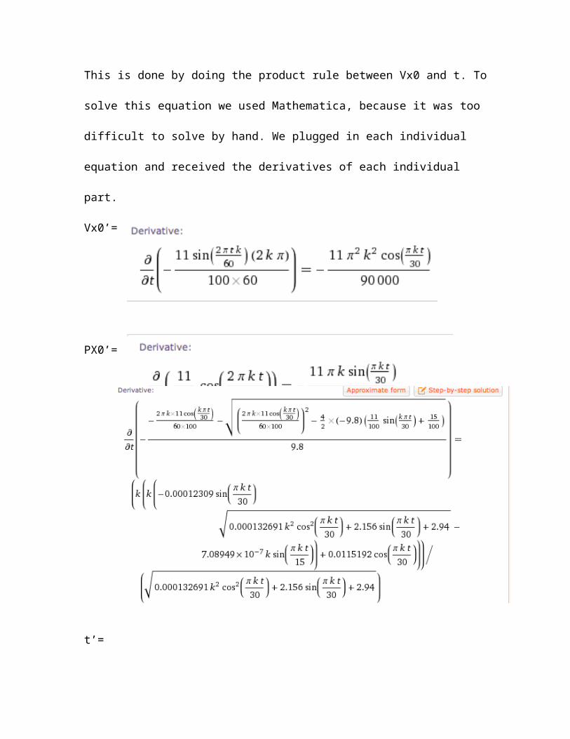
LP’(t0)=(Vx0’)(t)+(Vx0)(t’)+Px0’

This is done by doing the product rule between Vx0 and t. To solve this equation we

used Mathematica, because it was too difficult to solve by hand. We plugged in each

individual equation and received the derivatives of each individual part.

Vx0’=

PX0’=

t’=

3.2 We know from earlier in the lab that the time values of our angles were :

.3257812501 for the angle 5.11735991-(t01)

.3265625003s for the angle 5.12963176-(t02)

We did this earlier in order for solving the launch times of the two different thetas

by solving for t0s by dividing the theta by 2*pi*(K/60) giving us t0. We then plugged

t01 and t02 into the equation |LP(t02)-LP(t01)| in order to estimate LP’(t01)|t02-

t01|. Plugging in our values into the equation| LP(t02)-LP(t01)| we get:

| 0.346892287861652 -0.352155589875231 |=0.005263302

This gives us our estimation of LP’(t01)|t02-t01. We then put in our values of t0 into the latter equation and get

6.80139175055683*(7.812502*10^-4)=0.00531359

Now we can compare the answers 0.005263302 and 0.00531359 and when looking at them we can see that they are extremely close to each other, which means that we are correct.

3.3 We know that .005m<LP’(.35)(delta(t)) (the only reason that we used “<” was

as a guess in order to solve the equation, but either one could work at the

beginning).We also know that LP’(.35)=.47167 to solve this you plug in .35 (the t we

found from 7pi/4) into all of our original functions (PX(t), VX(t),…) when the t is

plugged into all of those functions you can then solve for LP’ because these functions

determine LP. This is done through the use of Mathematica. Therefore we can divide

.005 by LP’(.35) which would give us delta t, and delta t being .0106.

.005m< LP' .35∗(∆t )

.005mLP' .35

=∆ t

.005m

.47167=∆ t

.0106=∆ t

4.1 The acceptable interval of release times is larger at 44.27cm so it would be

harder to be more accurate at 35cm. We decided this from attempting to plot the

graph of LP(theta).

From this drawing of the graph we can see that the wider time interval (drawn in

the white rectangle) is wider than that of the time interval of 44.27cm. This is

because the slope of the line becomes less steep as it goes toward its max value, thus

increasing the range of possible times. So in conclusion from this we can discern

that it is easier to hit the target at 44.27cm because there is a broader time interval.

4.2 We should make the robot spin slower to make the acceptable intervals of

release times larger because when the rotations slow down, it enlarges the possible

times so the robot becomes more accurate. However when we slow down k too

much it will not make the designated target distance, so there is only a certain k that

will give us the largest time range, while still making the distance. To find the most

accurate k and the largest time interval possible to launch the ball to the targeted

distance we used mathematica to plot the graph of LP’(t0). When looking at the

graph we tried to find where the function was equal to zero because this is where

the maxes and mins are on the function, and then found the max throwing distance

at when k was equal to 150. We continued to vary k until we got to the desired

distance of 35cm (targeted distance). Once we found the correct RPM that

minimized the speed (which was 126 RPMs) to get us to 35cm we then found the

time interval for time at which it would still be accurate enough between .5 cm of

the targeted distance, while maintaining k. Doing this gave us our interval of time

which is .412s to .425. We then subtracted the intervals to give us our resolution of

the clock which was .013 seconds, this in comparison to our other resolution is a

100th of a second instead of the 1000th of a second which is much easier for the robot

to do, thus allowing it to launch the ball accurately.

4.3 To explain to a client how to find the appropriate k to use at the distance of 1

meter, you first have to change the target distance that in this case would be 100cm.

Then

Find a list of t where LP’(t)=0, in order to find the max LP(t)

Then plug in one of the t’s in order to find what the max LP(t) is

After realizing the max LP(t) is farther than the targeted distance (100cm), we

reduce the variable K in order to get a t that, when plugged into LP(t), gives us a LP

within 0.5 cm of our 100cm target.

After that, we slightly vary our t value enough that it still gave us an LP within 0.5cm

of our target.

On either side of our t, we get a range of t’s that encompasses our targeted distance

(100cm)

The difference between t’s is our time interval

*sorry if any parts seem a little jumbled, my mind is a little fried so it seemed right

at the time*