0 asymptotic theory for a vector arma-garch model

ASYMPTOTIC THEORY FOR AVECTOR ARMA-GARCH MODEL

SHHHIIIQQQIIINNNGGG LIIINNNGGGHong Kong University of Science and Technology

MIIICCCHHHAAAEEELLL MCCCALLLEEEEEERRRUniversity of Western Australia

This paper investigates the asymptotic theory for a vector autoregressive movingaverage–generalized autoregressive conditional heteroskedasticity~ARMA-GARCH! model+ The conditions for the strict stationarity, the ergodicity, and thehigher order moments of the model are established+ Consistency of the quasi-maximum-likelihood estimator~QMLE! is proved under only the second-ordermoment condition+ This consistency result is new, even for the univariate auto-regressive conditional heteroskedasticity~ARCH! and GARCH models+ More-over, the asymptotic normality of the QMLE for the vector ARCH model isobtained under only the second-order moment of the unconditional errors andthe finite fourth-order moment of the conditional errors+ Under additional mo-ment conditions, the asymptotic normality of the QMLE is also obtained for thevector ARMA-ARCH and ARMA-GARCH models and also a consistent estima-tor of the asymptotic covariance+

1. INTRODUCTION

The primary feature of the autoregressive conditional heteroskedasticity~ARCH!model, as proposed by Engle~1982!, is that the conditional variance of theerrors varies over time+ Such conditional variances have been strongly sup-ported by a huge body of empirical research, especially in stock returns, in-terest rates, and foreign exchange markets+ Following Engle’s pathbreaking idea,many alternatives have been proposed to model conditional variances, form-ing an immense ARCH family; see, for example, the surveys of Bollerslev,Chou, and Kroner~1992!, Bollerslev, Engle, and Nelson~1994!, and Li, Ling,and McAleer~2002!+ Of these models, the most popular is undoubtedly thegeneralized autoregressive conditional heteroskedasticity~GARCH! model ofBollerslev ~1986!+ Some multivariate extensions of these models have beenproposed; see, for example, Engle, Granger, and Kraft ~1984!, Bollerslev, En-gle, and Wooldridge~1988!, Engle and Rodrigues~1989!, Ling and Deng~1993!,

The authors thank the co-Editor, Bruce Hansen, and two referees for very helpful comments and suggestions andacknowledge the financial support of the Australian Research Council+ Address correspondence to: Shiqing Ling,e-mail: maling@ust+hk+

Econometric Theory, 19, 2003, 280–310+ Printed in the United States of America+DOI: 10+10170S0266466603192092

280 © 2003 Cambridge University Press 0266-4666003 $12+00

Engle and Kroner~1995!,Wong and Li~1997!, and Li, Ling, and Wong~2001!,among others+ However, apart from Ling and Deng~1993! and Li, Ling, andWong ~2001!, it seems that no asymptotic theory of the estimators has beenestablished for these multivariate ARCH-type models+ In most of these multi-variate extensions, the primary purpose has been to investigate the structureof the model, as in Engle and Kroner~1995!, and to report empirical findings+

In this paper, we propose a vector autoregressive moving average–GARCH~ARMA-GARCH! model that includes the multivariate GARCH model of Bol-lerslev~1990! as a special case+ The sufficient conditions for the strict station-arity and ergodicity, and a causal representation of the vector ARMA-GARCHmodel, are obtained as extensions of Ling and Li~1997!+ Based on Tweedie~1988!, a simple sufficient condition for the higher order moments of the modelis also obtained+

The main part of this paper investigates the asymptotic theory of the quasi-maximum-likelihood estimator~QMLE! for the vector ARMA-GARCH model+Consistency of the QMLE is proved under only the second-order moment con-dition+ Jeantheau~1998! proves consistency for the constant conditional meandrift model with vector GARCH errors+ His result is based on a modified resultin Pfanzagl~1969!, in which it is assumed that the initial values consisting ofthe infinite past observations are known+ In practice, of course, this is notpossible+

In the univariate case, the QMLE based on any fixed initial values has beeninvestigated by Weiss~1986!, Pantula~1989!, Lee and Hansen~1994!, Lums-daine ~1996!, and Ling and Li~1997!+ Weiss ~1986! and Ling and Li~1997!use the conditions of Basawa, Feign, and Heyde~1976!, whereby their consis-tency results rely on the assumption that the fourth-order moments exist+ Leeand Hansen~1994! and Lumsdaine~1996! use the conditions of Amemiya~1985,pp+ 106–111!, but their methods are only valid for the simple GARCH~1,1!model and cannot be extended to more general cases+ Moreover, the condi-tional errors, that is, h0t whenm 5 1 in equation~2+3! in the next section, arerequired to have the~2 1 k!th ~k . 0! finite moment by Lee and Hansen~1994!and the 32nd finite moment by Lumsdaine~1996!+

The consistency result in this paper is based on a uniform convergence as amodification of a theorem in Amemiya~1985, p+ 116!+ Moreover, the consis-tency of the QMLE for the vector ARMA-GARCH model is obtained only un-der the second-order moment condition+ This result is new, even for the univariateARCH and GARCH models+ For the univariate GARCH~1,1! model, our con-sistency result also avoids the requirement of the higher order moment of theconditional errors, as in Lee and Hansen~1994! and Lumsdaine~1996!+

This paper also investigates the asymptotic normality of the QMLE+ For thevector ARCH model, asymptotic normality requires only the second-ordermoment of the unconditional errors and the finite fourth-order moment of theconditional errors+ The corresponding result for univariate ARCH requires thefourth-order moment, as in Weiss~1986! and Pantula~1989!+ The conditions

ASYMPTOTIC THEORY FOR A VECTOR ARMA-GARCH MODEL 281

for asymptotic normality of the GARCH~1,1! model in Lee and Hansen~1994!and Lumsdaine~1996! are quite weak+ However, their GARCH~1,1! model ex-plicitly excludes the special case of the ARCH~1! model because they assumethat B1 Þ 0 ~see equation~2+7! in Section 2! for purposes of identifiability+Under additional moment conditions, the asymptotic normality of the QMLEfor the general vector ARMA-GARCH model is also obtained+ Given the uni-form convergence result, the proof of asymptotic normality does not need toexplore the third-order derivative of the quasi-likelihood function+ Hence, ourmethod is simpler than those in Weiss~1986!, Lee and Hansen~1994!, Lums-daine~1996!, and Ling and Li~1997!+

It is worth emphasizing that, unlike Lumsdaine~1996! and Ling and Li~1997!,Lee and Hansen~1994! do not assume that the conditional errorsh0t are inde-pendently and identically distributed~i+i+d! instead of a series of strictly station-ary and ergodic martingale differences+Although it is possible to use this weakerassumption for our model, for simplicity we use the i+i+d+ assumption+

The paper is organized as follows+ Section 2 defines the vector ARMA-GARCH model and investigates its properties+ Section 3 presents the quasi-likelihood function and gives a uniform convergence result+ Section 4 establishesthe consistency of the QMLE, and Section 5 develops its asymptotic normality+Concluding remarks are offered in Section 6+ All proofs are given in Appen-dixes A and B+

Throughout this paper, we use the following notation+ The term6{6 denotesthe absolute value of a univariate variable or the determinant of a matrix; 7{7denotes the Euclidean norm of a matrix or vector; A' denotes the transpose ofthe matrix or vectorA; O~1! ~or o~1!! denotes a series of nonstochastic vari-ables that are bounded~or converge to zero!; Op~1! ~or op~1!! denotes a seriesof random variables that are bounded~or converge to zero! in probability; rp

~or rL! denotes convergence in probability~or in distribution!; r~A! denotesthe eigenvalue of the matrixA with largest absolute value+

2. THE MODEL AND ITS PROPERTIES

Bollerslev ~1990! presents anm-dimensional multivariate conditional covari-ance model, namely,

Yt 5 E~Yt 6Ft21! 1 «0t , Var~«0t 6Ft21! 5 D0t G0 D0t , (2.1)

where Ft is the past information available up to timet, D0t 5diag~h01t

102, + + + , h0mt102!, and

G0 5 11 s012 J s01m

s021 1 s023 J

J

s0m,1 J s0m,m21 12 ,

282 SHIQING LING AND MICHAEL MCALEER

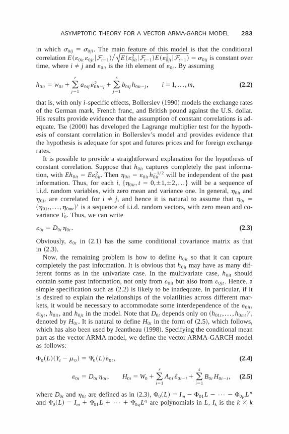
in which s0ij 5 s0ji + The main feature of this model is that the conditionalcorrelationE~«0it «0jt 6Ft21!YYME~«0it

2 6Ft21!E~«0jt2 6Ft21! 5 s0ij is constant over

time, wherei Þ j and«0it is the i th element of«0t + By assuming

h0it 5 w0i 1 (j51

r

a0ij «0it2j2 1 (

j51

s

b0ij h0it2j , i 5 1, + + + ,m, (2.2)

that is, with only i -specific effects, Bollerslev~1990! models the exchange ratesof the German mark, French franc, and British pound against the U+S+ dollar+His results provide evidence that the assumption of constant correlations is ad-equate+ Tse ~2000! has developed the Lagrange multiplier test for the hypoth-esis of constant correlation in Bollerslev’s model and provides evidence thatthe hypothesis is adequate for spot and futures prices and for foreign exchangerates+

It is possible to provide a straightforward explanation for the hypothesis ofconstant correlation+ Suppose thath0it captures completely the past informa-tion, with Eh0it 5 E«0it

2 + Thenh0it 5 «0it h0it2102 will be independent of the past

information+ Thus, for each i, $h0it , t 5 0,61,62, + + + % will be a sequence ofi+i+d+ random variables, with zero mean and variance one+ In general, h0it andh0jt are correlated fori Þ j , and hence it is natural to assume thath0t 5~h01t , + + + ,h0mt!

' is a sequence of i+i+d+ random vectors, with zero mean and co-varianceG0+ Thus, we can write

«0t 5 D0t h0t + (2.3)

Obviously, «0t in ~2+1! has the same conditional covariance matrix as thatin ~2+3!+

Now, the remaining problem is how to defineh0it so that it can capturecompletely the past information+ It is obvious thath0it may have as many dif-ferent forms as in the univariate case+ In the multivariate case, h0it shouldcontain some past information, not only from«0it but also from«0jt + Hence, asimple specification such as~2+2! is likely to be inadequate+ In particular, if itis desired to explain the relationships of the volatilities across different mar-kets, it would be necessary to accommodate some interdependence of the«0it ,«0jt , h0it , andh0jt in the model+ Note thatD0t depends only on~h01t , + + + , h0mt!

' ,denoted byH0t + It is natural to defineH0t in the form of ~2+5!, which follows,which has also been used by Jeantheau~1998!+ Specifying the conditional meanpart as the vector ARMA model, we define the vector ARMA-GARCH modelas follows:

F0~L!~Yt 2 m0! 5 C0~L!«0t , (2.4)

«0t 5 D0t h0t , H0t 5 W0 1 (i51

r

A0i ?«0t2i 1 (i51

s

B0i H0t2i , (2.5)

whereD0t andh0t are defined as in~2+3!, F0~L! 5 Im 2 F01L 2 {{{ 2 F0pLp

and C0~L! 5 Im 1 C01L 1 {{{ 1 C0qLq are polynomials inL, Ik is the k 3 k


identity matrix, and ?«0t 5 ~«01t2 , + + + ,«0mt

2 !' + The true parameter vector is de-noted by l0 5 ~w0

' ,d0' ,s0

'!' , where w0 5 vec~m0,F01, + + + ,F0p,C01, + + + ,C0q!,d0 5 vec~W0,A01, + + + ,A0r , B01, + + + ,B0s!, and s0 5 ~s021, + + + ,s0m,1,s032, + + + ,s0m,2, + + + ,s0m,m21!' + This model was used to analyze the Hang Seng index andStandard and Poor’s 500 Composite index by Wong, Li , and Ling~2000!+ Theyfound that the off-diagonal elements inA01 are significantly different fromzero and hence can be used to explain the volatility relationship between thetwo markets+

The model for the unknown parameterl 5 ~w ',d ',s '!' , with w, d, and sdefined in a similar manner tow0, d0, ands0, respectively, is

F~L!~Yt 2 m! 5 C~L!«t , (2.6)

Ht 5 W1 (i51

r

Ai ?«t2i 1 (i51

s

Bi Ht2i , (2.7)

whereHt 5 ~h1t , + + + , hmt!' , ?«t 5 ~«1t

2 , + + + ,«mt2 !' , andF~L! andC~L! are defined

in a similar manner toF0~L! and C0~L!, respectively+ First, the «t are com-puted from the observationsY1, + + + ,Yn, from ~2+6!, with initial value PY0 5~Y0, + + + ,Y12p,«0, + + + ,«12q!+ Then Ht can be calculated from~2+7!, with initialvalues S«0 5 ~ ?«0, + + + , ?«12r ,H0, + + + ,H12s!+We assume that the parameter spaceQis a compact subspace of Euclidean space, such thatl0 is an interior point inQand, for eachl [ Q, we make the following assumptions+

Assumption 1+ All the roots of 6F~L!6 5 0 and all the roots of6C~L!6 5 0are outside the unit circle+

Assumption 2+ The termsF~L! andC~L! are left coprime~i+e+, if F~L! 5U~L!F1~L! and C~L! 5 U~L!C1~L!, then U~L! is unimodular with constantdeterminant! and satisfy other identifiability conditions given in Dunsmuir andHannan~1976!+

Assumption 3+ The matrixG is a finite and positive definite symmetric ma-trix, with the elements on the diagonal being 1 andr~G! having a positivelower bound overQ; all the elements ofAi andBj are nonnegative, i 5 1, + + + , r,j 5 1, + + + ,s; each element ofW has positive lower and upper bounds overQ;and all the roots of6 Im 2 (i51

r Ai Li 2 (i51

s Bi Li 6 5 0 are outside the unit

circle+

Assumption 4+ Im 2 (r51r Ai L

i and (i51s Bi L

i are left coprime and satisfyother identifiability conditions given in Jeantheau~1998! ~see also Dunsmuirand Hannan, 1976!+

In Assumptions 2 and 4, we use the identifiability conditions in Dunsmuirand Hannan~1976! and Jeantheau~1998!+ These conditions may be too strong+Alternatively, we can use other identifiability conditions, such as the final formor echelon form in Lütkepohl~1993, Ch+ 7!, under which the results in thispaper for consistency and asymptotic normality will still hold with some minor


modifications+ These identifiability conditions are sufficient for the proofs of~B+3! and~B+6! in Appendix B+

Note that, under Assumption 4, Bs Þ 0 and hence the ARCH and GARCHmodels are nonnested+ We define the ARMA-ARCH model as follows:

F0~L!~Yt 2 m0! 5 C0~L!«0t , (2.8)

«0t 5 D0t h0t , H0t 5 W0 1 (i51

r

A0i ?«0t2i + (2.9)

Similarly, under Assumption 2, it is not allowed that all the coefficients in theARMA model are zero, so that the ARMA-ARCH model does not include thefollowing ARCH model as a special case:

Yt 5 m0 1 «0t , (2.10)

«0t 5 D0t h0t , H0t 5 W0 1 (i51

r

A0i ?«0t2i + (2.11)

In models~2+8! and~2+9! and~2+10! and~2+11!, we assume that all the compo-nents ofA0i , i 5 1, + + + , r, are positive+ In practice, this assumption may be toostrong+ If the parameter matricesAi are assumed to have the nested reduced-rank form, as in Ahn and Reinsel~1988!, then the results in this and the follow-ing sections will still hold with some minor modifications+

The unknown parameter ARCH and ARMA-ARCH models are defined sim-ilarly to models~2+6! and ~2+7!+ The true parameterl0 5 ~w0

' ,d0' ,s0

'!' , withd0 5 vec~W0,A01, + + + ,A0r !, s0 being defined as in models~2+4! and ~2+5!, andw0 being defined as in models~2+4! and ~2+5! for models ~2+8! and ~2+9!,and w0 5 m0 for models ~2+10! and ~2+11!+ Similarly, define the unknownparameterl and the parametric spaceQ, with 0 , aijk

l # aijk # aijku , `,

whereaijk is the ~ j, k!th component ofAi , aijkl and aijk

u are independent ofl,i 5 1, + + + , r, and j, k 5 1, + + + ,m+1

The following theorem gives some basic properties of models~2+4! and~2+5!+Whenm 5 1, the result in Theorem 2+1 reduces to that in Ling and Li~1997!and the result in Theorem 2+2 reduces to Theorem 6+2 in Ling ~1999! ~see alsoLing and McAleer, 2002a, 2002b!+ When the ARMA model is replaced by aconstant mean drift, the second-order stationarity and ergodicity condition inTheorem 2+1 appears to be the same as Proposition 3+1 in Jeantheau~1998!+Our proof is different from that in his paper and provides a useful causal ex-pansion+ Also note that, in the following theorems, Assumptions 2 and 4 arenot imposed and hence these results hold for models~2+8! and ~2+9! and mod-els~2+10! and~2+11!+ However, for these two special cases, the matrix DA0t , whichfollows, can simply be replaced by its~1,1! block+

THEOREM 2+1+ Under Assumptions 1 and 3, models (2.4) and (2.5) possessanFt-measurable second-order stationary solution$Yt ,«0t ,H0t %, which is unique,given theh0t, whereFt is a s-field generated by$h0k : k # t %. The solutions$Yt % and $H0t % have the following causal representations:


Yt 5 (k50

`

Y0k«0t2k, a+s+ , (2.12)

H0t 5 W0 1 (j51

`

c'S)i51

j

DA0t2iDjt2j21, a+s+ , (2.13)

whereF021~L!C0~L! 5 (k50

` Y0kLk, jt 5 @~ Ih0t W0!',0, + + + ,0,W0' ,0, + + + ,0# ~r1s!m31

' ,that is, the subvector consisting of the first m components isIh0tW0 and thesubvector consisting of the~rm 1 1!th to ~r 1 1!mth components is W0; Ih0t 5diag~h01t

2 , + + + ,h0mt2 !, c' 5 ~0, + + + ,0, Im,0, + + + ,0!m3~r1s!m with the subvector con-

sisting of the~rm 1 1!th to ~r 1 1!mth columns being Im; and

DA0t 5 1Ih0t A01 J Ih0t A0r Ih0t B01 J Ih0t B0s

Im~r21! Om~r21!3m Om~r21!3ms

A01 J A0r B01 J B0s

Om~s21!3mr Im~s21! Om~s21!3m

2 +Hence,$Yt ,«0t ,H0t % are strictly stationary and ergodic.

THEOREM 2+2+ Suppose that the assumptions of Theorem 2.1 hold. Ifr@E~ DA0t

Jk!# , 1, with k being a strictly positive integer, then the2kth mo-ments of$Yt ,«0t % are finite, where DA0t is defined as in Theorem 2.1 and AJk isthe Krönecker product of the k matrices A.

3. QUASI-MAXIMUM-LIKELIHOOD ESTIMATOR

The estimators of the parameters in models~2+4! and~2+5! are obtained by max-imizing, conditional on~ PY0, S«0!,

Ln~l! 51

n (t51

n

l t ~l!, l t ~l! 5 21

2ln6Dt GDt 62

1

2«t'~Dt GDt !

21«t , (3.1)

whereLn~l! takes the form of the Gaussian log-likelihood andDt 5 diag~h1t102,

+ + + , hmt102!+ Because we do not assume thath0t is normal, the estimators from

~3+1! are the QMLEs+ Note that the processes«i andDi , i # 0, are unobservedand hence they are only some chosen constant vectors+ Thus, Ln~l! is the like-lihood function that is not conditional on the true~ PY0, S«0! and, in practice, wework with this likelihood function+

For convenience, we introduce the unobserved process$~«te ,Ht

e! : t 5 0,61,62, + + + % , which satisfies

F~L!~Yt 2 m! 5 C~L!«te , (3.2)

Hte 5 W1 (

i51

r

Ai ?«t2ie 1 (

i51

s

Bi Ht2ie , (3.3)


where ?«te 5 ~«1t

e2, + + + ,«mte2!' andHt

e 5 ~h1te , + + + , hmt

e !' + Denote sY0 5 ~Y0,Y21, + + + !+The unobserved log-likelihood function conditional onsY0 is

Lne ~l! 5

1

n (t51

n

l te~l!, l t

e~l! 5 21

2ln6Dt

e GDte 62

1

2«t

e '~Dte GDt

e!21«te , (3.4)

whereDte 5 diag~h1t

e , + + + , hmte !+ Whenl 5 l0, we have«t

e 5 «0t , Hte 5 H0t , and

Dte 5 D0t + The primary difference in the likelihoods~3+1! and~3+4! is that~3+1!

is conditional on any initial values, whereas~3+4! is conditional on the infinitepast observations+ In practice, the use of~3+4! is not possible+ Jeantheau~1998!investigates the likelihood~3+4! for models~2+4! and~2+5! with p 5 q 5 0, thatis, with the conditional mean part identified as the constant drift+ By modifyinga result in Pfanzagl~1969!, he proves the consistency of the QMLE for a spe-cial case of models~2+4! and~2+5!+ An improvement on his result requires onlythe second-order moment condition+ However, the method of his proof is validonly for the log-likelihood function~3+4!, and it is not clear whether his resultalso holds for the likelihood~3+1!+

The likelihood functionLn~l! and the unobserved log-likelihood functionLn

« ~l! for models~2+8! and ~2+9! and models~2+10! and ~2+11! are similarlydefined as in~3+1! and~3+4!+

The following uniform convergence theorem is a modification of Theo-rem 4+2+1 in Amemiya~1985!+ This theorem, and also Lemma 4+5 in the nextsection, makes it possible to prove the consistency of the QMLE from the like-lihood ~3+1! under only a second-order moment condition+

THEOREM 3+1+2 Let g~ y,u! be a measurable function of y in Euclideanspace for eachu [ Q, a compact subset of Rm (Euclidean m-space), anda continuous function ofu [ Q for each y. Suppose that yt is a sequenceof strictly stationary and ergodic time series, such that Eg~ yt ,u! 5 0 andE supu[Q6g~ yt ,u!6 , `. Thensupu[Q 6n21 (t51

n g~ yt ,u!6 5 op~1!.

4. CONSISTENCY OF THE QMLE

In ~3+4!, Dte is evaluated by an infinite expansion of~3+3!+We need to show that

such an expansion is convergent+ In general, all the roots of6 Im 2 (i51r Ai L

i 2

(i51s Bi L

i 65 0 lying outside the unit circle does not ensure that all the roots of6 Im 2 (i51

s Bi Li 6 5 0 are outside the unit circle+ However, because all the ele-

ments ofAi andBi are negative, we have the following lemma+

LEMMA 4 +1+ Under Assumption 3, all the roots of6 Im 2 (i51s Bi L

i 65 0 areoutside the unit circle.

We first present five lemmas+ Lemma 4+2 ensures the identification ofl0+Lemmas 4+3, 4+4, and 4+6 ensure that the likelihoodLn~l! of the ARMA-GARCH, ARMA-ARCH, and ARCH models converges uniformly in the wholeparameter space, with its limit attaining a unique maximum atl0+ Lemma 4+5


is important for the proof of Lemma 4+6 under the second-order momentcondition+

LEMMA 4 +2+ Suppose that Yt is generated by models (2.4) and (2.5)satisfying Assumptions 1–4, or models (2.8) and (2.9) satisfying Assumptions1–3, or models (2.10) and (2.11) satisfying Assumption 3. Let cw and c beconstant vectors, with the same dimensions asw and d, respectively. Thencw' ~]«t

e ' 0]w! 5 0 a.s. only if cw 5 0, and c'~]Hte ' 0]d! 5 0 a.s. only if c5 0.

LEMMA 4 +3+ Define L~l! 5 E @l te~l!# . Under the assumptions of Lemma

4+2, L~l! exists for alll [ Q and supl[Q 6Lne ~l! 2 L~l!6 5 op~1!.

LEMMA 4 +4+ Under the assumptions of Lemma 4.2, L~l! achieves a uniquemaximum atl0.

LEMMA 4 +5+ Let Xt be a strictly stationary and ergodic time series, withE6Xt 6 , `, andjt be a sequence of random variables such that

sup1#t#n

6jt 6 # C and n21 (t51

n

6jt 65 op~1!+

Then n21 (t51n Xt jt 5 op~1!.

LEMMA 4 +6+ Under the assumptions of Lemma 4.2,supl[Q 6Lne ~l! 2

Ln~l!6 5 op~1!.

Based on the preceding lemmas, we now have the following consistencytheorem+

THEOREM 4+1+ Denote Zln as the solution tomaxl[Q Ln~l!. Under the as-sumptions of Lemma 4.2,Zln rp l0.

5. ASYMPTOTIC NORMALITY OF THE QMLE

To prove the asymptotic normality of the QMLE, it is inevitable to explore thesecond derivative of the likelihood+ The method adopted by Weiss~1986!, Leeand Hansen~1994!, Lumsdaine~1996!, and Ling and Li~1997! uses the thirdderivative of the likelihood+ By using Theorem 3+1, our method requires onlythe second derivative of the likelihood, which simplifies the proof and reducesthe requirement for higher order moments+

For the general models~2+4! and~2+5!, the asymptotic normality of the QMLEwould require the existence of the sixth moment+ However, for models~2+8!and ~2+9! or models~2+10! and ~2+11!, the moment requirements are weaker+Now we can state some basic results+

LEMMA 5 +1+ Suppose that Yt is generated by models (2.4) and (2.5) satis-fying Assumptions 1–4, or models (2.8) and (2.9) satisfying Assumptions 1–3,or models (2.10) and (2.11) satisfying Assumption 3. Then, it follows that


E supl[Q

** ]«te '

]w~Dt

e GDte!21

]«te

]w ' ** , ` and EF ]«te '

]w~Dt

e GDte!21

]«te

]w 'G . 0,

(5.1)

where a matrix A. 0 means that A is positive definite.

LEMMA 5 +2+ Suppose that Yt is generated by models (2.4) and (2.5) satis-fying Assumptions 1–4 and E7Yt74 , `, or models (2.8) and (2.9) satisfyingAssumptions 1–3 and E7Yt74 , `, or models (2.10) and (2.11) satisfying As-sumption 3 and E7h0t74 , `. ThenV0 5 E @~]l0t

e 0]l!~]l0te 0]l' !# is finite+ Fur-

thermore, if V0 . 0, then

1

Mn (t51

n ]l0t

]lrL N~0,V0!,

where]l0t« 0]l 5 ]l t

«0]l 6l0and ]l0t 0]l 5 ]l t 0]l 6l0

.

LEMMA 5 +3+ Suppose that Yt is generated by models (2.4) and (2.5) satis-fying Assumptions 1–4 and E7Yt76 , `, or models (2.8) and (2.9) satisfyingAssumptions 1–3 and E7Yt74 , `, or models (2.10) and (2.11) satisfying As-sumption 3. Then,

E supl[Q

** ]Hte '

] DlDt

e22Dte Dt

e22]Ht

e

] Dl' ** , `, (5.2)

where Dl 5 ~w ',d '!', Dte 5 Iht

e G21 Ihte 1 DDt

e Ihte , DDt

e 5 diag~e1G21hte , + + + ,emG21ht

e!,ei 5 ~0, + + + , 0,1,0, + + + ,0!' of which the ith element is 1,ht

e 5 ~h1te , + + + ,hmt

e !', andIhte 5 diag~h1t

e , + + + ,hmte ! with hit

e 5 «ite0hit

e102, i 5 1, + + + ,m.

LEMMA 5 +4+ Under the assumptions of Lemma 5.3,

(a) supl[Q

** 1

n (t51

n ]2l te

]l]l'2 EF ]2l t

e

]l]l' G**5 op~1!,

(b) supl[Q

** 1

n (t51

n F ]2l te

]l]l'2

]2l t]l]l' G**5 op~1!+

By straightforward calculation, we can show that

S0 [ EF ]2l te

]l]l'G

l0

5 2S S Dl0 S Dls0

S Dls0'

1

2P'PD,

where S Dl0 5 E @~]«0te ' 0] Dl!~D0t G0 D0t !

21~]«0te 0] Dl' !# 1 E @~]H0t

e ' 0] Dl!D0t22 3

CD0t22~]H0t

e 0] Dl'!#04, S Dls0 5 E @~]H0te ' 0] Dl!D0t

22#C1 P02, ]«0te 0] Dl' 5 ]«t

e0] Dl' 6l0,

]H0te 0] Dl' 5 ]Ht

e0] Dl' 6l0, P 5 ~Im J G0

21!K, C1 5 ~C11, + + + ,C1m!, C1i is anm 3 m matrix with the~i, i !th component being 1 and the other componentszero, K 5 ] vec~G!0]s ' is a constant matrix, andC 5 G0

21 ( G0 1 Im, where


A ( B 5 ~aij bij ! for two matricesA 5 ~aij ! and B 5 ~bij !+ In practice, S0 isevaluated by

ZSn 5 2S ZS Dl ZS Dls

ZS Dls'

1

2ZP' ZPD,

where ZGn 5 G6 Zln,

ZS Dl 51

n (t51

n F ]«t'

] Dl~Dt GDt !

21]«t

] Dl' G Zln

11

4n (t51

n F ]Ht'

] DlDt

22 ZCn Dt22

]Ht

] Dl' G Zln

,

ZS Dls 51

2n (t51

n F ]Ht'

] DlDt

22GZln

C1 ZP, ZP 5 ~Im J ZGn21!K,

ZCn 5 ZGn21 ( ZGn 1 Im+

LEMMA 5 +5+ Under the assumptions of Lemma 5.3,7S07 , ` and ZSn 5S0 1 op~1! for any sequenceln, such thatln 2 l0 5 op~1!. If G0

21 ( G0 $ Im,then2S0 . 0.

From the proof, we can see that the sixth-order moment in models~2+4! and~2+5! is required only for Lemma 5+4~a!, whereas the fourth-order moment issufficient for Lemma 5+4~b!+ If we can show that the convergent rate of theQMLE is Op~n2102!, then the fourth-order moment is sufficient for models~2+4!and~2+5!+ However, it would seem that proving the rate of convergence is quitedifficult +

LEMMA 5 +6+ Under the assumptions of Lemma 5.2, ifMn~ln 2 l0! 5Op~1!, then

(a)1

n (t51

n F ]l te

]l

]l te

]l'2

]l0te

]l

]l0te

]l'G

ln

5 op~1!,

(b) ZVn [1

n (t51

n F ]l t]l

]l t]l'

Gln

5 V0 1 op~1!+

THEOREM 5+1+ Suppose that Yt is generated by models (2.4) and (2.5)satisfying Assumptions 1–4 and E7Yt76 , `, or models (2.8) and (2.9) satis-fying Assumptions 1–3 and E7Yt74 , `, or models (2.10) and (2.11) satisfy-ing Assumption 3 and E7h0t74 , `. If V0 . 0 and G0

21 ( G0 $ Im, thenMn~ Zln 2 l0! rL N~0,S0

21V0S021!. Furthermore, S0 and V0 can be estimated

consistently by ZSn and ZVn, respectively.

Whenm5 1 or 2, we can show thatG021 ( G0 $ Im, and hence, in this case,

2S0 . 0+ However, it is difficult to prove G021 ( G0 $ Im for the general case+

WhenG0 5 Im, it is straightforward to show that2S0 . 0 andV0 are positivedefinite+ Whenh0t follows a symmetric distribution,


V0 5 E1]l0t

e

]w

]l0te

]w '0

0]l0t

e

] Dd]l0t

e

] Dd '2 and S0 5 2SSw0 0

0 S Dd0D,

in which Dd 5 ~d ',s '!' ,

Sw0 5 EF ]«0te '

]w~D0t G0 D0t !

21]«0t

e

]w 'G1

1

4EF ]H0t

e '

]wD0t

22CD0t22

]H0te

]w 'G ,

S Dd0 5 S Sd0 Sds0

Sds0'

1

2P'PD,

where Sd0 5 E @]H0te ' 0]dD0t

22CD0t22]H0t

e 0]d ' #04 and Sds0 5 E @]H0te ' 0

]dD0t22#C1 P02+ Furthermore, if h0t is normal, it follows that 2S0 5 V0+ Note

that the QMLE here is the global maximum over the whole parameter space+The requirement of the sixth-order moment is quite strong for models~2+4! and~2+5! and is used only because we need to verify the uniform convergence ofthe second derivative of the log-likelihood function, that is, Lemma 5+4~a!+ Ifwe consider only the local QMLE, then the fourth-order moment is sufficient+For univariate cases, such proofs can be found in Ling and Li~1998! and Lingand McAleer~2003!+

6. CONCLUSION

This paper presented the asymptotic theory for a vector ARMA-GARCH model+An explanation of the proposed model was offered+ Using a similar idea, dif-ferent multivariate models such as E-GARCH, threshold GARCH, and asym-metric GARCH can be proposed for modeling multivariate conditionalheteroskedasticity+ The conditions for the strict stationarity and ergodicity ofthe vector ARMA-GARCH model were obtained+ A simple sufficient condi-tion for the higher order moments of the model was also provided+ We estab-lished a uniform convergence result by modifying a theorem in Amemiya~1985!+ Based on the uniform convergence result, the consistency of the QMLEwas obtained under only the second-order moment condition+ Unlike Weiss~1986! and Pantula~1989! for the univariate case, the asymptotic normality ofthe QMLE for the vector ARCH model requires only the second-order mo-ment of the unconditional errors and the finite fourth-order moment of theconditional errors+ The asymptotic normality of the QMLE for the vectorARMA-ARCH model was proved using the fourth-order moment, which is anextension of Weiss~1986! and Pantula~1989!+ For the general vector ARMA-GARCH model, the asymptotic normality of the QMLE requires the assump-tion that the sixth-order moment exists+ Whether this result will hold undersome weaker moment conditions remains to be proved+


NOTES

1+ For models~2+8! and ~2+9! and ~2+10! and ~2+11!, Bi in Assumption 3 reduces to the zeromatrix, wherei 5 1, + + + ,s+

2+ The co-editor has suggested that this theorem may not be new, consisting of Lemma 2+4 andfootnote 18 of Newey and McFadden~1994!+

REFERENCES

Ahn, S+K+ & Reinsel, G+C+ ~1988! Nested reduced-rank autoregressive models for multiple timeseries+ Journal of the American Statistical Association83, 849–856+

Amemiya, T+ ~1985! Advanced Econometrics+ Cambridge: Harvard University Press+Basawa, I+V+, P+D+ Feign, & C+C+ Heyde~1976! Asymptotic properties of maximum likelihood es-

timators for stochastic processes+ Sankhya A38, 259–270+Bollerslev, T+ ~1986! Generalized autoregressive conditional heteroskedasticity+ Journal of Econo-

metrics31, 307–327+Bollerslev, T+ ~1990! Modelling the coherence in short-run nominal exchange rates: A multivariate

generalized ARCH approach+ Review of Economics and Statistics72, 498–505+Bollerslev, T+, R+Y+ Chou, & K +F+ Kroner ~1992! ARCH modelling in finance: A review of the

theory and empirical evidence+ Journal of Econometrics52, 5–59+Bollerslev, T+, R+F+ Engle, & D +B+ Nelson~1994! ARCH models+ In R+F+ Engle and D+L+ McFadden

~eds+!, Handbook of Econometrics, vol+ 4, pp+ 2961–3038+ Amsterdam: North-Holland+Bollerslev, T+, R+F+ Engle, & J+M+Wooldridge~1988! A capital asset pricing model with time vary-

ing covariance+ Journal of Political Economy96, 116–131+Chung, K+L+ ~1968! A Course in Probability Theory+ New York: Harcourt Brace+Dunsmuir, W+ & E+J+ Hannan~1976! Vector linear time series models+ Advances in Applied Prob-

ability 8, 339–364+Engle, R+F+ ~1982! Autoregressive conditional heteroskedasticity with estimates of variance of U+K+

inflation+ Econometrica50, 987–1008+Engle, R+F+, C+W+J+ Granger, & D +F+ Kraft ~1984! Combining competing forecasts of inflation using

a bivariate ARCH model+ Journal of Economic Dynamics and Control8, 151–165+Engle, R+F+ & K +F+ Kroner~1995!+Multivariate simultaneous generalized ARCH+ Econometric Theory

11, 122–150+Engle, R+F+ & A +P+ Rodrigues~1989! Tests of international CAPM with time varying covariances+

Journal of Applied Econometrics4, 119–128+Harville, D+A+ ~1997! Matrix Algebra from a Statistician’s Perspective+ New York: Springer-Verlag+Jeantheau, T+ ~1998! Strong consistency of estimators for multivariate ARCH models+ Econometric

Theory14, 70–86+Johansen, S+ ~1995! Likelihood-Based Inference in Cointegrated Vector Autoregressive Models+ New

York: Oxford University Press+Lee, S+-W+ & B +E+ Hansen~1994! Asymptotic theory for the GARCH~1,1! quasi-maximum likeli-

hood estimator+ Econometric Theory10, 29–52+Li , W+K+, S+ Ling, & M + McAleer ~2002! Recent theoretical results for time series models with

GARCH errors+ Journal of Economic Surveys16, 245–269+ Reprinted in M+ McAleer and L+Oxley ~eds+!, Contributions to Financial Econometrics: Theoretical and Practical Issues~Ox-ford: Blackwell, 2002!, pp+ 9–33+

Li ,W+K+, S+ Ling, & H +Wong~2001! Estimation for partially nonstationary multivariate autoregres-sive models with conditional heteroskedasticity+ Biometrika88, 1135–1152+

Ling, S+ ~1999! On the probabilistic properties of a double threshold ARMA conditional heteroske-dasticity model+ Journal of Applied Probability3, 1–18+

Ling, S+ & W+C+ Deng~1993! Parametric estimate of multivariate autoregressive models with con-ditional heterocovariance matrix errors+ Acta Mathematicae Applicatae Sinica16, 517–533~inChinese!+


Ling, S+ & W+K+ Li ~1997! On fractionally integrated autoregressive moving-average time seriesmodels with conditional heteroskedasticity+ Journal of the American Statistical Association92,1184–1194+

Ling, S+ & W+K+ Li ~1998! Limiting distributions of maximum likelihood estimators for unstableARMA models with GARCH errors+ Annals of Statistics26, 84–125+

Ling, S+ & M + McAleer ~2002a! Necessary and sufficient moment conditions for the GARCH~r,s!and asymmetric power GARCH~r,s! models+ Econometric Theory18, 722–729+

Ling, S+ & M + McAleer ~2002b! Stationarity and the existence of moments of a family of GARCHprocesses+ Journal of Econometrics106, 109–117+

Ling, S+ & M +McAleer ~2003! On adaptive estimation in nonstationary ARMA models with GARCHerrors+ Annals of Statistics, forthcoming+

Lumsdaine, R+L+ ~1996! Consistency and asymptotic normality of the quasi-maximum likelihoodestimator in IGARCH~1,1! and covariance stationary GARCH~1,1! models+ Econometrica64,575–596+

Lütkepohl, H+ ~1993! Introduction to Multiple Time Series Analysis, 2nd ed+ Berlin: Springer-Verlag+Newey, W+K+ & D +L+ McFadden~1994! Large sample estimation and hypothesis testing+ In R+F+

Engle and D+L+ McFadden~eds+!, Handbook of Econometrics, vol+ 4, pp+ 2111–2245, Amster-dam: Elsevier+

Pantula, S+G+ ~1989! Estimation of autoregressive models with ARCH errors+ Sankhya B50, 119–138+Pfanzagl, J+ ~1969! On the measurability and consistency of minimum contrast estimates+ Metrika

14, 249–272+Stout, W+F+ ~1974! Almost Sure Convergence+ New York: Academic Press+Tse, Y+K+ ~2000! A test for constant correlations in a multivariate GARCH model+ Journal of Econo-

metrics98, 107–127+Tweedie, R+L+ ~1988! Invariant measure for Markov chains with no irreducibility assumptions+ Jour-

nal of Applied Probability25A, 275–285+Weiss, A+A+ ~1986! Asymptotic theory for ARCH models: Estimation and testing+ Econometric

Theory2, 107–131+Wong, H+ & W+K+ Li ~1997! On a multivariate conditional heteroscedasticity model+ Biometrika4,

111–123+Wong, H+, W+K+ Li , & S+ Ling ~2000! A Cointegrated Conditional Heteroscedastic Model with

Financial Applications, Technical report, Department of Applied Mathematics, Hong Kong Poly-technic University+

APPENDIX A: PROOFS OFTHEOREMS 2+1 AND 2+2

Proof of Theorem 2.1. Multiplying ~2+5! by Ih0t yields

?«0t 5 Ih0t W0 1 (i51

r

Ih0t A0i ?«0t2i 1 (i51

s

Ih0t B0i H0t2i + (A.1)

Now rewrite~A+1! in vector form as

Xt 5 DA0t Xt21 1 jt , (A.2)

whereXt 5 ~ ?«0t' , + + + , ?«0t2r11

' ,H0t' , + + + ,H0t2s11

' !' andjt is defined as in~2+13!+ Let

Sn, t 5 jt 1 (j51

n S)i51

j

DA0t2i11D jt2j , (A.3)


wheren 5 1,2, + + + + Denote thekth element of~) i51j DA0t2i !jt2j21 by sn, t + We have

E6sn, t 6 5 ek'ES)

i51

j

DA0t2iDjt2j21

5 ek'S)

i51

j

E DA0t2iDEjt2j21 5 ek' DAjc*, (A.4)

whereek 5 ~0, + + + ,0,1,0, + + + ,0!m~r1s!31' and 1 appears in thekth position, c* 5 Ejt is a

constant vector, and

DA 5 1A01 J A0r B01 J B0s

Im~r21! Om~r21!3m Om~r21!3ms

A01 J A0r B01 J B0s

Om~s21!3mr Im~s21! Om~s21!3m

2 + (A.5)

By direct calculation, we know that the characteristic polynomial ofDA is

f ~z! 5 6z6~r1s!m6 Im 2 (i51

r

Ai z2i 2 (i51

s

Bi z2i 6+ (A.6)

By Assumption 3, it is obvious that all the roots off ~z! lie inside the unit circle+ Thus,r~ DA! , 1, and hence each component ofDAi is O~ r i !+ Therefore, the right-hand side of~A+4! is equal toO~ r j !+ Note that Ih0t is a sequence of i+i+d+ random matrices and eachelement of DA0t andjt is nonnegative+ We know that each component ofSn, t convergesalmost surely~a+s+! asn r `, as doesSn, t + Denote the limit ofSn, t by Xt + We have

Xt 5 jt 1 (j51

` S)i51

j

DA0t2iDjt2j21, (A.7)

with the first-order moment being finite+It is easy to verify thatXt satisfies~A+2!+ Hence, there exists anFt -measurable second-

order solution«0t to ~2+5! with i th element«0it 5 h0itMh0it 5 h0it ~erm1i' Xt !

102, with therepresentation~2+13!+

Now we show that such a solution is unique to~2+5!+ Let «t~1! be anotherFt -measur-

able second-order stationary solution of~2+5!+ As in ~A+2!, we haveXt~1! 5 DA0t Xt21

~1! 1

jt , whereXt~1! 5 ~ ?«t

~1!' , + + + , ?«t2r11~1!' ,Ht

~1!' , + + + ,Ht2s11~1!' !' andHt

~1! 5 W0 1 (i51r A0i ?«t2i

~1! 1

(i51s B0i Ht2i

~1! with ?«t~1! 5 ~«1t

~1!2, + + + ,«mt~1!2!' + Let Ut 5 Xt 2 Xt

~1!+ Then Ut is first-orderstationary and, by ~A+2!, Ut 5 ~) i50

n DA0t2i !Ut2n21+ Denote thekth component ofUt

asuk, t + Then, as each element ofDAt is nonnegative,

6ukt 6 # 6ek'S)

i50

n

DA0t2iDUt2n216# ek'S)

i50

n

DA0t2iD6Ut2n216, (A.8)

whereek is defined as in~A+4! and 6Ut 6 is defined as~6u1t 6, + + + ,6u~r1s!m, t 6!' + As Ut isfirst-order stationary andFt -measurable, by ~A+8!, we have

E6ukt 6 # ek'ES)

i50

n

DA0t2iDE6Ut2n2165 ek' DAnc1

*r 0 (A.9)


asn r `, wherec1* 5 E6Ut 6 is a constant vector+ So ukt 5 0 a+s+, that is, Xt 5 Xt

~1! a+s+Thus, hit 5 hit

~1! a+s+, and hence«0t 5 «0t~1! 5 h0it h0it

102 a+s+ That is, «0t satisfying~2+5! isunique+

For the unique solution«0t , by the usual method, we can show that there exists auniqueFt -measurable second-order stationary solutionYt satisfying~2+4!, with the ex-pansion given by

Yt 5 (k50

`

Y0k«0t2k+ (A.10)

Note that the solution$Yt ,«0t ,H0t % is a fixed function of a sequence of i+i+d+ randomvectorsh0t and hence is strictly stationary and ergodic+ This completes the proof+ n

The proof of Theorem 2+2 first transforms models~2+4! and~2+5! into a Markov chainand then uses Tweedie’s criterion+ Let $Xt ; t 5 1,2, + + + % be a temporally homogeneousMarkov chain with a locally compact completely separable metric state space~S,B!+The transition probability isP~x,A! 5 Pr~Xn [ A6Xn21 5 x!, wherex [ S andA [ B+Tweedie’s criterion is the following lemma+

LEMMA A +1+ ~Tweedie, 1988, Theorem 2!+ Suppose that$Xt % is a Feller chain.

(1) If there exist, for some compact set A[ B, a nonnegative function g and« . 0satisfying

EAc

P~x,dy!g~ y! # g~x! 2 «, x [ Ac, (A.11)

then there exists as-finite invariant measurem for P with 0 , m~A! , `.(2) Furthermore, if

EA

m~dx!FEAc

P~x,dy!g~ y!G , `, (A.12)

thenm is finite, and hencep 5 m0m~S! is an invariant probability.(3) Furthermore, if

EAc

P~x,dy!g~ y! # g~x! 2 f ~x!, x [ Ac, (A.13)

thenm admits a finite f-moment, that is,

ES

m~dy! f ~ y! , `+ (A.14)

The following two lemmas are preliminary results for the proof of Theorem 2+2+

LEMMA A +2+ Suppose that E~7h0t72k! , ` andr@E~ DA0tJk!# , 1. Then there exists a

vector M . 0 such that@Im 2 E~ DA0tJk!' #M . 0, where a vector B. 0 means that each

element of B is positive.


Proof. From the condition given, Im 2 E~ DA0tJk! is invertible+ Because each element

of E~ DA0tJk! is nonnegative, we can choose a vectorL1 . 0 such that

M :5 @Im 2 E~ DA0tJk!' #21L1 5 L1 1 (

i51

`

@E~ DA0tJk!' # iL1 . 0+

Thus, @Im 2 E~ DA0tJk!' #M 5 L1 . 0+ This completes the proof+ n

LEMMA A +3+ Suppose that there is a vector M. 0 such that

@Im 2 E~ DA0tJk!' #M . 0+ (A.15)

Then there exists a compact set A5 $x : Ixk [ ~(i51~r1s!mxi !

k # D% , R0~r1s!m with R0 5

~0,`!, a function g1~x!, and k . 0 such that the function g, defined by g~x! 5 1 1~xJk!'M, satisfies

E~g~Xt !6Xt21 5 x! # g~x! 1 g1~x!, x [ R0~r1s!m, (A.16)

and

E~g~Xt !6Xt21 5 x! # ~12 k!g~x!, x [ Ac, (A.17)

where Ac 5 R~r1s!m 2 A, xi is the ith component of x,maxx[A g1~x! , C0, Xt is definedas in (A.2), and C0, k, andD are positive constants not depending on x.

Proof. We illustrate the proof fork 5 3+ The technique fork Þ 3 is analogous+For anyx [ R0

~r1s!m, by straightforward algebra, we can show that

E @~jt 1 DA0t x!J3# 'M

5 ~xJ3!'E~ DA0tJ3!'M 1 C1

'M 1 x 'C2'M 1 ~xJ2!'C3

'M

# ~xJ3!'E~ DA0tJ3!'M 1 c~11 Ix 1 Ix2!, (A.18)

whereC1, C2, andC3 are some constant vectors or matrices with nonnegative elements,which do not depend onx, andc 5 maxk$all components of C1

'M, C2'M, and C3

'M % +By ~A+2! and~A+18!, we have

E @g~Xt !6Xt21 5 x# 5 1 1 E @~jt 1 DA0t x!J3# 'M

# 11 ~xJ3!'E~ DA0tJ3!'M 1 g1~x!

5 11 ~xJ3!'M 2 ~xJ3!'M * 1 g1~x!

5 g~x!F12~xJ3!'M *

g~x!1

g1~x!

g~x!G , (A.19)

whereM * 5 @Im 2 E~ DA0tJ3!' #M andg1~x! 5 c~1 1 Ix 1 Ix2!+

Denote

A 5 $x : Ix3 # D, x [ R0~r1s!m%, c1 5 min$all components of M* %,

c2 5 max$all components of M%, c3 5 min$all components of M%+


It is obvious thatA is a compact set onR0~r1s!m+ BecauseM *,M . 0, it follows that

c1,c2,c3 . 0+ From ~A+19!, we can show that

E @g~Xt !6Xt21 5 x# # g~x! 1 g1~x!, x [ R0~r1s!m, (A.20)

where maxx[A g1~x! , C0~D! andC0~D! is a constant not depending onx+Let D . max$10c2,1% + Whenx [ Ac,

c3 D , c3 Ix3 # g~x! # 1 1 c2 Ix3 # 2c2 Ix3+ (A.21)

Thus,

~xJ3!'M *

g~x!$

c1 Ix3

2c2 Ix3 5c1

2c2

, (A.22)

and furthermore, because 11 Ix # 2 Ix asx [ Ac, we can show that

g1~x!

g~x!#

g1~x!

c3 Ix3 #C

D, (A.23)

whereC is a positive constant not depending onx andD+ By ~A+19!, ~A+22!, and~A+23!,asx [ Ac,

E @g~Xt !6Xt21 5 x# # g~x!S12c1

2c2

1C

DD+Provided 0, c104c2 , k , c102c2 and D . max$1, 10c2, C0~c102c2 2 k!% , thenE @g~Xt !6Xt21 5 x# # g~x!~1 2 k!+ This completes the proof+ n

Proof of Theorem 2.2. Obviously, Xt defined as in~A+2! is a Markov chain withstate spaceR0

~r1s!m+ It is straightforward to prove that, for each bounded continuousfunction g on R0

~r1s!m, E @g~Xt !6Xt21 5 x# is continuous inx, that is, $Xt % is a Fellerchain+ In a similar manner to Lemma A+3, in the following discussion we illustrateonly that the conditions~A+11!–~A+13! are satisfied fork 5 3+

From Lemmas A+2 and A+3, we know that there exists a vectorM . 0, a compact setA 5 $x : Ix3 5 ~(i51

~r1s!mxi !3 # D% , R0

~r1s!m, andk . 0 such that the function definedby g~x! 5 1 1 ~xJ3!'M satisfies

E @g~Xt !6Xt21 5 x# # g~x! 1 g1~x!, x [ R0~r1s!m (A.24)

and

E @g~Xt !6Xt21 5 x# # ~12 k!g~x!, x [ Ac, (A.25)

where maxx[A g1~x! , C0 andC0, k, andD are positive constants not depending onx+Becauseg~x! $ 1, it follows that E @g~Xt !6Xt21 5 x# # g~x! 2 k+ By Lemma A+1,

there exists as-finite invariant measurem for P with 0 , m~A! , `+


Denotec2 5 max$all components of M% andc3 5 min$all components of M% + From~A+24!, asx [ A, it is easy to show that

E @g~Xt !6Xt21 5 x# # 1 1 c2S (i51

~r1s!m

xiD3

1 g1~x!

# D1 , `,

whereD1 is a constant not depending onx+ Hence,

EA

m~dx! HEAc

P~x,dy!g~ y!J# E

Am~dx!E @g~Xt !6Xt21 5 x# # D1m~A! , `+

This shows that$Xt % has a finite invariant measurem and hencep 5 m0m~R0~r1s!m! is

an invariant probability measure of$Xt % ; that is, there exists a strictly stationary solu-tion satisfying~A+2!, still denoted byXt +

Let f ~x! be the function onR0~r1s!m defined byf ~x! 5 c3k~(i51

~r1s!mxi !3+ Then, by

~A+25!, asx [ Ac, we have

EAc

P~x,dy!g~ y! # E @g~Xt !6Xt21 5 x#

# g~x! 2 kg~x! # g~x! 2 f ~x!+

By Lemma A+1~3!, we know thatEp@ f ~Xt !# 5 c3kE @~(i51~r1s!mxit !

3# , `, where pis the stationary distribution of$Xt % , where xit is the i th component ofXt + Thus,Ep17«0t76 , `, where p1 are the stationary distributions of$«0t % + Now, because

Ep17«0t76 , `, it is easy to show thatEp2

7Yt76 , `, wherep2 is the stationary dis-tribution of Yt +

By Hölder’s inequality, Ep17«0t72 , ~Ep1

7«0t72k!10k , `+ Similarly, we haveEp27Yt72 , `+ Thus, $Yt ,«0t % is a second-order stationary solution of models~2+4! and

~2+5!+ Furthermore, by Theorem 2+1, the solution$Yt ,«0t % is unique and ergodic+ Thus,the process$Yt ,«0t % satisfying models~2+4! and ~2+5! has a finite 2kth moment+ Thiscompletes the proof+ n

APPENDIX B: PROOFS OF RESULTSIN SECTIONS 3–5

Proof of Theorem 3.1. The proof is similar to that of Theorem 4+2+1 in Amemiya~1985!, except that the Kolmogorov law of large numbers is replaced by the ergodictheorem+ This completes the proof+ n


Proof of Lemma 4.1. Note that

DA f SO O

O DBD,where DA is defined as in~A+5!, DB 5 SB01 J

Im~s21!

B0s

Om~s21!3mD , and here “the matrixA f the

matrix B” means that each component ofA is larger than or equal to the correspondingcomponent ofB+ Thus, we have

DAi f SO O

O DBiD+ (B.1)

By Assumption 3, r~ DA! , 1, and hence(i50k DAi converges to a finite limit ask r `+

By ~B+1!, (i50k DBi also converges to a finite limit ask r `, and hencer~ DB! , 1, which

is equivalent to all the roots of6 Im 2 (i51s Bi Li 6 5 0 lying outside the unit circle+ This

completes the proof+ n

In the following discussion, we prove Lemmas 4+2–4+4, Lemma 4+6, and Theo-rem 4+1 only for models~2+4! and~2+5!+ The proofs for models~2+8! and~2+9! and~2+10!and~2+11! are similar and simpler and hence are omitted+

Proof of Lemma 4.2. First, by ~3+2!,

«te 5 C~L!21F~L!~Yt 2 m!,

]«te

]w '5 C21~L!@2F~1!,Xt21 J Im# , (B.2)

where Xt21 5 ~Yt21' 2 m', + + + ,Yt2p11

' 2 m',«t21e ' , + + + ,«t2q11

e ' ! and the preceding vectordifferentiation follows rules in Lütkepohl~1993, Appendix A!+ DenoteUt 5 ]«t

e0]w '

andVt 5 @2F~1!,Xt21 J Im# + Then

Ut 1 C1Ut21 1 {{{ 1 CqUt2q 5 Vt + (B.3)

If Ut cw 5 0 a+s+, then Vt cw 5 0 a+s+ Let c1 be the vector consisting of the firstm ele-ments ofcw, whereasc2 is the vector consisting of the remaining elements ofcw+ Then2F~1!c1 1 ~Xt21 J Im!c2 5 0+ BecauseXt21 is not degenerate, ~Xt21 J Im!c2 5 0andF~1!c1 5 0+ By Assumption 1, F~1! is of full rank, and hencec1 5 0+ By Assump-tion 2, we can show thatc2 5 0+ Thus, cw 5 0+

Next, by ~3+3!,

Hte 5 SIm 2 (

i51

s

Bi LiD21FW1S(i51

r

Ai LiD ?«teG , (B.4)

]Hte

]d '5 SIm 2 (

i51

s

Bi LiD21

~Im, EHt21e J Im!, (B.5)

where EHt21e 5 ~ ?«t21

e ' , + + + , ?«t2re ' ,Ht21

e ' , + + + ,Ht2se ' !+ Denoting U1t 5 ]Ht

e0]d ' and V1t 5~Im, EHt21

e J Im!, we have the following recursive equation:

U1t 5 B1U1t21 1 {{{ 1 BsU1t2s 1 V1t + (B.6)


If U1t c 5 0 a+s+, then V1t c 5 0 a+s+ By Assumptions 3 and 4, in a similar manner toVt cw 5 0, we can concludec 5 0 ~also refer to Jeantheau, 1998, the proof of Proposi-tion 3+4!+ This completes the proof+ n

Proof of Lemma 4.3. As the parameter spaceQ is compact, all the roots ofF~L! lieoutside the unit circle, and the roots of a polynomial are continuous functions of itscoefficients, there exist constantsc0,c1 . 0 and 0, ® , 1, independent of alll [ Q,such that

7«te7 # c0 1 c1 (

i50

`

® i 7Yt2i 7[ «t*+ (B.7)

Thus, E supl[Q7«te72 , ` by Theorem 2+1+ Note that, by Assumption 3, 6Dt

e GDte 6 has

a lower bound uniformly overQ+ We haveE supl[Q @«te '~Dt

e GDte!21«t

e# , `+ By As-sumption 3 and Lemma 4+1, we can show that

7Hte7 # c2 1 c3 (

i51

`

®1i 7Yt2i 72 [ «ht

* , (B.8)

where c2, c3 . 0 and 0, ®1 , 1 are constants independent of alll [ Q+ Thus,E supl[Q7Ht

e7 , `, and henceE supl[Q 6Dte GDt

e 6 , `+ By Jensen’s inequality,E supl[Q 6 ln6Dt

e GDte 66 , `+ Thus, E6 l te~l!6 , ` for all l [ Q+ Let g~ sYt ,l! 5 l t

e 2 Elte ,

where sYt 5 ~Yt ,Yt21, + + + !+ ThenE supl[Q6g~ sYt ,l!6 , `+ Furthermore, becauseg~ sYt ,l!is strictly stationary withEg~ sYt ,l! 5 0, by Theorem 3+1, supl[Q 6n21 (t51

n g~ sYt , l!6 5op~1!+ This completes the proof+ n

Proof of Lemma 4.4. First,

2 E ln6Dte GDt

e 62 E @«te '~Dt

e GDte!21«t

e#

5 2E ln6Dte GDt

e 62 E @~«te 2 «0t 1 «0t !

'~Dte GDt

e!21~«te 2 «0t 1 «0t !#

5 $2E ln6Dte GDt

e 62 E @«0t' ~Dt

e GDte!21«0t #%

2 E @~«te 2 «0t !

'~Dte GDt

e!21~«te 2 «0t !# [ L1~l! 1 L2~l!+ (B.9)

The termL2~l! obtains its maximum at zero, and this occurs if and only if«te 5 «0t +

Thus,

«te 2 «0t 5

]«te

]w ' *w* ~w 2 w0! 5 0+ (B.10)

By Lemma 4+2, we know that equation~B+10! holds if and only ifw 5 w0+

L1~l! 5 2E ln6Dte GDt

e 62 E tr~Mt !

5 2@2E ln6Mt 61 E tr~Mt !# 2 E ln6D0t G0 D0t 6, (B.11)

where tr~Mt ! 5 trace~Mt ! andMt 5 ~Dte GDt

e!2102~D0t G0 D0t !~Dte GDt

e!2102+ Note that,for any positive definite matrixM, 2f ~M ! [ 2ln6M 61 tr M $ m ~see Johansen, 1995,Lemma A+6!, and hence

2 E ln6Mt 61 E tr~Mt ! $ m+ (B.12)


When Mt 5 Im, we havef ~Mt ! 5 f ~Im! 5 2m+ If Mt Þ Im, then f ~Mt ! , f ~Im!, sothat Ef ~Mt ! # Ef ~Im! with equality only if Mt 5 Im with probability one+ Thus, L1~l!reaches its maximum2m 2 E ln~D0t G0D0t !, and this occurs if and only ifDt

e GDte 5

D0t G0D0t + From the definition ofG, we havehit 5 h0it , and henceG 5 G0+ Note that

maxl[Q

L~l! # maxl[Q

L1~l! 1 maxl[Q

L2~l!+

The expression maxl[Q L~l! 5 2m2 E ln~D0t G0D0t ! if and only if maxl[Q L2~l! 5 0and maxl[Q L1 ~l! 5 2m 2 E ln~D0t G0D0t !, which occurs if and only ifw 5 w0, G 5G0, andhit 5 h0it + From w 5 w0 andhit 5 h0it , we have

~Hte 2 H0t !6w5w0

5]Ht

e

]d ' *~w0,d* !

~d 2 d0! 5 0 (B.13)

with probability one, whered * lies betweend andd0+ By Lemma 4+2, ~B+13! holds ifand only if d 5 d0+ Thus, L~l! is uniquely maximized atl0+ This completes the proof+

n

Proof of Lemma 4.5. First, for any positive constantM,

*1

n (t51

n

Xt jt I ~6Xt 6 . M !* #C

n (t51

n

6Xt 6 I ~6Xt 6 . M !, (B.14)

whereI ~{! is the indicator function+ For any smalle,k . 0, becauseE6Xt 6 , `, thereexists a constantM0 such that

PS*1

n (t51

n

Xt jt I ~6Xt 6 . M0!* . kD#

1

kES*1

n (t51

n

Xt jt I ~6Xt 6 . M0!*D#

C

kES1

n (t51

n

6Xt 6 I ~6Xt 6 . M0!D#

C

kE6x6.M0

6x6dF~x! ,e

2, (B.15)

whereF~x! is the distribution ofXt + For such a constantM0, by the given condition,there exists a positive integerN such that, whenn . N,

PS*1

n (t51

n

Xt jt I ~6Xt 6 # M0!* . kD # PS1

n (t51

n

6jt 6 . k0M0!D ,e

2+ (B.16)

By ~B+15! and~B+16!, asn . N, P~6n21 (t51n Xt jt 6 . 2k! , e, that is, n21 (t51

n Xt jt 5op~1!+ This completes the proof+ n

Proof of Lemma 4.6. For convenience, let the initial values be PY0 5 0 and S«0 5 0+When the initial values are not equal to zero, the proof is similar+ By Assumption 1, «t

e

and«t have the expansions


«te 5 (

k50

`

Yk~Yt2k 2 m!, «t 5 (k50

t21

Yk~Yt2k 2 m!, (B.17)

whereF21~L!C~L! 5 (k50` YkLk+ By ~B+17!,

7«te 2 «t7 # c1 (

k5t

`

®1k7Yt2k 2 m7, (B.18)

where 0, ®1 , 1 and c1 and ®1 are constants independent of the parameterl+ ByAssumption 3 and Lemma 4+1, we have

Hte 5 (

k50

`

GkFW1S(i51

r

Ai LiD ?«t2ke G , Ht 5 (

k50

t21

GkFW1S(i51

r

Ai LiD ?«t2kG , (B.19)

where~Im 2 (i51s Bi Li !21 5 (k50

` GkLk+ By ~B+19!

7Hte 2 Ht7 # (

k5t

`

®2k~c2 1 c37 ?«t2k

e 2 ?«t2k7!, (B.20)

where 0, ®2 , 1 andc2, c3, and®2 are constants independent of the parameterl+ By~B+18! and~B+20!, we have

E supl[Q

~«ite 2 «it !

2 5 O~® t ! and E supl[Q

6hite 2 hit 65 O~® t !, (B.21)

wherei 5 1, + + + ,m, 0 , ® , 1, andO~{! holds uniformly in allt+ Becausehit has a lowerbound, by ~B+21!, it follows that

1

n (t51

n

E supl[Q

6 ln6Dte GDt

e 62 ln6Dt GDt 66

5 (i51

m F 1

n (t51

n

E supl[Q* lnS hit

e

hitD*G

# (i51

m F 1

n (t51

n

E supl[Q*

hite 2 hit

hit*G

5 O~1! (i51

m F 1

n (t51

n

E supl[Q

6hite 2 hit 6G

5 O~1! (i51

m 1

n (t51

n

O~® t ! 5 o~1!+ (B.22)

Again, becausehit« andhit have a lower bound uniformly in allt, i , andl,

(i51

m

* «ite

Mhite

2«it

Mhit*

2

# (i51

m F«ite2* 1

Mhite

21

Mhit*

2

1 ~«ite 2 «it !

2GO~1!, (B.23)


whereO~1! holds uniformly in allt+ We have

6«te '~Dt

e GDte!21«t

e 2 «t'~Dt GDt !

21«t 6

5 62«te 'Dt

e21G21~Dte21«t

e 2 Dt21«t ! 2 ~«t

e 'Dte21 2 «t

'Dt21!G21~Dt

e21«te 2 Dt

21«t !6

# S(i51

m

* «ite

Mhite

2«it

Mhit *2D102

7«te7O~1! 1S(

i51

m

* «ite

Mhite

2«it

Mhit *2DO~1!

# (i51

m F7«te76«it

e 6* 1

Mhite

21

Mhit *1 «ite2* 1

Mhite

21

Mhit *2GO~1!

1 (i51

m

@7«te76«it

e 2 «it 61 ~«ite 2 «it !

2#O~1!

5 O~1!R1t 1 O~1!R2t , (B.24)

where O~1! holds uniformly in all t and the second inequality comes from~B+23!+By ~B+7! and ~B+21!, it is easy to show thatn21 (t51

n supl[Q R2t 5 op~1!+ Thus,it is sufficient to show thatn21 (t51

n supl[Q R1t 5 op~1!+ Let Xt 5 «t*2 and jt 5

supl[Q 6hite2102 2 hit

210262, where«t* is defined by~B+7!+ Then, Xt is a strictly stationary

and ergodic time series, with EXt , ` and6jt 6 # C, a constant+ Furthermore, by ~B+21!,

1

n (t51

n

jt 51

n (t51

n

supl[Q* hit

e 2 hit

Mhite hit ~Mhit

e 1Mhit ! *2

#1

n (t51

n

supl[Q

6hite 2 hit 6~hit

e 1 hit !

hite hit ~Mhit

e 1Mhit !2

# O~1!1

n (t51

n

supl[Q

6hite 2 hit 6

5 O~1!1

n (t51

n

Op~® t ! 5 op~1!+

By Lemma 4+5, n21 (t51n Xt supl[Q 6hit

e2102 2 hit210262 5 op~1!+ Similarly, we can show

that n21 (t51n Xt supl[Q 6hit

e2102 2 hit21026 5 op~1!+ Thus,

1

n (t51

n

supl[Q

R1t # (i51

m H 1

n (t51

n FXt supl[Q

6hite2102 2 hit

210262

1 Xt supl[Q

6hite2102 2 hit

21026GJ 5 op~1!+

This completes the proof+ n

Proof of Theorem 4.1. First, the spaceQ is compact andl0 is an interior point inQ+Second, Ln~l! is continuous inl [ Q and is a measurable function ofYt , t 5 1, + + + , n forall l [ Q+ Third, by Lemmas 4+3 and 4+4, Ln

e ~l! rp L~l! uniformly in Q+ From Lemma4+6, we have


supl[Q

6Ln~l! 2 L~l!6 # supl[Q

6Lne ~l! 2 L~l!61 sup

l[Q

6Lne ~l! 2 Ln~l!65 op~1!+

Fourth, Lemma 4+4 showed thatL~l! has a unique maximum atl0+ Thus, we have es-tablished all the conditions for consistency in Theorem 4+1+1 in Amemiya~1985!+ Thiscompletes the proof+ n

Proof of Lemma 5.1. In the proof of Lemma 4+3, we have shown thatE supl[Q7«t

e72 , `+ With the same argument, it can be shown thatE supl[Q7~]«te '0

]w!72 , `+ BecauseDte GDt

e has a lower bound uniformly for alll [ Q, we haveE supl[Q7~]«t

e ' 0]w!~Dte GDt

e!21~]«te0]w ' !7 , `+ Let c be any constant vector with

the same dimension asw+ If c'E @~]«te ' 0]w!~Dt

e GDte!21~]«t

e0]w ' !#c 5 0, thenc'~]«t

e ' 0]w!~Dte GDt

e!2102 5 0 a+s+, and hencec']«te ' 0]w 5 0 a+s+ By Lemma 4+2, c 5 0+

ThusE @~]«te ' 0]w!~Dt

e GDte!21 ~]«t

e0]w ' !# . 0+ This completes the proof+ n

Proof of Lemma 5.2. First,

]l te

]w5 2

]«te '

]w~Dt

e GDte!21«t

e 21

2

]Hte '

]wDt

e22zt , (B.25)

]Hte

]w '5 SIm 2 (

i51

s

Bi LiD21S(i51

r

Ai LiDS2 ?«t*

]«te

]w 'D, (B.26)

]l te

]d5 2

1

2

]Hte '

]dDt

e22zt , (B.27)

]l te '

]s5 2

1

2

] vec'~G!

]svec~G21 2 G21Dt

e21«te «t

e 'Dte21G21!, (B.28)

where ?«t*5 diag~«1t

e , + + + ,«mte !, zt 5 P 2 Iht

e G21hte , P 5 ~1, + + + ,1!m31

' , andhte and Iht

e aredefined as in Lemma 5+3+Whenl 5 l0, ht

e 5 h0t and, in this case, we denotezt and Ihte

by z0t and Ih0te , respectively+

For models~2+10! and~2+11!,

]Hte

]m'5 22 (

i51

r

Ai ?«t2i* + (B.29)

Because6«jt2ie2 6 # hjt

e 0aiij andaiij $ aiijl . 0, j 5 1, + + + ,m and i 5 1, + + + , r, we have

** ]Hte '

]mDt

e22** # k1 (j51

m

(i51

r 6«jt2ie 6

hjte

, k2, (B.30)

where k1 and k2 are some constants independent ofl+ Furthermore, because all theterms in ]hit 0]d appear inhit

e , 7~]Hte ' 0]d! Dt

e227 , M, a constant independent ofl+BecauseEh0it

4 , ` andE7z0t72 , `, it follows that V0 , `+


For models~2+4! and ~2+5!, because~B+25! and ~B+26!, E7z0t72 , `, E7Yt74 , `,andD0t has a lower bound, we have

E** ]l0te

]w **2

# 2E** ]«0te '

]w **2

11

2E** ]H0t

e '

]wD0t

22**2

E7z0t72 , `+

Similarly, we can show thatE7]l0te 0]d72 is finite+ It is obvious thatE7]l0t

e 0]s72 , `+Thus, we also haveV0 , `+ In a similar manner, it can be shown thatV0 , ` formodels~2+8! and~2+9!+

Let St 5 (t51n c']l0t

e 0]l, where c is a constant vector with the same dimensionas l+ Then Sn is a martingale array with respect toFt + By the given assumptions,ESn0n 5 c'E @]l0t

e 0]l]l0te 0]l' #c . 0+ Using the central limit theorem of Stout~1974!,

n2102Sn converges toN~0,c'V0c! in distribution+ Finally, by the Cramér–Wold device,n2102 (t51

n ]l0te 0]l converges toN~0,V0! in distribution+

In a similar manner to the proof of Lemma 4+6, we can show that

1

Mn (t51

n

** ]l0te

]l2

]l0t

]l ** 5 op~1!+

Thus, n2102 (t51n ]l0t 0]l converges toN~0,V0! in distribution+ This completes the proof+

n

Proof of Lemma 5.3. For models~2+10! and ~2+11!, from the proof of Lemma 5+2,we have shown that

supl[Q

7~]Hte ' 0] Dl!Dt

e227 , C , ` with probability one,

whereC is a nonrandom constant+ Furthermore,

supl[Q

7Dte7 # k17ht

e72 # k17«te72 # k3«t

*2,

where «t* is defined as in ~B+7!+ Thus, E supl[Q7~]Ht

e ' 0] Dl!Dte22Dt

e Dte22~]Ht

e0] Dl' !7 , `+

For models~2+8! and~2+9!,

]Hte

]w '5 2 (

i51

r

Ai ?«t2i*

]«te

]w ',

where ?«t* is defined as in~B+26!+ Thus, with probability one,

** ]Hte '

]wDt

e22** # k1 (j51

m

(i51

r 6«jt2ie 6

hjte ** ]«t

e '

]w ** # k2 (j51

m

(i51

r ** ]«t2ie '

]w **, (B.31)

wherek1 andk2 are constants independent ofl+ Because all the components in]Ht« ' 0]d

also appear inDte2, we have

supl[Q

** ]Hte '

]dDt

e22** , C , `, (B.32)


whereC is a nonrandom constant independent ofl+ By ~B+31! and~B+32!, it is easy toshow that, if E7Yt74 , `, E supl[Q7~]Ht

e ' 0] Dl!Dte22Dt

e Dte22 ~]Ht

e0 ] Dl'!7 , `+For models~2+4! and~2+5!, becauseE7Yt76 , `,

E supl[Q

** ]Hte '

] DlDt

e22Dte Dt

e22]Ht

e

] Dl' ** # CE supl[Q

** ]Hte '

] DlDt

e]Ht

e

] Dl' ** , `,

whereC is a nonrandom constant independent ofl+ This completes the proof+ n

Proof of Lemma 5.4. By direct differentiation of~B+25! and~B+27! and~B+28!, wehave

]2l te

] Dl] Dl'5 2Rt

~1! 2 Rt~2! 2 Rt

~3! , (B.33)

where

Rt~1! 5

]«te '

] Dl~Dt

e GDte!21

]«te

] Dl', Rt

~2! 51

4

]Hte '

] DlDt

e22Dte Dt

e22]Ht

e

] Dl',

Rt~3! 5 ~«t

e ' J Im!]

] Dl'vecF ]«t

e '

] Dl~Dt

e GDte!21G

1 ~zt' J Im!

]

] Dl'vecF 1

2

]Hte '

] DlDt

e22G2

1

2

]Hte '

] DlDt

e22@ Iht« G21Dt

e21 1 DDte Dt

e21#]«t

e

] Dl',

and Dte , DDt

e , and Ihte are defined as in Lemma 5+3+ By Lemmas 5+1 and 5+3, we have

E supl[Q Rt~1! , ` and E supl[Q Rt

~2! , `+ Similarly, we can show thatE supl[Q

Rt~3! , `+ Thus, by ~B+33!, E supl[Q7]2l t

e0] Dl] Dl' 7 , `+ Furthermore,

]2l te

]w]s '5

]«te '

]w~«t

e 'Dte21G21 J Dt

e21G21!K 21

2

]Hte '

]wDt

e22]zt

]s ',

]2l te

]d]s '5 2

1

2

]Hte '

]dDt

e22]zt

]s ',

]zt

]s '5 ~ht

e ' G21 J Ihte!~Im J G21!K,

]2l te

]s]s '5

1

2K'~G21 J Im!@Im 2 ~G21Dt

e21«te «t

e 'Dte21 J Im!

2 ~Im J G21Dte21«t

e «te 'Dt

e21!# ~Im J G21!K+

In a similar manner, it is straightforward to show thatE supl[Q7]2l te0]w]s ' 7 , `,

E supl[Q7]2l te0]d]s ' 7 , `, andE supl[Q7]2l t

e0]s]s ' 7 , `+ Finally, by the triangleinequality, we can show thatE supl[Q7]2l t

e0]l]l' 7 , `+ By Theorem 3+1, ~a! holds+


The proof of~b! is similar to that of Lemma 4+6, and hence the details are omitted+ Thiscompletes the proof+ n

Proof of Lemma 5.5. By Lemmas 5+1 and 5+3, we know7S07 , `+ By Lemma 5+4,we haveSn 5 S0 1 op~1!+

Let c be a constant vector with the same dimension asd+ If c'E @]H0te ' 0]dD0t

24]H0t

e 0]d ' #c 5 0, then c'~]H0te ' 0]d!D0t

22 5 0 and hencec']H0te ' 0]d 5 0+ By Lemma 4+2,

c 5 0+ Thus, E @]H0te ' 0]dD0t

24]H0te 0]d ' # . 0+

Denote

Sd0 5 E311

2

]H0te '

]dD0t

22 0

0 P'2SC C1

C1' Im2 02D1

1

2D0t

22]H0t

e

]d '0

0 P24 +By the condition given, C $ 2Im+ Thus, it is easy to show thatSC

C1'

C1

Im2 02D is positive by

Theorem 14+8+5 in Harville ~1997!+ Because P'P 5 K'~G021 J G0

21!K andE @]H0t

e ' 0]dD0t24]H0t

e 0]d ' # are positive, we know thatSd0 is positive+

2 S0 5 1EF ]«0t'

]w~D0t G0 D0t !

21]«0t

]w 'G 0

0 02 1S Sw0 Swds0

Swds0' Sd0

D,where Sw0 5 E @~]H0t

e ' 0]w!D0t22CD0t

22~]H0te 0]w ' !#04, Swds0 5 ~Swd0,Sws0!, Swd0 5

E @~]H0te ' 0]w!D0t

22CD0t22~]H0t

e 0]d ' !#04, and Sws0 5 E @~]H0te ' 0]w!D0t

22# C1P02+ Let c 5~c1' ,c2' !' be any constant vector with the same dimension asl and letc1 have the same

dimension asw, that is, m 1 ~ p 1 q!m2 for models~2+4! and ~2+5! and ~2+8! and ~2+9!and m for models~2+10! and ~2+11!+ If 2c'S0c 5 0, then c1

' E @~]«0t' 0]w!~D0t G0 D0t !

21

~]«0t 0]w '!#c1 5 0+ By Lemma 5+1, c1 5 0+ Thus, c2' Sd0c2 5 0+ As we have shown that

Sd0 is positive definite, c2 5 0+ Thus, 2S0 is positive definite+ This completes theproof+ n

Proof of Lemma 5.6. We only present the proof for models~2+4! and ~2+5!+ Theproofs for models~2+8! and ~2+9! and models~2+10! and ~2+11! are similar, except that~B+29! and ~B+30! are used to avoid the requirement of moments+ In the following, ci

andri are some constants independent ofl, with 0 , ri , 1+ By ~B+2!, we can showthat

** ]«te

]w ** # c2 1 c3 (i51

`

r1i 7Yt2i 7[ X1t + (B.34)

BecauseX1t is a strictly stationary time series withEX1t2 , `, we have~see Chung,

1968, p+ 93!

1

Mnmax1#t#n

supl[Q

** ]«te

]w ** 5 op~1!+ (B.35)


By ~B+5!, ~B+7!, ~B+8!, and~B+26!, it follows that

supl[Q

** ]Hte

] Dl ** # c4 1 c5 (i51

`

r2i 7Yt2i 72 [ X2t + (B.36)

BecauseX2t is a strictly stationary time series withEX2t2 , `, we have

1

Mnmax1#t#n

supl[Q

** ]Hte

] Dl ** 5 op~1!+ (B.37)

In the following discussion, zt is defined as in~B+27! and Ihte andht

e are defined as inLemma 5+3+ Denoteht

e , Ihte , zt , andDt

e by hnte , Ihnt

e , znt, andDnte , respectively, whenl 5

ln+ By ~B+35! and~B+37!,

6hnite 2 h0it 6 # 6«nit

e 2 «0it 61

hnite102 1 6hnit

e102 2 h0it1026

6«0it 6

h0it102hnit

e102

# 7Mn~ Dln 2 Dl0!71

hnite102Mn

max1#t#n

S** ]«te

] Dl ***l1n*D

16«0it 6

h0it102hnit

e102 61

Mnmax1#t#nS** 1

hite102

]hite

] Dl ***l2n*D

5 op~1! 1 op~1!6h0it 6, (B.38)

whereop~1! holds uniformly in allt, i 5 1, + + + ,m, andl1n* andl2n

* lie betweenl0 andln+ From ~B+38!, we have

7znt 2 z0t7 5 7 Ihnte Gn

21hnte 2 Ih0t G0

21h0t7

# 7 Ihnte 77 Ih0t77Gn

21 2 G0217

1 27 Ihnte 2 Ih0t77G0

21h0t71 7 Ihnte 2 Ih0t727G0

217

5 op~1! 1 op~1!7h0t72, (B.39)

whereop~1! holds uniformly in allt+ By ~B+37!,

max1#t#n

6hnite21 2 h0it

216 5 7Mn~ Dln 2 Dl0!71

Mnmax1#t#nS** 1

hite2

]hite

] Dl **l3n*D

5 op~1!, (B.40)

wherel3n* lies in betweenl0 andln+ By ~B+39! and~B+40!,

7Dnte22znt 2 D0t

22z0t7 # 7Dnte22 2 D0t

2277z0t71 7Dnte2277znt 2 j0t7

5 op~1! 1 op~1!7h0t72+ (B.41)


By ~B+41!,

7Dnte22znt znt

' Dnte22 2 D0t

22z0t z0t' D0t

227

# 27Dnte22znt 2 D0t

22zt77D0t22z0t71 7Dnt

e22znt 2 D0t22zt72

5 op~1! 1 op~1!7h0t4 7+ (B.42)

In a similar manner to~B+37!, we can show that

supl[Q

** ]2hite

] Dl] Dl' ** # c6 1 c7 (j51

`

r3j 7Yt2j 72 [ X3it , (B.43)

wherei 5 1, + + + ,m+ By ~B+42! and~B+43!, we can show that

** ]Hnte '

] DlDnt

e22znt znt' Dnt

e22]Hnt

e '

] Dl2

]H0t'

] DlD0t

22z0t z0t' D0t

22]H0t'

] Dl **# ** ]Hnt

e '

] DlD0t

22z0t z0t' D0t

22]Hnt

e '

] Dl2

]H0t'

] DlD0t

22z0t z0t' D0t

22]H0t'

] Dl **1 ** ]Hnt

e '

] Dl **2

@op~1! 1 op~1!7h0t74#

# 2** ]Hnte '

] Dl2

]H0t'

] Dl **** ]H0t'

] Dl **7D0t22z0t z0t

' D0t227

1 ** ]Hnte '

] Dl2

]H0t'

] Dl **2

7D0t22z0t z0t

' D0t2271 ** ]Hnt

e '

] Dl **2

@op~1! 1 op~1!7h0t74#

#1

MnOp~1!7Mn~ Dln 2 Dl0! (

i51

m

X3it** ]H0t'

] Dl **7yz0t72

11

Mn7Mn~ Dln 2 Dl0!72S(

i51

m

X3itD2

7z0t72 1 X2t2 ~11 7h0t74!op~1!

5 op~1!F(i51

m

X3it** ]H0t'

] Dl **1S(i51

m

X3itD2

1 X2t2G~11 7h0t74!

[ op~1!Xt*~11 7h0t74!, (B.44)

whereOp~1! andop~1! hold uniformly in all t+ Note thatXt*~1 1 7h0t74! is strictly sta-

tionary, with E @Xt*~1 1 7h0t74!# 5 EXt

*E~1 1 7h0t74! , `+ By the ergodic theorem, wehaven21 (t51

n Xt*~1 1 7h0t74! 5 Op~1!+ Thus, by ~B+44!, we have

1

n (t51

n ** ]Hnte '

] DlDnt

e22znt znt' Dnt

e22]Hnt

e '

] Dl2

]H0t'

] DlD0t

22z0t z0t' D0t

22]H0t

] Dl' ** 5 op~1!+ (B.45)


Similarly, we can show that

1

n (t51

n ** ]«nte '

]w~Dnt

e GDnte !21«nt

e «nte '~Dnt

e GDnte !21

]«nte

]w

2]«0t'

]w~D0t G0 D0t !

21«0t «0t' ~D0t GD0t !

21]«0t

]w ' ** 5 op~1! (B.46)

and

1

n (t51

n

** ]lnte

]s

]lnte

]s '2

]l0te

]s

]l0te

]s ' ** 5 op~1!+ (B.47)

Thus, by ~B+45!–~B+47! and the triangle inequality, we can show that

1

n (t51

n

** ]lnte

]l

]l nte

]l'2

]l0te

]l

]l0te

]l' ** 5 op~1!+ (B.48)

Thus, ~a! holds+ In a similar manner to the proof of Lemma 4+6, we can show that

1

n (t51

n

** ]lnte

]l

]l nte

]l'2

]lnt

]l

]lnt

]l' ** 5 op~1!+ (B.49)

Note that ~]l0te 0]l!~]l0t

e 0]l' ! is strictly stationary and ergodic withE7~]l0te 0]l!

~]l0te 0]l' !7 , `+ By the ergodic theorem, we haven21 (t51

n 7~]l0te 0]l!~]l0t

e 0]l' !7 5V0 1 op~1!+ Furthermore, by ~B+48! and ~B+49!, ~b! holds+ This completes the proof+

n

Proof of Theorem 5.1. We need only to verify the conditions of Theorem 4+1+3 inAmemiya ~1985!+ First, by Theorem 4+1, the QMLE Zln of l0 is consistent+ Second,n21 (t51

n ~]l t20]l]l' ! exists and is continuous inQ+ Third, by Lemmas 5+4 and 5+5,

we can immediately obtain thatn21 (t51n ~]lnt

2 0]l]l' ! converges toS0 . 0 forany sequenceln, such that ln r l0 in probability+ Fourth, by Lemma 5+2,n2102 (t51

n ~]l0t 0]l! converges toN~0,V0! in distribution+ Thus, we have established allthe conditions in Theorem 4+1+3 in Amemiya ~1985!, and hencen102~ Zln 2 l0! con-verges toN~0,S0

21V0S021!+ Finally, by Lemmas 5+5 and 5+6, S0 andV0 can be estimated

consistently by ZSn and ZVn, respectively+ This completes the proof+ n


0 asymptotic theory for a vector arma-garch model

Documents