a dynamic arma-garch model: forecasting returns and

A Dynamic ARMA-GARCH Model:Forecasting Returns and Trading at theOslo Stock Exchange

Fredrik Oscar Hellmann HauskenAnders Henæs Rønold

Industrial Economics and Technology Management

Supervisor: Khine Kyaw, IØT

Department of Industrial Economics and Technology Management

Submission date: May 2018

Norwegian University of Science and Technology

Preface

This master thesis is the final chapter of our Master of Science degree at the Norwegian University of Science and

Technology, Department of Industrial Economics and Technology Management. It was written during the spring

of 2018, in accordance with our specialisation in Investment, Finance and Management.

We thank our supervisor Khine Kyaw for her valuable advice and contributions to this thesis. Her sense of hu-

mour and willingness to share knowledge about the topic at hand have been highly appreciated.

Trondheim, May 15, 2018

Anders H. Rønold, Fredrik O.H. Hausken

i

Abstract

This study examines the return forecasting performance of a dynamic ARMA-GARCH forecasting model. We fit an

optimal ARMA-GARCH model, based on the Akaike information criterion (AIC), for each stock, each day, using a

rolling window approach. We test the forecasting model with two sample sizes, namely 500 and 1000. The sample

size is the number of observations used to estimate the optimal ARMA-GARCH forecasting model.

The optimal forecasting model is formed by choosing the combination of the forecasting model’s input parame-

ters: the GARCH model, AR-lag, MA-lag and the underlying return distribution, that yields the lowest AIC. We then

obtain the out-of-sample, one-day-ahead return forecast and compare it to the realised return. The forecasting

model is fitted to the historical, daily return data for the five largest and five most volatile stocks of the OBX Total

Return Index on the Oslo Stock Exchange in Norway, between January 2010 and April 2018.

This study aims to contribute to the existing literature in three ways. Firstly, we try to highlight the dynamic

forecasting model behaviour, by investigating the values of the forecasting model’s input parameters - the GARCH

model, AR-lag, MA-lag and the underlying return distribution - over time. Secondly, we seek to describe the dy-

namic forecasting model in detail and then evaluate it in terms of both statistical and return generating properties,

without transaction costs. Thirdly, we describe how the dynamic forecasting model can be used for trading pur-

poses in real-life scenarios, by considering two trading strategies and transaction costs.

Our results assert the dominance of E-GARCH-M, the GJR-GARCH-M to be a good fit, the tendency of constant

ARMA(4,4), and a generalised error distribution (GED) to be the best fit for stocks. This is reflected with both sample

sizes.

Further, we show that a dynamic ARMA-GARCH forecasting model can work. In a scenario without transaction

costs, using a short-long strategy, with the sample size set to 1000, the forecasting model performance is impres-

sive, obtaining an annualised alpha of 3.51%. When introducing transaction costs, with the same sample size, we

observe that the cost of trading destroys returns, generating an annualised alpha of -17.48%.

We then introduce the bound strategy, to reduce the number of trades, only trading when the forecasting model

forecasts returns above or below the trading bound. The bound strategy, with sample size 1000 and the trading

bound set to 35% of the current GARCH volatility forecast, outperforms the short-long strategy, but falls short of

the buy-and-hold strategy, with an annualised alpha of -0.18%. The transaction costs are too return destroying.

Lastly, the return forecasting performance of high-volatility stocks is good. Collectively, a dynamic ARMA-

GARCH, with sample size 1000, the bound strategy and forecasting high-volatility stocks, can be successful.

ii

Contents

Preface i

Abstract ii

1 Introduction 1

2 Literature Review 3

2.1 Evolution of Financial Market Predictability . . . . . . . . . . . . . . . . . . . . . . . . . . . . . . . . . . . 3

2.1.1 International Efficient Market Literature . . . . . . . . . . . . . . . . . . . . . . . . . . . . . . . . . 3

2.1.2 Norwegian Efficient Market Literature . . . . . . . . . . . . . . . . . . . . . . . . . . . . . . . . . . 4

2.2 Financial Forecasting . . . . . . . . . . . . . . . . . . . . . . . . . . . . . . . . . . . . . . . . . . . . . . . . . 4

2.2.1 Linear Forecasting Models . . . . . . . . . . . . . . . . . . . . . . . . . . . . . . . . . . . . . . . . . 4

2.2.2 Non-Linear Forecasting Models . . . . . . . . . . . . . . . . . . . . . . . . . . . . . . . . . . . . . . 5

3 Data 8

3.1 Description of Data . . . . . . . . . . . . . . . . . . . . . . . . . . . . . . . . . . . . . . . . . . . . . . . . . . 8

3.1.1 Data Fetching and Cleaning Process . . . . . . . . . . . . . . . . . . . . . . . . . . . . . . . . . . . . 8

3.1.2 Descriptive Statistics . . . . . . . . . . . . . . . . . . . . . . . . . . . . . . . . . . . . . . . . . . . . . 9

3.2 Autocorrelation in Returns . . . . . . . . . . . . . . . . . . . . . . . . . . . . . . . . . . . . . . . . . . . . . 11

3.3 Autocorrelation in Squared Returns . . . . . . . . . . . . . . . . . . . . . . . . . . . . . . . . . . . . . . . . 13

3.4 Stationarity in Returns . . . . . . . . . . . . . . . . . . . . . . . . . . . . . . . . . . . . . . . . . . . . . . . . 15

4 Methodology 16

4.1 Theoretical Background of the ARMA-GARCH Forecasting Model . . . . . . . . . . . . . . . . . . . . . . 17

4.1.1 Return Distributions . . . . . . . . . . . . . . . . . . . . . . . . . . . . . . . . . . . . . . . . . . . . . 17

4.1.2 The Conditional Mean Equation . . . . . . . . . . . . . . . . . . . . . . . . . . . . . . . . . . . . . . 18

4.1.3 The Conditional Variance Equation . . . . . . . . . . . . . . . . . . . . . . . . . . . . . . . . . . . . 19

4.1.4 The Unconditional Variance of GARCH(y ,z) . . . . . . . . . . . . . . . . . . . . . . . . . . . . . . . 19

4.1.5 ARMA-GARCH Model Formulations . . . . . . . . . . . . . . . . . . . . . . . . . . . . . . . . . . . . 20

4.1.6 Parameter Estimation . . . . . . . . . . . . . . . . . . . . . . . . . . . . . . . . . . . . . . . . . . . . 21

iii

CONTENTS iv

4.2 Implementation of a Dynamical ARMA(w, x)-(g )GARCH(1,1)-(M) Forecasting Model . . . . . . . . . . 23

4.2.1 Model Implementation Overview . . . . . . . . . . . . . . . . . . . . . . . . . . . . . . . . . . . . . 24

4.2.2 The Dynamic Properties of the Forecasting Model . . . . . . . . . . . . . . . . . . . . . . . . . . . 24

4.2.3 Obtaining Forecasts From the Forecasting Model . . . . . . . . . . . . . . . . . . . . . . . . . . . . 25

4.3 Forecasting Model Assessment Framework . . . . . . . . . . . . . . . . . . . . . . . . . . . . . . . . . . . . 26

4.3.1 Statistical Properties . . . . . . . . . . . . . . . . . . . . . . . . . . . . . . . . . . . . . . . . . . . . . 26

4.3.2 Return Generating Properties . . . . . . . . . . . . . . . . . . . . . . . . . . . . . . . . . . . . . . . . 27

4.3.3 Computational Complexity and Run Time Properties . . . . . . . . . . . . . . . . . . . . . . . . . . 30

5 Results 32

5.1 Model Characteristics . . . . . . . . . . . . . . . . . . . . . . . . . . . . . . . . . . . . . . . . . . . . . . . . 32

5.1.1 Model Characteristics Over Time . . . . . . . . . . . . . . . . . . . . . . . . . . . . . . . . . . . . . . 32

5.1.2 Comparing Model Characteristics Between Stocks . . . . . . . . . . . . . . . . . . . . . . . . . . . 34

5.2 Evaluation of the Return Forecasting Performance . . . . . . . . . . . . . . . . . . . . . . . . . . . . . . . 39

5.2.1 Statistical Properties . . . . . . . . . . . . . . . . . . . . . . . . . . . . . . . . . . . . . . . . . . . . . 39

5.2.2 Return Generating Properties . . . . . . . . . . . . . . . . . . . . . . . . . . . . . . . . . . . . . . . . 42

6 Conclusions 49

6.1 Dynamic Forecasting Model Behaviour . . . . . . . . . . . . . . . . . . . . . . . . . . . . . . . . . . . . . . 49

6.2 The Performance of the Forecasting Model Without Transaction Costs . . . . . . . . . . . . . . . . . . . 50

6.3 The Performance of the Forecasting Model With Transaction Costs . . . . . . . . . . . . . . . . . . . . . 50

6.4 Concluding Remarks . . . . . . . . . . . . . . . . . . . . . . . . . . . . . . . . . . . . . . . . . . . . . . . . . 51

7 Future Work 52

Bibliography 54

Appendices 58

Appendix A: Stocks Returns and Squared Returns . . . . . . . . . . . . . . . . . . . . . . . . . . . . . . . . . . . 59

Appendix B: Stocks ACF and PACF . . . . . . . . . . . . . . . . . . . . . . . . . . . . . . . . . . . . . . . . . . . . 63

Appendix C: Trading Strategies . . . . . . . . . . . . . . . . . . . . . . . . . . . . . . . . . . . . . . . . . . . . . . 74

List of Figures

3.1 OBX Total Return Index Returns . . . . . . . . . . . . . . . . . . . . . . . . . . . . . . . . . . . . . . . . . . 11

4.1 Flowchart of the Forecasting Model . . . . . . . . . . . . . . . . . . . . . . . . . . . . . . . . . . . . . . . . 23

4.2 Rolling Window Illustration . . . . . . . . . . . . . . . . . . . . . . . . . . . . . . . . . . . . . . . . . . . . . 24

5.1 Distribution of Fitted GARCH Models and OBX Squared Returns . . . . . . . . . . . . . . . . . . . . . . . 33

5.2 Mean Fitted AR-Lag and MA-Lag and OBX Squared Returns . . . . . . . . . . . . . . . . . . . . . . . . . . 35

5.3 Mean Daily Absolute Error, Mean Daily Standard Deviation from AE and OBX Squared Returns . . . . . 41

5.4 Trading Bound: Sample Size 500 . . . . . . . . . . . . . . . . . . . . . . . . . . . . . . . . . . . . . . . . . . 47

5.5 Trading Bound: Sample Size 1000 . . . . . . . . . . . . . . . . . . . . . . . . . . . . . . . . . . . . . . . . . 47

v

List of Tables

3.1 The OBX Constituents Used in This Analysis . . . . . . . . . . . . . . . . . . . . . . . . . . . . . . . . . . . 9

3.2 Descriptive Statistics of the Stocks . . . . . . . . . . . . . . . . . . . . . . . . . . . . . . . . . . . . . . . . . 10

3.3 Return ACF Results . . . . . . . . . . . . . . . . . . . . . . . . . . . . . . . . . . . . . . . . . . . . . . . . . . 12

3.4 Return PACF Results . . . . . . . . . . . . . . . . . . . . . . . . . . . . . . . . . . . . . . . . . . . . . . . . . 12

3.5 Squared Return ACF Results . . . . . . . . . . . . . . . . . . . . . . . . . . . . . . . . . . . . . . . . . . . . . 14

3.6 Squared Return PACF Results . . . . . . . . . . . . . . . . . . . . . . . . . . . . . . . . . . . . . . . . . . . . 14

3.7 Phillips-Perron Test for the Stocks . . . . . . . . . . . . . . . . . . . . . . . . . . . . . . . . . . . . . . . . . 15

4.2 Sets of Input Parameters To the Forecasting Model . . . . . . . . . . . . . . . . . . . . . . . . . . . . . . . 16

4.3 Hardware and Software Used in Testing . . . . . . . . . . . . . . . . . . . . . . . . . . . . . . . . . . . . . . 30

5.1 Model Characteristics for Sample Size 500 . . . . . . . . . . . . . . . . . . . . . . . . . . . . . . . . . . . . 36

5.2 Model Characteristics for Sample Size 1000 . . . . . . . . . . . . . . . . . . . . . . . . . . . . . . . . . . . . 36

5.3 AIC Results for Various Distributions for the Stocks . . . . . . . . . . . . . . . . . . . . . . . . . . . . . . . 38

5.4 Standard Deviation from the Absolute Error (σAE ) and Mean Absolute Error (MAE) . . . . . . . . . . . . 40

5.5 Stock Metrics Without Transactions Costs For the Short-Long Trading Strategy and Sample Size 500 . . 43

5.6 Stock Metrics Without Transactions Costs For the Short-Long Trading Strategy and Sample Size 1000 . 43

5.7 Stock Metrics With Transaction Costs For the Short-Long Trading Strategy and Sample Size 500 . . . . 45

5.8 Stock Metrics With Transaction Costs For the Short-Long Trading Strategy and Sample Size 1000 . . . . 45

5.9 Stock Metrics With Transaction Costs For the Bound Strategy With Trading Bound 0.5 and Sample Size

500 . . . . . . . . . . . . . . . . . . . . . . . . . . . . . . . . . . . . . . . . . . . . . . . . . . . . . . . . . . . 48

5.10 Stock Metrics With Transaction Costs For the Bound Strategy With Trading Bound 0.35 and Sample

Size 1000 . . . . . . . . . . . . . . . . . . . . . . . . . . . . . . . . . . . . . . . . . . . . . . . . . . . . . . . . 48

vi

1. Introduction

There is a new era in the asset management industry. As global financial markets are becoming increasingly ef-

ficient and the arms race between quantitative and traditional investors is heating up, we have faced a wave of

research on new signals, models and strategies to forecast asset prices. The quantity of information available, and

computers eager to parse it, is unparalleled. Data, technology and mathematics are now at the forefront of a finan-

cial revolution, disrupting a $85 trillion industry (1).

Henry Markowitz’s (2) work on portfolio selection in 1952 is generally considered to be the beginning of quan-

titative investing (3). By leveraging mathematics to construct a mean-variance optimised portfolio, he laid the

foundation for applying mathematical models for return enhancement and risk mitigation. Further, Robert Mer-

ton’s (4) significant contributions to the research of mathematical methods for derivatives pricing, for which he

also won the Nobel prize, is considered a significant milestone for quantitative analysis. Collectively, the work of

Markowitz and Merton paved the way for a quantitative approach to investing.

Traditional investment research lies in understanding company fundamentals, forecasting revenues and earn-

ings and identifying their competitive edge. In contrast, quantitative investing relies solely on mathematical mod-

els to make investment decisions. The rise of computing power to quickly crunch vast volumes of data, together

with the significant cash inflows over the last decade to the soon $1tn asset-under-management (AuM) quantita-

tive hedge fund industry (5), one could argue that there has been a shift of focus in the asset management industry,

to more data-driven decision making. This has, in turn, led to a string of new research in the field of quantitative

investing.

By using publicly available data, quantitative models seek to identify statistical patterns in relevant data sets, to

detect signals for buying or selling financial assets. Models range from simple signals to more research-intensive,

complex strategies. They can be based on a few factors such as the return history, P/B ratio or EBITDA growth, or

more complex systems analysing hundreds of inputs together to generate the trading signals. The purpose is in

most cases, like other investment strategies, to generate positive alpha.

Of particular interest, we find the autoregressive conditional heteroscedasticity (ARCH) models. These are sta-

tistical models for time series, describing the variance of the current error term as a function of the previous time

periods’ realised error terms, usually squared. These models have become essential in financial applications, for

their ability to account for time-varying volatility and volatility clustering, a well-acknowledged attribute of the

financial markets, dating back to Mandelbrot (6) in 1963. Analysing and forecasting volatility, the foremost mea-

1

CHAPTER 1. INTRODUCTION 2

sure of risk, lies at the heart of financial institutions and investors. Variations of autoregressive conditional het-

eroscedasticity models are therefore a cornerstone in quantitative investing.

An example of such a model is the generalised autoregressive conditional heteroskedasticity (GARCH). The

GARCH model was first introduced by Bollerslev (7) as a generalisation of the ARCH model, which was introduced

by Engle (8). The most widely employed model specification, GARCH(1,1), asserts that the next period volatil-

ity forecast is a weighted average of the estimated variance for this period and the most recent squared return

residual. This formulation enables a dynamic model behaviour, adapting to a potentially time-varying volatility

environment. It has proven surprisingly successful in predicting conditional variances (9).

For modelling and forecasting of returns, a combination of ARMA and GARCH models could be considered. The

GARCH model is generally made up of a conditional mean and variance equation. By modifying the conditional

mean equation to an ARMA model, one allows for return forecasting in time series exhibiting autocorrelation in

the returns, in addition to volatility clustering. Moreover, GARCH models come in a variety of specifications, each

embedding information to capture specific time-series characteristics. Several of them can account for the leverage

effect, and thus model asymmetric, time-varying volatility.

This leads us to our study. We examine the return forecasting performance of a dynamic ARMA-GARCH fore-

casting model. We fit an optimal ARMA-GARCH model, based on the Akaike information criterion (AIC), for each

stock, each day, using a rolling window approach. We test the forecasting model with two sample sizes, namely 500

and 1000. The sample size is the number of observations used to estimate the optimal ARMA-GARCH forecasting

model.






This study aims to contribute to the existing literature in three ways. Firstly, we try to highlight the dynamic

forecasting model behaviour, by investigating the values of the forecasting model’s input parameters - the GARCH

model, AR-lag, MA-lag and the underlying return distribution - over time. Secondly, we seek to describe the dy-

namic forecasting model in detail and then evaluate it in terms of both statistical and return generating properties,

without transaction costs. Thirdly, we describe how the dynamic forecasting model can be used for trading pur-

poses in real-life scenarios, by considering two trading strategies and transaction costs.

The remainder of the paper is organised as follows. In the next chapter, Chapter 2, we will review the literature

covering market efficiency and financial time-series forecasting. Chapter 3 describes the data used and discusses

some of the key time series properties. In Chapter 4, we will explain the theoretical background of the ARMA-

GARCH forecasting model, as well as our implementation of a dynamic ARMA(w,x)-(g)-GARCH(1,1)-(M). Chapter 5

presents the results of our analysis and Chapter 6 the conclusion. Finally, in Chapter 7, we have devoted a chapter

to future works as we discuss further ideas on how to improve the return forecasting performance.

2. Literature Review

2.1 Evolution of Financial Market Predictability

2.1.1 International Efficient Market Literature

The behaviour and predictability of stock returns have been of interest by financial researchers and practitioners for

a long time. In 1969 Eugene Fama presented his efficient market hypothesis (EMH), questioning the predictability

of returns (10). It relies on the assumption of rational expectations and states that asset prices fully adjust to all

relevant information and thus returns cannot be forecasted.

Following a string of research in the 1970s, the EMH was a widely accepted truth. The idea that theoretical

models could explain asset prices was both powerful and elegant. Famous models of the 1970s, leveraging rational

expectations and efficient markets to explain asset prices, was, among others, Robert Merton’s (11) CAPM in 1973

and Robert Lucas’ (12) model from 1978. Especially the CAPM became a cornerstone of the EMH, expressing an

asset’s expected return as a function of the covariance with the market.

However, in the 1980s, belief in the EMH was weakened by the discovery of several market anomalies, patterns

in returns not explained by the CAPM. Shiller (13) showed in the early 1980s the anomaly of excess volatility, which

was troubling to the supporters of the EMH. It provided clear evidence that the level of volatility in the stock market

could not be explained with an efficient market model, and implied that specific price movements resulted for no

fundamental cause (10). By the end of the 1980s, many researchers rejected the EMH and tried to explain asset

prices with new theories.

Hence, in the 1990s, the field of behavioural finance emerged. To explain the anomalies in asset prices’ move-

ments, researchers started to relate models of human psychology to financial markets. Patterns in stock returns

such as price momentum, long-term reversals and short-term reversals were now described by new theories. Among

others, Fama and French (14) presented clear empirical evidence of the continuation of short-term returns or price

momentum. By showing that stocks on the NYSE in the US that performed best over the last 12 months, had signifi-

cantly higher average excess returns the following month, they asserted that underreaction was evident. Barberis et

al. (15) explained these findings with their model of investor sentiment. They showed that the inefficiencies of price

momentum and mean reversions in the market could be modelled by investors’ underreaction or overreaction to

public information. These findings implied that investors are irrational.

3

CHAPTER 2. LITERATURE REVIEW 4

Of more recent research, Kim et al. (18) present evidence of time-varying return predictability of the Dow Jones

Industrial Average index from 1900 to 2009. Return predictability is found to be driven by changing market condi-

tions, consistent with the implication of the adaptive markets hypothesis, which combines principles of the EMH

and behavioural finance. In times of economic or political crises, stock returns have been highly predictable with a

moderate degree of uncertainty in predictability.

2.1.2 Norwegian Efficient Market Literature

The literature covering market efficiency at the Oslo Stock Exchange (OSE) is expectedly not as comprehensive

as research done on the international markets. However, there is done some recent research we find appropriate

to highlight. Skjeltorp (19) showed in 2000 significant persistence and non-random behaviour on the Oslo Stock

Exchange All-Share Index (OSEAX), asserting that this is caused by long-run “memory” components in the series.

In 2009 Odegaard et al. (20) argued that CAPM anomalies can predict OSEAX returns. Moreover, Nygaard (21)

establishes the presence of momentum in stock prices on the OSEAX and presents evidence that a momentum

strategy can generate abnormal risk-adjusted returns.

Collectively, international and Norwegian findings assert the possibility of predicting returns. This is part of the

motivation for our approach to beat the market with our forecasting model. Thus, we will now present relevant

research on models of time-series forecasting.

2.2 Financial Forecasting

The main task of financial forecasting is to predict prices of financial assets or macro variables. Applying modern

finance theory, combined with time-series econometrics and advanced mathematics, one can fit financial models

on historical data, and provide forecasts for the variables of interest. There is a vast space of forecasting models,

and one can generally classify the space into conventional statistical models and the emerging artificial-intelligence

techniques. This thesis will focus on the conventional statistical models.

2.2.1 Linear Forecasting Models

In conventional econometric models, the models are based on the assumption that the error process is indepen-

dent and identically distributed (i.i.d.), leading to the applications of linear forecasting models. OLS regression, au-

toregressive (AR), moving average (MA) and autoregressive moving average (ARMA) (46) are all examples of models

used for univariate, stationary time series. ARMA with exogenous variables (ARMAX) models (22) has also been in-

troduced, to model multivariate time series. All of the mentioned models are well adopted in the financial industry

today. They have the advantage of being explicitly formulated and it is often painless to interpret the results. How-

ever, despite linear forecasting models’ simplicity and versatility in providing an accurate prediction for the mean,

they assume that time series exhibit the i.i.d property. So the volatility and correlation forecasts that are made from

these models are merely equal to the current estimates. However, the i.i.d. assumption is very unrealistic, and it


is well documented that financial time series often exhibit heteroskedasticity (6). We will now look into models

accounting for heteroskedasticity.

2.2.2 Non-Linear Forecasting Models

The linear paradigm is a useful one, as the properties are well researched and understood. However, many rela-

tionships in finance are non-linear. Also, linear models fail to account for many characteristics that are common

to financial time series, such as leptokurtosis, skewness, volatility clustering and leverage effects, and can produce

results with false standard error estimates. Campbell et al. (23) define a non-linear time series as one where the

current value of the series is related non-linearly to current and previous values of the error term. Matias and

Roberedo (43) indicate that non-linear forecasting models outperform the linear forecasting models in predicting

S&P 500 returns, both regarding statistical and economic criteria.

GARCH Models: Modelling Variance

There exist a vast number of non-linear models, but the most applied in financial forecasting are the ARCH or

GARCH models. They can model and forecast volatility, and allow for heteroskedasticity and volatility clustering.

In 1982, Engle (8) was the first to introduce an autoregressive model to capture the conditional variance of a given

time series, with his ARCH model, for which won him the Nobel prize in 2003. This non-linear model is based on

allowing the conditional variance of the error term to depend on the previous values of the squared errors. Despite

the ARCH model’s innovations, it has its limitations, including the choice of lags in the squared errors and that the

non-negativity constraint might be violated.

Bollerslev (7) extended Engle’s (8) original work by developing the symmetric GARCH (S-GARCH) model in 1986.

It allows the conditional variance also to be dependent upon own previous lags, so that the conditional variance

equation effectively was an ARMA process. It is a more parsimonious model and avoids overfitting compared to the

ARCH model, as it allows an infinite number of past squared errors to influence the current conditional variance

(38). However, there are still characteristics in the time series the S-GARCH model does not incorporate.

Hence, there has been a vast number of generalisations put forward in the literature, to include additional

features. The leverage effect, which describes the fact that volatility appears to react differently to significant price

increases than to significant price drops, has proven essential to incorporate. This has lead to the introduction of

asymmetric GARCH models, initially suggested by Engle (25), by merely adjusting the error term in the variance

equation with a parameter to account for this effect. Higgins and Bera (32) introduced a nonlinear asymmetric

GARCH, the N-GARCH, also accounting for the leverage effect. The E-GARCH was then introduced by Nelson in

1991 (24), to avoid imposing constraints on the coefficients by specifying the logarithm of the conditional volatility.

The Q-GARCH model by Sentana (33) is used to model asymmetric effects of positive and negative shocks, while

the GJR-GARCH was introduced by Glosten et al. in 1993 (26) to specifically augment the volatility response from

negative market shocks with an indicator function.


Non-Normal GARCH Models: Varying the Underlying Return Distribution

Normal GARCH models assume that the innovations of the times series are normally distributed. This assumption

has been shown empirically to often be wrong for financial assets, and the model will be relaxed to allow for market

shocks to be drawn from distributions other than the normal distribution.

The distribution of financial returns tends to be leptokurtic, meaning that it has heavier tails than the normal

distribution, in addition to the fact that returns tend closer to zero (35). Further, return series usually exhibit an

asymmetry; the distribution is skewed. Hence, one could argue that other distributions than the normal distri-

butions should be considered. The student t GARCH model, introduced by Bollerslev (36), and the generalised

error distribution (GED) GARCH by Nelson (24) all allow for leptokurtic distributions. There also exist skewed ver-

sions of these distributions. For instance, a skewed student t distribution accounts for asymmetry in addition to

leptokurtosis (37).

In this thesis, we consider the normal distribution, GED, student t distribution, as well as skewed versions of

them. Also, we allow for the generalised hyperbolic function distribution, normal inverse Gaussian distribution

and generalised hyperbolic skewed student t distribution.

GARCH-M: Volatility Feedback in the Conditional Mean Equation

A high-volatility environment tends to make investors nervous. This may cause investors to sell their positions,

creating downward pressure on prices and returns. Hence, there exists a feedback effect between volatility and

returns. Introduced by Engle et al. (29) in 1987, this effect can be captured by modifying the conditional mean

equation to include the conditional variance or conditional volatility, which results in a model called GARCH-in-

mean or GARCH-M. This term can also be interpreted as a risk premium, hence increasing expected returns when

volatility increases.

Such risk premia have been strongly supported by recent research. Hansson and Hördahl (27) conclude that

there exists a time-varying risk premium in the Swedish stock market, using four different GARCH-M models. In

contrast, Glosten et al. (28) find support for a negative relationship between the conditional expected monthly

return and conditional variance of monthly return on the NYSE, using a GARCH-M model.

ARMA-GARCH-M: Modeling the Mean and Variance

Another extension of the conditional mean equation is to model the mean as an ARMA process in addition to

the risk premium from the conditional volatility. This model is known as the ARMA-GARCH-M. There have been

conducted some studies on the performance of ARMA-GARCH-M models in predicting returns, but mostly for

commodity pricing or modelling of weather phenomenon.

Gysen et al. (42) investigate the performance of linear and non-linear models in forecasting returns on the

Johannesburg Stock Exchange. They find that the return predictions of the E-GARCH(1,1)-M, with t-distributed

innovations, are very consistent. Also, they show that during periods of financial turmoil, the models demonstrate

better forecasting performance by including an ARMA(1,1).


Bowden and Payne (34) examine the in-sample and out-of-sample forecasting performance of the three time

series models ARMA, ARMA–E-GARCH, and ARMA–E-GARCH-M for short-term electricity prices. The results show

that the ARMA-E-GARCH-M model outperforms the other models in terms of the out-of-sample forecasting per-

formance.

Liu et al. (30) perform a comprehensive study, evaluating both ARMA-S-GARCH and ARMA–S-GARCH-M ap-

proaches for modelling the mean of wind speed data. Although this is not financial time series, it will provide

some evidence of the strength and weaknesses of the models’ forecasting abilities. Among five ARMA–GARCH

models, values from the adjusted R2 and AIC show that the ARMA–S-GARCH model performs the worst, while

ARMA–Q-GARCH and ARMA–N-GARCH models outperform other models, indicating that volatility of wind speed

is nonlinear and asymmetric. In terms of ARMA-GARCH-M, the study shows that the parameter accounting for the

volatility feedback in the conditional mean equation is statistically significant. Also, the adjusted R2 values from

ARMA–GARCH-M models are modestly improved compared to the ARMA-GARCH models.

Erdem et al. (31) evaluate ten different ARMA-GARCH and ARMA-GARCH-M model structures on hourly wind

speed data. The results show that the ARMA–GARCH-M approaches can effectively catch the trend change of the

mean and volatility of wind speed, and the ARMA–GARCH-M structures can consistently improve the modelling

sufficiency of mean wind speed. Further, there is presented evidence that the symmetric ARMA-GARCH-M models

are robust and assymetric ARMA-GARCH-M models are competitive.

Collectively, the presented studies indicate that an ARMA–GARCH-M should be expected to perform well in

modelling financial time series. Moreover, there is clear evidence that the ARMA–E-GARCH-M, capturing volatility

feedback and clustering, in addition to asymmetric effects, is expected to perform the best.

However, to our knowledge, there are no studies on the performance and behaviour of a dynamic ARMA-

GARCH in forecasting financial returns. In our study, we fit an optimal ARMA-GARCH model, based on the Akaike

information criterion (AIC), for each stock, each day, using a rolling window approach. We test the forecasting

model with two sample sizes, namely 500 and 1000. The sample size is the number of observations used to esti-

mate the optimal ARMA-GARCH forecasting model.






3. Data

3.1 Description of Data

3.1.1 Data Fetching and Cleaning Process

This study uses daily, logarithmic stock returns of selected, present constituents of the OBX Total Return Index

(OBX), obtained from Yahoo, between January 2010 and April 2018. The returns are calculated from daily closing

prices, using the following formula:

rt = ln( Pt

Pt−1

)(3.1)

The OBX Index consists of the 25 most liquid stocks on the Oslo Stock Exchange in Norway, and is a semi-annually

revised free-float-adjusted total return index, dividend adjusted (44).

Given the computational complexity of the forecasting model, there was a trade-off between the number of

stocks, the number of sample sizes and the value range of the forecasting model’s input parameters. As a result, we

decided to pick ten stocks to analyse. Firstly, we wanted to assess the forecasting model’s performance on the five

largest stocks in the OBX by market capitalisation. Moreover, following the findings of Kim et al. (18), the authors

hypothesize that high-volatility stocks are easier to forecast. Thus, we included the five most volatile stocks over the

period considered. The stocks are displayed in table 3.1 and represent about 71% of the total market capitalisation

of all the stocks in OBX (45). They are from this point on referred to as the constituents of OBX or the stocks.

To ensure that the data from these stocks conform to the input requirements of the forecasting model, we per-

form a cleaning process. Stocks that are not continuously listed or miss more than 15 consecutive data points

during the period, between January 2010 and April 2018, are excluded from our study. In addition, we exclude

stocks following the criterion employed by Fu (17), which requires that each stock must be traded at least one day

over a ten days rolling interval, over the whole period considered. As a result, we ensure that the stocks in our study

are liquid. We require liquid stocks because a possible scenario in our trading model will be to trade every stock,

every day. Finally, if daily observations for a given stock are missing, the daily stock return is set to 0%. None of the

ten, selected stocks were excluded by the cleaning process.

8

CHAPTER 3. DATA 9

Stock Ticker Reason for Inclusion

1 DNB DNB Market capitalisation

2 DNO DNO Volatility

3 Norwegian NAS Volatility

4 Norsk Hydro NHY Market capitalisation

5 Petroleum Geo-Services PGS Volatility

6 Questerre Energy Corporation QEC Volatility

7 Statoil STL Market capitalisation

8 Subsea 7 SUBC Volatility

9 Telenor TEL Market capitalisation

10 Yara International YAR Market capitalisation

Table 3.1: The OBX Constituents Used in This Analysis

3.1.2 Descriptive Statistics

The Table 3.2 presents the descriptive statistics of the stocks’ return series. Also, the same information is presented

for the OBX, for comparison. Note that the average line is equally weighted, while the OBX is market weighted and

also includes the stocks that were discarded from this study.

Firstly, we note that the number of observations is 1072. Although we consider stock returns for the period

between January 2010 and April 2018, only roughly four years of forecasting is performed. As the largest sample size

is 1000, we begin our analysis from January 2014, leaving four years of return forecasting. This is further explained

in Chapter 4, Methodology.

Moreover, as expected, the five stocks chosen based on their high volatility exhibits significantly higher volatility

on average. The five large-cap stocks’ volatility ranges from 0.0139 to 0.0183, while the five high-volatility stocks’

volatility ranges from 0.0246 to 0.0482.

As the average daily return is 0.053% and the average median is 0.009%, it appears that the stocks considered

tend to follow a right-skewed distribution. Also, the average kurtosis of 4.417, or in other words an excess kurtosis

of 1.417, implies infrequent extreme deviations from the mean. The skewness and kurtosis of the stocks signify the

importance of assuming a return distribution with characteristics other than the normal distribution. Distributions

with skewness and a kurtosis greater than three are said to be skewed and leptokurtic.

Lastly, from Figure 3.1 we have plotted the OBX returns. There is a clear indication of volatility clustering in the

index. This observation is important to consider when determining the optimal forecasting model and is discussed

in Section 3.3.

CH

AP

TE

R3.

DATA

10

Stocks n Min 1. Quant. Median µ σ σ2 3. Quant. Max Skew Kurtosis

1 DNB 1072 -0.0787 -0.0063 0.0000 0.0003 0.0149 0.0002 0.0075 0.0613 -0.1834 3.2602

2 DNO 1072 -0.1390 -0.0202 -0.0008 -0.0005 0.0336 0.0011 0.0187 0.1406 0.3085 1.6935

3 Norwegian 1072 -0.1604 -0.0144 -0.0009 -0.0001 0.0274 0.0008 0.0131 0.1837 0.2308 5.7000

4 Norsk Hydro 1072 -0.0774 -0.0086 0.0006 0.0005 0.0183 0.0003 0.0107 0.1169 0.0410 2.8671

5 Petroleum Geo-Services 1072 -0.1288 -0.0232 -0.0025 -0.0009 0.0377 0.0014 0.0186 0.2211 0.4367 2.4463

6 Questerre Energy Corporation 1072 -0.2503 -0.0214 -0.0033 0.0000 0.0482 0.0023 0.0158 0.4473 2.4284 18.7030

7 Statoil 1072 -0.0763 -0.0097 0.0000 0.0002 0.0172 0.0003 0.0093 0.0869 0.2676 2.4624

8 Subsea 7 1072 -0.1051 -0.0130 0.0000 0.0000 0.0246 0.0006 0.0127 0.0908 0.1279 1.5720

9 Telenor 1072 -0.0712 -0.0073 0.0000 0.0002 0.0139 0.0002 0.0076 0.0788 -0.2201 3.3774

10 Yara International 1072 -0.0718 -0.0091 0.0003 0.0002 0.0162 0.0003 0.0093 0.0566 -0.2523 2.0882

Average 1072 -0.1159 -0.0133 -0.0007 0.0000 0.0252 0.0008 0.0123 0.1484 0.3185 4.4170

OBX 1072 -0.0533 -0.0046 0.0002 0.0004 0.0100 0.0001 0.0058 0.0418 -0.1734 2.9398

Table 3.2: Descriptive Statistics of the Stocks

CHAPTER 3. DATA 11

Figure 3.1: OBX Total Return Index Returns

3.2 Autocorrelation in Returns

In an efficient market, the returns of a stock should not be autocorrelated (38). Thus, one should not find any

specific pattern in the stocks’ autocorrelations for the different lags. In "Appendix B: Stocks ACF and PACF", we

have plotted the autocorrelation (ACF) and partial autocorrelation function (PACF) with 95% confidence interval

for all the stocks. We have plotted the ACF and PACF for both returns and squared returns, with lags 1-50.

Below, in Table 3.3 and Table 3.4, we show the ACF and PACF for the returns, with lags 1-12, where the bold

numbers indicate the 5% significance level. The column name shows the lag, while the row name shows the stock.

The tables are an excerpt of the plots in "Appendix B: Stocks ACF and PACF".

Visually, the figures in "Appendix B: Stocks ACF and PACF" and tables below, indicate no specific pattern in the

autocorrelation functions. However, we observe that some of the stocks have significant autocorrelation, mainly

between lag 0 and lag 6, marked in bold. Hence, we can assume significant periodic autocorrelation in the returns

for some of the stocks. Thus, it may exist arbitrage opportunities in some of the stocks, which can be exploited by

modelling the stocks return series, and trade accordingly (38).

A vital characteristic of the forecasting model is that it relies solely on mathematical models to make investment

decisions, and the decisions are made without user interaction. As a result, the forecasting model will decide dy-

namically how many autoregressive (AR) and moving average (MA) lags to include in modelling of the return series,

in the interval of 0 to 7 lags. The implementation of the dynamic selection of the number of AR-lags and MA-lags

into the forecasting model will be explained in detail in the next chapter.

CH

AP

TE

R3.

DATA

12Stock 1 2 3 4 5 6 7 8 9 10 11 12

1 DNB -0.045 -0.016 -0.002 -0.057 -0.016 0.042 -0.036 0.012 -0.008 -0.061 -0.005 -0.008

2 DNO -0.031 -0.025 0.059 -0.001 -0.026 0.039 -0.010 -0.015 -0.033 -0.004 0.009 -0.014

3 Norwegian -0.036 -0.057 0.027 0.002 0.026 0.001 -0.014 -0.007 -0.059 0.010 -0.004 0.063

4 Norsk Hydro 0.004 0.013 0.045 -0.043 -0.048 0.015 0.019 0.028 0.040 -0.046 -0.060 -0.001

5 Petroleum Geo-Services -0.017 -0.017 0.017 -0.022 -0.032 0.044 -0.002 -0.076 0.038 0.033 0.023 -0.028

6 Questerre Energy Corporation -0.003 -0.007 -0.055 -0.006 0.082 -0.089 0.032 0.055 0.007 0.042 -0.017 0.022

7 Statoil 0.008 -0.104 -0.048 0.002 0.033 0.016 -0.017 -0.017 0.013 0.041 0.023 -0.028

8 Subsea 7 -0.049 -0.022 -0.033 -0.015 0.006 0.031 0.016 -0.044 0.013 -0.012 0.051 -0.046

9 Telenor -0.037 0.024 -0.003 -0.046 -0.045 0.063 -0.016 -0.010 0.042 -0.026 -0.028 0.002

10 Yara International -0.005 -0.078 0.051 -0.044 -0.034 0.026 0.035 -0.007 0.028 0.016 0.007 -0.012

Table 3.3: Return ACF Results

Stock 1 2 3 4 5 6 7 8 9 10 11 12

1 DNB -0.045 -0.018 -0.003 -0.058 -0.021 0.038 -0.034 0.007 -0.010 -0.058 -0.013 -0.013

2 DNO -0.031 -0.026 0.057 0.002 -0.023 0.034 -0.009 -0.012 -0.038 -0.007 0.011 -0.011

3 Norwegian -0.036 -0.059 0.022 0.001 0.029 0.003 -0.011 -0.009 -0.062 0.004 -0.010 0.068

4 Norsk Hydro 0.004 0.013 0.045 -0.044 -0.049 0.015 0.025 0.030 0.034 -0.051 -0.061 0.002

5 Petroleum Geo-Services -0.017 -0.017 0.017 -0.022 -0.033 0.042 -0.001 -0.075 0.033 0.034 0.030 -0.034

6 Questerre Energy Corporation -0.003 -0.007 -0.055 -0.007 0.082 -0.093 0.033 0.065 -0.003 0.039 0.005 0.009

7 Statoil 0.008 -0.104 -0.047 -0.008 0.024 0.013 -0.012 -0.012 0.012 0.037 0.024 -0.019

8 Subsea 7 -0.049 -0.025 -0.036 -0.020 0.002 0.029 0.019 -0.041 0.012 -0.011 0.049 -0.044

9 Telenor -0.037 0.023 -0.001 -0.047 -0.048 0.062 -0.010 -0.017 0.038 -0.019 -0.027 -0.005

10 Yara International -0.005 -0.078 0.050 -0.050 -0.026 0.016 0.035 -0.003 0.029 0.013 0.016 -0.011

Table 3.4: Return PACF Results

CHAPTER 3. DATA 13

3.3 Autocorrelation in Squared Returns

Volatility clustering is the tendency for volatility in financial markets to appear in bunches. Thus, large returns,

of either sign, are expected to follow large returns. Likewise, small returns, of either sign, are expected to follow

small returns. A plausible explanation for this phenomenon, which seems to be an almost universal feature of asset

return series in finance, is that the information arrivals which drive price changes, themselves occur in bunches

rather than being evenly spaced over time (38).

Volatility clustering in returns manifests itself as autocorrelation in squared returns. In "Appendix A: Stocks

Returns and Squared Returns", we have plotted both the daily returns and the daily squared returns for the stocks

in the analysis. From the plot of daily returns, there appears to be volatility clustering. This is enhanced by the

daily squared return plots, which indicates the presence of volatility clustering in the return series. This signifies

that a conditional volatility model may be appropriate to model the volatility of the stocks. To verify this hypothesis

further, an analysis of the autocorrelation in the squared returns is conducted.

In "Appendix B: Stocks ACF and PACF", we have plotted the autocorrelation (ACF) and partial autocorrelation

function (PACF) with 95% confidence interval for all the constituents of OBX. We have plotted the ACF and PACF for

both returns and squared returns, with lags 1-50. Below, in Table 3.5 and Table 3.6, we show the ACF and PACF for

the squared returns, with lags 1-12, where the bold numbers indicate the 5% significance level. The column names

show the lag, while the row name shows the stock. The tables are an excerpt of the plots in "Appendix B: Stocks ACF

and PACF".

It is apparent from Table 3.5 and Table 3.6, which show significant autocorrelation for almost every lag, that

there exists volatility clustering in the stocks’ returns. Because the stocks’ returns exhibit autocorrelations in the

squared returns, and hence volatility clustering, the use of a conditional volatility model to model the volatility

can be justified. Consequently, in our forecasting model, we will use generalised autoregressive conditional het-

eroskedasticity (GARCH) models to model the time-varying volatility. Based on the tables below, a large, significant

persistence parameter can be expected.

CH

AP

TE

R3.

DATA

14Stock 1 2 3 4 5 6 7 8 9 10 11 12

1 DNB 0.128 0.198 0.132 0.103 0.188 0.079 0.135 0.024 0.173 0.066 0.200 0.151

2 DNO 0.154 0.058 0.079 0.049 0.030 0.029 0.036 0.022 0.025 0.026 0.014 0.013

3 Norwegian 0.067 0.004 0.032 0.017 0.040 -0.002 0.009 0.001 -0.006 -0.032 -0.028 0.006

4 Norsk Hydro 0.034 0.026 0.105 0.041 0.067 0.056 0.091 0.048 0.148 0.036 0.059 0.110

5 Petroleum Geo-Services 0.099 0.131 0.063 0.048 0.086 0.075 0.133 0.104 0.083 0.158 0.128 0.101

6 Questerre Energy Corporation 0.068 0.216 0.135 0.042 0.088 0.061 0.049 0.091 0.023 0.076 0.050 0.026

7 Statoil 0.178 0.217 0.109 0.149 0.145 0.134 0.119 0.113 0.218 0.066 0.139 0.080

8 Subsea 7 0.167 0.128 0.063 0.074 0.134 0.108 0.150 0.105 0.085 0.091 0.108 0.116

9 Telenor 0.077 0.060 0.070 0.032 0.009 0.042 0.043 0.033 0.006 0.016 0.078 -0.019

10 Yara International 0.062 0.012 -0.017 -0.053 -0.020 0.000 0.019 -0.028 0.013 -0.012 0.021 -0.005

Table 3.5: Squared Return ACF Results

Stock 1 2 3 4 5 6 7 8 9 10 11 12

1 DNB 0.128 0.184 0.092 0.048 0.142 0.016 0.065 -0.043 0.128 0.002 0.147 0.073

2 DNO 0.154 0.035 0.067 0.027 0.014 0.015 0.024 0.008 0.015 0.014 0.002 0.005

3 Norwegian 0.067 0.000 0.032 0.013 0.038 -0.009 0.009 -0.003 -0.007 -0.033 -0.024 0.009

4 Norsk Hydro 0.034 0.024 0.104 0.034 0.061 0.041 0.080 0.030 0.134 0.007 0.041 0.072

5 Petroleum Geo-Services 0.099 0.123 0.040 0.024 0.069 0.053 0.105 0.067 0.038 0.121 0.086 0.041

6 Questerre Energy Corporation 0.068 0.213 0.115 -0.015 0.037 0.039 0.019 0.059 -0.007 0.037 0.024 -0.005

7 Statoil 0.178 0.191 0.047 0.092 0.091 0.062 0.045 0.041 0.158 -0.037 0.047 0.013

8 Subsea 7 0.167 0.103 0.028 0.049 0.111 0.062 0.104 0.049 0.029 0.041 0.057 0.052

9 Telenor 0.077 0.054 0.062 0.020 -0.002 0.035 0.035 0.023 -0.007 0.006 0.072 -0.033

10 Yara International 0.062 0.008 -0.018 -0.051 -0.013 0.003 0.017 -0.033 0.014 -0.013 0.024 -0.009

Table 3.6: Squared Return PACF Results

CHAPTER 3. DATA 15

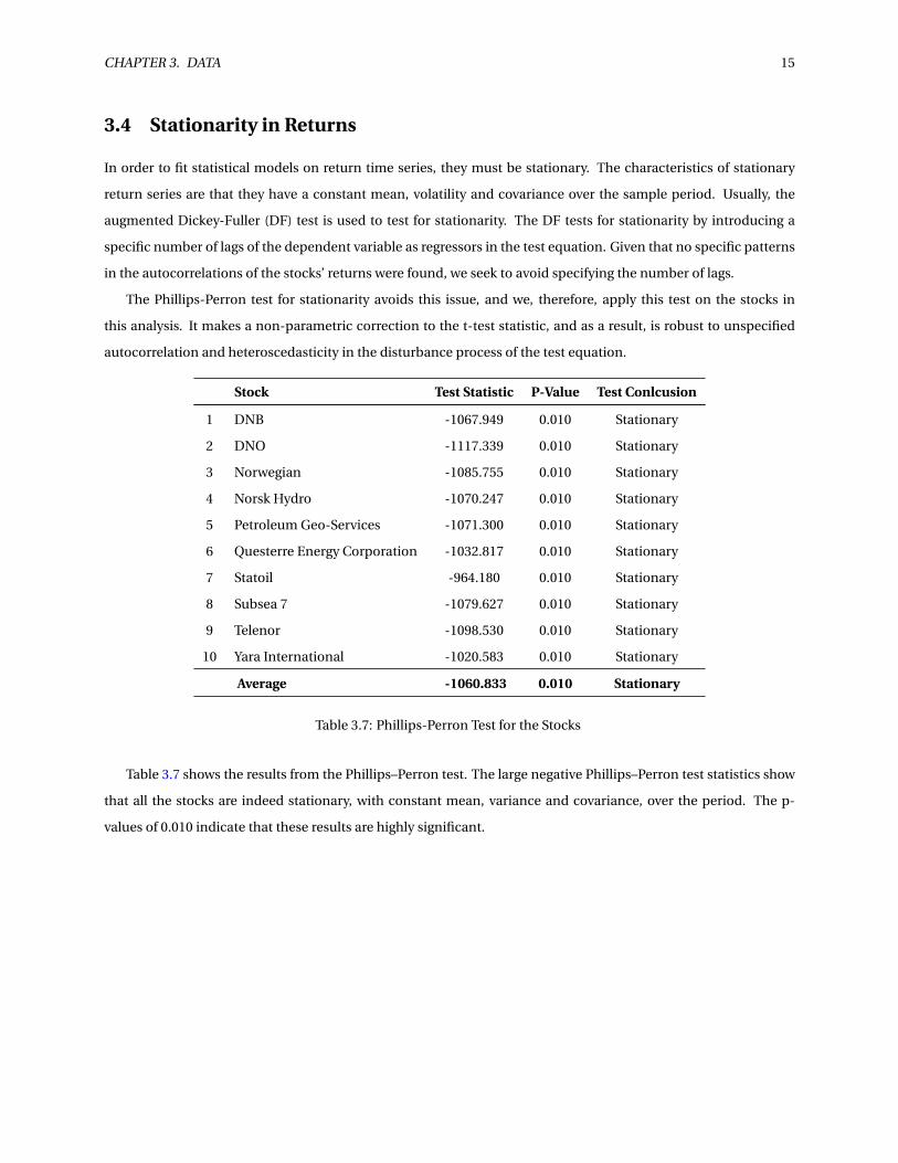
3.4 Stationarity in Returns

In order to fit statistical models on return time series, they must be stationary. The characteristics of stationary

return series are that they have a constant mean, volatility and covariance over the sample period. Usually, the

augmented Dickey-Fuller (DF) test is used to test for stationarity. The DF tests for stationarity by introducing a

specific number of lags of the dependent variable as regressors in the test equation. Given that no specific patterns

in the autocorrelations of the stocks’ returns were found, we seek to avoid specifying the number of lags.

The Phillips-Perron test for stationarity avoids this issue, and we, therefore, apply this test on the stocks in

this analysis. It makes a non-parametric correction to the t-test statistic, and as a result, is robust to unspecified

autocorrelation and heteroscedasticity in the disturbance process of the test equation.

Stock Test Statistic P-Value Test Conlcusion

1 DNB -1067.949 0.010 Stationary

2 DNO -1117.339 0.010 Stationary

3 Norwegian -1085.755 0.010 Stationary

4 Norsk Hydro -1070.247 0.010 Stationary

5 Petroleum Geo-Services -1071.300 0.010 Stationary

6 Questerre Energy Corporation -1032.817 0.010 Stationary

7 Statoil -964.180 0.010 Stationary

8 Subsea 7 -1079.627 0.010 Stationary

9 Telenor -1098.530 0.010 Stationary

10 Yara International -1020.583 0.010 Stationary

Average -1060.833 0.010 Stationary

Table 3.7: Phillips-Perron Test for the Stocks

Table 3.7 shows the results from the Phillips–Perron test. The large negative Phillips–Perron test statistics show

that all the stocks are indeed stationary, with constant mean, variance and covariance, over the period. The p-

values of 0.010 indicate that these results are highly significant.

4. Methodology

The methodology of our analysis is structured with three main components. First, we present a theoretical back-

ground of stock returns, the ARMA-GARCH forecasting model and parameter estimation. Second, we discuss our

implementation of a dynamic ARMA(w,x)-(g)GARCH(1,1)-(M) model, the parameters used and our approach for

model fitting. Lastly, the forecasting model assessment framework is described, divided into statistical properties,

return generating properties and a review of the model’s computational complexity.

The forecasting model is centred around seven sets that are input parameters to our forecasting model. These

sets will be referred to throughout the methodology section, and are displayed in Table 4.2.

Sets

Stocks, I

{DNB (DNB), DNO (DNO), Norsk Hydro (NHY), Norwegian (NAS),

Petroleum Geo-Services (PGS), Questerre Energy Corporation (QEC)

Statoil (STL), Subsea 7 (SUBC), Telenor (TEL), Yara International (YAR)}

Sample sizes, S{500, 1000

}Days, T

{1, ..., 1072

}

Distributions, D

{Normal Distribution (NORM), Generalized Error Distribution (GED),

Student t Distribution (STD), Skewed Normal Distribution (SNORM),

Skewed Generalised Error Distribution (SGED), Skewed Student t Distribution (SSTD),

Generalized Hyperbolic Function Distribution (GHYP), Generalized Hyperbolic Skewed Student t-

Distribution, Skewed Generalised Error Distribution (SGED),

Normal Inverse Gaussian Distribution (NIG)}

GARCH models, G{S, GJR, E

}AR-lags, W

{0, ..., 6

}MA-lags, X

{0, ..., 6

}In-Mean, M

{TRUE, FALSE

}

Table 4.2: Sets of Input Parameters To the Forecasting Model

16

CHAPTER 4. METHODOLOGY 17

4.1 Theoretical Background of the ARMA-GARCH Forecasting Model

This section serves as an introduction to the ARMA-GARCH forecasting model, which is commonly used by finan-

cial institutions to model return and volatility of financial assets. One of the most general models for modelling the

returns of financial assets, combines a stationary, moving-average error process with a stationary, autoregressive

representation. We will name this the autoregressive moving average (ARMA) representation of a return series.

Further, the generalised autoregressive conditional heteroscedasticity (GARCH) is specifically designed to model

the volatility of financial assets. The GARCH model is made up of two equations: the conditional mean and the con-

ditional variance equation. By representing the conditional mean equation as an ARMA process, we can combine

the two concepts, ARMA and GARCH, obtaining an ARMA-GARCH that can be used for forecasting returns.

To further understand the ARMA-GARCH model, we must clarify the distinction between the unconditional

mean and variance and the conditional mean and variance of a time series of returns. The unconditional mean

and variance are merely the mean and variance of the returns distribution, which are assumed constant over the

entire period considered. It can be thought of as the long-term average mean and variance over that period. For

instance, if the model is the simple "returns are independent and identically distributed (i.i.d.)" model, we can

disregard the ordering of the returns in the sample and just estimate the sample mean and variance.

On the other hand, the conditional mean and conditional variance will change at every point in time. The

conditional mean and conditional variance depend on the history of returns up to that point. That is, we account

for the dynamic properties of returns by regarding their distribution at any point in time as being conditional on all

the information up to that point. The forecasts made from the ARMA-GARCH models are not equal to the current

estimates. Instead, return and volatility forecasts can be higher or lower than the average over the short term, but as

the forecast horizon increases the return and volatility forecasts converge to the long-term, unconditional volatility.

The distribution of a return at time t , regards all the past returns up to and including time t −1 as being non-

stochastic. We denote the information set, which is the set containing all the past returns up to and including time

t −1, by It−1. The information set contains all the prices and returns that we can observe.

We write rt to denote the conditional mean and σ2t to denote the conditional variance at time t . This corre-

sponds to the mean and variance at time t , conditional on the information set. When the distribution of returns at

every point in time is normal, we write:

rt |It−1 ∼ N (rt ,σ2t ) (4.1)

4.1.1 Return Distributions

The return distribution is an important assumption of the ARMA-GARCH model. Most commonly, the normal

distribution is assumed, but as financial time series often exhibit leptokurtosis and skewness, other distributions

may be more appropriate.


Volatility clustering can explain why the distribution of daily returns is not normal. If returns exhibit volatility

clustering, the return series is obtained from a mixture distribution. When this is the case, the kurtosis exceeds the

normal kurtosis of three. In addition, the skew is greater or less than zero. As shown in the last two columns in Table

3.2, this is the case for all of the stocks we consider. As a result, the return distribution will likely exhibit high peaks,

fat tails and/or skewness compared to a normal return distribution. To account for these finding, we will assume

that the return series of stock i , is distributed according to one of the distributions d , in Table 4.2. As a result, we

write:

ri ,t |Ii ,t−1 ∼ d(ri ,t ,σ2i ,t ), d ∈ D (4.2)

For a parametric model to adequately describe the properties of a distribution, it must have at least four param-

eters: a location and scale parameter, also known as mean and variance, respectively, in addition to a parameter

describing the decay of the tails and an asymmetry parameter. The asymmetry parameter allows the left and right

tails to have different behaviour. The more parameters a model consists of, the more complex the model is. For

instance, the skewed generalised error distribution has all the four parameters, while the normal distribution only

has the mean and variance parameters.

However, there is a trade-off between the goodness of fit and the number of parameters in the model. In order

to avoid overfitting and to evaluate which of the given distributions are the best fit for a given return series, we apply

the Akaike information criterion (AIC). In general terms, the AIC is an estimator of the relative quality of statistical

models for a given set of data. Given a collection of models for the data, the AIC estimates the quality of each model,

relative to each of the other models. Thus, the AIC provides means for the model selection.

Let k be the number of estimated parameters in the model and L be the maximum value of the likelihood

function for the model. Then the AIC value of the model is given by the following formula:

AIC = 2k −2ln(L) (4.3)

4.1.2 The Conditional Mean Equation

The conditional mean equation specifies the behaviour of the returns. The conditional mean equation of a GARCH

model can take several forms, and in this thesis, we will assume that the return series follows an autoregressive

moving average, ARMA, model developed by Box and Jenkins (46). The ARMA accounts for the possibility of returns

being autocorrelated and to be dependent on the previous error terms. Hence, the conditional mean equation will

take the following form:

ri ,t = ci +w∑

j=1κi , j ri ,t− j +

x∑j=1

µi , j εi ,t− j +εi ,t , ∀t ∈ T, ∀i ∈ I , εi ,t |Ii ,t−1 ∼ d(0,σ2i ), d ∈ D (4.4)

where ci is the constant term, ri ,t is the observed realized return at time t , κi , j is the autoregressive constant, εi ,t− j

is the realized error at time t , µi , j is the moving average coefficient and εi ,t the white noise. Note that we allow


the innovations, εi ,t , to be drawn from any of the distributions in the set D . The w and x describe the number of

autoregressive and moving average terms, respectively.

4.1.3 The Conditional Variance Equation

The GARCH model was introduced by Bollerslev (7), which is a generalisation of the ARCH model, originally de-

veloped by Engle (8). The ARCH model allows for many lags in the conditional variance, and the GARCH model

extends it by also allowing for lags in the error terms. Note that the GARCH model can be expressed in a form show-

ing it is effectively an ARMA model for the conditional variance, which is why GARCH is used to model time-varying

volatility where the volatility is clustered. Keep in mind that we showed in the last chapter, that the stocks in our

study exhibit volatility clustering. The GARCH(y ,z) has the conditional volatility equation given by:

σ2i ,t =ωi +

y∑j=1

αi , j ε2i ,t− j +

z∑j=1

βi , jσ2i ,t− j , ∀t ∈ T, ∀i ∈ I , εi ,t |Ii ,t−1 ∼ d(0,σ2

i ,t ), d ∈ D (4.5)

where ωi is the constant term, ε2i ,t− j is the squared error term at time t , αi , j is the associated constant, σ2

i ,t− j is the

lagged conditional variance at time t and βi , j is the autoregressive constant. Note that we allow the innovations,

εi ,t , to be drawn from any of the distributions in the set D . The y and z describe the number of lags for the error

term and lags for the conditional variance, respectively.

The GARCH error parameter, α, measures the reaction of the conditional volatility to market shocks. When α is

relatively large, above 0.1, the volatility is very sensitive to market shocks. The GARCH lag parameter, β, measures

the persistence in conditional volatility, irrespective of anything happening in the market. When β is relatively

large, above 0.9, the volatility takes a long time to die out. The sum α+β determines the rate of convergence of the

conditional volatility to the long-term average level.

4.1.4 The Unconditional Variance of GARCH(y ,z)

In the absence of market shocks, the GARCH conditional variance will eventually settle to a steady-state value.

This is the value σ2, such that σ2t = σ2, for all t. We define σ2 the unconditional variance of the GARCH model,

corresponding to a long-term average value of the conditional variance. The theoretical value of the GARCH long-

term or unconditional variance is not the same as the unconditional variance in a moving-average volatility model.

The moving average unconditional variance is called the i.i.d. variance, because it is based on the i.i.d. returns

assumption. The theoretical value of the unconditional variance in a GARCH model is clearly not based on the

i.i.d. returns assumption. The long-term or unconditional variance is found by substituting σ2t = σ2

t−1 = σ2 into

the GARCH conditional variance equation, equation 4.5. We also use the fact that E(ε2t−1) = σ2

t−1. This yields the


following formula for the long-term variance of the GARCH model:

σ2i =

ωi

1− (∑y

j=1αi , j +∑zj=1βi , j )

, ∀i ∈ I (4.6)

4.1.5 ARMA-GARCH Model Formulations

GARCH models have several extensions to account for effects not captured in the regular symmetric GARCH (S-

GARCH). We will now present the formulations of the S-GARCH, in addition to the two model extensions explored

in this study: the exponential GARCH (E-GARCH) and the Glosten-Jagannathan-Runkle GARCH (GJR-GARCH).

All have their conditional mean equation modified as an ARMA process. Also, we present the inclusion of the

conditional volatility in the conditional mean equation to obtain a GARCH-M model, for the GJR-GARCH and the

E-GARCH. We define all models in terms of days, sample sizes and stocks, which are entirely defined in Table 4.2.

For clarification, the sample size is the number of observations used to estimate the parameters of the ARMA-

GARCH forecasting model.

ARMA(w, x)-S-GARCH(1,1)

The symmetric GARCH model, the S-GARCH, was introduced by Bollerslev (7), and is the plain vanilla version of

the GARCH models. The conditional mean equation follows an ARMA process, as introduced in equation 4.4. The

conditional variance equation is equal to equation 4.5, but the lags are now restricted to only one. Note that we

allow the innovations, εi ,t , to be drawn from any of the distributions in the set D . The ARMA(w, x)-S-GARCH(1,1)

model is given by the following expressions:

ri ,t = ci ,s,t +w∑

j=1κi ,s, j ri ,t− j +

x∑j=1

µi ,s, j εi ,s,t− j +εi ,s,t , ∀i ∈ I ,∀s ∈ S,∀t ∈ T (4.7)

σ2i ,t =ωi ,s,t +αi ,s,tε

2i ,s,t−1 +βi ,s,tσ

2i ,t−1, ∀i ∈ I ,∀s ∈ S,∀t ∈ T εi ,s,t |Ii ,t−1 ∼ d(0,σ2

i ,t ), d ∈ D (4.8)

ARMA(w, x)-GJR-GARCH(1,1)-M

In order to capture the leverage effect, Glosten et al. (26) introduced the GJR-GARCH. The model includes a single

extra leverage parameter in the conditional variance equation. This extra parameter is formulated such that the

asymmetric response is only augmented from negative market shocks, using an indicator function. Further, the

conditional mean equation from equation 4.4 is now enhanced by including the conditional volatility term, to

model volatility feedback. Collectively, we obtain the ARMA(w, x)-GJR-GARCH(1,1)-M model, represented by the

following expressions:




x∑j=1

µi ,s, j εi ,s,t− j +ηi ,s,tσi ,t +εi ,s,t , ∀i ∈ I ,∀s ∈ S,∀t ∈ T (4.9)

σ2i ,t =ωi ,s,t +αi ,s,tε

2i ,s,t−1 +λ1{εi ,s,t−1<0}ε

2i ,s,t−1 +βi ,s,tσ

2i ,t−1, ∀i ∈ I ,∀s ∈ S,∀t ∈ T εi ,s,t |Ii ,t−1 ∼ d(0,σ2

i ,t ), d ∈ D

(4.10)

where λ captures the leverage effect when the indicator function, 1{εt−1<0}, is activated. η is the parameter account-

ing for the volatility feedback.

ARMA(w, x)-E-GARCH(1,1)-M

The E-GARCH model developed by Nelson (24), addresses the problem of ensuring positive and finite variance by

formulating the conditional variance equation in terms of the log of the variance. The standard specification of the

conditional variance equation is given by:

l n(λ2t ) =ω+ g (zt−1)+βl n(λ2

t−1), zt |It−1 ∼ d(0,σ2), d ∈ D (4.11)

where zt is a realisation of Zt , a random variable distributed according to one of the distributions in D . g (zt−1) =θzt +γ

(|zt |−E(|Zt |))

is an asymmetric response function enabling reactions to market shocks, including only pos-

itive or only negative.

The conditional mean equation takes the same form as in the ARMA(w, x)-GJR-GARCH(1,1)-M. Thus, the ARMA(w, x)-

E-GARCH(1,1)-M is defined by the following set of equations:



x∑j=1

µi ,s, j εi ,s,t− j +ηi ,s,tσi ,t +εi ,s,t , ∀i ∈ I ,∀s ∈ S,∀t ∈ T (4.12)

ln(λ2i ,t ) =ωi ,s,t + g (zi ,t−1)+βi ,s,t ln(λ2

i ,t−1), ∀i ∈ I ,∀s ∈ S,∀t ∈ T εi ,s,t |Ii ,t−1 ∼ d(0,σ2i ,t ), d ∈ D (4.13)

4.1.6 Parameter Estimation

Having introduced the various ARMA-GARCH model formulations, we are now ready to explain how the parameters

of the models are estimated. By maximising the value of the log-likelihood function, one can estimate the optimal

values of the given parameters.

Given that we have introduced three different ARMA-GARCH formulations, we will for simplicity use the ARMA-

S-GARCH specification to show the maximum likelihood (ML) derivations. Assuming that the error process is nor-

mally distributed, we now introduce the log-likelihood function of the ARMA(w, x)-S-GARCH(y, z). Before we cal-

culate the log-likelihood function of the ARMA(w, x)-S-GARCH(y, z), we show the log-likelihood function of the

plain vanilla ARMA(w, x).


ML estimation of the ARMA(w, x)

In the case of ML estimation of the plain vanilla ARMA, where σ2t = σ2, maximizing the normal log likelihood re-

duces to the problem of maximizing:

l n(Li ,t ) =−1

2

T∑t=1

(ln(σ2

i )+ (εi ,t

σi)2

)(4.14)

with respect to all the parameters. To do this, we solve the conditional mean equation (4.4) for εt :

εi ,t = ri ,t −w∑

j=1κi , j ri ,t− j −

x∑j=1

µi , j εi ,t− j − ci (4.15)

Finally we insert the above equation (4.15) and the conditional volatility equation (4.5) into the ML function (4.14):

l n(Li ,t ) =−1

2

T∑t=1

(ln(σ2

i )+( (ri ,t −∑w

j=1κi , j ri ,t− j −∑xj=1µi , j εi ,t− j − ci )2

σ2i

))(4.16)

ML Estimation of the ARMA(w, x)-S-GARCH(y, z)

By adding the conditional variance equation, noting that the volatility now is time-varying, the problem of max-

imising the normal likelihood reduces to:

ln(Li ,t ) =−1

2

T∑t=1

(l n(σ2

i ,t )+ (εi ,t

σi ,t)2

)(4.17)

with respect to all the parameters. The conditional mean equation is solved for epsilon, just as in equation 4.15,

and together with the conditional volatility equation (4.5), inserted into the maximum likelihood function (4.17):

ln(Li ,t ) =−1

2

T∑t=1

(l n

(ωi +

y∑j=1

αi , j ε2i ,t− j +

z∑j=1

βi , jσ2i ,t− j

)+ ( (ri ,t −∑wj=1κi , j ri ,t− j −∑x

j=1µi , j εi ,t− j − ci )2

ωi +∑yj=1αi , j ε

2i ,t− j +

∑zj=1βi , jσ

2i ,t− j

))(4.18)

This expression is now optimized to obtain the optimal parameter values, for the given data, given by the following

parameter constraints:

ωi > 0, αi , j ,βi , j ≥ 0 ∀ j ,y∑

j=1αi , j +

z∑j=1

βi , j < 1 (4.19)

Likewise, the ML function can be derived for both the ARMA(w, x)-GJR-GARCH(y, z)-M and ARMA(w, x)-E-

GARCH(y, z)-M, with all the distributions in set D.


4.2 Implementation of a Dynamical ARMA(w, x)-(g )GARCH(1,1)-(M) Fore-

casting Model

In the last section, Section 4.1, we introduced the various components constituting our return forecasting model.

This section gives an in-depth overview of the actual implementation of the dynamic ARMA(w, x)-(g )GARCH(1,1)-

(M) forecasting model. Firstly, we present a complete overview of the implementation, both from a flowchart and

more descriptive text. This process spans the fitting and forecasting processes, from selecting a stock until the

one-day-ahead return and volatility forecasts are obtained. Secondly, we provide a model assessment framework,

including statistical properties, return-generating properties and a review of the model’s computational complex-

ity.

Figure 4.1: Flowchart of the Forecasting Model


4.2.1 Model Implementation Overview

Figure 4.1 illustrates how our implementation is structured. We systematically test for different combinations for

the values of the input parameters, to obtain the best fitted ARMA(w, x)-(g )GARCH(1,1)-(M) forecasting model.

For each combination of input parameters, the forecasting model returns three values: an AIC describing the fit of

the model, and the one-day-ahead return and volatility forecasts.

4.2.2 The Dynamic Properties of the Forecasting Model

Following our implementation, one optimal ARMA(w, x)-(g )GARCH(1,1)-(M) forecasting model is fitted, based on

the combinations described in Figure 4.1, using a rolling window approach. This model then produces the out-

of-sample, one-day-ahead return and volatility forecasts. Because the model uses a rolling window approach, for

each sample size s, the last s daily data points are used as the sample window. Moreover, the start date, t = 1, in the

rolling window is fixed by the largest sample size, because we want to evaluate the forecasting performance across

sample sizes from the same date. The period considered ranges from January 2010 to April 2018, containing 2072

daily data points. As a result, the forecasting model rolls over 2072−max(500,1000) = 1072 days. The process is

illustrated in Figure 4.2, with four iterations in the outer loop, with sample size 500. The outer loop is shown in

Figure 4.1.

Figure 4.2: Rolling Window Illustration


For a given combination of stock i , sample size s, and day t , in the rolling window, referred to as an iteration

of the outer loop, we want to choose the input parameters that result in the best forecasting model fit and use that

model to obtain return and volatility forecasts. In other words, we have to test which values of d , g , w and x will

result in the best model fit for each iteration of the outer loop. Testing one combination of g , w and x is referred

to as one iteration of the inner loop. First, for a given iteration of the outer loop, the distribution d , giving the best

fit to the given sample window is obtained. Then, we use a brute force approach where we test all combinations

of g , w and s, along with the best fitted distribution, d , found in the previous step, as input parameters to the

ARMA(w, x)-(g )GARCH(1,1)-(M) forecasting model. Only when using the GJR-GARCH or E-GARCH models, the

conditional volatility is added as a component to the conditional mean equation, implying that M = T RU E .

The ARMA(w, x)-(g )GARCH(1,1)-(M) output parameters, the forecasts and maximum likelihood estimates, are

calculated for each iteration of the inner loop. The best fitting model is chosen based on the lowest Akaike infor-

mation criterion (AIC). The AIC is an estimator of the relative quality of statistical models for a given set of data.

Given a collection of models for the data, the AIC estimates the quality of each model, relative to each of the other

models. Thus, the AIC provides a means for model selection among all iterations of the inner loop, for one iteration

of the outer loop. The AIC of a given model is calculated using the following equation:

AICi ,s,t = 2ki ,s −2l n(Li ,s,t ), ∀i ∈ I ,∀s ∈ S,∀t ∈ T (4.20)

where k is the number of estimated parameters and L is the maximum value of the likelihood function. In addition,

i is stock, s is the sample size and t is the day.

4.2.3 Obtaining Forecasts From the Forecasting Model

The model with the lowest AIC has the optimal combination of input parameters. This provides the optimal

ARMA(w, x)-(g )GARCH(1,1)-(M) output parameters, which can be used to calculate the optimal return and volatil-

ity forecasts, for a given iteration in the outer loop. After the ARMA(w, x)-(g )GARCH(1,1)-(M) forecasting model is

fitted across the rolling window, we have obtained the optimal out-of-sample, one-day-ahead return and volatility

forecasts for each stock, for each sample size, for each day.

Calculating the Out-Of-Sample, One-Day-Ahead Return and Volatility Forecasts

Let us assume that the optimal input parameters, the input parameters that gives the best model fit for a given

iteration in the outer loop, results in a plain vanilla ARMA(w, x)-S-GARCH(1,1) forecasting model. The out-of-

sample, one-day-ahead return forecast of a given stock i , sample size s, and day t , is calculated by taking the

expectation of the conditional mean equation 4.7, introduced in the previous section:

E(ri ,s,t ) = ci ,s +w∑


w∑j=1

µi ,s, j εi ,s,t− j , ∀s ∈ S, ∀i ∈ I , ∀t ∈ T (4.21)


The expectation of the error process, εt , is assumed to be zero. Today’s optimal output parameters is the best guess

on what the optimal output parameters would be tomorrow. Hence, the optimal output parameters at time t is

used to forecast the return at time t +1. Using equation 4.21, our return forecast at time t for time t +1 for a given

stock i , with sample size s, is:

E(ri ,s,t+1) = ci ,s +w∑


x∑j=0

µi ,s, j εi ,s,t− j , ∀s ∈ S, ∀i ∈ I , ∀t ∈ T (4.22)

Holding on to our assumptions and using the same approach as above, the out-of-sample, one-day-ahead

volatility forecast of a given stock i , sample size s, and day t , is calculated by first taking the expectation of the

conditional variance equation, 4.7:

E(σi ,s,t ) =√√√√ωi ,s +

y∑j=1

αi ,s, j ε2i ,s,t− j +

z∑j=1

βi ,s, jσ2i ,t− j , ∀s ∈ S, ∀i ∈ I , ∀t ∈ T (4.23)

Using equation 4.23, we move one time step forward and use the optimal output parameters at time t to forecast

the volatility at time t +1:

E(σi ,s,t+1) =√√√√ωi ,s +

y∑j=0

αi ,s, j ε2i ,s,t− j +

z∑j=0

βi ,s, jσ2i ,t− j , ∀s ∈ S, ∀i ∈ I , ∀t ∈ T (4.24)

4.3 Forecasting Model Assessment Framework

We have now described the implementation of the dynamic forecasting model. In this section, we present our ap-

proach to evaluate the model’s return forecasting performance in terms of both statistical and economical metrics,

as well as a discussion of the model’s computational complexity.

4.3.1 Statistical Properties

The ARMA-GARCH model produces a series of out-of-sample, one-day-ahead return forecasts. We calculate the

return forecasting error for each day t , stock i , and sample size s, over the rolling window, as:

εfi ,s,t = r r

i ,s,t − r ei ,s,t , ∀i ∈ I , ∀s ∈ S, ∀t ∈ T (4.25)

where ε fi ,s,t is the return forecasting error, the difference between the realized return r r

i ,s,t , and the return forecasting

estimate r ei ,s,t , for a given stock i , sample size s and day t . In order to assess the return forecasting accuracy and

precision, we now define two statistical metrics.


Mean Absolute Error (MAE)

Firstly, as a statistical measure of forecasting accuracy for a given stock i , with sample size s, we define the mean

absolute error (MAE). That is the average absolute forecast error for a given stock, and the mathematical expression

is given by:

M AEi ,s = 1

|T |T∑

t=1

∣∣r ri ,s,t − r e

i ,s,t

∣∣, ∀s ∈ S, ∀i ∈ I (4.26)

where s is the sample size and i is the given stock.

Standard Deviation of the Absolute Error

Secondly, as a statistical measure of forecasting precision for a given stock i , and sample size s, we define the

standard deviation of the absolute error. The mathematical expression is given by:

σAE ,i ,s =√√√√ 1

|T |T∑

t=1

(∣∣r ri ,s,t − r e

i ,s,t

∣∣−M AEi ,s

)2, ∀s ∈ S, ∀i ∈ I (4.27)

where s is the sample size and i is the given stock.

Hit Ratio

As a measure of the market timing ability of the return forecasting model, we define the hit ratio. This ratio is

calculated as the proportion of days the model correctly predicts the direction of the out-of-sample, one-day-ahead

return, for a given stock i , and sample size s:

Hit ratioi ,s =Correct Out-of-Sample, One-Day-Ahead Directional Predictionsi ,s

|T | , ∀s ∈ S, ∀i ∈ I (4.28)

where i is stock and s is the sample size. As an example, assume the model forecasts a positive out-of-sample,

one-day-ahead return and the realised return is positive. Then this forecast will be recorded as a hit. Contrary, if

the realised return is negative, the prediction will be recorded as a miss.

4.3.2 Return Generating Properties

We will now present the short-long strategy and the bound strategy, two trading strategies used to indicate the

profitability of trading according to the forecasting model. In addition, we present the buy-and-hold strategy as a

benchmark for comparison. These strategies are explained in detail below.

Further, to create a realistic trading scenario, we have considered the strategies with transaction costs for each

trade executed. We have assumed that the transaction cost is a percentage fee in commissions to the broker. As we


are considering liquid stocks from the OBX, we have chosen to neglect the indirect trading cost incurred from the

bid/ask spread and potential price impact.

We have assumed a percentage transaction fee of 10 bps for each trade made, following the average commission

rates paid by institutional investors on global equity trades (41). If a trade is made, the fee will be subtracted from

the daily return obtained. Note that the fee is applied to both buying and short selling the stocks. If the model

prediction requires a shift in position, for instance from long to short, this will require two trades, and subsequently,

two fees will be subtracted from the daily return.

In reality, the cost of short selling is greater than the cost of buying, as you would need to pay a loan fee over the

shorting period. This loan fee will also be dependent on the stock, as the availability of borrowing the stock from

current shareholders influences the cost of shorting. Due to the lack of transparency and availability of information

on these fees, we have not included this shorting cost in our model.

Lastly, we assume 250 trading days per year, and this will be used to annualise the accumulated return and

alpha metrics.

Buy-and-Hold Strategy

The buy-and-hold strategy is executed by holding a stock from the start to the end of the rolling window. The annu-

alised return obtained from following a buy-and-hold strategy is defined as rB H . We also define the average, daily

return as µB H and the daily standard deviation as σB H . This strategy will be used as a benchmark for measuring

the success of the strategies described below.

Short-Long Strategy

The short-long strategy is executed to assess the profitability of following the out-of-sample, one-day-ahead return

predictions of the forecasting model, and comparing it to a common buy-and-hold strategy. We define the short-

long strategy, with its associated annualised return as rSL , the average, daily return as µSL and the daily standard

deviation as σSL .

The short-long return is defined as the annualised return from trading according to the out-of-sample, one-

day-ahead return predictions of the forecasting model from the start to the end of the rolling window. Following

the short-long strategy implies actively deciding on a new position in every stock, each day. The short-long strategy

will take a long position if the forecasting model predicts a positive return, and a short position if the forecasting

model predicts a negative return for the next day. The return for a stock, a given day, is calculated as follows: if the

model predicts the correct direction of the out-of-sample, one-day-ahead realised return, the absolute value of the

realised return is added to the current accumulated return. Likewise, if the model predicts the wrong direction, the

absolute value of the realised return is subtracted from the current accumulated return.


Bound Strategy

As the short-long strategy will most likely make a significant amount of trades, and thereby reduce the return when

considering transaction costs, we will try a new trading strategy, the bound strategy. The bound strategy aims to

reduce the number of trades, by discarding forecasting noise and only trade when the return forecasting model

signals larger market shocks. In other words, the strategy only makes a trade when the forecasts are above some

degree of certainty.

The bound strategy is executed to assess the model’s ability to predict the significant deviations in returns, the

more substantial market shocks. We define the trading bound, measured as a percentage of the GARCH’s out-of-

sample, one-day-ahead volatility forecast, obtained from the currently fitted ARMA-GARCH model. The trading

bounds used in this study are 0.5σ and 0.35σ, with the sample size 500 and 1000, respectively. The reason for

choosing these specific trading bounds will become clear in Chapter 5, Results.

The trading strategy is configured to take a long or short position if the absolute value of the out-of-sample, one-

day-ahead return forecast is above or below the trading bound, respectively, given that there is no current active

position. If the forecasting model is in a long position and the out-of-sample, one-day-ahead forecast is positive,

the position is held. If the out-of-sample, one-day-ahead forecast is negative, but not below the trading bound,

the position is sold and no new active position is taken. However, if the out-of-sample, one-day-ahead forecast is

negative and below the trading bound, a short position is engaged. This argument is similar if the starting position

is short.

We define the bound strategy, with its associated bound return, as rBound . It is defined as the annualised return

from trading according to the strategy from the start to the end of the period. In addition, we define the bound

strategy’s average, daily return as µBound and the daily standard deviation as σBound .

Alpha

We define alpha, α, as the difference rSL − rB H and rBound − rB H , respectively. Hence, this is the annualised, excess

return from following the given strategy compared to the buy-and-hold strategy. The alpha is a widely adopted

metric in the financial industry for measuring the performance of active investment strategies and will give a strong

indication of the success of the forecasting model.

Sharpe Ratio

Finally, we define the Sharpe ratio of the buy-and-hold, short-long and bound strategies. It is a metric for measuring

the risk-adjusted abnormal returns of a stock or portfolio. The Sharpe ratio is defined as the excess return over the

risk-free rate, divided by the standard deviation. We annualise the daily µB H , r f and σB H by multiplying by the


number of trading days per year, 250. Hence, we obtain the following three Sharpe ratios:

SB H =p250

µB H − r f

σB H(4.29)

SSL =p250

µSL − r f

σSL(4.30)

SBound =p250

µBound − r f

σBound(4.31)

4.3.3 Computational Complexity and Run Time Properties

The computation time used to fit the optimal forecasting model is crucial for the applicability of the forecasting

model. Given the comprehensive forecasting model fitting process with several sets (Table 4.2) of input parameters,

we have been forced to write efficient R code and carefully consider the convergence properties of the ARMA(w, x)-

(g )GARCH(1,1)-(M) forecasting model for different input combinations.

The forecasting model setup, with a variety of input parameter combinations, requires an exponential number

of ML calculations. As a consequence, we were granted access to the calculation cluster Solstorm, belonging to

the Department of Industrial Economics and Technology Management at NTNU. The programming was done in

R, and below is, therefore, a description of the software and key R libraries we utilised, in addition to the hardware

capabilities of the node used on the Solstorm calculation cluster.

Processor 4x 2.2GHz AMD Opteron 6274 – 16 core

Memory 128Gb RAM

Disk 300Gb SAS 15k rpm

R version R.3.4.4

Key R libraries rugarch, paralell, doParalell, sys, R.util

Table 4.3: Hardware and Software Used in Testing

To speed up the calculations and reduce the runtime, we were able to run one outer loop on each of the 64 cores

available per node. That is, for a given stock i , sample size s, and day t , we assigned this process to its own core,

to calculate all the iterations of the inner loop. Having 64 cores at our disposal, we could iterate through the outer

loop in batches of 64 days at a time. This was done utilising the parallel and doParallel packages in R. Moreover, in

order to apply an upper bound on the total time spent on demanding activities, we employed a timeout function,

functionality provided with the R library sys and R.Util. This ensured us that combinations of variables that did not

converge when fitting the underlying return distribution or ARMA(w, x)-(g )GARCH(1,1)-(M) forecasting model,

was timed out and the program would move to the next iteration of the inner loop. The timeout functionality

drastically reduced the runtime. The total run time for this study was over nine days.

In addition to the vast number of models to test for each stock and sample size, each day, the aspect of ML

convergence was a time-consuming activity. In particular, ML optimisation with the conditional volatility in the


conditional mean equation, the choice of sample size and the fitting of complex distributions were three critical

issues we wish to highlight.

Complexity of ML Optimization for ARMA-GARCH-M

The inclusion of the conditional volatility in the conditional mean equation raised some computational issues. The

parameters of both the conditional mean equation and conditional variance equation must be estimated together,

by ML optimisation. The maximisation of the likelihood function becomes somewhat complex, as the first deriva-

tives of the likelihood must be recursively or numerically computed (47). This drastically increased the run time of

the program.

Sample Properties and Convergence Issues of the GARCH Model

Optimization of GARCH(1,1) models using maximum likelihood has shown to be numerically challenging to com-

pute, and models may not converge (39). The sample size proved to be a pivotal variable to ensure convergence.

Hwang et al. (40) conducted a comprehensive study on small sample properties of GARCH estimates and

persistence. Results show that Bollerslev’s non-negativity conditions are critical restrictions in small samples for

GARCH(1,1), causing a severe number of convergence errors. Also, their findings show that the GARCH parame-

ters tend to be downward biased. They propose that at least 500 observations for GARCH(1,1) models are used,

given biases and convergence error. In our study, we have experienced problems using smaller samples sizes and

therefore ended up employing two sample sizes of 500 and 1000.

Convergence Issues of Complex Distributions

In our experience, the use of complex distributions, such as normal inverse Gaussian distribution and generalised

hyperbolic skew student t distribution, gave the ML optimisation difficulties of converging. The reason is that these

distributions together can capture both return characteristics such as skewness and leptokurtosis, and such have

more parameters to optimise in the ML optimisation.

Collectively, the computational issues described above has forced us to restrict the scope of our study to in-

clude fewer stocks, a shorter time horizon and fewer sample sizes than desirable. However, our selection of these

variables was made after comprehensive testing, to ensure a broad enough testing environment.

5. Results

The results section is structured in two parts. First, we will give a brief description of the characteristics and the

dynamic behaviour of the ARMA-GARCH forecasting model, both over time and across the stocks. Second, we

evaluate the return forecasting performance in terms of statistical metrics and return generating properties.

5.1 Model Characteristics

To provide an overview of the characteristics and dynamic behaviour of the ARMA-GARCH forecasting model, we

will investigate the distribution of the fitted GARCH models and the average fitted AR lags and MA lags, both over

time and across the stocks. Also, we will present the most fitted underlying return distribution for each stock. First,

we discuss the model characteristics over time, before we compare the model characteristics between the stocks.

5.1.1 Model Characteristics Over Time

Plots 5.1a and 5.1b show the distribution of the fitted GARCH models for the stocks, for each time step over the

rolling window, with sample size 500 and 1000, respectively. Also, in the lower section of the plot, is the squared

returns of the OBX, as an indicator of the current market condition.

There is a trend that the E-GARCH-M is the dominant model, irrespective of the market condition. The GJR-

GARCH-M is a good fit, while the symmetric S-GARCH is the least fitted model, consistent with the findings of

Erdem et al. (31). Looking at plot 5.1b, we see that the E-GARCH-M becomes an even more fitted model as the

sample size increases.

Moreover, the impact from the inclusion of the conditional volatility in the conditional mean equation is note-

worthy. As both the E-GARCH-M and GJR-GARCH-M outperform the S-GARCH in terms of fit, one could argue that

the in-mean modification is important for stock return modelling, as also argued by Hansson and Hördahl (27) and

Liu et al. (30). However, as there were no E-GARCH or GJR-GARCH without the in-mean term, in this analysis, the

total impact of the volatility feedback is hard to determine.

Collectively, results indicate that asymmetric GARCH models, accounting for the leverage effect and volatility

feedback, is suitable to model stock returns compared to the S-GARCH. It is also worth noting that the E-GARCH-

M is preferred over the GJR-GARCH-M. A reason may be the E-GARCH-M’s approach to avoid the non-negativity

constraints, and thus make ML convergence more likely.

32

CH

AP

TE

R5.

RE

SULT

S33

(a) Sample Size 500 (b) Sample Size 1000

Figure 5.1: Distribution of Fitted GARCH Models and OBX Squared Returns

CHAPTER 5. RESULTS 34

Plots 5.2a and 5.2b show the average fitted AR-lag and MA-lag for the stocks, for each time step over the rolling

window, with sample size 500 and 1000, respectively. Also, in the lower section of the plot, is the squared returns of

the OBX, as an indicator of the current market condition.

We can observe that the average fitted AR-lag stays roughly in the range of 3 to 5 lags, with 4 lags as the mean.

This applies both with sample size 500 and 1000, although the mean tends to be a bit higher with sample size 500.

Likewise, the MA-lag appears to stay roughly in the range of 2.5 to 5 lags, with 3.5 lags as the mean, with both sample

sizes, although the mean tends to be a bit higher with sample size 500. Both the AR-lag and MA-lag seem somewhat

unaffected by current market conditions.

This is interesting given the findings in Section 3.2, showing the ACF and PACF results from lag 1 to 12, for all the

stocks. Here, results indicated that one should not find any specific pattern in the autocorrelations for the different

lags, across the whole rolling window. However, we observe that a fitted ARMA-GARCH model often chooses to

include several AR-lags. An explanation may be variations in the autocorrelation across sample windows, although

there are few lags which are significant over the whole rolling window.

5.1.2 Comparing Model Characteristics Between Stocks

Table 5.1 and 5.2 display the distribution over the GARCH models employed, the mean AR-lag and MA-lag, with

sample size 500 and 1000, respectively. Also, in Table 5.3 we present the average AIC value for the distribution d

and the most fitted distribution, for each stock.

From Table 5.1 and 5.2, we observe that among the GARCH models, the E-GARCH-M is the most employed

model. However, for some stocks, like DNO and Petroleum Geo-Services, the GJR-GARCH-M appears to be a better

fit on average. No stocks fit the S-GARCH the best on average. Moreover, the S-GARCH appears not to be the best

fit, and even less so when the sample size increases. This indicates that over longer sample sizes, the presence of

the leverage effect becomes even more evident. The leverage effect is captured both by the GJR-GARCH-M and

E-GARCH-M.

Further, we note that the mean AR-lag and MA-lag varies across stocks. On average, the AR-lag and MA-lag

are roughly steady around 4, with some decrease when the sample size increases. This enhances the results of

Gysen et al. (42), who indicated that a GARCH model demonstrated better forecasting performance by including

an ARMA(1,1). We find that an ARMA(4,4) is the optimal choice.

CH

AP

TE

R5.

RE

SULT

S35

(a) Mean AR-Lag for Sample Size 500 and 1000 (b) Mean MA-Lag for Sample Size 500 and 1000

Figure 5.2: Mean Fitted AR-Lag and MA-Lag and OBX Squared Returns


However, an interesting observation is that the stock DNB has the lowest mean AR-lag and MA-lag with sample

size 500, and significantly lower with sample size 1000. With sample size 1000, DNB only has mean AR-lag and MA-

lag of 1.01, which is a drastic fall from the results when the sample size is 500. Reasons for this results may be that

the ARMA-GARCH forecasting model had trouble converging for higher ARMA-lags for the DNB stock or that DNB

exhibits very low autocorrelation, partly confirmed by the ACF and PACF plots 11a and 11b of DNB in "Appendix B:

OBX Constituents ACF and PACF".

Stock S-GARCH GJR-GARCH-M E-GARCH-M Mean AR-LAG Mean MA-Lag

1 DNB 0.13 0.30 0.58 3.46 3.17

2 DNO 0.03 0.60 0.37 4.36 4.04

3 Norwegian 0.11 0.42 0.47 4.64 4.33

4 Norsk Hydro 0.23 0.34 0.43 4.08 3.98

5 Petroleum Geo-Services 0.10 0.49 0.41 4.39 3.79

6 Questerre Energy Corporation 0.08 0.38 0.54 3.97 3.84

7 Statoil 0.10 0.36 0.54 4.25 3.91

8 Subsea 7 0.07 0.33 0.60 4.11 3.78

9 Telenor 0.13 0.24 0.63 3.97 3.55

10 Yara International 0.16 0.26 0.58 4.29 4.02

Average 0.11 0.37 0.51 4.15 3.84

Table 5.1: Model Characteristics for Sample Size 500

Stock S-GARCH GJR-GARCH-M E-GARCH-M Mean AR-LAG Mean MA-Lag

1 DNB 0.08 0.10 0.82 1.01 1.01

2 DNO 0.01 0.60 0.38 4.22 3.96

3 Norwegian 0.12 0.57 0.32 4.29 4.02

4 Norsk Hydro 0.09 0.27 0.65 4.39 4.05

5 Petroleum Geo-Services 0.03 0.34 0.63 4.19 3.98

6 Questerre Energy Corporation 0.06 0.20 0.74 3.55 3.46

7 Statoil 0.12 0.19 0.69 3.95 3.85

8 Subsea 7 0.05 0.14 0.81 3.90 3.67

9 Telenor 0.01 0.11 0.88 3.33 3.23

10 Yara International 0.13 0.34 0.53 4.42 3.84

Average 0.07 0.29 0.64 3.72 3.51

Table 5.2: Model Characteristics for Sample Size 1000


Table 5.3 presents, for each stock, across the whole rolling window, the AIC for each of the considered underly-

ing return distributions and the most fitted underlying return distribution.

Interestingly, we observe that the generalised error distribution (GED) is the most common best fit. Half of the

stocks considered, fit this distribution the best. As the GED adds a shape parameter to the normal distribution, it

indicates that leptokurtosis is an evident characteristic of the return series. However, none of the skewed distribu-

tions fit the best, showing that such distributions may not be necessary. This substantiates the findings of Gysen et

al. (42), who argued that leptokurtic innovations for the E-GARCH-M are consistent.

Further, none of the stocks fits the normal distribution the best, emphasising that the assumption of normally

distributed returns is usually not valid. Notably, the generalised hyperbolic function distribution (GHYP), the stu-

dent t distribution (STD), the skewed student t distribution (SSTD) and the normal inverse Gaussian distribution

(NIG) are also among the best-fitted distributions.

CH

AP

TE

R5.

RE

SULT

S38

Stock NORM GED STD SNORM SGED SSTD GHYP NIG GHST Best Fit

1 DNB -5975 -6316 -6179 -5974 -6263 -6177 -6243 -6198 -6158 GED

2 DNO -4232 -4295 -4290 -4235 -4295 -4289 -4292 -4292 -4290 GED

3 Norwegian -4664 -4826 -4840 -4664 -4826 -4841 -4838 -4838 -4839 SSTD

4 Norsk Hydro -5530 -5630 -5627 -5529 -5628 -5625 -5627 -5629 -5625 GED

5 Petroleum Geo-Services -3983 -4055 -4061 -3990 -4057 -4062 -4061 -4063 -4063 NIG

6 Questerre Energy Corporation -3456 -3965 -3995 -3540 -3981 -4000 -4004 -4003 -3982 GHYP

7 Statoil -5665 -5768 -5761 -5667 -5766 -5759 -5762 -5763 -5760 GED

8 Subsea 7 -4895 -5001 -4973 -4894 -4999 -4971 -4994 -4983 -4971 GED

9 Telenor -6117 -6242 -6236 -6116 -6240 -6235 -6237 -6237 -6234 GED

10 Yara International -5792 -5856 -5865 -5792 -5854 -5863 -5862 -5863 -5863 STD

Average -5031 -5195 -5183 -5040 -5191 -5182 -5192 -5187 -5178 GED

Table 5.3: AIC Results for Various Distributions for the Stocks


5.2 Evaluation of the Return Forecasting Performance

In this section, we investigate the return forecasting performance of the ARMA-GARCH forecasting model. This is

done by considering the statistical properties in terms of mean absolute error (MAE) and the standard deviation

from the absolute error (σAE ), before we present the return generating properties of the short-long and bound

strategies.

5.2.1 Statistical Properties

To assess the forecasting model’s accuracy and precision, we first explore the results of two statistical metrics over

time. From Figure 5.3a and 5.3b, we observe the stocks’ mean daily absolute error, mean daily standard deviation

from absolute error and the OBX squared returns, for each time step over the rolling window. Unsurprisingly, there

is a significant, positive relationship between the mean daily absolute error and the market conditions measured

as the OBX squared returns. This signifies that high volatility in the market implies a higher value of MAE. Likewise,

the mean daily standard deviation from absolute error follows the same trends. Further, there appear to be small

differences between the sample sizes. This applies to both the stocks’ mean daily absolute error and the mean daily

standard deviation from absolute error, regardless of the value of the OBX squared returns.

Table 5.4 shows the variations in the statistical metrics between the stocks, across the sample sizes. There are

differences between the stocks concerning the MAE. High-volatility stocks, such as Petroleum Geo-Services and

Questerre Energy Corporation, has significantly higher MAE than lower-volatility stocks such as Telenor, as we can

observe from the descriptive statistics in Table 3.2 in Chapter 3. The standard deviation from AE is also higher for

these stocks. This supports the findings from Figure 5.3a, that high volatility implies a higher value of MAE. Lastly,

we observe that there are small differences between the sample sizes for each of the stocks.

Collectively, this shows that the forecasting error of the forecasting model is strongly influenced by market

volatility and mostly unaffected by choice of sample size. Notably, large values of MAE and standard deviation

from AE may not necessarily result in decreased trading returns, as the forecast of the return direction is what

influences the trading decision. We will look into the return generating properties next.

Stock σAE ,500 σAE ,1000 M AE500 M AE1000

1 DNB 0.011 0.011 0.010 0.010

2 DNO 0.023 0.023 0.026 0.025

3 Norwegian 0.020 0.020 0.020 0.020

4 Norsk Hydro 0.013 0.013 0.014 0.014

5 Petroleum Geo-Services 0.026 0.026 0.029 0.028

6 Questerre Energy Corporation 0.041 0.039 0.031 0.029

7 Statoil 0.012 0.012 0.013 0.013

8 Subsea 7 0.017 0.017 0.018 0.018

Continued on next page


Stock σAE ,500 σAE ,1000 M AE500 M AE1000

9 Telenor 0.010 0.010 0.010 0.010

10 Yara International 0.011 0.011 0.012 0.012

Average 0.018 0.018 0.018 0.018

Table 5.4: Standard Deviation from the Absolute Error (σAE ) and Mean Absolute Error (MAE)

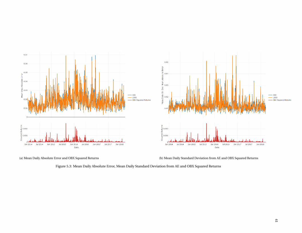
CH

AP

TE

R5.

RE

SULT

S41

(a) Mean Daily Absolute Error and OBX Squared Returns (b) Mean Daily Standard Deviation from AE and OBX Squared Returns

Figure 5.3: Mean Daily Absolute Error, Mean Daily Standard Deviation from AE and OBX Squared Returns


5.2.2 Return Generating Properties

In this subsection we will first evaluate the short-long strategy without transaction costs, and then evaluate the

same strategy with transaction costs. Finally, we will evaluate the bound strategy and discuss the choice of trading

bound.

Short-Long Strategy

As mentioned in Chapter 4, the short-long strategy is executed in order to assess the profitability of following the

out-of-sample, one-day-ahead return predictions of the forecasting model, and compare it to a common buy-and-

hold strategy. The short-long strategy will take a long position in a stock if the forecasting model predicts a positive

return, and a short position if the forecasting model predicts a negative return for the next day. The short-long

strategy’s return for a stock, a given day, is calculated as follows: if the model predicts the correct direction of the

out-of-sample, one-day-ahead realised return, the absolute value of the realised return is added to the current

accumulated return. Likewise, if the model predicts the wrong direction, the absolute value of the realised return

is subtracted from the current accumulated return.

Without Transaction Costs

The results from the short-long strategy without transaction costs are presented in Table 5.5 and Table 5.6 for sam-

ple sizes 500 and 1000, respectively. We observe from the average lines that the short-long strategy with both sam-

ple sizes outperform the buy-and-hold strategy, with a positive alpha. At the same time, the short-long strategy, for

both sample sizes, has the same volatility as the buy-and-hold strategy, generating a greater Sharpe ratio.

Further, the short-long strategy with sample size 1000 outperforms sample size 500 in terms of alpha, Sharpe

ratio and hit ratio. Firstly, the short-long strategy with sample size 1000 generates an annualised alpha of 3.51%

over four years, while the short-long strategy with sample size 500 generates an annualised alpha of 0.79% over the

same period. Secondly, the Sharpe ratio is also significantly better for the short-long strategy with sample size 1000

than the short-long strategy with sample size 500. Lastly, the hit ratio is marginally better for the short-long strategy

with sample size 1000 than the short-long strategy with sample size 500. The marginal increase in hit ratio appears

to account for the greater alpha and Sharpe ratio.

Furthermore, we observe that both sample sizes have a hit ratio close to, but below 50%. Assuming all market

shocks have equal magnitude, a hit ratio below 50% would generate a negative alpha. However, because market

shocks do not have equal magnitudes, it is possible to generate positive alphas with a hit ratio below 50%. As a

result, one can assert that the forecasting model can forecast the more substantial market shocks better.

The number of trades is less relevant evaluating a strategy when there are no transaction costs. However, when

introducing transaction costs into the trading environment, accounting for the number of trades made by the trad-

ing model becomes crucial. Notably, in a high-frequency trading model, such as ours, possibly executing daily

trades for all stocks, the number of trades is a key metric. The next subsection deals with this topic.

CH

AP

TE

R5.

RE

SULT

S43

Stock µB H σB H rB H Hit Ratio µSL σSL rSL α Total Trades SRB H SRSL

1 DNB 0.0003 0.0149 0.0812 0.4319 -0.0000 0.0149 -0.0028 -0.0840 859 0.3451 -0.0117

2 DNO -0.0005 0.0336 -0.1220 0.5093 -0.0008 0.0336 -0.2112 -0.0891 991 -0.2299 -0.3979

3 Norwegian -0.0001 0.0274 -0.0286 0.4981 0.0000 0.0274 0.0105 0.0390 1033 -0.0658 0.0241

4 Norsk Hydro 0.0005 0.0183 0.1339 0.4953 -0.0002 0.0183 -0.0566 -0.1904 969 0.4622 -0.1952

5 Petroleum Geo-Services -0.0009 0.0377 -0.2274 0.5056 0.0011 0.0377 0.2634 0.4908 899 -0.3814 0.4419

6 Questerre Energy Corporation 0.0000 0.0482 0.0065 0.4767 -0.0015 0.0482 -0.3717 -0.3782 887 0.0086 -0.4878

7 Statoil 0.0002 0.0172 0.0513 0.4841 0.0006 0.0172 0.1516 0.1003 847 0.1887 0.5577

8 Subsea 7 0.0000 0.0246 0.0009 0.4888 0.0005 0.0246 0.1332 0.1322 925 0.0024 0.3420

9 Telenor 0.0002 0.0139 0.0457 0.4562 -0.0005 0.0139 -0.1289 -0.1746 935 0.2073 -0.5856

10 Yara International 0.0002 0.0162 0.0609 0.5326 0.0012 0.0162 0.2941 0.2332 1089 0.2376 1.1503

Average 0.0000 0.0252 0.0002 0.4879 0.0000 0.0252 0.0082 0.0079 943 0.0775 0.0838

Table 5.5: Stock Metrics Without Transactions Costs For the Short-Long Trading Strategy and Sample Size 500


1 DNB 0.0003 0.0149 0.0812 0.4506 0.0005 0.0149 0.1152 0.0339 407 0.3451 0.4893

2 DNO -0.0005 0.0336 -0.1220 0.5037 0.0004 0.0336 0.0972 0.2192 1019 -0.2299 0.1831

3 Norwegian -0.0001 0.0274 -0.0286 0.4963 -0.0008 0.0274 -0.2028 -0.1742 1131 -0.0658 -0.4675

4 Norsk Hydro 0.0005 0.0183 0.1339 0.4804 0.0000 0.0183 0.0080 -0.1259 885 0.4622 0.0275

5 Petroleum Geo-Services -0.0009 0.0377 -0.2274 0.4944 -0.0010 0.0377 -0.2576 -0.0302 907 -0.3814 -0.4322

6 Questerre Energy Corporation 0.0000 0.0482 0.0065 0.5224 0.0010 0.0482 0.2610 0.2545 729 0.0086 0.3425

7 Statoil 0.0002 0.0172 0.0513 0.4860 0.0004 0.0172 0.1052 0.0538 991 0.1887 0.3868

8 Subsea 7 0.0000 0.0246 0.0009 0.4757 -0.0003 0.0246 -0.0865 -0.0874 917 0.0024 -0.2222

9 Telenor 0.0002 0.0139 0.0457 0.4841 0.0007 0.0139 0.1769 0.1313 909 0.2073 0.8042

10 Yara International 0.0002 0.0162 0.0609 0.5196 0.0005 0.0162 0.1375 0.0766 1109 0.2376 0.5365

Average 0.0000 0.0252 0.0002 0.4913 0.0001 0.0252 0.0354 0.0351 900 0.0775 0.1648

Table 5.6: Stock Metrics Without Transactions Costs For the Short-Long Trading Strategy and Sample Size 1000


With Transactions Cost

The short-long strategy implies actively deciding on a new position in every stock, each day. In a worst-case sce-

nario, one has to change position from long to short, or the opposite, each day for all stocks. In other words, the

forecasting model could make two transactions each day for all stocks, buying and selling. From Table 3.2 in Chap-

ter 3, there are 1072 days in our rolling window, resulting in a worst-case scenario of 2144 trades being made.

We observe from Figure 5.7 and 5.8, that there are 943 and 900 trades executed for each stock on average, with

sample size 500 and 1000, respectively. We have assumed a transaction cost of 10 bps per trade, following the

average commission rates paid by institutional investors on global equity trades (41). This reduces the short-long

return on average by 94.30 and 90.00 percentage points over four years, respectively. Hence, the forecasting model

now generates negative annualised alphas on average, -21.21% and -17.48% with the sample size 500 and 100,

respectively. This provides clear evidence that the transaction costs of the trading, destroys the return generating

abilities of the forecasting model when employing the short-long strategy. For reference, our study shows that a

transaction cost of 0.5 bps and 1.5 bps for sample size 500 and 1000, respectively, would generate an annualised

alpha of 0.00%.

Notably, the number of trades made by the forecasting model with sample size 500 is more than with sample

size 1000. This shows that an increase in sample size gives more persistence in the forecasts, resulting in fewer

trades. These characteristics are in line the findings of Hwang et al. (40), who indicates that GARCH parameters

tend to be downward biased for larger sample sizes. The findings have significant implications for the choice of

sample size. Thus, to decrease the number of trades, a larger sample size appears to be a good choice.

Further, there are some interesting observations when looking at the results of the individual stocks. When

the sample size is 500, all the stocks, except Petroleum Geo-Services (PGS), contribute with negative alphas. The

annualised alphas range from -58.51% to 28.11% percentage points. These variations are undoubtedly not a prefer-

able scenario. However, when the sample size is 1000, we observe smaller variations across the stocks’ alphas. The

annualised alphas now range from -43.80% to 8.45% percentage points. Moreover, PGS now has a negative alpha,

while Questerre Energy Corporation (QEC) is the only stock having a positive alpha. As discussed above, this may

be caused by the persistence in the forecasts. Please see "Appendix C: Trading Strategies" for the short-long return

and alpha plots of all the stocks.

As the number of trades affects the return generating properties of the dynamic forecasting model, we aim to

reduce the number of trades, by introducing the bound strategy. The next subsection deals with this strategy and

its results.

CH

AP

TE

R5.

RE

SULT

S45


1 DNB 0.0003 0.0149 0.0812 0.4319 -0.0008 0.0149 -0.2031 -0.2843 859 0.3451 -0.8595

2 DNO -0.0005 0.0336 -0.1220 0.5093 -0.0018 0.0336 -0.4423 -0.3203 991 -0.2299 -0.8324

3 Norwegian -0.0001 0.0274 -0.0286 0.4981 -0.0009 0.0275 -0.2304 -0.2019 1033 -0.0658 -0.5299

4 Norsk Hydro 0.0005 0.0183 0.1339 0.4953 -0.0011 0.0183 -0.2825 -0.4164 969 0.4622 -0.9754

5 Petroleum Geo-Services -0.0009 0.0377 -0.2274 0.5056 0.0002 0.0377 0.0537 0.2811 899 -0.3814 0.0902


7 Statoil 0.0002 0.0172 0.0513 0.4841 -0.0002 0.0172 -0.0459 -0.0973 847 0.1887 -0.1684

8 Subsea 7 0.0000 0.0246 0.0009 0.4888 -0.0003 0.0247 -0.0826 -0.0835 925 0.0024 -0.2117

9 Telenor 0.0002 0.0139 0.0457 0.4562 -0.0014 0.0139 -0.3470 -0.3926 935 0.2073 -1.5732

10 Yara International 0.0002 0.0162 0.0609 0.5326 0.0002 0.0162 0.0402 -0.0207 1089 0.2376 0.1572

Average 0.0000 0.0252 0.0002 0.4879 -0.0008 0.0252 -0.2118 -0.2121 943 0.0775 -0.5663

Table 5.7: Stock Metrics With Transaction Costs For the Short-Long Trading Strategy and Sample Size 500


1 DNB 0.0003 0.0149 0.0812 0.4506 0.0001 0.0149 0.0203 -0.0610 407 0.3451 0.0858

2 DNO -0.0005 0.0336 -0.1220 0.5037 -0.0006 0.0336 -0.1405 -0.0184 1019 -0.2299 -0.2642

3 Norwegian -0.0001 0.0274 -0.0286 0.4963 -0.0019 0.0275 -0.4666 -0.4380 1131 -0.0658 -1.0740

4 Norsk Hydro 0.0005 0.0183 0.1339 0.4804 -0.0008 0.0184 -0.1984 -0.3323 885 0.4622 -0.6835

5 Petroleum Geo-Services -0.0009 0.0377 -0.2274 0.4944 -0.0019 0.0377 -0.4691 -0.2417 907 -0.3814 -0.7870


7 Statoil 0.0002 0.0172 0.0513 0.4860 -0.0005 0.0172 -0.1260 -0.1773 991 0.1887 -0.4621

8 Subsea 7 0.0000 0.0246 0.0009 0.4757 -0.0012 0.0246 -0.3004 -0.3013 917 0.0024 -0.7708

9 Telenor 0.0002 0.0139 0.0457 0.4841 -0.0001 0.0139 -0.0351 -0.0807 909 0.2073 -0.1593

10 Yara International 0.0002 0.0162 0.0609 0.5196 -0.0005 0.0162 -0.1212 -0.1821 1109 0.2376 -0.4729

Average 0.0000 0.0252 0.0002 0.4913 -0.0007 0.0252 -0.1746 -0.1748 900 0.0775 -0.4469

Table 5.8: Stock Metrics With Transaction Costs For the Short-Long Trading Strategy and Sample Size 1000


Bound Strategy

As the short-long strategy with transaction costs destroys the return generating properties of the return forecasting

model, we will try a new trading strategy, the bound strategy, to reduce the number of trades. The bound strategy

aims to discard forecasting noise and only trade when the return forecasting model signals larger market shocks,

thus reducing the number of trades. As mentioned in Chapter 4, Methodology, we measure the trading bound, the

threshold for taking a position, as the percentage of the ARMA-GARCH’s out-of-sample, one-day-ahead volatility

forecast, obtained from the currently fitted ARMA-GARCH forecasting model.

The trading bounds for the respective sample sizes was found by plotting the average alpha against the trading

bound. In addition, to gain an overall understanding of the impact of the trading bound level, we plot the number of

transactions against the trading bound and the average hit ratio against the trading bound. These plots are showed

in Figure 5.4 and Figure 5.5, with sample size 500 and sample size 1000, respectively. We observe from Figure 5.4a

and Figure 5.5a that it is possible to choose trading bounds that would generate a positive alpha. However, we do

not choose these bounds, as the number of trades is close to zero, as observed in Figure 5.4b and Figure 5.5b. The

trading bounds chosen are trade-offs between alphas generated and the number of transactions. We believe that a

trading strategy that does, for example, ten trades over a period of four years, is not comparable to the short-long

strategy which does several hundred trades over the same period. Note that when the trading bound is zero, the

bound strategy is equivalent to the short-long strategy.

In Table 5.9 and 5.10 we show the bound strategy results with sample size 500 and 1000 and their chosen trading

bounds of 50% and 35%, respectively. From the bound strategy results, we observe that the hit ratios have increased

and the number of trades has significantly decreased compared to the short-long strategy, just as desired. The

alphas and Sharpe ratios are also improved compared to the short-long strategy. In addition, the risk has been

greatly reduced. Although the bound strategy outperforms the short-long strategy, it falls short of the buy-and-hold

strategy, on average. The bound strategy has negative returns, alphas and Sharpe ratios, whereas the buy-and-hold

has positive return and Sharpe ratio. The transaction costs are, still, too return destroying.

Comparing the bound strategy with sample size 500 and sample size 1000, we observe that the latter has the

better hit ratio and alpha, while the former has a slightly better Sharpe ratio. In addition, the bound strategy with

sample size 500 does more trades than the same strategy with sample size 1000. This result signifies the downward

bias of larger sample sizes. Overall, the short-long and bound strategy considered, the forecasting model appears

to perform best when trading according to the bound strategy with sample size 1000 and trading bound 35%.

An interesting observation is the performance of the forecasting model for high-volatility stocks. It generates

significant positive alphas for four of the five high-volatility stocks in this analysis, for both sample sizes. As we

have only included ten stocks in this sample, the characterisation of the stocks the forecasting model predicts the

best is hard to conclude. However, there is a trend that there exist return patterns in high-volatility stocks that the

ARMA-GARCH forecasting model, combined with the bound strategy, manages to capture. This is consistent with

the findings of Kim et al. (18). Please see "Appendix C: Trading Strategies" for the bound return and alpha plots of

all the individual stocks.

CH

AP

TE

R5.

RE

SULT

S47

(a) Average Alpha (b) Average Number of Transactions (c) Average Hit Ratio

Figure 5.4: Trading Bound: Sample Size 500

(a) Average Alpha (b) Average Number of Transactions (c) Average Hit Ratio

Figure 5.5: Trading Bound: Sample Size 1000

CH

AP

TE

R5.

RE

SULT

S48

Stock µB H σB H rB H Hit Ratio µB ound σB ound rB ound α Total Trades SRB H SRB ound

1 DNB 0.0003 0.0149 0.0812 0.7589 -0.0002 0.0062 -0.0476 -0.1288 90 0.3451 -0.4831

2 DNO -0.0005 0.0336 -0.1220 0.5843 0.0001 0.0097 0.0293 0.1514 117 -0.2299 0.1919

3 Norwegian -0.0001 0.0274 -0.0286 0.5682 0.0001 0.0080 0.0150 0.0436 98 -0.0658 0.1187

4 Norsk Hydro 0.0005 0.0183 0.1339 0.6031 0.0001 0.0058 0.0258 -0.1080 101 0.4622 0.2824

5 Petroleum Geo-Services -0.0009 0.0377 -0.2274 0.4571 -0.0005 0.0127 -0.1305 0.0968 100 -0.3814 -0.6487


7 Statoil 0.0002 0.0172 0.0513 0.6124 0.0001 0.0078 0.0215 -0.0298 183 0.1887 0.1740

8 Subsea 7 0.0000 0.0246 0.0009 0.6949 0.0005 0.0093 0.1259 0.1250 124 0.0024 0.8574

9 Telenor 0.0002 0.0139 0.0457 0.6392 -0.0001 0.0047 -0.0293 -0.0750 84 0.2073 -0.3965


Average 0.0000 0.0252 0.0002 0.6205 -0.0001 0.0097 -0.0233 -0.0236 114 0.0775 -0.0393

Table 5.9: Stock Metrics With Transaction Costs For the Bound Strategy With Trading Bound 0.5 and Sample Size 500

Stock µB H σB H rB H Hit Ratio µB ound σB ound rB ound α Total Trades SRB H SRB ound

1 DNB 0.0003 0.0149 0.0812 1.0000 0.0000 0.0000 0.0000 -0.0812 0 0.3451 0.0000

2 DNO -0.0005 0.0336 -0.1220 0.6211 0.0002 0.0091 0.0522 0.1742 81 -0.2299 0.3636

3 Norwegian -0.0001 0.0274 -0.0286 0.6104 0.0001 0.0056 0.0236 0.0521 76 -0.0658 0.2649

4 Norsk Hydro 0.0005 0.0183 0.1339 0.6226 -0.0000 0.0057 -0.0037 -0.1376 79 0.4622 -0.0410

5 Petroleum Geo-Services -0.0009 0.0377 -0.2274 0.5280 -0.0004 0.0134 -0.1109 0.1165 94 -0.3814 -0.5233


7 Statoil 0.0002 0.0172 0.0513 0.5972 -0.0004 0.0073 -0.1021 -0.1535 147 0.1887 -0.8841

8 Subsea 7 0.0000 0.0246 0.0009 0.6474 -0.0003 0.0087 -0.0771 -0.0780 99 0.0024 -0.5621

9 Telenor 0.0002 0.0139 0.0457 0.6667 -0.0003 0.0045 -0.0676 -0.1133 50 0.2073 -0.9512


Average 0.0000 0.0252 0.0002 0.6787 0.0000 0.0078 -0.0015 -0.0018 81 0.0775 -0.0876

Table 5.10: Stock Metrics With Transaction Costs For the Bound Strategy With Trading Bound 0.35 and Sample Size 1000

6. Conclusions

We have performed an extensive evaluation of a dynamic ARMA-GARCH forecasting model. Firstly, we highlighted

the dynamic forecasting model behaviour, by investigating the values of the forecasting model’s input parameters

- the GARCH model, AR-lag, MA-lag and the underlying return distribution - over time. Secondly, we described

the dynamic forecasting model in detail and then evaluated it in terms of both statistical and return generating

properties, without transaction costs. Thirdly, we described how the dynamic forecasting model could be used for

trading purposes in real-life scenarios, by considering two trading strategies and transaction costs.

6.1 Dynamic Forecasting Model Behaviour

The behaviour of the input parameters of the dynamic ARMA-GARCH forecasting model had some clear character-

istics. The E-GARCH-M was the dominant model, with an average fit of 51% and 64% with the sample size 500 and

1000, respectively. Also, the GJR-GARCH-M appears to be a good fit for the stocks, with an average fit of 37% and

29% with the sample size 500 and 1000, respectively. The S-GARCH is lagging the other two, with significantly less

fit over the rolling window, for both sample sizes. The leverage effect is present in stock returns, and thus a model,

such as E-GARCH-M or GJR-GARCH-M, is appropriate to capture the return movements. This is consistent with

the findings of Erdem et al. (31). Also, this effect is even more evident when the sample size increases from 500 to

1000.

The impact from the inclusion of the conditional volatility in the conditional mean equation is also interesting.

As both the E-GARCH-M and GJR-GARCH-M outperforms the S-GARCH in terms of fit, one could assert that the

in-mean modification is important for stock return modelling. This is also argued by Hansson and Hördahl (27)

and Liu et al. (30). However, as there was no E-GARCH or GJR-GARCH, without the in-mean term, in this analysis,

the marginal impact of the volatility feedback inclusion is hard to determine.

The AR and MA lag are somewhat constant over time, with an average of 4.15 and 3.84 with sample size 500,

respectively. With sample size 1000, these numbers are 3.72 and 3.51. Moreover, both the AR-lag and MA-lag seem

somewhat unaffected by current market conditions. This is interesting given the findings in Section 3.2, showing

the ACF and PACF results from lag 1 to 12, for all the stocks. Here, results indicated that one should not find any

specific pattern in the autocorrelations for the different lags, across the whole rolling window. However, we observe

that a fitted ARMA-GARCH model often chooses to include several AR-lags. An explanation may be variations in

49

CHAPTER 6. CONCLUSIONS 50

the autocorrelation across sample windows, although there are few lags which are significant over the whole rolling

window.

Moreover, we find that the generalised error distribution (GED) is the most common best fit. Half of the stocks

considered fit this distribution the best. This finding matches what was also indicated by Gysen et al. (42), who

argued that leptokurtic innovations for the E-GARCH-M are very consistent. Further, none of the stocks matches

the normal distribution overall best, emphasising that the assumption of normally distributed returns is usually

not valid. Notably, the generalised hyperbolic function distribution, the student t distribution, the skewed student

t distribution and the normal inverse Gaussian distribution are also among the best-fitted distributions.

6.2 The Performance of the Forecasting Model Without Transaction Costs

Considering the statistical metrics of the forecasting model, we observe a significant, positive relationship between

the mean daily absolute error, mean daily standard deviation from the absolute error and the market volatility. The

positive relationship implies that high volatility in the market tends to increase the average forecasting error.

Further, there appear to be small differences between the two sample sizes, both for the stocks’ mean daily

absolute error and the mean daily standard deviation from absolute error, regardless of the market volatility. Also,

large values of MAE and standard deviation from AE do not necessarily result in decreased trading returns, as the

forecast of the return direction is what influences the trading decision.

The results show that the short-long strategy with no transaction costs outperforms the buy-and-hold strategy,

with a positive alpha and greater Sharpe ratio, for both sample sizes. Moreover, the short-long strategy with sample

size 1000 outperforms sample size 500 in terms of alpha, Sharpe ratio and hit ratio. The short-long strategy with

sample size 1000 generates an annualised alpha of 3.51%, while the short-long strategy with sample size 500 gen-

erates an annualised alpha of 0.79%. Lastly, we observe that both sample sizes have a hit ratio close to, but below

50%. As market shocks have different magnitude, the strategy still manage to generate a positive alpha.

6.3 The Performance of the Forecasting Model With Transaction Costs

To assess the forecasting model in a real-life scenario, we included transaction costs. The forecasting model, ex-

ecuting the short-long strategy, now generates negative alphas on average, namely -21.21% and -17.48% with the

sample size 500 and 1000, respectively.

Further, the performance of the forecasting model with sample size 1000 is better than with sample size 500.

An increase in sample size gives more persistence in the forecasts, resulting in fewer trades. These characteristics

are consistent with the findings of Hwang et al. (40), who indicates that GARCH parameters tend to be downward

biased for larger sample sizes. The findings have significant implications for the choice of sample size. Thus,

to decrease the number of trades, a larger sample size appears to be a good choice. However, regardless of the

chosen sample size, the results provide clear evidence that the transaction costs of the trading, destroys the return

generating abilities of the forecasting model when executing the short-long strategy.

CHAPTER 6. CONCLUSIONS 51

As a result, to reduce the number of trades, we introduced the bound strategy. The results from this strategy

show that the hit ratios have increased and the number of trades significantly decreased, compared to the short-

long strategy, just as desired. Although the bound strategy outperforms the short-long strategy, it falls short of the

buy-and-hold strategy, on average. The bound strategy has negative returns, alphas and Sharpe ratios, whereas the

buy-and-hold has positive return and Sharpe ratio. The transaction costs are, still, too return destroying.

Comparing the bound strategy with sample size 500 and sample size 1000, we observe that the latter has the

better hit ratio and alpha, while the former has a slightly better Sharpe ratio. In addition, the bound strategy with

sample size 500 does more trades than the same strategy with sample size 1000. This result signifies the downward

bias of larger sample sizes. Overall, the short-long and bound strategy considered, the forecasting model appears

to perform best when trading according to the bound strategy with sample size 1000 and trading bound 35%.

Hence, the performance of the forecasting model indicate that the market is efficient. Without transaction

costs, there are statistical patterns in return series that in theory can be exploited to generate a positive alpha.

However, as our study is extended to include transaction costs, we show that the return forecasting performance

is destroyed, which has important implications. The transaction costs make the market efficient. Investors and

traders can not profitably make use of the statistical information in the return series.

However, an interesting observation is the forecasting model’s performance on high-volatility stocks. The fore-

casting model generates significant positive alphas for four of the five high-volatility stocks in this analysis, for

both sample sizes with the bound strategy. This is aligned with the findings of Kim et al. (18). As we have only

included ten stocks in this sample, the overall characterisation of the stocks which the forecasting model predicts

the best is hard to conclude. However, there is a trend that there exist return patterns in high-volatility stocks that

the ARMA-GARCH forecasting model, combined with the bound strategy, manages to capture.

6.4 Concluding Remarks

We have shown that a dynamic ARMA-GARCH forecasting model can work, especially when considering the bound

strategy with sample size 1000 and trading bound 35%. Also, the model seems to predict the returns of high-

volatility stocks very well. A large sample size, few trades and high-volatility stocks appears to be key characteristics

for generating a positive alpha using a dynamic ARMA-GARCH to forecast returns.

On reflection, the computational complexity is an issue. Our results assert the dominance of E-GARCH-M, the

tendency of constant ARMA(4,4), and a generalised error distribution (GED) to be the best fit for stocks. One could

thus argue that a fixed ARMA(4,4)-E-GARCH(1,1)-M, with GED as the underlying distribution, would be a good

choice for a fixed forecasting model. This will generate a forecasting model with the need of only one model fit

for each day in the rolling window, for each stock. Thus, the computational complexity would be reduced to a

minimum. On the other hand, it is difficult to assess whether the daily model fitting is what makes the model work,

despite the seemingly mean-reverting behaviour.

7. Future Work

We have devoted a chapter to future work, as we have many ideas on how improve the forecasting performance of

the ARMA-GARCH.

The initial results indicate that the model performs well on high-volatility stocks. To address and verify this find-

ing, we must test the forecasting model on more stocks, especially high-volatile, both in Norway and globally. The

finding can also be substantiated through sub-period analysis, looking at the performance of the trading strategies

during high-volatile periods. If the hypothesis is correct, running the forecasting model on other types of financial

assets, such as high-volatile commodities or cryptocurrencies, is tempting.

Testing the forecasting model performance over a longer rolling window is essential. Due to computational

complexity, we only tested the forecasting model on four years of data. To further verify the performance, testing

over more years is necessary, and will also enable us to check the model performance under even more kinds of

market conditions.

In reality, the cost of short selling is greater than the cost of buying, as one would need to pay a loan fee over

the shorting period. Consequently, it is reasonable to assume that transaction costs would destroy returns even

more than presented in this study, as both the short-long and the bound strategy use short selling. In addition,

some stocks might not be available for short selling. A possible solution would be to implement a modification of

the bound strategy that does not use short selling. Obviously, such a strategy would miss the potential upside of

correctly forecasting and leveraging market downturns.

The initial results signify that the forecasting model performs better with sample size 1000 than with 500. To

examine whether a larger sample size is a success criterion for the forecasting model, we need to test for even larger

sample sizes, such as 1500 or even 2000. This will increase the computational complexity, while possibly enhancing

the forecasting model performance.

Further, it would be interesting to modify the ARMA-GARCH model even more. The E-GARCH-M was the best

fit for the stocks in this study, but testing for other GARCH models could prove successful. Models such as the Q-

GARCH-M or T-GARCH-M have properties not entirely captured by the E-GARCH-M or GJR-GARCH-M. Modifying

the conditional mean equation to an ARMAX model, by also including other lagged explanatory variables, such as

the oil price, is another possible extension.

Lastly, a next step would be to test the forecasting model’s performance on intraday data. There is possibly more

autocorrelation in returns in shorter time spans, and hence better conditions for the forecasting model. Another

52

CHAPTER 7. FUTURE WORK 53

important implication of running on intraday data would be the possibility to optimise the holding time for each

stock, given the previous day’s forecasting prediction. As we forecast the one-day-ahead return, realising positions

during intraday movements could enhance returns.

Collectively, we believe there are several promising extensions to the forecasting model, to enhance returns and

make the forecasting model even more applicable in real-life scenarios.

Bibliography

[1] PWC (2017), Global Assets under Management set to rise to $145.4 trillion by 2025, From:

https://press.pwc.com/News-releases/global-assets-under-management-set-to-rise-to–145.4-trillion-by-

2025/s/e236a113-5115-4421-9c75-77191733f15f

[2] Harry Markowitz, Portfolio Selection, The Journal of Finance, Vol. 7, No.1., 1952

[3] James E. McWhinney, Investopedia (2018), Quantitative analysis: A simple overview, From:

https://www.investopedia.com/articles/investing/041114/simple-overview-quantitative-analysis.asp

[4] Merton, R. C. (1973). Theory of rational option pricing. The Bell Journal of economics and management science,

141-183.

[5] Robin Wigglesworth, Financial Times (2018), Quant hedge funds set to surpass $1tn management mark, From:

https://www.ft.com/content/ff7528bc-ec16-11e7-8713-513b1d7ca85a

[6] Mandelbrot, B. (1963). New methods in statistical economics. Journal of political economy, 71(5), 421-440.

[7] T. Bollerslev, Generalized autoregressive conditional heteroscedasticity, J. Econ. 31 (1986), pp. 307–327.

[8] R.F. Engle, Autoregressive conditional heteroscedasticity with estimates of the variance of United Kingdom infla-

tion, Econometrica 50 (1982), pp. 987–1007.

[9] Robert Engle, Stern School of Business, New York University, An Introduction to the Use of ARCH/GARCH models

in Applied Econometrics, From: http://www.stern.nyu.edu/rengle/GARCH101.PDF

[10] Shiller, R. J. (2003). From efficient markets theory to behavioral finance. Journal of economic perspectives,

17(1), 83-104.

[11] Merton, R. C. (1973). An intertemporal capital asset pricing model. Econometrica: Journal of the Econometric

Society, 867-887.

[12] Lucas Jr, R. E. (1978). Asset prices in an exchange economy. Econometrica: Journal of the Econometric Society,

1429-1445.

[13] Shiller, R. J. (1981). The use of volatility measures in assessing market efficiency. The Journal of Finance, 36(2),

291-304.

54

BIBLIOGRAPHY 55

[14] Fama, E. F., French, K. R. (1996). Multifactor explanations of asset pricing anomalies. The journal of finance,

51(1), 55-84.

[15] Barberis, N., Shleifer, A., Vishny, R. (1998). A model of investor sentiment1. Journal of financial economics,

49(3), 307-343.

[16] Fama, E. F. (1991). Efficient capital markets: II. The journal of finance, 46(5), 1575-1617.

[17] F. Fu, Idiosyncratic risk and the cross-section of expected stock returns, Journal of Financial Economics, Volume

91, Issue 1, 2009, pp. 24-37.

[18] Kim, J. H., Shamsuddin, A., Lim, K. P. (2011). Stock return predictability and the adaptive markets hypothesis:

Evidence from century-long US data. Journal of Empirical Finance, 18(5), 868-879.

[19] Skjeltorp, J. A. (2000). Scaling in the Norwegian stock market. Physica A: Statistical Mechanics and its Applica-

tions, 283(3-4), 486-528.

[20] Næs, R., Skjeltorp, J. A., Ødegaard, B. A. (2011). Stock market liquidity and the business cycle. The Journal of

Finance, 66(1), 139-176.

[21] Nygaard, K. (2011). The disposition effect and momentum: Evidence from norwegian household investors.

[22] Weron, R., Misiorek, A. (2005, May). Forecasting spot electricity prices with time series models. In Proceedings

of the European Electricity Market EEM-05 Conference (pp. 133-141).

[23] Campbell, J. Y., Lo, A. W. C., MacKinlay, A. C. (1997). The econometrics of financial markets (Vol. 2, pp. 149-

180). Princeton, NJ: princeton University press.

[24] Nelson, D. B. (1991). Conditional heteroskedasticity in asset returns: A new approach. Econometrica: Journal

of the Econometric Society, 347-370.

[25] Engle, R. F., Ng, V. K., Rothschild, M. (1990). Asset pricing with a factor-ARCH covariance structure: Empirical

estimates for treasury bills. Journal of Econometrics, 45(1-2), 213-237.

[26] Glosten, L. R., Jagannathan, R., Runkle, D. E. (1993). On the relation between the expected value and the

volatility of the nominal excess return on stocks. The journal of finance, 48(5), 1779-1801.

[27] Hansson, B., Hördahl, P. (1997). Changing risk premia: evidence from a small open economy. The Scandina-

vian Journal of Economics, 99(2), 335-350.

[28] Glosten, L. R., Jagannathan, R., Runkle, D. E. (1993). On the relation between the expected value and the

volatility of the nominal excess return on stocks. The journal of finance, 48(5), 1779-1801.

[29] Engle, R. F., Lilien, D. M., Robins, R. P. (1987). Estimating time varying risk premia in the term structure: The

ARCH-M model. Econometrica: Journal of the Econometric Society, 391-407.

BIBLIOGRAPHY 56

[30] Liu, H., Erdem, E., Shi, J. (2011). Comprehensive evaluation of ARMA–GARCH (-M) approaches for modeling

the mean and volatility of wind speed. Applied Energy, 88(3), 724-732.

[31] Liu, H., Erdem, E., Shi, J. (2011). Comprehensive evaluation of ARMA–GARCH (-M) approaches for modeling

the mean and volatility of wind speed. Applied Energy, 88(3), 724-732.

[32] Higgins, M. L., Bera, A. K. (1992). A class of nonlinear ARCH models. International Economic Review, 137-158.

[33] Sentana, E. (1995). Quadratic ARCH models. The Review of Economic Studies, 62(4), 639-661.

[34] Bowden, N., Payne, J. E. (2008). Short term forecasting of electricity prices for MISO hubs: Evidence from

ARIMA-EGARCH models. Energy Economics, 30(6), 3186-3197.

[35] McNeil, A. J., Frey, R. (2000). Estimation of tail-related risk measures for heteroscedastic financial time series:

an extreme value approach. Journal of empirical finance, 7(3-4), 271-300.

[36] Bollerslev, T. (1987). A conditionally heteroskedastic time series model for speculative prices and rates of re-

turn. The review of economics and statistics, 542-547.

[37] Hansen, B. E. (1994). Autoregressive conditional density estimation. International Economic Review, 705-730.

[38] Brooks, C. (2002). Introductory econometrics for finance. Cambridge: Cambridge University Press.

[39] Zumbach, G. (2000). The pitfalls in fitting GARCH (1, 1) processes. In Advances in Quantitative Asset Manage-

ment (pp. 179-200). Springer, Boston, MA.

[40] Hwang, S., Valls Pereira, P. L. (2006). Small sample properties of GARCH estimates and persistence. The Euro-

pean Journal of Finance, 12(6-7), 473-494.

[41] Greenwich Associates (2015), Institutional Equity Trade Commission Rates Hold Steady Amid Volatility

and Market Structure Reform, From: https://www.greenwich.com/press-release/institutional-equity-trade-

commission-rates-hold-steady-amid-volatility-and-market

[42] van Gysen, M., Huang, C. S., Kruger, R. (2013). The performance of linear versus non-linear models in fore-

casting returns on the Johannesburg Stock Exchange. The International Business Economics Research Journal

(Online), 12(8), 985.

[43] Matías, J. M., Reboredo, J. C. (2012). Forecasting performance of nonlinear models for intraday stock returns.

Journal of Forecasting, 31(2), 172-188.

[44] Oslo Stock Exchange (2018), OBX Total Return Index, From: https://www.oslobors.no/ob_eng/markedsaktivitet//details/OBX.OSE/overview

[45] Netfonds (2018), Components for OBX Total Return Index, From: http://www.netfonds.no/quotes/peers.php?paper=OBXexchange=OSE

[46] G.E.P. Box and G.M. Jenkins, Time Series Analysis Forecasting and Control, Holden-Day, San Francisco, 1976.

BIBLIOGRAPHY 57

[47] Alexander, C. (2001). Market models: Practical Financial Econometrics. John Wiley Sons.

[48] J.B. Maverick, Investopedia (2018), What is a good Sharpe ratio?, From:

https://www.investopedia.com/ask/answers/010815/what-good-sharpe-ratio.aspixzz5ER0i3b9R

Appendices

58

Appendix A: Stocks Returns and Squared Returns

(a) Return Plot (b) Squared Return Plot

Figure 1: DNB


Figure 2: DNO

59

60


Figure 4: Norwegian Air Shuttle


Figure 3: Norsk Hydro

61


Figure 5: Petroleum Geo-Services


Figure 6: Questerre Energy Corporation

62


Figure 7: Statoil


Figure 8: Subsea 7

63


Figure 9: Telenor


Figure 10: Yara International

Appendix B: Stocks ACF and PACF

Returns

(a) Autocorrelation Function (b) Partial Autocorrelation Function

Figure 11: DNB

64

65


Figure 12: DNO



66





67




Figure 17: Statoil

68


Figure 18: Subsea 7


Figure 19: Telenor

69

(a) Autocorrelation Function (b) Squared Return Plot


Squared Returns


Figure 21: DNB

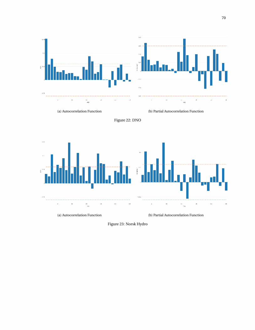
70


Figure 22: DNO



71





72




Figure 27: Statoil

73


Figure 28: Subsea 7


Figure 29: Telenor

74



Appendix C: Trading Strategies

Short-Long Strategy


Figure 31: DNB

75

76


Figure 32: DNO



77





78




Figure 37: Statoil

79


Figure 38: Subsea 7


Figure 39: Telenor

80



Bound Strategy


Figure 41: DNB

81


Figure 42: DNO



82





83




Figure 47: Statoil

84


Figure 48: Subsea 7


Figure 49: Telenor

85



a dynamic arma-garch model: forecasting returns and

Documents