1

Civil Systems PlanningBenefit/Cost Analysis

Scott Matthews12-706/19-702 / 73-359Lecture 7

12-706 and 73-359 2

Efficiency Definitions/Metrics

Allocative - resources are used at highest value possible

But welfare economics uses another:An allocation of goods is Pareto efficient if

no alternative allocation can make at least one person better off without making anyone else worse off. Inefficient if can re-allocate to make better

without making anyone else worse Assumed that decisions made with this in mind?

12-706 and 73-359 3

A Pareto Example

Try splitting $ between 2 people Get total ($100) if agree on how to split No agreement, each gets only $25

Pareto efficiency assumptions: More is better than less Resources are scarce Initial allocation matters

12-706 and 73-359 4

$100

$1000

Given this graph, how canWe describe the ‘set of all Possible splits between 2 peopleThat allocates the entire $100??

12-706 and 73-359 5

$100

$1000

Line is the ‘set of all possible splits that allocates the entire $100, Also called the potential pareto frontier. Is the line pareto efficient?

12-706 and 73-359 6

$100

$1000

No. Could at least get the ‘status quo’ result of (25,25) if they do not agree on splitting. So neither person would accept a split giving them less than $25. Is status quo pareto efficient?

$25

$25

12-706 and 73-359 7

$100

$1000

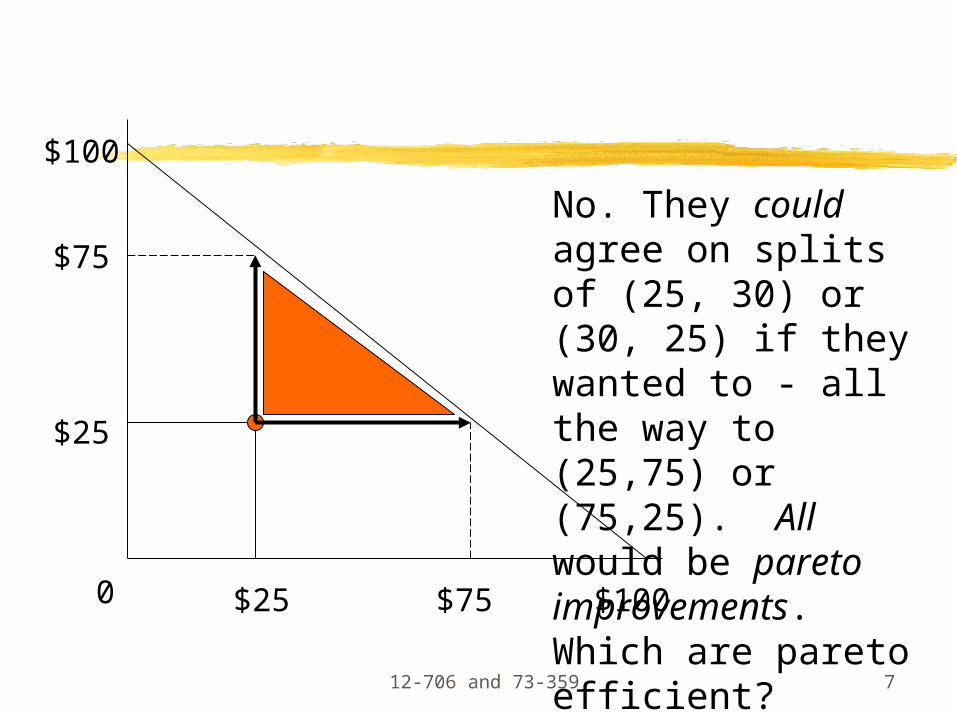
No. They could agree on splits of (25, 30) or (30, 25) if they wanted to - all the way to (25,75) or (75,25). All would be pareto improvements. Which are pareto efficient?

$25

$25

$75

$75

12-706 and 73-359 8

$100

$1000

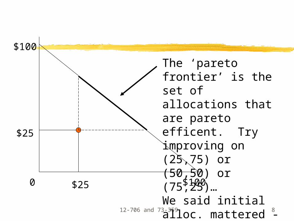
The ‘pareto frontier’ is the set of allocations that are pareto efficent. Try improving on (25,75) or (50,50) or (75,25)…We said initial alloc. mattered - e.g. (100,0)?

$25

$25

12-706 and 73-359 9

Pareto Efficiency and CBA

If a policy has NB > 0, then it is possible to transfer value to make some party better off without making another worse off.

To fully appreciate this, we need to understand willingness to pay and opportunity cost in light of CBA.

12-706 and 73-359 10

Willingness to Pay

Example: how much would everyone pay to build a mall ‘in middle of class’ Near middle may not want traffic costs Further away might enjoy benefits

Ask questions to find indifference pts.Relative to status quo (no mall)E.g. middle WTP -$2 M, edges +$3 MEdges could ‘pay off’ middle to buildOnly works if Net Benefits positive!

12-706 and 73-359 11

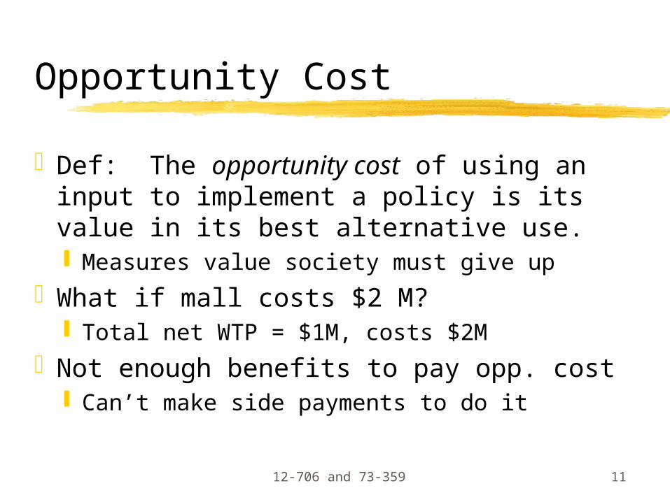
Opportunity Cost

Def: The opportunity cost of using an input to implement a policy is its value in its best alternative use. Measures value society must give up

What if mall costs $2 M? Total net WTP = $1M, costs $2M

Not enough benefits to pay opp. cost Can’t make side payments to do it

12-706 and 73-359 12

Wrap Up

As long as benefits found by WTP and costs by OC then sign of net benefits indicated whether side payments can make pareto improvements

Kaldor-Hicks criterion A policy should be adopted if and only if

gainers could fully compensate losers and still be better offPotential Pareto Efficiency (line on Fig 2.1)

12-706 and 73-359 13

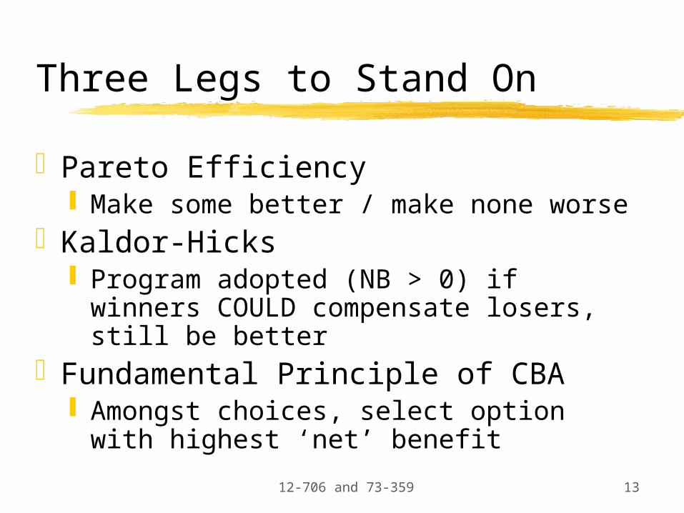
Three Legs to Stand On

Pareto Efficiency Make some better / make none worse

Kaldor-Hicks Program adopted (NB > 0) if winners

COULD compensate losers, still be better

Fundamental Principle of CBA Amongst choices, select option with

highest ‘net’ benefit

12-706 and 73-359 14

Welfare EconomicsConceptsPerfect Competition

Homogeneous goods. No agent affects prices. Perfect information. No transaction costs /entry issues No transportation costs. No externalities:

Private benefits = social benefits.Private costs = social costs.

12-706 and 73-359 15

Discussion - WTP

Survey of students of WTP for beer How much for 1 beer? 2 beers? Etc.

Does similar form hold for all goods? What types of goods different?

Economists also refer to this as demand

12-706 and 73-359 16

(Individual) Demand Curves Downward Sloping is a result of diminishing marginal

utility of each additional unit (also consider as WTP) Presumes that at some point you have enough to make

you happy and do not value additional units

Price

Quantity

P*

0 1 2 3 4 Q*

A

B

Actually an inverse demand curve (whereP = f(Q) instead).

12-706 and 73-359 17

Market DemandPrice

P*

0 1 2 3 4 Q

A

B

If above graphs show two (groups of) consumer demands, what is social demand curve?

P*

0 1 2 3 4 5 Q

A

B

12-706 and 73-359 18

Market Demand

Found by calculating the horizontal sum of individual demand curves

Market demand then measures ‘total consumer surplus of entire market’

P*

0 1 2 3 4 5 6 7 8 9 Q

12-706 and 73-359 19

Social WTP (i.e. market demand)

Price

Quantity

P*

0 1 2 3 4 Q*

A

B

‘Aggregate’ demand function: how all potential consumers in society value the good or service (i.e., someone willing to pay every price…)

This is the kind of demand curves we care about

12-706 and 73-359 20

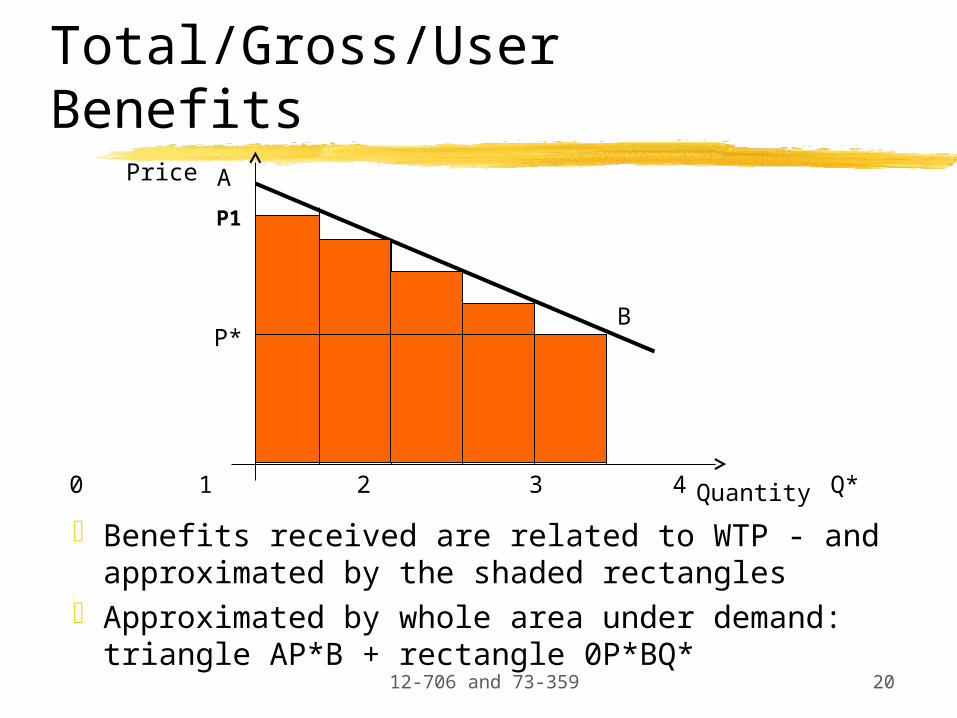
Total/Gross/User BenefitsPrice

Quantity

P*

0 1 2 3 4 Q*

A

B

Benefits received are related to WTP - and approximated by the shaded rectangles

Approximated by whole area under demand: triangle AP*B + rectangle 0P*BQ*

P1

12-706 and 73-359 21

Benefits with WTPPrice

Quantity

P*

0 1 2 3 4 Q*

A

B

Total/Gross/User Benefits = area under curve or willingness to pay for all people = Social WTP = their benefit from consuming = sum of all WTP values

Receive benefits from consuming this much regardless of how much they pay to get it

12-706 and 73-359 22

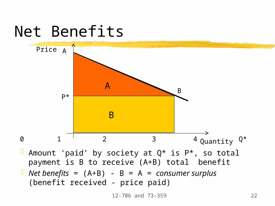
Net BenefitsPrice

Quantity

P*

0 1 2 3 4 Q*

A

BA

B

Amount ‘paid’ by society at Q* is P*, so total payment is B to receive (A+B) total benefit

Net benefits = (A+B) - B = A = consumer surplus (benefit received - price paid)

12-706 and 73-359 23

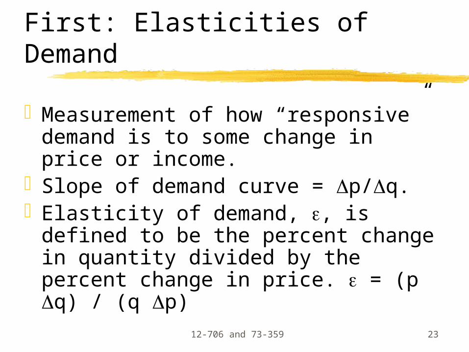
First: Elasticities of Demand

Measurement of how “responsive” demand is to some change in price or income.

Slope of demand curve = p/q.Elasticity of demand, , is defined to

be the percent change in quantity divided by the percent change in price. = (p q) / (q p)

12-706 and 73-359 24

Elasticities of DemandElastic demand: > 1. If P inc. by 1%, demand dec. by more than 1%.Unit elasticity: = 1. If P inc. by 1%, demand dec. by 1%.Inelastic demand: < 1 If P inc. by 1%, demand dec. by less than 1%.

Q

P

Q

P

12-706 and 73-359 25

Elasticities of Demand

Q

P

Q

P

PerfectlyInelastic

PerfectlyElastic

A change in price causesDemand to go to zero(no easy examples)

Necessities, demand isCompletely insensitiveTo price

12-706 and 73-359 26

Elasticity - Some Formulas

Point elasticity = dq/dp * (p/q)For linear curve, q = (p-a)/b so dq/dp

= 1/bLinear curve point elasticity =(1/b)

*p/q = (1/b)*(a+bq)/q =(a/bq) + 1

12-706 and 73-359 27

Maglev System Example

Maglev - downtown, tech center, UPMC, CMU

20,000 riders per day forecast by developers.

Let’s assume price elasticity -0.3; linear demand; 20,000 riders at average fare of $ 1.20. Estimate Total Willingness to Pay.

12-706 and 73-359 28

Example calculations

We have one point on demand curve: 1.2 = a + b*(20,000)

We know an elasticity value: elasticity for linear curve = 1 + a/bq -0.3 = 1 + a/b*(20,000)

Solve with two simultaneous equations: a = 5.2 b = -0.0002 or 2.0 x 10^-4

12-706 and 73-359 29

Demand Example (cont)

Maglev Demand Function: p = 5.2 - 0.0002*q

Revenue: 1.2*20,000 = $ 24,000 per day

TWtP = Revenue + Consumer Surplus TWtP = pq + (a-p)q/2 = 1.2*20,000 +

(5.2-1.2)*20,000/2 = 24,000 + 40,000 = $ 64,000 per day.

12-706 and 73-359 30

Change in Fare to $ 1.00 From demand curve: 1.0 = 5.2 - 0.0002q, so q

becomes 21,000. Using elasticity: 16.7% fare change (1.2-1/1.2), so q

would change by -0.3*16.7 = 5.001% to 21,002 (slightly different value)

Change to Revenue = 1*21,000 - 1.2*20,000 = 21,000 - 24,000 = -3,000.

Change CS = 0.5*(0.2)*(20,000+21,000)= 4,100 Change to TWtP = (21,000-20,000)*1 + (1.2-

1)*(21,000-20,000)/2 = 1,100.

12-706 and 73-359 31

Estimating Linear Demand Functions

As above, sometimes we don’t know demand Focus on demand (care more about CS) but can

use similar methods to estimate costs (supply) Ordinary least squares regression used

minimize the sum of squared deviations between estimated line and p,q observations: p = a + bq + e

Standard algorithms to compute parameter estimates - spreadsheets, Minitab, S, etc.

Estimates of uncertainty of estimates are obtained (based upon assumption of identically normally distributed error terms).

Can have multiple linear terms

12-706 and 73-359 32

Log-linear Function

q = a(p)b(hh)c….. Conditions: a positive, b negative, c positive,... If q = a(p)b : Elasticity interesting = (dq/dp)*(p/q)

= abp(b-1)*(p/q) = b*(apb/apb) = b. Constant elasticity at all points.

Easiest way to estimate: linearize and use ordinary least squares regression (see Chap 12) E.g., ln q = ln a + b ln(p) + c ln(hh) ..

12-706 and 73-359 33

Log-linear Function

q = a*pb and taking log of each side gives: ln q = ln a + b ln p which can be re-written as q’ = a’ + b p’, linear in the parameters and amenable to OLS regression.

This violates error term assumptions of OLS regression.

Alternative is maximum likelihood - select parameters to max. chance of seeing obs.

12-706 and 73-359 34

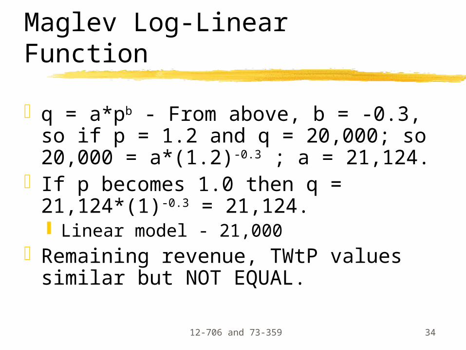
Maglev Log-Linear Function

q = a*pb - From above, b = -0.3, so if p = 1.2 and q = 20,000; so 20,000 = a*(1.2)-0.3 ; a = 21,124.

If p becomes 1.0 then q = 21,124*(1)-0.3 = 21,124. Linear model - 21,000

Remaining revenue, TWtP values similar but NOT EQUAL.

12-706 and 73-359 35

BCA Part 2: CostWelfare Economics Continued

The upper segment of a firm’s marginal cost curve correspondsto the firm’s SR supply curve. Again, diminishing returns occur.

Quantity

Price

Supply=MCAt any given price, determineshow much output to produce tomaximize profit

AVC

12-706 and 73-359 36

Supply/Marginal Cost Notes

Quantity

Price Supply=MCAt any given price, determineshow much output to produce tomaximize profit

P*

Q1 Q* Q2

Demand: WTP for each additional unitSupply: cost incurred for each additional unit

12-706 and 73-359 37

Supply/Marginal Cost Notes

Quantity

Price Supply=MCArea under MC is TVC - why?

P*

Q1 Q* Q2

Recall: We always want to be considering opportunity costs (total asset value to society) and not accounting costs

12-706 and 73-359 38

Monopoly - the real game

One producer of good w/o substituteNot example of perfect comp!

Deviation that results in DWL There tend to be barriers to entry Monopolist is a price setter not taker

Monopolist is only firm in market Thus it can set prices based on output

12-706 and 73-359 39

Monopoly - the real game (2)

Could have shown that in perf. comp. Profit maximized where p=MR=MC (why?)

Same is true for a monopolist -> she can make the most money where additional revenue = added cost But unlike perf comp, p not equal to MR

12-706 and 73-359 40

Monopoly Analysis

MR D

MC

Qc

Pc

In perfect competition,Equilibrium was at (Pc,Qc) - where S=D.

But a monopolist has aFunction of MR that Does not equal Demand

So where does he supply?

12-706 and 73-359 41

Monopoly Analysis (cont.)

MRD

MC

Qc

Pc

Monopolist supplies where MR=MC for quantity to max.profits (at Qm)

But at Qm, consumersare willing to pay Pm!

What is social surplus, Is it maximized?

Qm

Pm

12-706 and 73-359 42

Monopoly Analysis (cont.)

MRD

MC

Qc

Pc

What is social surplus?Orange = CS

Yellow = PS (bigger!)

Grey = DWL (from notProducing at Pc,Qc) thusSoc. Surplus is not maximized

Breaking monopolyWould transfer DWL toSocial Surplus

Qm

Pm

12-706 and 73-359 43

Natural Monopoly

Fixed costs very large relative to variable costs Ex: public utilities (gas, power, water)

Average costs high at low outputAC usually higher than MCOne firm can provide good or service

cheaper than 2+ firms In this case, government allows monopoly but

usually regulates it

12-706 and 73-359 44

Natural Monopoly

MRDQ*

P*

Faced with these curvesNormal monop wouldProduce at Qm and Charge Pm.

We would have sameSocial surplus.

But natural monopoliesAre regulated.

What are options?Qm

Pm

MC

AC

a

bc

d

e

12-706 and 73-359 45

Natural Monopoly

MR

D

Q*

P*

Forcing the price P*Means that the social surplus is increased.

DWL decreases from abc to dec

Society gains adeb

Qm

Pm

MC

AC

a

bc

d

e

Q0

12-706 and 73-359 46

Monopoly

Other options - set P = MC But then the firm loses money Subsidies needed to keep in business

Give away good for free (e.g. road) Free rider problems Also new deadweight loss from cost

exceeding WTP

12-706 and 73-359 47

Pricing Strategies

Highway pricing If price set equal to AC (which is assumed to be TC/q

then at q, total costs covered p ~ AVC: manages usage of highway p = f(fares, fees, travel times, discomfort) Price increase=> less users (BCA) MC pricing: more users, higher price What about social/external costs? Might want to set p=MSC