1. introduction. - tygert

SIAM J. SCI. COMPUT. c© 2006 Society for Industrial and Applied MathematicsVol. 27, No. 6, pp. 1903–1928

FAST ALGORITHMS FOR SPHERICAL HARMONIC EXPANSIONS∗

VLADIMIR ROKHLIN† AND MARK TYGERT‡

Abstract. An algorithm is introduced for the rapid evaluation at appropriately chosen nodeson the two-dimensional sphere S2 in R

3 of functions specified by their spherical harmonic expansions(known as the inverse spherical harmonic transform), and for the evaluation of the coefficients inspherical harmonic expansions of functions specified by their values at appropriately chosen pointson S2 (known as the forward spherical harmonic transform). The procedure is numerically stableand requires an amount of CPU time proportional to N2(logN) log(1/ε), where N2 is the numberof nodes in the discretization of S2, and ε is the precision of computations. The performance of thealgorithm is illustrated via several numerical examples.

Key words. spherical harmonics, fast algorithms, expansions

AMS subject classification. 65T50

DOI. 10.1137/050623073

1. Introduction. Spherical harmonic expansions are a widely used and well-understood tool of applied mathematics; they are encountered, inter alia, in weatherand climate modeling, in the representation of gravitational, topographic, and mag-netic data in geophysics, in the numerical solution of certain partial differential equa-tions, etc. The role of spherical harmonic expansions in diagonalizing the Laplacianin three dimensions is similar to the role played by Fourier series expansions in twodimensions.

The spherical harmonic expansion of a function f in L2(S2) is the series of theform

f(θ, ϕ) =

∞∑l=0

l∑m=−l

αml P

|m|l (cos θ) eimϕ,(1.1)

where (θ, ϕ) are the standard spherical coordinates on the two-dimensional sphereS2 in R

3, 0 ≤ θ < π and 0 ≤ ϕ < 2π, and Pml is the associated Legendre function

of degree l and order m. While the functions {P |m|l (cos θ) eimθ} constitute a basis of

L2(S2) that is orthogonal, that is,

∫ 1

−1

P|m|k (x)P

|m|l (x) dx = 0(1.2)

when l �= k, their norms are not equal to 1; in fact, they are so badly normalizedas to be virtually unusable in numerical calculations (see section 2.1 for a detaileddiscussion of the associated Legendre functions). Therefore, it is customary to replace

∗Received by the editors January 21, 2005; accepted for publication (in revised form) April 12,2005; published electronically February 3, 2006. This work was partially supported by the U.S. DoDunder AFOSR grant F49620-03-C-0041 and by a 2001 NDSEG Fellowship. This work was releasedpreviously as the technical report [15].

http://www.siam.org/journals/sisc/27-6/62307.html†Departments of Computer Science and Mathematics, Yale University, New Haven, CT 06511

([email protected]).‡Department of Applied Mathematics, Yale University, New Haven, CT 06511 (mark.tygert@

yale.edu).

1903

1904 VLADIMIR ROKHLIN AND MARK TYGERT

expansions of the form (1.1) with expansions of the form

f(θ, ϕ) =∞∑l=0

l∑m=−l

αml P

|m|l (cos θ) eimϕ,(1.3)

where P|m|l denotes the normalized version of the associated Legendre function P

|m|l ,

defined on [−1, 1] via the formula

P|m|l (x) = (−1)|m|

√2l + 1

2

(l − |m|)!(l + |m|)! P

|m|l (x),(1.4)

so that ∫ 1

−1

(P

|m|l (x)

)2

dx = 1.(1.5)

In numerical practice, the series (1.3) is truncated after a finite number of terms,leading to expressions of the form

f(θ, ϕ) ∼N∑l=0

l∑m=−l

αml P

|m|l (cos θ) eimϕ.(1.6)

Formula (1.6) is viewed as an approximation to the function f , and N is calledthe order of the expansion (1.6). Obviously, the expansion (1.6) contains (N + 1)2

terms; the order N required to obtain a prescribed accuracy of the approximation isdetermined by the complexity of the function f .

Frequently, the need arises to evaluate the coefficients in an expansion of theform (1.6) for a function f given by a table of its values at a collection of appropri-ately chosen nodes on S2; conversely, given the coefficients in (1.6), one often needsto evaluate f at a collection of points on S2. The former is usually called the for-ward spherical harmonic transform, and the latter is known as the inverse sphericalharmonic transform. A standard discretization of S2 is the “tensor product,” con-sisting of all pairs of the form (θk, ϕj), with equispaced nodes θ0, θ1, . . . , θN−1, θNdiscretizing the interval [0, π], defined by the formula

θk =π(k + 1/2)

N + 1,(1.7)

and equispaced nodes ϕ0, ϕ1, . . . , ϕ2N−1, ϕ2N discretizing the interval [0, 2π], definedby the formula

ϕj =2π(j + 1/2)

2N + 1.(1.8)

This leads immediately to numerical schemes for both the forward and inverse spheri-cal harmonic transforms costing O(N3) operations. Indeed, given a function f definedon S2 by the formula (1.6), one can rewrite (1.6) in the form

f(θ, ϕ) =

N∑m=−N

eimϕN∑

l=|m|αml P

|m|l (cos θ).(1.9)

FAST ALGORITHMS FOR SPHERICAL HARMONIC EXPANSIONS 1905

For a fixed value of θ, each of the inner sums in (1.9) contains no more thanN + 1 terms, and there are 2N + 1 such sums (one for each value of m); since theinverse spherical harmonic transform involves N + 1 values θ0, θ1, . . . , θN−1, θN , thecost of evaluating all inner sums in (1.9) is O(N3). Once all inner sums have beenevaluated, evaluation of each outer sum costs O(N) operations (since each of themcontains 2N + 1 terms), and there are O(N2) such sums to be evaluated, leading toO(N3) CPU time requirements for the evaluation of all outer sums in (1.9). The costof the evaluation of the whole inverse spherical harmonic transform (in the form (1.9))is the sum of the costs for the inner and outer sums, and is also O(N3); a virtuallyidentical calculation shows that the cost of evaluating the forward spherical harmonictransform is also O(N3).

A trivial modification of the scheme described in the preceding paragraph uses thefast Fourier transform to evaluate the outer sums in (1.9), roughly halving the CPUtime requirements of the whole procedure. Several other considerations (see, for exam-ple, [2], [18]) can be used to reduce the CPU time requirements by a further factor of 4or so, but there is no simple trick for reducing the asymptotic CPU time requirementsof the whole spherical harmonic transform (either forward or inverse) below N3. Inthis paper, we introduce algorithms for both forward and inverse spherical harmonictransforms with CPU time requirements proportional to N2(logN) log(1/ε), where εis the precision of computations.

The algorithm of this paper is a procedure for the rapid evaluation of the innersums in expressions of the form (1.9). It is based principally on two observations, asfollows.

1. The differential equations defining the functions Pm

l with arbitrary positive

integer m are very close to the differential equations defining the functions P1

l and

P2

l .2. There exist fast algorithms for decomposing functions into and reconstructing

functions from sums of the forms

f(x) =

N∑l=0

p1l P

1

l (x),(1.10)

f(x) =

N∑l=0

p2l P

2

l (x).(1.11)

We use the connections between the functions Pm

l with arbitrary positive integer

m and the functions P1

l and P2

l to apply rapidly to arbitrary vectors the matricesconverting between expansions of the forms (1.10) and (1.11) and expansions of theform

f(x) =

N∑l=0

pml Pm

l (x).(1.12)

This step utilizes the observation made in [4] that the N ×N matrix of eigenvectorsof the sum of a diagonal matrix and a semiseparable matrix (see section 2.4 for thedefinition of a semiseparable matrix) can be applied to an arbitrary vector of lengthN for a cost proportional to N(logN) log(1/ε) operations, where ε is the precision ofcomputations.

During the last several years, the interest in fast transforms has been growing,stimulated by the combination of recent progress in fast algorithms of various kinds


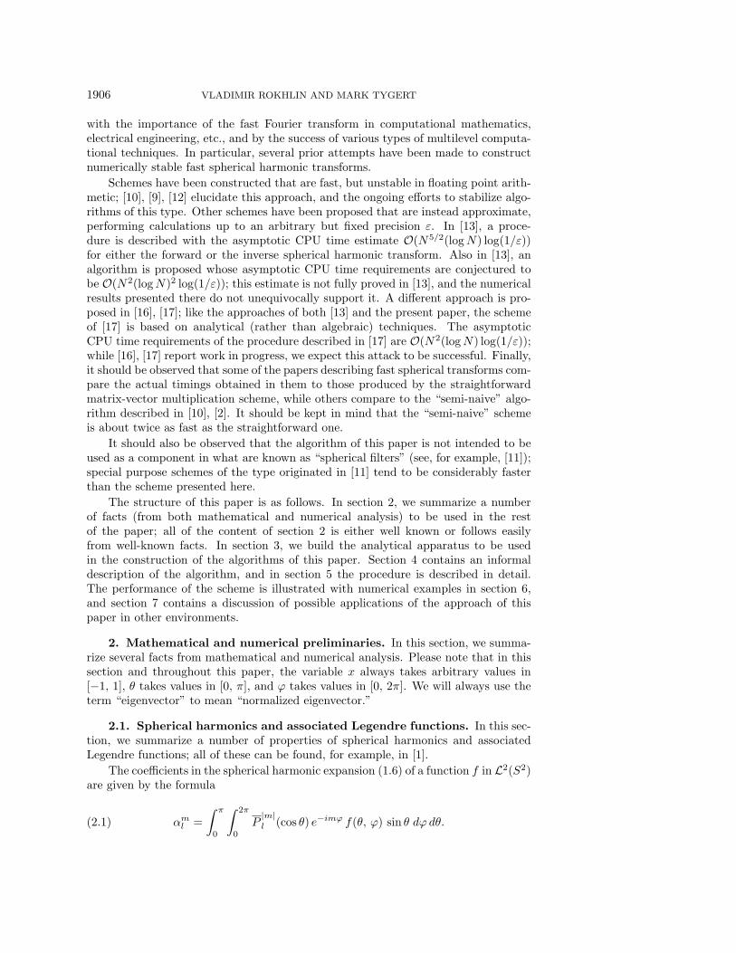
with the importance of the fast Fourier transform in computational mathematics,electrical engineering, etc., and by the success of various types of multilevel computa-tional techniques. In particular, several prior attempts have been made to constructnumerically stable fast spherical harmonic transforms.

Schemes have been constructed that are fast, but unstable in floating point arith-metic; [10], [9], [12] elucidate this approach, and the ongoing efforts to stabilize algo-rithms of this type. Other schemes have been proposed that are instead approximate,performing calculations up to an arbitrary but fixed precision ε. In [13], a proce-dure is described with the asymptotic CPU time estimate O(N5/2(logN) log(1/ε))for either the forward or the inverse spherical harmonic transform. Also in [13], analgorithm is proposed whose asymptotic CPU time requirements are conjectured tobe O(N2(logN)2 log(1/ε)); this estimate is not fully proved in [13], and the numericalresults presented there do not unequivocally support it. A different approach is pro-posed in [16], [17]; like the approaches of both [13] and the present paper, the schemeof [17] is based on analytical (rather than algebraic) techniques. The asymptoticCPU time requirements of the procedure described in [17] are O(N2(logN) log(1/ε));while [16], [17] report work in progress, we expect this attack to be successful. Finally,it should be observed that some of the papers describing fast spherical transforms com-pare the actual timings obtained in them to those produced by the straightforwardmatrix-vector multiplication scheme, while others compare to the “semi-naive” algo-rithm described in [10], [2]. It should be kept in mind that the “semi-naive” schemeis about twice as fast as the straightforward one.

It should also be observed that the algorithm of this paper is not intended to beused as a component in what are known as “spherical filters” (see, for example, [11]);special purpose schemes of the type originated in [11] tend to be considerably fasterthan the scheme presented here.

The structure of this paper is as follows. In section 2, we summarize a numberof facts (from both mathematical and numerical analysis) to be used in the restof the paper; all of the content of section 2 is either well known or follows easilyfrom well-known facts. In section 3, we build the analytical apparatus to be usedin the construction of the algorithms of this paper. Section 4 contains an informaldescription of the algorithm, and in section 5 the procedure is described in detail.The performance of the scheme is illustrated with numerical examples in section 6,and section 7 contains a discussion of possible applications of the approach of thispaper in other environments.

2. Mathematical and numerical preliminaries. In this section, we summa-rize several facts from mathematical and numerical analysis. Please note that in thissection and throughout this paper, the variable x always takes arbitrary values in[−1, 1], θ takes values in [0, π], and ϕ takes values in [0, 2π]. We will always use theterm “eigenvector” to mean “normalized eigenvector.”

2.1. Spherical harmonics and associated Legendre functions. In this sec-tion, we summarize a number of properties of spherical harmonics and associatedLegendre functions; all of these can be found, for example, in [1].

The coefficients in the spherical harmonic expansion (1.6) of a function f in L2(S2)are given by the formula

αml =

∫ π

0

∫ 2π

0

P|m|l (cos θ) e−imϕ f(θ, ϕ) sin θ dϕ dθ.(2.1)


For the forward spherical harmonic transform of order N , we have to compute thecoefficients (2.1) from the values f(θk, ϕj), where θ0, θ1, . . . , θN−1, θN are definedin (1.7), and ϕ0, ϕ1, . . . , ϕ2N−1, ϕ2N are defined in (1.8). For a cost of O(N2 logN),we use the fast Fourier transform to obtain the 2(2N + 1)(N + 1) values gm(θk) andhm(θk) (m = −N , −N + 1, . . . , N − 1, N ; k = 0, 1, . . . , N − 1, N) of the functionsgm and hm defined on [0, π] by the formulae

gm(θ) =

2N∑j=0

cos(mϕj) f(θ, ϕj),(2.2)

hm(θ) =

2N∑j=0

sin(mϕj) f(θ, ϕj).(2.3)

We then evaluate the coefficients (2.1) via the formula

αml =

∫ π

0

P|m|l (cos θ) gm(θ) sin θ dθ − i

∫ π

0

P|m|l (cos θ)hm(θ) sin θ dθ.(2.4)

To evaluate the integrals in (2.4), we have to convert the values fm(cos θk) intothe coefficients pmm, pmm+1, . . . , p

mN−1, p

mN in expansions of functions fm on [−1, 1] of

the form

fm(x) =

N∑l=m

pml Pm

l (x),(2.5)

pml =

∫ 1

−1

Pm

l (x) fm(x) dx,(2.6)

where m is any integer with 0 ≤ m ≤ N .The principal purpose of this paper is the construction of a “fast” scheme for

computing the coefficients (2.6) from the values fm(cos θk), and for computing theinverse of this transformation, that is, for computing the values fm(cos θk) of thefunction fm defined in (2.5) from the coefficients (2.6).

For any nonnegative integers l and m with m ≤ l, the associated Legendre functionPml on [−1, 1] is defined by the formula

Pml (x) = (−1)m

√1 − x2

m dm

dxmPl(x),(2.7)

where Pl is the Legendre polynomial of degree l. Obviously, Pml is a polynomial when

m is even and a polynomial multiplied by√

1 − x2 when m is odd.For any nonnegative integer m, we define the differential operator Lm by the

formula

Lm(f)(x) = − d

dx

((1 − x2)

d

dxf(x)

)+

m2

1 − x2f(x)(2.8)

for any function f on [−1, 1] with a continuous second derivative. For any nonnegativeintegers l and m with m ≤ l, the function P

m

l satisfies the differential equation

Lm

(P

m

l

)(x) = l(l + 1) P

m

l (x),(2.9)


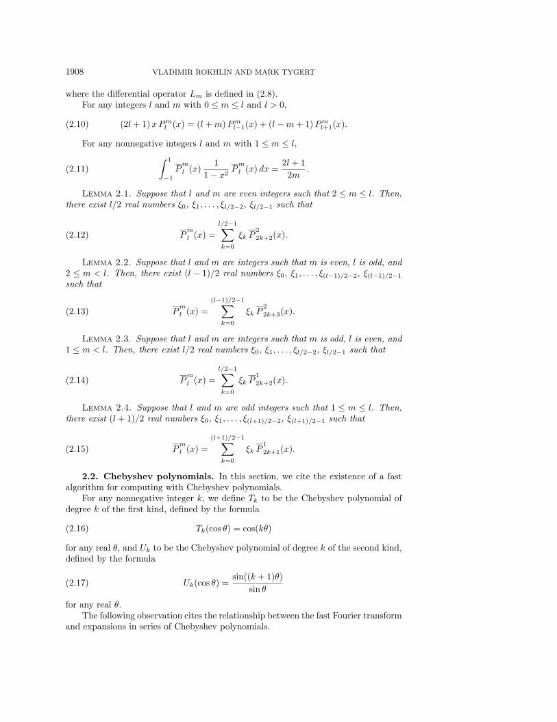
where the differential operator Lm is defined in (2.8).For any integers l and m with 0 ≤ m ≤ l and l > 0,

(2l + 1)xPml (x) = (l + m)Pm

l−1(x) + (l −m + 1)Pml+1(x).(2.10)

For any nonnegative integers l and m with 1 ≤ m ≤ l,∫ 1

−1

Pm

l (x)1

1 − x2P

m

l (x) dx =2l + 1

2m.(2.11)

Lemma 2.1. Suppose that l and m are even integers such that 2 ≤ m ≤ l. Then,there exist l/2 real numbers ξ0, ξ1, . . . , ξl/2−2, ξl/2−1 such that

Pm

l (x) =

l/2−1∑k=0

ξk P2

2k+2(x).(2.12)

Lemma 2.2. Suppose that l and m are integers such that m is even, l is odd, and2 ≤ m < l. Then, there exist (l − 1)/2 real numbers ξ0, ξ1, . . . , ξ(l−1)/2−2, ξ(l−1)/2−1

such that

Pm

l (x) =

(l−1)/2−1∑k=0

ξk P2

2k+3(x).(2.13)

Lemma 2.3. Suppose that l and m are integers such that m is odd, l is even, and1 ≤ m < l. Then, there exist l/2 real numbers ξ0, ξ1, . . . , ξl/2−2, ξl/2−1 such that

Pm

l (x) =

l/2−1∑k=0

ξk P1

2k+2(x).(2.14)

Lemma 2.4. Suppose that l and m are odd integers such that 1 ≤ m ≤ l. Then,there exist (l + 1)/2 real numbers ξ0, ξ1, . . . , ξ(l+1)/2−2, ξ(l+1)/2−1 such that

Pm

l (x) =

(l+1)/2−1∑k=0

ξk P1

2k+1(x).(2.15)

2.2. Chebyshev polynomials. In this section, we cite the existence of a fastalgorithm for computing with Chebyshev polynomials.

For any nonnegative integer k, we define Tk to be the Chebyshev polynomial ofdegree k of the first kind, defined by the formula

Tk(cos θ) = cos(kθ)(2.16)

for any real θ, and Uk to be the Chebyshev polynomial of degree k of the second kind,defined by the formula

Uk(cos θ) =sin((k + 1)θ)

sin θ(2.17)

for any real θ.The following observation cites the relationship between the fast Fourier transform

and expansions in series of Chebyshev polynomials.


Observation 2.5. Suppose that N ≥ 0 is an integer, c0, c1, . . . , cN−1, cN andu0, u1, . . . , uN−1, uN are real numbers, and f and g are the functions on [−1, 1]defined by the formulae

f(x) =N∑

k=0

ck Tk(x),(2.18)

g(x) =N∑

k=0

uk

√1 − x2 Uk(x).(2.19)

Then, there exists an algorithm which uses O(N logN) operations to convert thecoefficients c0, c1, . . . , cN−1, cN into the values f(x0), f(x1), . . . , f(xN−1), f(xN ), andto convert the coefficients u0, u1, . . . , uN−1, uN into the values g(x0), g(x1), . . . , g(xN−1),g(xN ), where the sampling locations x0, x1, . . . , xN−1, xN are defined by the formula

xk = cos

(π(k + 1/2)

N + 1

).(2.20)

Moreover, there exists an algorithm which uses O(N logN) operations to convert thevalues f(x0), f(x1), . . . , f(xN−1), f(xN ) into the coefficients c0, c1, . . . , cN−1, cN , andto convert the values g(x0), g(x1), . . . , g(xN−1), g(xN ) into the coefficients u0, u1, . . . ,uN−1, uN (see, for example, [14]).

2.3. Associated Legendre functions of low orders. In this section, we sum-marize certain simple relationships between Chebyshev polynomials and associatedLegendre functions of orders 1 and 2. These relationships are a straightforward conse-quence of formulae 7.112.1, 8.339.1, 8.339.2, 8.700.1, 8.752.1, 8.826.1, 8.828.1, 8.832.2,and 8.911.4 of [7].

We define the function Λ on [0, ∞) by the formula

Λ(z) =Γ(z + 1/2)

Γ(z + 1),(2.21)

where Γ is the Euler gamma function.For any integer n ≥ 1 and l, k = 0, 1, . . . , n− 2, n− 1, we define the entry An,1,+

l,k

of the n× n matrix An,1,+ by the formulae

An,1,+l,k = − 4l + 3

2(2k + 2l + 3)(2k − 2l − 1)Λ (k − l) Λ

(2k + 2l + 1

2

)(2.22)

×√

4(l + 1)(2l + 1)

4l + 3

when k ≥ l, and

An,1,+l,k = 0(2.23)

otherwise (when k < l).For any integer n ≥ 1 and l, k = 0, 1, . . . , n− 2, n− 1, we define the entry An,1,−

l,k

of the n× n matrix An,1,− by the formulae

An,1,−l,k = − 4l + 5

2(2k + 2l + 5)(2k − 2l − 1)Λ (k − l) Λ

(2k + 2l + 3

2

)(2.24)

×√

4(l + 1)(2l + 3)

4l + 5


when k ≥ l, and

An,1,−l,k = 0(2.25)

otherwise (when k < l).For any integer n ≥ 1 and k, l = 0, 1, . . . , n− 2, n− 1, we define the entry Bn,1,+

k,l

of the n× n matrix Bn,1,+ by the formulae

Bn,1,+k,l = 2

2k + 1

πΛ (l − k) Λ (l + k + 1)

√4l + 3

4(l + 1)(2l + 1)(2.26)

when k ≤ l, and

Bn,1,+k,l = 0(2.27)

otherwise (when k > l).For any integer n ≥ 1 and k, l = 0, 1, . . . , n− 2, n− 1, we define the entry Bn,1,−

k,l

of the n× n matrix Bn,1,− by the formulae

Bn,1,−k,l = 4

k + 1

πΛ (l − k) Λ (l + k + 2)

√4l + 5

4(l + 1)(2l + 3)(2.28)

when k ≤ l, and

Bn,1,−k,l = 0(2.29)

otherwise (when k > l).For any integer n ≥ 1, l = 0, 1, . . . , n − 2, n − 1, and k = 0, 1, . . . , n − 1, n, we

define the entry An,2,+l,k of the n× (n + 1) matrix An,2,+ by the formulae

An,2,+l,k =

(4 +

2k (6(l + 1)(2l + 3) − 2(2k − 1)(2k + 1))

(2k + 2l + 3)(2k − 2l − 3)Λ (k − l − 1)(2.30)

× Λ

(2k + 2l + 1

2

)) √4l + 5

8(l + 1)(l + 2)(2l + 1)(2l + 3)

when k ≥ l + 1, and

An,2,+l,k = 4

√4l + 5

8(l + 1)(l + 2)(2l + 1)(2l + 3)(2.31)

otherwise (when k < l + 1).For any integer n ≥ 1, l = 0, 1, . . . , n − 2, n − 1, and k = 0, 1, . . . , n − 1, n, we

define the entry An,2,−l,k of the n× (n + 1) matrix An,2,− by the formulae

An,2,−l,k =

(4 +

(2k + 1) (6(l + 2)(2l + 3) − 8k(k + 1))

(2k + 2l + 5)(2k − 2l − 3)Λ (k − l − 1)(2.32)

× Λ

(2k + 2l + 3

2

)) √4l + 7

8(l + 1)(l + 2)(2l + 3)(2l + 5)


when k ≥ l + 1, and

An,2,−l,k = 4

√4l + 7

8(l + 1)(l + 2)(2l + 3)(2l + 5)(2.33)

otherwise (when k < l + 1).For any integer n ≥ 1, k = 0, 1, . . . , n − 1, n, and l = 0, 1, . . . , n − 2, n − 1, we

define the entry Bn,2,+k,l of the (n + 1) × n matrix Bn,2,+ by the formulae

Bn,2,+k,l =

2(l + 1)(2l + 3) − 8k2

πΛ (l − k + 1) Λ (l + k + 1)(2.34)

×√

4l + 5

8(l + 1)(l + 2)(2l + 1)(2l + 3)

when k = 0,

Bn,2,+k,l = 2

2(l + 1)(2l + 3) − 8k2

πΛ (l − k + 1) Λ (l + k + 1)(2.35)

×√

4l + 5

8(l + 1)(l + 2)(2l + 1)(2l + 3)

when 0 < k ≤ l + 1, and

Bn,2,+k,l = 0(2.36)

otherwise (when k > l + 1).For any integer n ≥ 1, k = 0, 1, . . . , n − 1, n, and l = 0, 1, . . . , n − 2, n − 1, we

define the entry Bn,2,−k,l of the (n + 1) × n matrix Bn,2,− by the formulae

Bn,2,−k,l =

4(l + 2)(2l + 3) − 4(2k + 1)2

πΛ (l − k + 1) Λ (l + k + 2)(2.37)

×√

4l + 7

8(l + 1)(l + 2)(2l + 3)(2l + 5)

when k ≤ l + 1, and

Bn,2,−k,l = 0(2.38)

otherwise (when k > l + 1).The following four lemmas are proven via mechanical but rather tedious manipu-

lations of formulae 7.112.1, 8.339.1, 8.339.2, 8.700.1, 8.752.1, 8.826.1, 8.828.1, 8.832.2,and 8.911.4 of [7].

The following lemma provides explicit expressions for the matrix Bn,1,+ convert-ing coefficients in linear combinations of associated Legendre functions of order 1 ofodd degrees into coefficients in linear combinations of even Chebyshev polynomials ofthe second kind, scaled by

√1 − x2, and for the matrix An,1,+ converting the latter

into the former.Lemma 2.6. Suppose that n ≥ 1 is an integer, q = (q0, q1, . . . , qn−2, qn−1)

T isa real vector, and f is the function on [−1, 1] defined by the formula

f(x) =

n−1∑l=0

ql P1

2l+1(x).(2.39)


Then,

f(x) =

n−1∑k=0

uk

√1 − x2 U2k(x),(2.40)

where u = (u0, u1, . . . , un−2, un−1)T is the real vector defined by the formula

u = Bn,1,+ q,(2.41)

and Bn,1,+ is defined in (2.21), (2.26), and (2.27). Furthermore,

q = An,1,+ u,(2.42)

where An,1,+ is defined in (2.21), (2.22), and (2.23).The following lemma provides explicit expressions for the matrix Bn,1,− convert-

ing coefficients in linear combinations of associated Legendre functions of order 1 ofeven degrees into coefficients in linear combinations of odd Chebyshev polynomials ofthe second kind, scaled by

√1 − x2, and for the matrix An,1,− converting the latter

into the former.Lemma 2.7. Suppose that n ≥ 1 is an integer, q = (q0, q1, . . . , qn−2, qn−1)

T is areal vector, and f is the function on [−1, 1] defined by the formula

f(x) =n−1∑l=0

ql P1

2l+2(x).(2.43)

Then,

f(x) =n−1∑k=0

uk

√1 − x2 U2k+1(x),(2.44)

where u = (u0, u1, . . . , un−2, un−1)T is the real vector defined by the formula

u = Bn,1,− q,(2.45)

and Bn,1,− is defined in (2.21), (2.28), and (2.29). Furthermore,

q = An,1,− u,(2.46)

where An,1,− is defined in (2.21), (2.24), and (2.25).The following lemma provides explicit expressions for the matrix Bn,2,+ convert-

ing coefficients in linear combinations of associated Legendre functions of order 2 ofeven degrees into coefficients in linear combinations of even Chebyshev polynomialsof the first kind, and for the matrix An,2,+ converting the latter into the former.

Lemma 2.8. Suppose that n ≥ 1 is an integer, p = (p0, p1, . . . , pn−2, pn−1)T is a

real vector, and f is the function on [−1, 1] defined by the formula

f(x) =n−1∑l=0

pl P2

2l+2(x).(2.47)

Then,

f(x) =

n∑k=0

ck T2k(x),(2.48)


where c = (c0, c1, . . . , cn−1, cn)T is the real vector defined by the formula

c = Bn,2,+ p,(2.49)

and Bn,2,+ is defined in (2.21), (2.34), (2.35), and (2.36). Furthermore,

p = An,2,+ c,(2.50)

where An,2,+ is defined in (2.21), (2.30), and (2.31).The following lemma provides explicit expressions for the matrix Bn,2,− convert-

ing coefficients in linear combinations of associated Legendre functions of order 2 ofodd degrees into coefficients in linear combinations of odd Chebyshev polynomials ofthe first kind, and for the matrix An,2,− converting the latter into the former.

Lemma 2.9. Suppose that n ≥ 1 is an integer, p = (p0, p1, . . . , pn−2, pn−1)T is a

real vector, and f is the function on [−1, 1] defined by the formula

f(x) =n−1∑l=0

pl P2

2l+3(x).(2.51)

Then,

f(x) =

n∑k=0

ck T2k+1(x),(2.52)

where c = (c0, c1, . . . , cn−1, cn)T is the real vector defined by the formula

c = Bn,2,− p,(2.53)

and Bn,2,− is defined in (2.21), (2.37), and (2.38). Furthermore,

p = An,2,− c,(2.54)

where An,2,− is defined in (2.21), (2.32), and (2.33).Observation 2.10. Suppose that n ≥ 1 is an integer. Then, there exists an

algorithm which uses O(n log(n/ε)) operations to apply to an arbitrary vector anyof the matrices An,1,+, Bn,1,+, An,1,−, Bn,1,−, An,2,+, Bn,2,+, An,2,−, and Bn,2,−

defined in (2.21)–(2.38), where ε is the precision of computations (see [3]).

2.4. Semiseparable matrices. For any integer n > 0, a semiseparable realn× n matrix S is a matrix whose entry Sj,k is given by the formulae

Sj,k = aj bk(2.55)

when j ≤ k, and

Sj,k = ak bj(2.56)

when j > k, where a = (a0, a1, . . . , an−2, an−1)T and b = (b0, b1, . . . , bn−2, bn−1)

T

are real vectors.Matrices of the form

G = D + S,(2.57)


where D is a diagonal real matrix and S is a semiseparable real matrix, will beencountered repeatedly throughout this paper. The matrix U of eigenvectors of thematrix G in (2.57) will be particularly important; U is orthogonal and diagonalizesG, so that

UT GU = Λ,(2.58)

where Λ is a diagonal real matrix.

The principal numerical tool of this paper is the following observation, made in [8]and [4].

Observation 2.11. The matrices U and UT in (2.58) can be applied to an arbitraryvector of length N for a cost of O(N(logN) log(1/ε)) operations, where ε is theprecision of computations. More precisely, there exists a constant C independent ofN , of ε, and of the particular matrix G in (2.58) such that the matrices U and UT

can be applied for a cost of at most C N(logN) log(1/ε) operations.

Remark 2.12. Strictly speaking, only the numerical apparatus behind Observa-tion 2.11 is constructed in [4]. However, the observation itself is stated explicitly in avery similar environment in [8]. In our implementation, we used a minor modificationof the apparatus in [4], to be reported at a later date.

3. Analytical apparatus. In this section, we construct the principal analyticaltools used in this paper.

In section 3.1, we observe that when the function Pm

l is represented as a lin-

ear combination of functions P1

j or P2

j (depending on whether m is even or odd),the Sturm–Liouville problem (2.9) becomes an eigenvector problem for the matrixG in (2.57). Thus, according to Observation 2.11, there exists an algorithm thatuses O (N(logN) log(1/ε)) operations to apply the matrices U and UT in (2.58) toarbitrary vectors of length N , where ε is the precision of computations.

In section 3.2, we observe that the problem of evaluating expansions of theform (1.12) can be reduced to the problem of evaluating expansions of the forms (1.10)and (1.11), via the matrices U and UT in (2.58). These matrices can be applied toarbitrary vectors efficiently, due to Observation 2.11.

3.1. Associated Legendre differential equations in terms of associatedLegendre functions of low orders. For any even integers n and m with 2 ≤ m ≤ n,and for j, k = 0, 1, . . . , n/2 − 2, n/2 − 1, we define the entry Gn,m

j,k of the n/2 × n/2matrix Gn,m by the formula

Gn,mj,k =

∫ 1

−1

P2

2j+2(x) Lm

(P

2

2k+2

)(x) dx,(3.1)

where the differential operator Lm is defined in (2.8).

For any odd integer n and even integer m with 2 ≤ m < n, and for j, k =0, 1, . . . , (n−1)/2−2, (n−1)/2−1, we define the entry Gn,m

j,k of the (n−1)/2×(n−1)/2matrix Gn,m by the formula

Gn,mj,k =

∫ 1

−1

P2

2j+3(x) Lm

(P

2

2k+3

)(x) dx,(3.2)

where the differential operator Lm is defined in (2.8).


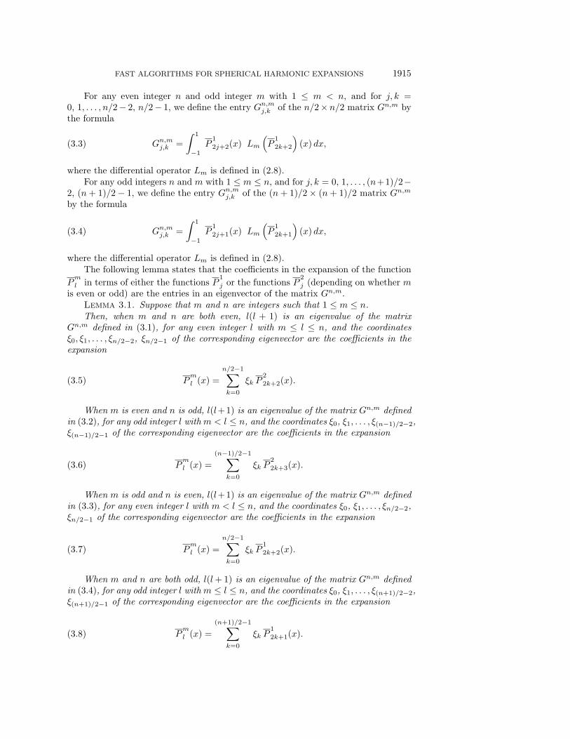
For any even integer n and odd integer m with 1 ≤ m < n, and for j, k =0, 1, . . . , n/2− 2, n/2− 1, we define the entry Gn,m

j,k of the n/2× n/2 matrix Gn,m bythe formula

Gn,mj,k =

∫ 1

−1

P1

2j+2(x) Lm

(P

1

2k+2

)(x) dx,(3.3)

where the differential operator Lm is defined in (2.8).For any odd integers n and m with 1 ≤ m ≤ n, and for j, k = 0, 1, . . . , (n+1)/2−

2, (n + 1)/2 − 1, we define the entry Gn,mj,k of the (n + 1)/2 × (n + 1)/2 matrix Gn,m

by the formula

Gn,mj,k =

∫ 1

−1

P1

2j+1(x) Lm

(P

1

2k+1

)(x) dx,(3.4)

where the differential operator Lm is defined in (2.8).The following lemma states that the coefficients in the expansion of the function

Pm

l in terms of either the functions P1

j or the functions P2

j (depending on whether mis even or odd) are the entries in an eigenvector of the matrix Gn,m.

Lemma 3.1. Suppose that m and n are integers such that 1 ≤ m ≤ n.Then, when m and n are both even, l(l + 1) is an eigenvalue of the matrix

Gn,m defined in (3.1), for any even integer l with m ≤ l ≤ n, and the coordinatesξ0, ξ1, . . . , ξn/2−2, ξn/2−1 of the corresponding eigenvector are the coefficients in theexpansion

Pm

l (x) =

n/2−1∑k=0

ξk P2

2k+2(x).(3.5)

When m is even and n is odd, l(l+1) is an eigenvalue of the matrix Gn,m definedin (3.2), for any odd integer l with m < l ≤ n, and the coordinates ξ0, ξ1, . . . , ξ(n−1)/2−2,ξ(n−1)/2−1 of the corresponding eigenvector are the coefficients in the expansion

Pm

l (x) =

(n−1)/2−1∑k=0

ξk P2

2k+3(x).(3.6)

When m is odd and n is even, l(l+1) is an eigenvalue of the matrix Gn,m definedin (3.3), for any even integer l with m < l ≤ n, and the coordinates ξ0, ξ1, . . . , ξn/2−2,ξn/2−1 of the corresponding eigenvector are the coefficients in the expansion

Pm

l (x) =

n/2−1∑k=0

ξk P1

2k+2(x).(3.7)

When m and n are both odd, l(l + 1) is an eigenvalue of the matrix Gn,m definedin (3.4), for any odd integer l with m ≤ l ≤ n, and the coordinates ξ0, ξ1, . . . , ξ(n+1)/2−2,ξ(n+1)/2−1 of the corresponding eigenvector are the coefficients in the expansion

Pm

l (x) =

(n+1)/2−1∑k=0

ξk P1

2k+1(x).(3.8)


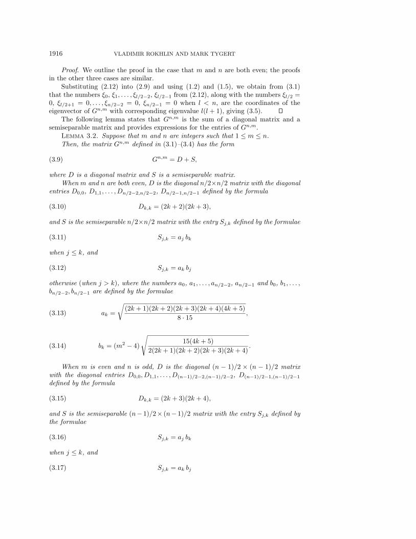
Proof. We outline the proof in the case that m and n are both even; the proofsin the other three cases are similar.

Substituting (2.12) into (2.9) and using (1.2) and (1.5), we obtain from (3.1)that the numbers ξ0, ξ1, . . . , ξl/2−2, ξl/2−1 from (2.12), along with the numbers ξl/2 =0, ξl/2+1 = 0, . . . , ξn/2−2 = 0, ξn/2−1 = 0 when l < n, are the coordinates of theeigenvector of Gn,m with corresponding eigenvalue l(l + 1), giving (3.5).

The following lemma states that Gn,m is the sum of a diagonal matrix and asemiseparable matrix and provides expressions for the entries of Gn,m.

Lemma 3.2. Suppose that m and n are integers such that 1 ≤ m ≤ n.Then, the matrix Gn,m defined in (3.1)–(3.4) has the form

Gn,m = D + S,(3.9)

where D is a diagonal matrix and S is a semiseparable matrix.When m and n are both even, D is the diagonal n/2×n/2 matrix with the diagonal

entries D0,0, D1,1, . . . , Dn/2−2,n/2−2, Dn/2−1,n/2−1 defined by the formula

Dk,k = (2k + 2)(2k + 3),(3.10)

and S is the semiseparable n/2×n/2 matrix with the entry Sj,k defined by the formulae

Sj,k = aj bk(3.11)

when j ≤ k, and

Sj,k = ak bj(3.12)

otherwise (when j > k), where the numbers a0, a1, . . . , an/2−2, an/2−1 and b0, b1, . . . ,bn/2−2, bn/2−1 are defined by the formulae

ak =

√(2k + 1)(2k + 2)(2k + 3)(2k + 4)(4k + 5)

8 · 15,(3.13)

bk = (m2 − 4)

√15(4k + 5)

2(2k + 1)(2k + 2)(2k + 3)(2k + 4).(3.14)

When m is even and n is odd, D is the diagonal (n − 1)/2 × (n − 1)/2 matrixwith the diagonal entries D0,0, D1,1, . . . , D(n−1)/2−2,(n−1)/2−2, D(n−1)/2−1,(n−1)/2−1

defined by the formula

Dk,k = (2k + 3)(2k + 4),(3.15)

and S is the semiseparable (n− 1)/2× (n− 1)/2 matrix with the entry Sj,k defined bythe formulae

Sj,k = aj bk(3.16)

when j ≤ k, and

Sj,k = ak bj(3.17)


otherwise (when j > k), where the numbers a0, a1, . . . , a(n−1)/2−2, a(n−1)/2−1 andb0, b1, . . . , b(n−1)/2−2, b(n−1)/2−1 are defined by the formulae

ak =

√(2k + 2)(2k + 3)(2k + 4)(2k + 5)(4k + 7)

14 · 15,(3.18)

bk = (m2 − 4)

√7 · 15(4k + 7)

8(2k + 2)(2k + 3)(2k + 4)(2k + 5).(3.19)

When m is odd and n is even, D is the diagonal n/2×n/2 matrix with the diagonalentries D0,0, D1,1, . . . , Dn/2−2,n/2−2, Dn/2−1,n/2−1 defined by the formula

Dk,k = (2k + 2)(2k + 3),(3.20)

and S is the semiseparable n/2×n/2 matrix with the entry Sj,k defined by the formulae

Sj,k = aj bk(3.21)

when j ≤ k, and

Sj,k = ak bj(3.22)

otherwise (when j > k), where the numbers a0, a1, . . . , an/2−2, an/2−1 and b0, b1, . . . ,bn/2−2, bn/2−1 are defined by the formulae

ak =

√(2k + 2)(2k + 3)(4k + 5)

30,(3.23)

bk = (m2 − 1)

√15(4k + 5)

2(2k + 2)(2k + 3).(3.24)

When m and n are both odd, D is the diagonal (n + 1)/2 × (n + 1)/2 matrixwith the diagonal entries D0,0, D1,1, . . . , D(n+1)/2−2,(n+1)/2−2, D(n+1)/2−1,(n+1)/2−1

defined by the formula

Dk,k = (2k + 1)(2k + 2),(3.25)

and S is the semiseparable (n+1)/2× (n+1)/2 matrix with the entry Sj,k defined bythe formulae

Sj,k = aj bk(3.26)

when j ≤ k, and

Sj,k = ak bj(3.27)

otherwise (when j > k), where the numbers a0, a1, . . . , a(n+1)/2−2, a(n+1)/2−1 andb0, b1, . . . , b(n+1)/2−2, b(n+1)/2−1 are defined by the formulae

ak =

√(2k + 1)(2k + 2)(4k + 3)

6,(3.28)


bk = (m2 − 1)

√3(4k + 3)

2(2k + 1)(2k + 2).(3.29)

Proof. We outline the proof in the case that m and n are both even; the proofsin the other three cases are similar.

We define the entry Dj,k of the n/2 × n/2 matrix D by the formula

Dj,k =

∫ 1

−1

P2

2j+2(x) L2

(P

2

2k+2

)(x) dx,(3.30)

where the differential operator L2 is defined in (2.8), and we define the entry Sj,k ofthe n/2 × n/2 matrix S by the formula

Sj,k =

∫ 1

−1

P2

2j+2(x)m2 − 4

1 − x2P

2

2k+2(x) dx.(3.31)

We now show that Gn,m = D + S, D is diagonal, and S is semiseparable.Combining (3.1), (3.30), (3.31), and (2.8), we obtain the decomposition (3.9).Substituting (2.9) into (3.30), and using (1.2) and (1.5), we observe that the

matrix D is diagonal with the diagonal entries given by (3.10).In order to obtain the formulae (3.11)–(3.14), we define the entry Mj,k of the

infinite-dimensional matrix M , for j, k = 0, 1, 2, . . . , by the formula

Mj,k =

∫ 1

−1

P2

2j+2(x)m2 − 4

1 − x2P

2

2k+2(x) dx(3.32)

and observe that the entry (M−1)j,k of the inverse M−1 of the matrix M is given bythe formula

(M−1)j,k =

∫ 1

−1

P2

2j+2(x)1 − x2

m2 − 4P

2

2k+2(x) dx,(3.33)

since M represents the operator acting on functions on [−1, 1] by multiplication bythe factor

m2 − 4

1 − x2,(3.34)

whereas M−1 represents the operator acting on functions on [−1, 1] by multiplicationby the inverse factor

1 − x2

m2 − 4.(3.35)

Using (1.2), (1.5), (2.10), and (3.33), we observe that M−1 is tridiagonal. So, Mis the inverse of a tridiagonal matrix, and, as such, M is semiseparable (see, forexample, [6]). But, for j, k = 0, 1, . . . , n/2 − 2, n/2 − 1, (3.31) and (3.32) show thatSj,k = Mj,k, so that S is also semiseparable.

Integrating by parts a few times, while using (1.2), (1.5), and (2.7), together withthe definition (3.31), yields explicit expressions for the uppermost entries S0,0, S0,1, . . . ,S0,n/2−2, S0,n/2−1 of S. Combining (1.2), (1.5), (2.11), and (3.31) yields explicit ex-pressions for the diagonal entries S0,0, S1,1, . . . , Sn/2−2,n/2−2, Sn/2−1,n/2−1 of S. Com-bining all of these explicit expressions with the fact that S is semiseparable, we obtainthe formulae (3.11)–(3.14).


3.2. Associated Legendre expansions of arbitrary orders and associatedLegendre expansions of low orders. Lemmas 3.3, 3.4, 3.5, and 3.6 of this sectionfollow immediately from Lemma 3.1.

Lemma 3.3 states that the matrix of eigenvectors of the matrix Gn,m in (3.9)converts the coefficients in the expansion of a function f in terms of the functionsP

m

m, Pm

m+2, . . . , Pm

n−2, Pm

n into the coefficients in the expansion of the function f in

terms of the functions P2

2, P2

4, . . . , P2

n−2, P2

n. Lemma 3.3 states, moreover, that theadjoint of the matrix of eigenvectors converts the latter coefficients into the formercoefficients.

Lemma 3.3. Suppose that n and m are even integers such that 2 ≤ m ≤ n,pm = (pm0 , pm1 , . . . , pmn/2−2, p

mn/2−1)

T is a real column vector such that pm(n−m)/2+1 =0, pm(n−m)/2+2 = 0, . . . , pmn/2−2 = 0, pmn/2−1 = 0, and f is the function defined on

[−1, 1] by the formula

f(x) =

(n−m)/2∑j=0

pmj Pm

2j+m(x).(3.36)

Then,

f(x) =

n/2−1∑l=0

p2l P

2

2l+2(x),(3.37)

where p2 = (p20, p

21, . . . , p

2n/2−2, p

2n/2−1)

T is the real vector defined by the formula

p2 = U pm,(3.38)

and U is an n/2× n/2 matrix of eigenvectors of the symmetric matrix Gn,m in (3.9)with

Pm

2j+m(x) =

n/2−1∑l=0

Ul,j P2

2l+2(x)(3.39)

for j = 0, 1, . . . , (n−m)/2 − 1, (n−m)/2. Moreover,

pm = UT p2.(3.40)

Lemmas 3.4, 3.5, and 3.6 are analogues of Lemma 3.3 for different conditions onm and n.

Lemma 3.4. Suppose that n and m are integers such that m is even, n is odd,2 ≤ m < n, pm = (pm0 , pm1 , . . . , pm(n−5)/2, p

m(n−3)/2)

T is a real column vector such thatpm(n−m+1)/2 = 0, pm(n−m+3)/2 = 0, . . . , pm(n−5)/2 = 0, pm(n−3)/2 = 0, and f is the function

defined on [−1, 1] by the formula

f(x) =

(n−m−1)/2∑j=0

pmj Pm

2j+m+1(x).(3.41)

Then,

f(x) =

(n−3)/2∑l=0

p2l P

2

2l+3(x),(3.42)


where p2 = (p20, p

21, . . . , p

2(n−5)/2, p

2(n−3)/2)


p2 = U pm,(3.43)

and U is an (n − 1)/2 × (n − 1)/2 matrix of eigenvectors of the symmetric matrixGn,m in (3.9) with

Pm

2j+m+1(x) =

(n−3)/2∑l=0

Ul,j P2

2l+3(x)(3.44)

for j = 0, 1, . . . , (n−m− 3)/2, (n−m− 1)/2. Moreover,

pm = UT p2.(3.45)

Lemma 3.5. Suppose that n and m are integers such that m is odd, n is even,1 ≤ m < n, pm = (pm0 , pm1 , . . . , pmn/2−2, p

mn/2−1)

T is a real column vector such thatpm(n−m+1)/2 = 0, pm(n−m+3)/2 = 0, . . . , pmn/2−2 = 0, pmn/2−1 = 0, and f is the function

defined on [−1, 1] by the formula

f(x) =

(n−m−1)/2∑j=0

pmj Pm

2j+m+1(x).(3.46)

Then,

f(x) =

n/2−1∑l=0

p1l P

1

2l+2(x),(3.47)

where p1 = (p10, p

11, . . . , p

1n/2−2, p

1n/2−1)


p1 = U pm,(3.48)

and U is an n/2× n/2 matrix of eigenvectors of the symmetric matrix Gn,m in (3.9)with

Pm

2j+m+1(x) =

n/2−1∑l=0

Ul,j P1

2l+2(x)(3.49)

for j = 0, 1, . . . , (n−m− 3)/2, (n−m− 1)/2. Moreover,

pm = UT p1.(3.50)

Lemma 3.6. Suppose that n and m are odd integers such that 1 ≤ m ≤ n,pm = (pm0 , pm1 , . . . , pm(n−3)/2, p

m(n−1)/2)

T is a real column vector such that pm(n−m)/2+1 =0, pm(n−m)/2+2 = 0, . . . , pm(n−3)/2 = 0, pm(n−1)/2 = 0, and f is the function defined on

[−1, 1] by the formula

f(x) =

(n−m)/2∑j=0

pmj Pm

2j+m(x).(3.51)


Then,

f(x) =

(n−1)/2∑l=0

p1l P

1

2l+1(x),(3.52)

where p1 = (p10, p

11, . . . , p

1(n−3)/2, p

1(n−1)/2)


p1 = U pm,(3.53)

and U is an (n + 1)/2 × (n + 1)/2 matrix of eigenvectors of the symmetric matrixGn,m in (3.9) with

Pm

2j+m(x) =

(n−1)/2∑l=0

Ul,j P1

2l+1(x)(3.54)

for j = 0, 1, . . . , (n−m)/2 − 1, (n−m)/2. Moreover,

pm = UT p1.(3.55)

4. Informal description of the algorithm. In this section, we outline a “fast”algorithm for the conversion of the values f0, f1, . . . , fN−1, fN of the function ftabulated at the nodes x0, x1, . . . , xN−1, xN , defined by the formula

xk = cos

(π(k + 1/2)

N + 1

),(4.1)

into the coefficients p0, p1, . . . , pN−m−1, pN−m in the expansion

f(x) =

N−m∑l=0

pl Pm

l+m(x).(4.2)

(The inverse procedure of converting the coefficients p0, p1, . . . , pN−m−1, pN−m intothe values f0, f1, . . . , fN−1, fN is quite similar, so we omit its description.)

The procedure consists of four steps, described briefly below. Since the procedurewhen m is odd is virtually the same as when m is even, we describe the procedureonly for the case that m is even. For definitiveness, we assume also that N is even.

Step 1. We separate f into its even and odd parts f+ and f−, defined by theformulae

f+(x) =f(x) + f(−x)√

2,(4.3)

f−(x) =f(x) − f(−x)√

2.(4.4)

All subsequent processing is performed separately for f+ and f−. Since the proceduresfor f+ and f− are virtually identical, we describe only the procedure for the even partf+.

Step 2. Using the fast Fourier transform as in Observation 2.5, we convert thevalues f+

0 , f+1 , . . . , f+

N−1, f+N of the function f+, defined in (4.3), at the points x0, x1,


. . . , xN−1, xN , defined in (4.1), into the coefficients c0, c1, . . . , cN/2−1, cN/2 in theexpansion

f+(x) =

N/2∑k=0

ck T2k(x).(4.5)

Step 3. Using Lemma 2.8 and Observation 2.10, we convert the coefficientsc0, c1, . . . , cN/2−1, cN/2 in the expansion (4.5) into the coefficients p2

0, p21, . . . , p

2N/2−2,

p2N/2−1 in the expansion

f+(x) =

N/2−1∑l=0

p2l P

2

2l+2(x).(4.6)

Step 4. Using Lemmas 3.2 and 3.3 and Observation 2.11, we convert the coeffi-cients p2

0, p21, . . . , p2

N/2−2, p2N/2−1 in the expansion (4.6) into the coefficients pm0 , pm1 ,

. . . , pm(N−m)/2−1, pm(N−m)/2 in the expansion

f+(x) =

(N−m)/2∑l=0

pml Pm

2l+m(x).(4.7)

Remark 4.1. Clearly, Step 1 takes O(N) operations. As per Observation 2.5, Step2 takes O(N logN) operations. As per Observation 2.10, Step 3 takes O(N log(N/ε))operations, where ε is the precision of computations. As per Observation 2.11, Step 4takes O(N(logN) log(1/ε)) operations, where ε is the precision of computations usedin this step. All together, Steps 1–4 take O(N(logN) log(1/ε)) operations.

Remark 4.2. To handle f− when m is even, we substitute Lemma 2.9 forLemma 2.8 in Step 3 and Lemma 3.4 for Lemma 3.3 in Step 4. For f− when mis even, we find that p2

N/2−1 = 0 and cN/2 = 0, since, when m is even, f− is a linear

combination of only N/2 − 1 functions P2

3, P2

5, . . . , P2

N−3, P2

N−1 (or, equivalently, ofthe N/2 Chebyshev polynomials of the first kind T1, T3, . . . , TN−3, TN−1).

To handle f+ when m is odd, we substitute Lemma 2.6 for Lemma 2.8 in Step 3and Lemma 3.6 for Lemma 3.3 in Step 4.

To handle f− when m is odd, we substitute Lemma 2.7 for Lemma 2.8 in Step 3and Lemma 3.5 for Lemma 3.3 in Step 4.

When computing the coefficients (2.1) in the spherical harmonic expansion (1.6),we tabulate the function f on [−1, 1] at the same N+1 sampling locations x0, x1, . . . ,xN−1, xN when m is odd as when m is even, even though when m is odd, f is

a linear combination of only N functions P1

1, P1

2, . . . , P1

N−1, P1

N (or, equivalently,

of the N Chebyshev polynomials of the second kind√

1 − x2 U0,√

1 − x2 U1, . . . ,√1 − x2 UN−2,

√1 − x2 UN−1, which are scaled by

√1 − x2).

5. Detailed description of the algorithm. In this section, we describe indetail the algorithm described informally in section 4.

Precomputations.

Comment [Compute all the data that Steps 3 and 4 require that do not dependon f .]Compute all the data that Step 3 requires to apply fast the matrix AN/2,2,+

from Lemma 2.8 (i.e., “compress” the matrix AN/2,2,+).


Compute all the data that Step 4 requires to apply fast the adjoint of thematrix U from Lemmas 3.2 and 3.3 (i.e., “compress” the matrix UT).

Step 1.

Comment [Convert the values f0, f1, . . . , fN−1, fN into the values f+0 , f+

1 , . . . ,f+N−1, f

+N .]

do n = 0, . . . , NSet f+

n = (fn + fN−n)/√

2.enddo

Step 2.

Comment [Convert the values f+0 , f+

1 , . . . , f+N−1, f

+N into the coefficients c0, c1, . . . ,

cN/2−1, cN/2 of the Chebyshev polynomials T0, T2, . . . , TN−2, TN .]Use the discrete cosine transform (see, for example, [14]) to convert the valuesf+0 , f+

1 , . . . , f+N−1, f

+N into the coefficients c0, c1, . . . , cN/2−1, cN/2.

Step 3.

Comment [Convert the coefficients c0, c1, . . . , cN/2−1, cN/2 of the Chebyshev poly-nomials T0, T2, . . . , TN−2, TN into the coefficients p2

0, p21, . . . , p

2N/2−2, p

2N/2−1

of the associated Legendre functions P2

2, P2

4, . . . , P2

N−2, P2

N .]

Use Observation 2.10 to apply the matrix AN/2,2,+ from Lemma 2.8 to thevector c = (c0, c1, . . . , cN/2−1, cN/2)

T, in order to obtain the vector p2 =(p2

0, p21, . . . , p

2N/2−2, p

2N/2−1)

T.

Step 4.

Comment [Convert the coefficients p20, p

21, . . . , p

2N/2−2, p

2N/2−1 of the associated

Legendre functions P2

2, P2

4, . . . , P2

N−2, P2

N of order 2 into the coefficientspm0 , pm1 , . . . , pm(N−m)/2−1, pm(N−m)/2 of the associated Legendre functions

Pm

m, Pm

m+2, . . . , Pm

N−2, Pm

N .]

Use Observation 2.11 to apply the adjoint of the matrix U from Lemmas 3.2and 3.3 to the vector p2 = (p2

0, p21, . . . , p

2N/2−2, p

2N/2−1)

T, in order to obtain

the vector pm = (pm0 , pm1 , . . . , pmN/2−2, pmN/2−1)

T.

Comment [Only the first (N−m)/2+1 entries of pm interest us; the other entriesvanish: pm(N−m)/2+1 = 0, pm(N−m)/2+2 = 0, . . . , pmN/2−2 = 0, pmN/2−1 = 0.]

6. Numerical results. The algorithms described in this paper have been im-plemented in Fortran. Tables 1–8 report the results of applying the algorithm tofunctions f defined on [−1, 1] by the formulae

f(x) =

(N−m)/2∑l=0

εl Pm

2l+m(x)(6.1)

when m is even and degrees are even,

f(x) =

(N−m−2)/2∑l=0

εl Pm

2l+m+1(x)(6.2)

when m is even and degrees are odd,

f(x) =

(N−m−1)/2∑l=0

εl Pm

2l+m+1(x)(6.3)


Table 1

Times in seconds and errors for m = N+62

, even degrees, reconstruction.

N m“Fast” trans-

formationThird of applyingan N

2×N

2matrix

Precomp-utation

Relativer.m.s. error

1024 515 .20E−02 .91E−03 .20E+01 .64E−072048 1027 .52E−02 .36E−02 .80E+01 .58E−074096 2051 .23E−01 .15E−01 .33E+02 .17E−068192 4099 .48E−01 .58E−01 .16E+03 .39E−0616384 8195 .11E+00 .23E+00 .69E+03 .72E−0632768 16387 .24E+00 .96E+00 .36E+04 .14E−0565536 32771 .51E+00 (.37E+01) .14E+05 .52E−06131072 65539 .11E+01 (.15E+02) .63E+05 .70E−05

Table 2

Times in seconds and errors for m = N+62

, even degrees, decomposition.



2×N

2matrix

Precomp-utation



Table 3

Times in seconds and errors for m = N−42

, even degrees, reconstruction.



2×N

2matrix

Precomp-utation



Table 4


, even degrees, decomposition.



2×N

2matrix

Precomp-utation




Table 5


, odd degrees, reconstruction.



2×N

2matrix

Precomp-utation


1024 31 .16E−02 .91E−03 .20E+01 .86E−082048 63 .43E−02 .36E−02 .70E+01 .20E−074096 127 .20E−01 .15E−01 .28E+02 .16E−068192 255 .43E−01 .58E−01 .11E+03 .41E−0616384 511 .94E−01 .23E+00 .56E+03 .60E−0632768 1023 .21E+00 .96E+00 .26E+04 .10E−0565536 2047 .46E+00 (.37E+01) .14E+05 .14E−05131072 4095 .10E+01 (.15E+02) .47E+05 .14E−05

Table 6


, odd degrees, decomposition.



2×N

2matrix

Precomp-utation


1024 31 .15E−02 .91E−03 .20E+01 .71E−082048 63 .41E−02 .36E−02 .70E+01 .59E−084096 127 .20E−01 .15E−01 .27E+02 .82E−088192 255 .42E−01 .58E−01 .12E+03 .76E−0816384 511 .92E−01 .23E+00 .55E+03 .12E−0732768 1023 .21E+00 .96E+00 .25E+04 .13E−0765536 2047 .45E+00 (.37E+01) .11E+05 .11E−07131072 4095 .98E+00 (.15E+02) .46E+05 .20E−07

Table 7

Times in seconds and errors for m = 15N16

, odd degrees, reconstruction.



2×N

2matrix

Precomp-utation



Table 8

Times in seconds and errors for m = 15N16

, odd degrees, decomposition.



2×N

2matrix

Precomp-utation




when m is odd and degrees are even, and

f(x) =

(N−m−1)/2∑l=0

εl Pm

2l+m(x)(6.4)

when m is odd and degrees are odd; ε0, ε1, ε2, . . . are randomly generated numbers inthe interval [−1, 1]. The decomposition algorithm computes from the sample valuesof f the coefficients in the representation of f as a linear combination of the functionsP

m

m, Pm

m+1, . . . , Pm

N−1, Pm

N ; the reconstruction algorithm computes the sample valuesof f from the coefficients in the representation of f as a linear combination of thefunctions P

m

m, Pm

m+1, . . . , Pm

N−1, Pm

N . The CPU times are in seconds. The errors arerelative root-mean-square errors.

The columns labeled “ ‘fast’ transformation” list the times taken by the algorithmto evaluate one sum of the form (6.1), (6.2), (6.3), or (6.4).

The columns labeled “third of applying an N2 × N

2 matrix” list the times, divided

by 3, taken to apply an N2 × N

2 matrix once to a vector of length N2 . These times scale

quadratically with N ; the figures in parentheses are estimates used when the memoryrequired by direct calculations would be excessive.

Remark 6.1. The columns labeled “third of applying an N2 × N

2 matrix” givesome indication of how much time current implementations of the decompositionsand reconstructions take to run; these times are believed to be reasonable estimatesof how a standard package like Spherepack (see [2], [18]) would perform, using the“semi-naive” algorithm described in [10], for example. Clearly, for sufficiently small N ,the “slow” implementation would actually run faster than the “fast” implementation.

The code was compiled with the Lahey–Fujitsu compiler, with optimization flag--o2, and run on a 2.8 GHz Intel Pentium Xeon microprocessor with 512 KB of L2cache.

No effort was made to optimize the precomputations. To simplify the imple-mentation, precomputations that take O(N2) operations were used, even though thetechniques described in [4] lead naturally to precomputations that would take onlyO(N logN) operations. The precomputations were run to yield approximately 6 dig-its of accuracy, running all computations (including the precomputations) in doubleprecision arithmetic.

Observation 6.2. Asymptotically, the algorithm should require a number of oper-ations proportional to N(logN) log(1/ε) to evaluate one sum of the form (6.1), (6.2),(6.3), or (6.4), where ε ≈ 10−6. The times in the columns labeled “ ‘fast’ transfor-mation” appear to be consistent with this estimate. The algorithm appears to breakeven with standard matrix multiplication methods for computing spherical harmonicexpansions between N = 4096 and N = 8192; however, no serious effort has beenmade to optimize our implementation.

7. Generalizations. The algorithm of this paper admits a number of general-izations and extensions. The following list is not intended to be exhaustive; subjectsin it are under investigation, and these investigations will be reported at a later date.

1. Different discretizations of S2. Throughout this paper, we have assumedthat the meridians on S2 are discretized in an equispaced manner, i.e., that thepoints θ0, θ1, . . . , θN−1, θN subdivide the interval [0, π] into equal subintervals. Thislimitation is easily removed via techniques described in [11], [19], and [5]; however, tomaintain numerical stability, the nodes have to satisfy certain quite restrictive criteria.One important collection of nodes that does in fact lead to stable algorithms is given


by the formula

θk = cos−1(xk),(7.1)

where x0, x1, . . . , xN−1, xN are Gaussian nodes on the interval [−1, 1] (see, for ex-ample, [2]).

Furthermore, the nodes ϕ0, ϕ1, . . . , ϕ2N−1, ϕ2N in the discretizations of the par-allels on S2 do not have to be equispaced, provided some form of nonequispacedfast Fourier transform is used; again, numerical stability requires that ϕ0, ϕ1, . . . ,ϕ2N−1, ϕ2N be fairly close to being equispaced.

2. Associated Laguerre functions. Associated Laguerre functions are definedon the entire half-line [0, ∞), but are very small outside of a finite interval. TheSturm–Liouville problem that generates the associated Laguerre functions becomesan eigenvector problem for the sum of a diagonal matrix and a semiseparable matrixwhen discretized using associated Laguerre functions of low orders (very much likethe associated Legendre functions).

3. Prolate spheroidal wave functions. The Sturm–Liouville problem that gen-erates the prolate spheroidal wave functions becomes an eigenvector problem for atridiagonal matrix when discretized using Legendre polynomials.

4. Associated prolate spheroidal wave functions. The Sturm–Liouville problemthat generates the associated prolate spheroidal wave functions becomes an eigenvec-tor problem for the sum of a tridiagonal matrix and a semiseparable matrix whendiscretized using associated Legendre functions of low orders.

Acknowledgments. The authors would like to thank R. R. Coifman for manyuseful and inspiring discussions, and P. N. Swarztrauber, M. J. Mohlenkamp, and thereferees for several suggestions that have improved the exposition.

REFERENCES

[1] M. Abramowitz and I. Stegun, eds., Handbook of Mathematical Functions, Dover, NewYork, 1972.

[2] J. C. Adams and P. N. Swarztrauber, SPHEREPACK 3.0: A model development facility,Mon. Wea. Rev., 127 (1999), pp. 1872–1878.

[3] B. Alpert and V. Rokhlin, A fast algorithm for the evaluation of Legendre expansions, SIAMJ. Sci. Statist. Comput., 12 (1991), pp. 158–179.

[4] S. Chandrasekaran and M. Gu, A divide-and-conquer algorithm for the eigendecomposi-tion of symmetric block-diagonal plus semiseparable matrices, Numer. Math., 96 (2004),pp. 723–731.

[5] A. Dutt, M. Gu, and V. Rokhlin, Fast algorithms for polynomial interpolation, integration,and differentiation, J. Numer. Anal., 33 (1996), pp. 1689–1711.

[6] F. R. Gantmacher and M. G. Krein, Oscillation Matrices and Small Vibrations of Mechan-ical Systems, revised English ed., AMS Chelsea Publishing, Providence, RI, 2002.

[7] I. S. Gradshteyn and I. M. Ryzhik, Tables of Integrals, Series, and Products, 6th ed., Aca-demic Press, San Diego, CA, 2000.

[8] M. Gu and S. C. Eisenstat, A divide-and-conquer algorithm for the symmetric tridiagonaleigenproblem, SIAM J. Matrix Anal. Appl., 16 (1995), pp. 172–191.

[9] D. M. Healy, P. J. Kostelec, and D. Rockmore, Towards safe and effective high-orderLegendre transforms with applications to FFTs for the 2-sphere, Adv. Comput. Math., 21(2004), pp. 59–105.

[10] D. M. Healy, P. J. Kostelec, D. Rockmore, and S. S. B. More, FFTs for the 2-sphere—Improvements and variations, J. Fourier Anal. Appl., 9 (2003), pp. 341–385.

[11] R. Jacob-Chien and B. Alpert, A fast spherical filter with uniform resolution, J. Comput.Phys., 136 (1997), pp. 580–584.

[12] S. Kunis and D. Potts, Fast spherical Fourier algorithms, J. Comput. Appl. Math., 161(2003), pp. 75–98.


[13] M. J. Mohlenkamp, A fast transform for spherical harmonics, J. Fourier Anal. Appl., 5 (1999),pp. 159–184.

[14] W. H. Press, S. A. Teukolsky, W. T. Vetterling, and B. P. Flannery, Numerical Recipesin Fortran 77, 2nd ed., Cambridge University Press, Cambridge, UK, 1992.

[15] V. Rokhlin and M. Tygert, Fast Algorithms for Spherical Harmonic Expansions, Technicalreport 1309, Department of Computer Science, Yale University, New Haven, CT, 2004.

[16] R. Suda, Stability analysis of the fast Legendre transform algorithm based on the fast multipolemethod, Proc. Estonian Acad. Sci. Phys. Math., 53 (2004), pp. 107–115.

[17] R. Suda and M. Takami, A fast spherical harmonics transform algorithm, Math. Comp., 71(2002), pp. 703–715.

[18] P. N. Swarztrauber and W. F. Spotz, Generalized discrete spherical harmonic transforms,J. Comput. Phys., 159 (2000), pp. 213–230.

[19] N. Yarvin and V. Rokhlin, A generalized one-dimensional fast multipole method with appli-cation to filtering of spherical harmonics, J. Comput. Phys., 147 (1998), pp. 594–609.

1. introduction. - tygert

Documents