1

Real-time Exploration and Photorealistic

Reconstruction of Large Natural Environments

Nikos Komodakis and Georgios Tziritas

Computer Science Department, University of Crete

E-mails: {komod, tziritas}@csd.uoc.gr

Abstract

This paper presents a hybrid (geometry- & image-based) framework suitable for providing photorealistic

walkthroughs of large, complex outdoor scenes, based only on a small set of real images from the scene. To

this end, a novel data representation of a 3D scene is proposed, which is called morphable 3D-mosaics. Mo-

tion is assumed to be taking place along a predefined path of the 3D environment and the input to the system

is a sparse set of stereoscopic views at certain positions (key-positions) along that path (one view per posi-

tion). An approximate local 3D model is constructed from each view, capable of capturing the photometric

and geometric properties of the scene only locally. Then during the rendering process, a continuous morphing

(both photometric as well as geometric) takes place between successive local 3D models, using what we call

a “morphable 3D-model”. For the estimation of the photometric morphing, a robust algorithm capable of

extracting a dense field of 2D correspondences between wide-baseline images is used, whereas for the geo-

metric morphing, a novel method of computing 3D correspondences between local models is proposed. This

way, a physically-valid morphing is always produced, which is thus kept transparent from the user. Moreover,

a highly optimized rendering path is being used during morphing, which thus allows for high frame rates.

Our system can be extended to handle multiple stereoscopic views (and therefore multiple local models)

per key-position of the path (related by a camera rotation). In this case, one local 3D-mosaic (per key-

position) is constructed, comprising all local 3D models therein, and so a “morphable 3D-mosaic” is now

used during the rendering process. For handling the geometric consistency of each 3D-mosaic, a technique

which is based on solving a partial differential equation is adopted. The effectiveness of our framework is

demonstrated by using it for the 3D visual reconstruction of the Samaria Gorge in Crete.

I. INTRODUCTION

One research problem of computer graphics that has attracted a lot of attention over the last years

is the creation of modeling and rendering systems capable to provide photorealistic & interactive

2

t, λ

Fig. 1: A schematic view of the plenoptic function

walkthroughs of complex, real-world environments. Two are the main approaches that have been

proposed so far for that purpose. On one hand, there exist those techniques that are geometry-based.

These work by first trying to estimate an accurate global 3D model of the scene. They then use the

extracted 3D model in order to render the scene under any given viewpoint. One of their advantages

is that they provide great flexibility and allow many of the scene’s properties to be modified during

rendering. E.g. by having a global 3D model one can readily alter not only the viewpoint but also the

lighting conditions of the scene. However, their big disadvantage comes from the fact that extracting

an accurate global 3D model can be either extremely time consuming or very difficult (not to say

impossible) in many cases. For example such a 3D-model construction task can be easy for scenes

containing mostly planar objects (e.g. architectural-type scenes) but becomes extremely hard for

outdoor scenes containing objects with irregular geometry e.g. trees. The automatic extraction of

a 3D-model from images, also known as multiple view geometry, has been (and still is) an active

research topic in computer vision. In fact a significant amount of progress has been achieved in

this area over the last years [1]–[3].

A second class of techniques that has emerged during the last years are the so-called Image Based

Rendering (IBR) methods [4]. These techniques concentrate their effort directly on how to fill the

pixels of a novel view and skip the geometric modeling of the scene completely. In place of the

geometric modeling, a dense set of images inside the scene is captured as a first step. One then tries

to synthesize any given view by appropriately resampling the previously acquired set of captured

images. By thinking of the world’s appearance as a dense array of light rays filling the space, one

can easily see that what all image based rendering methods actually try to do is to reconstruct

the so-called plenoptic function [5]. This is a 7-dimensional function P (Vx, Vy, Vz, θ, φ, λ, t) which

models a 3D dynamic environement by recording the light rays at every space location (Vx, Vy, Vz),

towards every possible direction (θ, φ), over any range of wavelengths λ and at any time t (see

Figure 1). Each time we capture an image by a camera, the light rays passing through the camera’s

3

stereoscopic views local 3D models

L1

L3L2

key-positions

pos1

pos3

pos2

a b c

L3L1 L2Lmorph

morphable 3D model

Fig. 2: (a) A sparse set of stereoscopic views is captured at key-positions along the path (b) One local 3D modelis constructed out of each stereoscopic view (c) As the user traverses the path a morphable 3D model is displayedduring rendering. This way, a continuous morphing between successive local models takes place at any time, with thismorphing being both photometric as well as geometric.

center of projection are recorded and so that image can be considered as a specific sample of the

plenoptic function. Based on these observations, image based rendering can thus be thought of

as the signal processing task of reconstructing a continuous functions (in this case the plenoptic

function) based only on a discrete set of samples from that function. As IBR methods make use of

actual images from the scene under consideration, one of their greatest advantages is the fact that

they can attain high levels of photorealism . However, this comes at the price of requiring a big

number of captured images. This actually forms one of the biggest problem of IBR methods and

is the main reason that the great majority of existing IBR techniques can be applied only to scenes

of either small or medium scale. If one tries to apply such techniques to large scale scenes, then

he is confronted with a huge amount of data required which makes these methods impractical for

such cases.

So, while a lot of research has been done regarding small scale scenes, there are only few

examples of work dealing with large scale environments. The presented framework [6], [7] is such

an example of a hybrid (geometry and image based) approach, capable of providing photorealistic

and interactive walkthroughs of large-scale, complex outdoor environments, using as input only a

small set of images from the scene. To this end, one major contribution of this work is the proposal

of a novel data representation for a 3D scene, called morphable 3D-mosaics, consisting of a series

of morphable (both geometrically as well as photometrically) 3D models. The main assumption is

that during the walkthrough, the user motion takes place along a (relatively) smooth, predefined

path of the environment. The input to our system is then a sparse set of stereoscopic views captured

at certain locations (which we will call “key-positions” hereafter) along that path (see Figure 2a).

Assuming initially that only one view per key-position exists, a series of local 3D models are then

constructed, one for each stereoscopic view, with these local models capturing the photometric and

4

geometric properties of the scene at a local level and containing only an approximate representation

of the scene’s geometry (see Figure 2b). Then, instead of trying to create a global 3D model out

of all these local models (a task that can prove to be extremely difficult in many cases, requiring

a very accurate registration between local models), we rather follow a different approach. The key

idea is that during the transition between any two successive key-positions (say pos1, pos2) along

the path, a “morphable 3D-model” Lmorph is displayed by the rendering process (see Figure 2c).

At position pos1 this model coincides with the local model L1 at that position, while as we are

approaching pos2 it is gradually transformed into the next local model L2, coinciding with that

upon reaching key-position pos2. Therefore, during the rendering process, and as the user traverses

the predefined path, a continuous morphing between successive local 3D models takes place all

the time. It is important to note that this morphing between local models is both photometric as

well as geometric. Moreover, we ensure that it always proceeds in a physically-valid way, thus

remaining transparent to the user of the system. For this purpose, algorithms capable of extracting

both 2D correspondences between wide-baseline images as well as 3D correspondences between

local geometric models are proposed and used.

Our system can be also extended to handle the existence of multiple stereoscopic views per key

position of the path, which are all related by a pure rotation of the stereoscopic camera. In that case,

there will also be multiple local models per key-position. Therefore, before applying the morphing

procedure, a 3D-mosaic per key-position needs to be constructed as well. Each 3D-mosaic will

simply comprise the multiple local models at the corresponding key-position and will itself be a

bigger local model covering a wider field of view. Morphing can then proceed in the same way as

before with the only difference being that these 3D-mosaics will be the new local 3D models to be

used during the stage of morphing (in place of the smaller individual ones). So, during morphing,

instead of a morphable 3D model we will now have a morphable 3D mosaic.

Besides the proposal of a novel hybrid representation for a 3D scene, our system also includes

new algorithms and techniques as part of its image-based modeling and rendering pipeline:

• More specifically, in the context of our photometric morphing procedure, a robust method

for obtaining a dense field of 2D correspondences between a pair of wide-baseline images is

proposed. In this case, the problem is that, due to the wide baseline, objects in the two images

may appear at different scales. Therefore, simple similarity measures (e.g. correlation), that

are typically used in stereo matching, are not appropriate anymore. To deal with this issue, we

first reduce this task to a discrete energy minimization problem and then, to account for the

5

existence of a wide baseline, the change of scale between corresponding local patches of the

two images is also taken into account during the matching process (see section VI-A).

• As part of our geometric morphing procedure, 3D correspondences between local geometric

models needs to be established as well. A new approach is thus proposed for that purpose.

Our method is not computationally demanding and is based just on solving a standard partial

differential equation (see section VI-B).

• Furthermore, in the context of the 3D mosaics construction, a technique for combining local

3D models (related to each other by a 3D rotation) is presented, which is again based on

solving a standard partial differential equation. Our method is robust enough so that it can

cope with errors in the geometry of the local 3D models and always ensures that a consistent

3D mosaic is generated. To this end, geometric rectifications are applied to each one of the

local 3D models during their merging (see section VIII).

• Finally, as part of our rendering pipeline, we propose the use of modern graphics hardware

to perform both the photometric as well as the geometric morphing, thus drastically reducing

the rendering time and achieving very high frame rates (see section VII).

All of these algorithms are nicely integrated into a single framework, so that a complete, as well

as powerful, image based modeling and rendering system is obtained in the end. Regarding the

advantages of this system, the following points can then be made:

• To start with, no global 3D model of the environment needs to be assembled, a process which

can be extremely cumbersome and error-prone for large scale scenes. For instance, the global

registration of multiple local models (which is needed for creating a global 3D model) can

accumulate a great amount of error, especially if the number of local models is large. In addition

to that, global registration also presumes a very accurate extraction of the underlying geometry

of these local models, a task which may be difficult to achieve for complex natural scenes.

On the contrary, neither such an accurate geometric reconstruction of the individual local 3D

models nor a very precise registration between them is required by our framework for producing

satisfactory results. Furthermore, no accumulation of registration error exists in our case.

• On the other hand, by making use of an image-based data representation, our framework is

also capable of fully reproducing the photorealistic richness of the scene.

• At the same time, it offers scalability to large scale environments, as only one “morphable

3D-model” is displayed at any time, while it also makes use of a rendering path which is

highly optimized in modern 3D graphics hardware.

6

• Data acquisition is very easy (e.g. collecting the stereoscopic images for a path over 100 meters

long took us only about 20 minutes) and requires no special or expensive equipment (just a

pair of digital cameras and a tripod)

• Finally, our framework makes up an end-to-end system, thus providing an almost automated

processing of the input data, which are just a sparse set of stereoscopic images from the scene.

II. RELATED WORK

Many examples of geometry-based modeling methods of real world scenes appear in the computer

vision literature [8]–[10]. One early example, that makes use of stereoscopic image sequences, is

the work of Koch [11]. Another characteristic example is the work of Pollefey et al. [12] on 3D

reconstruction from hand-held cameras. Recently, multi-view 3D reconstruction methods have been

proposed as well, which are either probabilistic [13] or based on PDEs (partial differential equations)

[14], [15]. Also, Debevec et al. [16] have proposed a hybrid (geometry- and image-based) approach

which makes use of view dependent texture mapping. However, their work is mostly suitable for

architectural type scenes. Furthermore, they also assume that a basic geometric model of the whole

scene can be recovered interactively. In [17], an image-based technique is proposed by which an

end-user can create walkthroughs from a sequence of photographs, while in “plenoptic modeling”

[18] a warp operation is introduced that maps panoramic images (along with disparity) to any

desired view. However, this operation is not very suitable for use in modern 3D graphics hardware.

Lightfield [19] and Lumigraph [20] are two popular image-based rendering methods but they require

a large number of input images and so they are mainly used for small scale scenes.

To address this issue work on unstructured/sparse lumigraphs has been proposed by various

authors. One such example is the work of Buehler et al. [21]. However, in that work, a fixed

geometric proxy (which is supposed to describe the global geometry of the scene at any time

instance) is being assumed, an assumption that is not adequate for the case of 3D data coming

from a sequence of sparse stereoscopic views. This is in contrast to our work where view-dependent

geometry is being used due to the continuous geometric morphing that is taking place. Another

example of a sparse lumigraph is the work of Schirmacher et al. [22]. Although they allow the

use of multiple depth maps, any possible inconsistencies between them are not taken into account

during rendering. This is again in contrast to our work where an optical flow between wide-baseline

images is estimated to deal with this issue. Furthermore, this estimation of optical flow between

wide baseline images reduces the required number of views. For these reasons if any of the above

7

stereoscopiccamera

calibration

stereoscopiccamera

calibration

local 3D models

construction

local 3D models

construction

3D-mosaicsconstruction

3D-mosaicsconstruction

approximateregistration of

successivelocal 3D models

approximateregistration of

successivelocal 3D models

estimation ofphotometricmorphing

estimation ofgeometricmorphing

3D morphable modelsconstruction

Are there multiple views

per key-position?

Are there multiple views

per key-position?

YES

NO

Fig. 3: The modeling pipeline

two approaches were to be applied to large-scale scenes like those handled in our case, many more

images (than ours) would then be needed. Also, due to our rendering path which can be highly

optimized in modern graphics hardware, we can achieve very high frame rates during rendering

while the corresponding frame rates listed in [22] are necessarily low due to an expensive barycentric

coordinate computation which increases the rendering time.

In [23] Vedula et al. make use of a geometric morphing procedure as well, but it is used for a

different purpose, which is the recovery of the continuous 3D motion of a non-rigid dynamic event

(e.g. human motion). Their method (like some other methods [24], [25]) uses multiple synchronized

video streams combined with IBR techniques to render a dynamic scene, but all of these approaches

are mostly suitable for scenes of smaller scale (than the ones we are interested in) since they

assume that all of the cameras are static. Also, in the “Interactive visual tours” approach [26],

video (from multiple cameras) is being recorded as one moves along predefined paths inside a real

world environment and then image based rendering techniques are used for replaying the tour and

allowing the user to move along those paths. This way, virtual walkthroughs of large scenes can

be generated. Finally, in the “sea of images” approach [27], a set of omnidirectional images are

captured for creating interactive walkthroughs of large, indoor environments. However, this set of

images is very dense with the image spacing being ≈ 1.5 inches.

III. OVERVIEW OF THE MODELING PIPELINE

A diagram of our system’s modeling pipeline is shown in Figure 3. We will first consider the

simpler case of having only one stereoscopic view per key-position of the path.

Prior to capturing these stereoscopic views, a calibration of the stereoscopic camera needs to

take place first. During this stage both the external parameters (i.e. the relative 3D rotation and

translation between the left and right camera) as well as the internal parameters of the stereoscopic

8

Fig. 4: For calibrating our camera we capture images of a chess pattern at random positions and orientations.

camera are estimated. We make the common assumption that both the left and right camera are

modeled by the usual pinhole. In this case their internal parameters are contained in the so-called

intrinsic matrices Kleft, Kright. Any such matrix has the following form:

fx c u0

0 fy v0

0 0 1

where (fx, fy) represents the focal length, c describes the skewness of the two image axes while

(u0, v0) represents the principal point. We also model (both radial and tangential) lens distortion

and the following model is assumed for this purpose:

x

y

=

1 + d1r2 + d2r

4 + d5r6 + 2d3xy + d4(r

2 + 2x2)

1 + d1r2 + d2r

4 + d5r6 + d3(r

2 + 2y2) + 2d4xy

where (x, y) are the ideal (distortion-free) pixel coordinates, (x, y) are the corresponding observed

image coordinates and r =√

x2 + y2. For estimating all of these parameters we apply a method

similar to that in [28], using as input stereoscopic image pairs of a calibrated chess pattern captured

at random positions and orientations by our camera (see Figure 4).

After the camera calibration has finished, then the following stages of the modeling pipeline need

to take place:

1) Local 3D models construction (section IV): A photometric and geometric representation of

the scene near each key-position of the path is constructed. The geometric part of a local

model needs to be only an approximation of the true scene geometry.

2) Approximate registration between successive local 3D models (section V): An estimation of

the relative pose between successive local models takes place here. We should note that only

a coarse estimate of the relative pose is needed, since this will not be used for an exact

9

(a) (b)

Fig. 5: (a) Depth map Z0 of a local model (black pixels do not belong to its valid region dom0). (b) A renderedview of the local model using an underlying triangle mesh

registration of the local models, but merely for the morphing procedure that takes place later.

3) 3D morphable models construction (section VI): The photometric as well as the geometric

morphing between successive local 3D models is estimated during this stage of the modeling

pipeline.

In the case that there are multiple views per key position of the path, then, as already explained,

there will also have to be an additional stage responsible for the 3D-mosaics construction. This

stage needs to take place prior to the registration step and is described in section VIII. Finally, we

describe the rendering pipeline of our system in section VII.

IV. LOCAL 3D MODELS CONSTRUCTION

For each stereoscopic image pair, a 3D model describing the scene locally (i.e. as seen from the

camera viewpoint) must be produced during this stage. To this end, a stereo matching procedure is

applied to the left and right images (denoted Ileft and Iright), so that disparity can be estimated for

all points inside a selected image region dom0 of Ileft (see section IV-A about how this disparity

can be estimated). Using then the resulting disparity map (as well as the calibration matrices of

the cameras) a 3D reconstruction takes place and thus the maps X0, Y0 and Z0 are produced (see

Fig. 5(a)). These maps respectively contain the x, y and z coordinates of the reconstructed points

with respect to the 3D coordinate system of the left camera.

The set L0 = (X0, Y0, Z0, Ileft, dom0) consisting of the images X0, Y0, Z0 (the geometric-maps),

the image region dom0 (valid domain of geometric-maps) and the image Ileft (the photometric

map) makes up what we call a “local model” L0. Hereafter that term will implicitly refer to such

a set of elements. By applying a 2D triangulation on the image grid of a local model, a textured

3D triangle mesh can be produced. The 3D coordinates of triangle vertices are obtained from the

10

underlying geometric maps while texture is obtained from Ileft and mapped onto the mesh (see

Fig. 5(b)). It should be noted that the geometric maps of a local model are expected to contain

only an approximation of the scene’s true geometric model.

A. Disparity estimation

Disparity estimation proceeds in two stages (see Figure 6). During the first stage, we reduce the

problem of stereo matching to a discrete labeling problem, which is going to be solved through

the energy optimization a 1st order Markov Random Field. The nodes of the corresponding MRF

are going to be the pixels of the left image, while the labels belong to a discrete set of disparities

{0, 1, . . . , dmax}, where dmax represents the maximum allowed disparity. We then seek to assign a

label dp to each node p so that the following MRF energy is minimized:

E({dp}) =∑

p

Vp(dp) +∑

(p,q)∈ℵ

Vpq(dp, dq) , (1)

where the symbol ℵ denotes a set of interacting pairs of pixels on the image grid (a 4-neighborhood

system is assumed).

The single node potential for assigning disparity dp to pixel p is going to be estimated as follows:

Vp(dp) = wp · |Iright(p − dp) − Ileft(p)|2

The factor wp expresses a confidence measure and is used for giving less weight to pixels that are

less reliable for matching, e.g. their neighborhood in the image has uniform intensity. Its value is

set equal to the following sigmoid function [29], [30]:

wp =1

1 + eβ(1−αλp), (2)

where λp represents the minimum eigenvalue of the following autocorrelation matrix G:

G =

∑

I2x

∑

IxIy

∑

IxIy

∑

I2y

Here, (Ix, Iy) represents the left image gradient, while the sums are taken over a small window

around the point p in the left image. The minimum eigenvalue λp is a measure of the “cornerness”

of point p and will be large in regions with high texture variation but will be small in uniform

regions. The parameters α and β in equation (2) are set so that the weights for all points p in the

input left image range between 0.5 and 1.

11

Initial disparitythrough discrete MRF

optimization

Initial disparitythrough discrete MRF

optimization

Global refinementof disparity field

for subpixel accuracy

Global refinementof disparity field

for subpixel accuracy

Fig. 6: The 2 stages needed for disparity estimation

Regarding the pairwise potentials of the MRF, a robust discontinuity adaptive function [31] has

been chosen for them, so that a regularized solution, which also preserves discontinuities, can be

computed. More specifically, the pairwise potentials have been set equal to the following truncated

quadratic function, i.e.:

Vpq(dp, dq) = min(µ, |dp − dq|2) ,

where µ denotes the maximum allowed penalty that can be imposed. For optimizing the energy

of the above discrete MRF, the recently proposed primal-dual algorithms of Komodakis et al. [32]

have been used. These methods generalize the α-expansion algorithm and can guarantee a solution

which is close to the optimal one for a very wide range of pairwise potential functions.

The role of the first stage is to produce a good initial estimate of the disparity and to avoid any

bad local minima during the optimization process. Its output is then given as input to the next stage

of the disparity estimation process, where a global refinement of the disparity field is taking place

so that a smoother field (which is more appropriate for visualizing the corresponding geometric

model) is obtained in the end. For this purpose, the energy of a first order Markov Random Field

is again being minimized. The difference, however, with respect to the first stage, is that now a

local continuous optimization scheme is being used so that disparities with subpixel accuracy can

be obtained. In particular, we use a standard gradient descent type algorithm for minimizing the

same energy as in equation (1), but with the variables dp now taking continuous values. Due to the

fact that the disparity field is initialized with the result obtained from the first stage, the gradient

descent algorithm usually converges very fast and does not get trapped to any poor local minima.

V. RELATIVE POSE ESTIMATION BETWEEN SUCCESSIVE LOCAL MODELS

Let Lk=(Xk,Yk,Zk, Ik, domk) and Lk+1=(Xk+1,Yk+1, Zk+1, Ik+1, domk+1) be 2 successive local

models along the path. For their relative pose estimation, we need to extract a set of point matches

(pi, qi) between the left images Ik, Ik+1 of models Lk, Lk+1 respectively (see section V-A). Assuming

that such a set of matches already exists, then the pose estimation can proceed as follows: the 3D

12

points of Lk corresponding to pi are Pi = (Xk(pi), Yk(pi), Zk(pi)) and so the reprojections of pi

on image Ik+1 are: p′i = Kleft(R · Pi + T ) ∈ P2, where R (a 3 × 3 orthonormal matrix) and T (a

3D vector) represent the unknown rotation and translation respectively.

So the pose estimation (i.e. the extraction of R and T ) can be achieved simply by minimizing

the following geometric reprojection error:

∑

i

dist(qi, p′i)

2

where dist denotes euclidean image distance. For this purpose, an iterative constrained-minimization

algorithm may be applied. During this minimization, the rotation matrix is expressed in terms of a

quaternion q (i.e. a 4D-vector with ‖q‖=1), because quaternions provide a compact representation

of rotations and also exhibit no singularities (they are therefore convenient, especially for problems

involving numerical optimization [33], [34]). Finally, the essential matrix (also computable by the

help of the matches (pi, qi) and Kleft, Kright) can be used to provide an initial estimate [1] for the

iterative algorithm, so that it is not get stuck to a poor local minimum.

A. Wide-baseline feature matching under camera looming

Therefore the pose estimation problem is reduced to that of extracting a sparse set of corre-

spondences between Ik, Ik+1. A usual method for tackling the latter problem is the following:

first, a set of interest-points in Ik are extracted using an interest-point detector (e.g. the Harris

corner detector). Then for each interest-point, say p, a set of candidate points CANDp inside a

large rectangular region SEARCHp of Ik+1 are examined and the best one is selected according

to a similarity measure. Usually the candidate points are extracted by applying an interest-point

detector to region SEARCHp as well.

Unlike the left and right images of a stereoscopic view, however, the images Ik and Ik+1

are separated by a wide baseline. Therefore, simple similarity measures for comparing image

patches (e.g. correlation) have been proved extremely inefficient in such cases. Assuming a smooth

predefined path (and therefore a smooth change in orientation between Ik, Ik+1), it is safe to assume

that the main difference at an object’s appearance in images Ik and Ik+1, comes from the forward

camera motion along the Z axis (looming). The idea for extracting valid correspondences is then

based on the following observation: the dominant effect of an object being closer to the camera in

image Ik+1 is that its image region in Ik+1 appears scaled by a certain scale factor s>1. That is,

if p∈Ik, q∈Ik+1 are corresponding pixels: Ik+1(sq) ≈ Ik(p). So an image patch of Ik at p should

13

look similar to an image patch of an appropriately rescaled (by s−1) version of Ik+1.

Of course, the scale factor s varies across the image. Therefore the following strategy, for

extracting reliable matches, can be applied:

1) Quantize the scale space of s to a discrete set of values S = {sj}nj=0, where 1 = s0 < s1 <

... < sn

2) Rescale Ik+1 by the inverse scale s−1j for all sj ∈ S to get rescaled images Ik+1,sj

For any q ∈ Ik+1, p ∈ Ik, let us denote by Ik+1,sj(q) a (small) fixed-size patch around the

projection of q on Ik+1,sjand by Ik(p) an equal-size patch of Ik at p.

3) Given any point p ∈ Ik and its set of candidate points CANDp = {qi} in Ik+1, use correlation

to find among the patches at any qi and across any scale sj , the one most similar to the patch

of Ik at p:

(q′, s′) = arg maxqi,sj

corr( Ik+1,sj(qi), Ik(p) )

This way, apart from a matching point q′ ∈ Ik+1, a scale estimate s′ is provided for point p

as well .

The above strategy has been used in all of the presented examples and has proved to be very

effective, giving a high percentage of exact matches even in situations with very large looming.

Such an example can be seen in Fig. 7 wherein the images baseline is ≈ 15 meters, resulting in

scale factors of size ≈ 2.5 for certain image regions. Even if we set as candidate points CANDp

of a point p, all points inside SEARCHp in the other image (and not only detected interest-points

therein), the above procedure still picks the right matches in most cases. The results in Figure 8 have

been produced in this way, thus showing the effectiveness of our method. Of course, more elaborate

wide-baseline matching techniques can be chosen to be used at this stage as well [35]–[37].

VI. MORPHING ESTIMATION BETWEEN SUCCESSIVE LOCAL MODELS ALONG THE PATH

At the current stage of the modeling pipeline, a series of approximate local 3D models (along

with approximate estimates of the relative pose between every successive two) are available to

us. Let Lk = (Xk, Yk, Zk, Ik, domk), Lk+1 = (Xk+1, Yk+1, Zk+1, Ik+1, domk+1) be such a pair of

successive local models and posk, posk+1 their corresponding key-positions on the path. By making

use of the approximate pose estimate between Lk and Lk+1, we will assume hereafter that the 3D

vertices of both models are expressed in a common 3D coordinate system.

Rather than trying to create a consistent global model by combining all local ones (a rather

tedious task requiring among others high quality geometry and pose estimation) we will instead

14

(a) (b)

Fig. 7: (a) Image Ik along with computed optical flow vectors (blue segments) for all points marked white. (b)Image Ik+1 along with matching points (also marked white) for all marked points of (a). A few epipolar lines are alsoshown. In both images, the yellow square around a point is proportional to the point’s estimated scale factor (10 scalesS = {1, 0.9−1, ..., 0.1−1} have been used).

(a) image Ik (b) image Ik+1

(c) image Ik (d) image Ik+1

Fig. 8: Two more examples (one example per row) of wide baseline matching from another scene. Optical flow vectors(on image Ik) as well as estimated epipolar lines (on image Ik+1) are shown again. Also, notice the large cameramotion taking place in the top example e.g. the stones in the water appear much closer to the camera in figure (b) thanin figure (a).

follow a different approach which is based on the following observation: near path point posk,

model Lk is ideal for representing the surrounding scene. On the other hand, as we move forward

along the path approaching key-position of the next model Lk+1, the photometric and geometric

properties of the environment are much better captured by the latter model. (For example compare

the fine details of the rocks that are revealed in Fig. 7(b) and are not visible in Fig. 7(a)). So during

15

transition from posk to posk+1, we will try to gradually morph model Lk into a new destination

model, which should coincide with Lk+1 upon reaching point posk+1. (In fact, only part of this

destination model can coincide with Lk+1 since in general Lk, Lk+1 will not represent exactly the

same part of the scene). This morphing should be geometric as well as photometric (the latter

wherever possible) and should proceed in a physically valid way. For this reason, we will use what

we call a “morphable 3D-model”:

Lmorph = Lk ∪ (Xdst, Ydst, Zdst, Idst)

In addition to including the elements of Lk, Lmorph also consists of maps Xdst, Ydst, Zdst and map

Idst containing respectively the destination 3D vertices and destination color values for all points

of Lk. At any time during the rendering process, the 3D coordinates vertij and color colij of the

vertex of Lmorph at point (i, j) will then be:

vertij =

(1 − m)Xk(i, j) + mXdst(i, j)

(1 − m)Yk(i, j) + mYdst(i, j)

(1 − m)Zk(i, j) + mZdst(i, j)

(3)

colij = (1 − m)Ik(i, j) + mIdst(i, j) (4)

where m is a parameter determining the amount of morphing ( m=0 at posk, m=1 at posk+1 and

0<m<1 in between ). Specifying therefore Lmorph amounts to filling-in the values of the destination

maps {X,Y, Z, I}dst for each point p ∈ domk.

For this purpose, a 2-step procedure will be followed that depends on whether point p has a

physically corresponding point in Lk+1 or not:

1) Let Ψ be that subset of region domk ⊆ Ik, consisting only of those Lk points that have

physically corresponding points in model Lk+1 and let uk→k+1 be a function which maps

these points to their counterparts in the Ik+1 image. (Region Ψ represents that part of the

scene which is common to both models Lk, Lk+1). Since model Lk (after morphing) should

coincide with Lk+1, it must then hold:

Xdst(p)

Ydst(p)

Zdst(p)

Idst(p)

=

Xk+1(uk→k+1(p))

Yk+1(uk→k+1(p))

Zk+1(uk→k+1(p))

Ik+1(uk→k+1(p))

∀p ∈ Ψ (5)

16

Points of region Ψ are therefore transformed both photometrically and geometrically.

2) The rest of the points (that is points in Ψ=domk\Ψ) do not have counterparts in model Lk+1.

So these points will retain their color value (from model Lk) at the destination maps and no

photometric morphing will take place:

Idst(p) = Ik(p), ∀p ∈ Ψ (6)

But we still need to apply geometric morphing to those points so that no distortion/discontinuity

in the 3D structure is observed during transition from posk to posk+1. Therefore we still need

to fill-in the destination 3D coordinates for all points in Ψ.

The 2 important remaining issues (which also constitute the core of the morphing procedure)

are:

• How to compute the mapping uk→k+1. This is equivalent to estimating a 2D optical flow field

between the left images Ik and Ik+1.

• And how to obtain the values of the destination geometric-maps at the points inside region Ψ,

needed for the geometric morphing therein.

Both of these issues will be the subject of the two subsections that follow.

A. Estimating optical flow between wide-baseline images Ik and Ik+1

In general, obtaining a reliable, relatively-dense optical flow field between wide-baseline images

like Ik and Ik+1 is a particularly difficult problem. Without additional input, usually only a sparse

set of optical flow vectors can be obtained in the best case. In this case the basic problems are:

1) For every point in Ik, a large region of image Ik+1 has to be searched for obtaining a

corresponding point. This way the chance of an erroneous optical flow vector increases

significantly (as well as the computational cost)

2) Simple measures (like correlation) are very inefficient for comparing pixel blocks between

wide-baseline images

3) Even if both of the above problems are solved, optical flow estimation is inherently an ill-

posed problem and additional assumptions are needed. In particular, we need to somehow

impose the condition that the optical flow field will be piecewise smooth.

For dealing with the first problem, we will make use of the underlying geometric maps Xk,Yk,Zk

of model Lk as well as the relative pose between Ik and Ik+1. By using these quantites, we

can theoretically reproject any point, say p, of Ik onto image Ik+1. In practice, since all of the

17

p

reproject using approximate R,T

SEARCHp

Fig. 9: Using the geometry of Lk as well as the approximate rotation R and translation T between local models Lk

and Lk+1, any point p in image Ik is reprojected onto Ik+1 and only a small region SEARCHp around that reprojectionis searched for correspondences. We thus reduce the chance of an error as well as the overall computational cost.

above quantities are estimated only approximately, this permits us just to restrict the searching

over a smaller region SEARCHp around the reprojection point (see Figure 9). The search region

SEARCHp can be further restricted by taking its intersection with a small zone around the epipolar

line corresponding to p. In addition, since we are interested in searching only for points of Ik+1 that

belong to domk+1 (this is where Lk+1 is defined), the final search region SEARCHp of p will be

SEARCHp∩domk+1. If the final SEARCHp is empty, then no optical flow vector will be estimated

and point p will be considered as not belonging to region Ψ.

For dealing with the second problem, we will use a technique similar to the one described in

section V-A for getting a sparse set of correspondences. As already stated therein, the dominant

effect due to a looming of the camera is that pixel neighborhoods in image Ik+1 are scaled by a

factor varying across the image. The solution proposed therein was to compare image patches of Ik

not only with patches from Ik+1 but also with patches from rescaled versions of the latter image.

We will use the same technique here, with the only difference being that instead of doing that for a

sparse group of features we will now apply it to a dense set of pixels of image Ik. For this purpose

we will again use a discrete set of scale factors S = {1=s0<s1<...<sn} and we will rescale image

Ik+1 by each one of these factors where, as before, image Ik+1 rescaled by s−1 (with s ∈ S) will

be denoted by Ik+1,s. As we shall see in the next paragraph, this will have the effect of having to

change the type of labels that we will use in the associated labeling problem.

Finally, to deal with the ill-posed character of the problem, we will first reduce the optical flow

estimation to a discrete labeling problem and then formulate it in terms of minimizing the energy

of a first order Markov Random Field [38]. What is worth noting here is that, contrary to a standard

optical flow estimation procedure, the labels will now consist of vectors l = (dx, dy, s) ∈ R2×S,

18

…q

pIk

Ik+1 = Ik+1,s �Ik+1,s �

Ik+1,s �Ik+1,s �

Fig. 10: Given a point p ∈ Ik and a candidate matching point q ∈ Ik+1, we search across a range of scales 1=s0<s1<

...<sn by first projecting q on rescaled images and then comparing the neighborhood of each of the resulting pixelswith the neighborhood of p in Ik.

where the first 2 coordinates denote the components of the optical flow vector while the third one

denotes the scale factor. This means that after labeling, not only an optical flow but also a scale

estimation will be provided for each point (see Fig. 11(a)). Given a label l, we will denote its

optical flow vector by flow(l) = (dx, dy) and its scale by scale(l) = s. Based on what was already

mentioned above, the labels which are allowed to be assigned to a point p in Ik will be coming

from the following set: LABELSp = {q − p : q ∈ SEARCHp} × S. This definition of the label set

LABELSp simply encodes the following two things:

• For any point p of the first image, we are searching for corresponding points q only inside the

restricted region SEARCHp

• We also search across all scales in S i.e. given a candidate matching point q ∈ SEARCHp for

p, we compare patch Ik(p) ∈ Ik with any of the patches Ik+1,s(q) ∈ Ik+1,s where the scale s

traverses all the elements of set S (see Figure 10). As before Ik(p) denotes a fixed size patch

around p while Ik+1,s(q) denotes an equal-size patch which is located around the projection

of q on the rescaled image Ik+1,s.

Getting an optical flow field is then equivalent to picking one element from the cartesian product

LABELS =∏

p∈Ψ LABELSp. In our case, that element f of LABELS which minimizes the

following energy should be chosen:

E(f) =∑

(p,p′)∈ℵ

Vp,p′(fp, fp′) +∑

p∈Ψ

Vp(fp)

19

(a) (b) (c)Fig. 11: Maps of: (a) scale factors and (b) optical flow magnitudes for all points in Ψ, as estimated after applyingthe optical flow algorithm to the images of Fig. 7 and while using 10 possible scales S = {1, 0.9−1, ..., 0.1−1}. (c)Corresponding optical flow magnitudes when only one scale S = {1} has been used. As expected, in this case thealgorithm fails to produce exact optical flow for points that actually have larger scale factors. We note that darkerpixels in a grayscale image correspond to smaller values.

The first sum in E(f) represents the prior term and penalizes optical flow fields which are not

piecewise smooth, whereas the second sum in the above energy represents the likelihood and

measures how well the corresponding optical flow agrees with the observed image data. The symbol

ℵ denotes a set of interacting pairs of pixels inside Ψ (we typically assume a 4-neighborhood system)

and Vp,p′(·, ·) denotes the pairwise potential function of the MRF. In our case, a simple potential

function that can be used is the so-called Potts function, i.e. Vp,p′(fp, f′p) is equal to a non-zero

constant if fp 6= f ′p and is zero otherwise. Another, more elaborate, pairwise potential function that

has been also tested is the following one:

Vp,p′(fp, fp′) = min(

||flow(fp) − flow(fp′)||2 + |scale(fp) − scale(fp′)|2, µ)

,

where µ denotes the maximum pairwise penalty that can be imposed.

Regarding the terms Vp(fp), these measure the correlation between corresponding image patches

as determined by the labeling f . According to a labeling f , for a point p in Ik its corresponding

point is the projection into image Ik+1,scale(fp) of point p + flow(fp). This means that we should

compare the patches Ik(p) and Ik+1,scale(fp)(p + flow(fp)) and, for this reason, we set:

Vp(fp) = corr( Ik(p) , Ik+1,scale(fp)(p + flow(fp)) )

The above energy E(f) can be minimized using any of the standard MRF optimization algorithms

including, for example, the iterated conditional modes (ICM) algorithm [38], loopy belief propa-

gation [39], graph-cuts [40] or any of the recently introduced primal-dual algorithms in [32]. The

resulting optical flow, obtained when using the two images of Figure 7 as input, is shown in Figure

20

11. For comparison, we also show there (Figure 11(c)) the corresponding optical flow result which

is estimated if no search across scales takes place i.e. S = {1}. As expected, in this case, the

resulting optical flow is very noisy for regions that are actually undergoing a large change of scale.

B. Geometric morphing in region Ψ

After estimation of optical flow uk→k+1, we may apply equation (5) to all points in Ψ and thus fill

the arrays Xdst, Ydst, Zdst therein (see Fig. 12(a)). Therefore, at this stage of the modeling pipeline,

the values of the destination geometric maps Xdst, Ydst, Zdst are known for all points inside region Ψ

but are unknown for all points inside region Ψ = domk\Ψ (i.e. the region which is the complement

of Ψ in domk). Hereafter, the already known values of the destination geometric maps will be

denoted by Xdst, Ydst, Zdst i.e. we define:

Xdst ≡ Xdst|Ψ, Ydst ≡ Ydst|Ψ, Zdst ≡ Zdst|Ψ

To completely specify morphing, we still need to fill the values of the destination geometric maps

for all points in Ψ = domk\Ψ. In other words, we need to specify the destination 3D vertices for

all points of Lk in Ψ. Since these points do not have a physically corresponding point in Lk+1,

we cannot apply (5) to get a destination 3D vertex from model Lk+1. The simplest solution would

be that no geometric morphing is applied to these points and that their destination vertices just

coincide with their Lk vertices. However, in that case:

• points in Ψ will have destination vertices from Lk+1

• while points in Ψ will have destination vertices from Lk

Ψ

Ψ

∂Ψ(a) (b) (c)

Fig. 12: (a) Destination depth map Zdst for points inside region Ψ after using optical flow of Fig. 11(b) and applyingeq. (5). To completely specify morphing we need to extend this map to the points in region Ψ (b) Depth map Zdst

of (a) extended to points in Ψ without applying geometric morphing. Notice that there exist discontinuities along theboundary ∂Ψ. (c) Depth map Zdst of (a) extended to points in Ψ after applying geometric morphing.

21

(a) (b) (c)Fig. 13: Rendered views of the morphable 3D-model during transition from the key-position corresponding to image7(a) to the key-position of image 7(b): (a) when no geometric morphing is applied to points in Ψ and (b) whengeometric morphing is applied to points in Ψ. (c) A close-up view of the rendered image in (b). Although there is nogeometric discontinuity, there is a difference in texture resolution between the left part of the image (points in Ψ) andthe right part (points in Ψ) because only points of the latter part are morphed photometrically.

The problem resulting out of this situation is that the produced destination maps Xdst, Ydst, Zdst

(see Figs. 12(b), 13(a)) will contain discontinuities along the boundary (say ∂Ψ) between regions Ψ

and Ψ, causing this way annoying discontinuity artifacts (holes) in the geometry of the “morphable

3D-model” during the morphing procedure. This will happen because the geometry of both Lk and

Lk+1 as well as their relative pose have been estimated only approximately and therefore these two

models may not match perfectly when placed in a common 3D coordinate system.

The right way to fill-in the destination vertices at the points in Ψ is based on the observation

that a physically valid destination 3D model should satisfy the following 2 conditions:

1) On the boundary of Ψ, no discontinuity in 3D structure should exist i.e. the unknown values

of Xdst, Ydst, Zdst along the boundary ∂Ψ should match the corresponding known values

specified by Xdst, Ydst, Zdst along that boundary

2) In the interior of Ψ, the relative 3D structure of the initial Lk model should be preserved

Intuitively, these two conditions simply imply that, as a result of morphing, vertices of Lk inside

Ψ must be deformed without distorting their relative 3D structure so as to seamlessly match the

3D vertices of Lk+1 along the boundary of Ψ . In mathematical terms the first condition obviously

translates to:

Xdst|∂Ψ = Xdst|∂Ψ, Ydst|∂Ψ = Ydst|∂Ψ, Zdst|∂Ψ = Zdst|∂Ψ

while the second condition, which imposes the restriction of preserving the relative 3D structure

of Lk, simply implies:

22

Xdst(p) − Xdst(p′)

Ydst(p) − Ydst(p′)

Zdst(p) − Zdst(p′)

=

Xk(p) − Xk(p′)

Yk(p) − Yk(p′)

Zk(p) − Zk(p′)

,∀p, p′∈Ψ

which is easily seen to be equivalent to:

∇Xdst(p)

∇Ydst(p)

∇Zdst(p)

=

∇Xk(p)

∇Yk(p)

∇Zk(p)

, ∀p ∈ Ψ

We may then extract the destination vertices by solving 3 independent minimization problems (one

for each of Xdst, Ydst, Zdst) which are all of the same type. It therefore suffices to consider only

one of them. E.g. for estimating Zdst we need to find the solution to the following optimization

problem:minZdst

∫∫

Ψ

‖∇Zdst −∇Zk‖2, with Zdst|∂Ψ = Zdst|∂Ψ (7)

For discretizing the above problem we can make use of the underlying discrete pixel grid. To

this end, we assume a 4-system neighborhood for the image pixels and we denote by N (p) the

corresponding neighborhood of pixel p. In this case, the boundary ∂Ψ equals the set ∂Ψ = {p ∈

Ψ : N (p) ∩ Ψ 6= ∅} and the finite-difference discretization of (7) yields the following quadratic

optimization problem:

minZdst

∑

p∈Ψ

∑

q∈N (p)

(

Zdst(p) − Zdst(q) − [Zk(p) − Zk(q)])2

with Zdst(p) = Zdst(p), ∀p ∈ ∂Ψ (8)

This quadratic problem is, in turn, equivalent to the following system of linear equations:

|N (p)|Zdst(p) −∑

q∈N (p)

Zdst(q) =∑

q∈N (p)

(Zk(p) − Zk(q)), ∀p ∈ Ψ (9)

Zdst(p) = Zdst(p), ∀p ∈ ∂Ψ (10)

than can be solved with an iterative algorithm very efficiently due to the fact that all these linear

equations form a sparse (banded) system.

Also, an alternative way of solving our optimization problem in (7) is by observing that any

function minimizing (7) is also a solution to the following Poisson equation with Dirichlet boundary

conditions [41], [42]:

4Zdst = div(∇Zk), with Zdst|∂Ψ = Zdst|∂Ψ (11)

23

// Vertex shadervoid main(){// set texture coordinates for multitexturinggl_TexCoord[0] = gl_MultiTexCoord0;gl_TexCoord[1] = gl_MultiTexCoord1;

gl_Position = ftransform();}

// Pixel shaderuniform float m; // the amount of morphinguniform sampler2D tex0; //texture of image Ik

uniform smpaler2D tex1; //texture of image Ik+1

void main(){vec2 st0 = texture2D(tex0,gl_TexCoord[0].st);vec2 st1 = texture2D(tex1,gl_TexCoord[1].st);gl_FragColor = (1-m)*st0+m*st1;

}

...

// enable vertex blending with 2 weightsglEnable(GL_VERTEX_BLEND_ARB);glVertexBlendARB(2);...

// set 1st blending weight for MESHkΨ, MESHk

Ψ

glWeightfvARB( 1-m );

// you can now render MESHkΨ, MESHk

Ψ

glMatrixMode(GL_MODELVIEW0_ARB);...

// set 2nd blending weight for MESHdstΨ

, MESHdstΨ

glWeightfvARB( m );

// you can now render MESHdstΨ

, MESHdstΨ

glMatrixMode(GL_MODELVIEW1_ARB);...

Fig. 14: Left: Pixel shader code (and the associated vertex shader code), written in GLSL (OpenGL Shading Language),for implementing the photometric morphing. Right: Skeleton code in C for applying vertex blending in OpenGL.

Therefore, in this case, in order to extract the geometric maps Xdst, Ydst, Zdst it suffices that we

solve 3 independent Poisson equations of the above type. See Figures 12(c), 13(b) for a result

produced with this method.

VII. RENDERING PIPELINE

An important advantage of our framework is that, regardless of the scene’s size, only one

“morphable 3D-model” Lmorph needs to be displayed at any time during rendering i.e. the rendering

pipeline has to execute the geometric and photometric morphing for only one local model Lk

(as described in section VI). This makes our system extremely scalable to large scale scenes. In

addition to that, by utilizing the enhanced capabilities of modern 3D graphics hardware, both types

of morphing can admit a GPU1 implementation, thus making our system ideal for 3D acceleration

and capable of achieving very high frame rates during rendering.

More specifically, for implementing the photometric morphing of model Lk, multitexturing needs

to be employed as a first step. To this end, both images Ik, Ik+1 will be used as textures and each

3D vertex whose corresponding 2D point p ∈ Ik is located inside region Ψ will be assigned 2 pairs

of texture coordinates: the first pair will coincide with the image coordinates of point p ∈ Ik while

the second one will be equal to the image coordinates of the corresponding point uk→k+1(p) ∈ Ik+1

(see (5)). Then, given these texture coordinates, a so-called pixel-shader (along with its associated

1GPU stands for Graphics Processing Unit

24

vertex-shader) [43] can simply blend the two textures in order to implement (on the GPU) the

photometric morphing defined by (4). Pixel and vertex shaders are user defined scripts that are

executed by the GPU for each incoming 3D vertex and output pixel respectively. One possible

implementation of such scripts, for the case of photometric morphing, is shown on the left side

of Figure 14 where, for this specific example, the OpenGL Shading Language (GLSL) [43] has

been used for describing the shaders. As for the 3D vertices which are associated to points located

inside region Ψ, the situation is even simpler since no actual photometric morphing takes place in

there (see (6)) and so only image Ik needs to be texture-mapped onto these vertices.

On the other hand, for implementing the geometric morphing, the following procedure is used:

two 2D triangulations of regions Ψ, Ψ are first generated resulting into two 2D triangle meshes

TRIΨ, TRIΨ. Based on these triangulations and the underlying geometric maps of Lk, two 3D triangle

meshes MESHkΨ, MESHk

Ψare constructed. Similarly, using TRIΨ, TRIΨ and the destination geometric

maps Xdst, Ydst, Zdst, two more 3D triangle meshes MESHdstΨ , MESHdst

Ψare constructed as well. It

is then obvious that geometric morphing (as defined by (3)) amounts to a simple vertex blending

operation i.e. meshes MESHkΨ, MESHk

Ψare weighted by 1−m, meshes MESHdst

Ψ , MESHdstΨ

are weighted

by m and the resulting weighted vertices are then added together. Vertex blending, however, is an

operation that is directly supported by all modern GPUs and, as an example, Figure 14 (right box)

contains skeleton code in C showing how one can implement vertex blending using the OpenGL

standard.

Therefore, based on the above observations, rendering a morphable model simply amounts to

feeding into the GPU just 4 textured triangle meshes. This is, however, a rendering path which is

highly optimized in all modern GPUs and, therefore, a considerable amount of 3D acceleration can

be achieved this way during the rendering process.

A. Decimation of local 3D models

Up to now we have assumed that a full local 3D model is constructed each time, i.e. all points of

the image grid are included as vertices in the 2D triangulations TRIΨ, TRIΨ. However, we can also

use simplified versions of these 2D triangle meshes, provided, of course, that these simplified meshes

approximate well the underlying geometric maps [44]. In fact, due to our framework’s structure, a

great amount of simplification can be achieved and the reason is that a simplified model L′k has

to be a good approximation to the full local model Lk only in the vicinity of posk (remember

that model Lk is being used only in a local region around posk). Based on this observation, the

25

(a) (b) (c)

Fig. 15: (a) Estimated disparity field corresponding to a local 3D model Lk. (b) Resulting full 3D model producedwhen a non-decimated 2D triangulation of the geometric maps has been used. (c) Simplified 3D model of Lk producedusing a decimated 2D triangulation where the emax threshold has been set equal to 0.5 pixels.

following iterative procedure is being used for the simplification of the 2D meshes: at the start of

each iteration there exists a current 2D Delaunay triangulation TRIi which has as vertices only a

subset of the points on the image grid. Based on TRIi, an error function e(p) is defined over the

image grid which is measuring how well the current MESHi approximates the underlying geometric

maps (here MESHi denotes the 3D surface defined by TRIi). To each triangle, say T , of TRIi we

then associate the following two quantities: e(T ) = maxp∈T e(p) (i.e. the maximum error across T )

and p(T ) = arg maxp∈T e(p) (i.e. the interior point of T achieving this maximum error). At each

iteration the triangle Tmax = arg maxT∈TRIi e(T ) of maximum error is selected and its point p(Tmax)

is added as a new vertex in the triangulation. This way a new Delaunay triangulation TRIi+1 is

given as input to the next iteration of the algorithm and the process repeats until the maximum

error maxT∈TRIi e(T ) falls below a user specified threshold emax, which basically controls the total

amount of simplification to be applied to the local model. Our algorithm is initialized with a sparse

Delaunay triangulation TRI0 and the only restriction imposed on TRI0 is that it should contain the

edges along the boundary between regions Ψ and Ψ (i.e. a constrained Delaunay triangulation has

to be used) so that there are no cracks at the boundary of the corresponding meshes.

For completely specifying the decimation process, all that remains to be defined is the error

function e(p). One option would be to set e(p) = ||DEV(p)|| where DEV(p) = ||MESHi(p) −

[Xk(p) Yk(p) Zk(p)] || denotes the geometric deviation at p between MESHi and the underlying

geometric maps (MESHi(p) is the 3D point defined by MESHi at p). However, based on the fact

that MESHi needs to approximate Lk well only in a local region between positions posk and posk+1

of the path, we choose to relate e(p) to the maximum projection error at these locations. More

specifically, we set:

e(p) = max(PROJ ERRposk, PROJ ERRposk+1

)

26

where PROJ ERRposkand PROJ ERRposk+1

denote the maximum projection error at positions posk

and posk+1 respectively, i.e.:

PROJ ERRposk= max

p∈Ik

||PROJposk(DEV(p))||

PROJ ERRposk+1= max

p∈Ik+1

||PROJposk+1(DEV(p))||

In practice this definition of the error e(p) has given excellent results and managed to achieve much

larger reductions in the geometric complexity of the local 3D models. Furthermore, the user-defined

threshold emax can now be expressed in pixel units and can thus be set in a far more intuitive way

by the user. An example of a simplified local model that has been produced in this manner is

shown in Figure 15, in which case emax has been set equal to 0.5 pixels. We should finally note

that by using the simplified local 3D models one can reduce the rendering time even further, thus

achieving even higher frame rates, e.g. over 50fps.

VIII. 3D-MOSAICS CONSTRUCTION

Up to this point we have been assuming that during the image acquisition process, we have

been capturing one stereoscopic image-pair per key-position along the path. We will now consider

the case in which multiple stereoscopic views per key-position are captured and these stereoscopic

views are related to each other by a simple rotation of the stereoscopic camera. This scenario is

very useful in cases where we need to have an extended field of view (like in large VR screens)

and/or when we want to be able to look around the environment. In this new case, multiple local

3D models per key-position will exist and they will be related to each other by a pure rotation in

3D space.

In order to reduce this case to the one already examined, it suffices that a single local model per

key-position (called 3D-mosaic hereafter) is constructed. This 3D model should replace all local

models at that position. Then at any time during the rendering process, a morphing between a

successive pair of these new local models (3D-mosaics) needs to take place as before. For this

reason, the term “morphable 3D-mosaics” is being used in this case.

As already explained, a 3D-mosaic at a certain position along the path should replace/comprise all

local models coming from captured stereoscopic views at that position. Let Li = (Xi, Yi, Zi, Ii, domi)

with i ∈ {1, . . . , n} be such a set of local models. Then a new local model Lmosaic = (Xmosaic,

Ymosaic, Zmosaic, Imosaic, dommosaic) needs to be constructed which amounts to filling its geometric

27

and photometric maps. Intuitively, Lmosaic should correspond to a local model produced from a

stereoscopic camera with a wider field of view placed at the same path position.

It is safe to assume that the images Ii (which are the left-camera images), correspond to views

related to each other by a pure rotation. (Actually, the relative pose between 2 such images will not

be pure rotation but will also contain a small translational part due to the fact that the stereoscopic

camera rotates around the tripod and not the optical center of the left camera. However this

translation is negligible in practice). We may therefore assume that the local 3D models are related

to each other by a pure rotation as well. An overview of the steps that needs to be taken for the

construction of Lmosaic now follows:• As a first step the rotation between local models needs to be estimated. This will help us in

registering the local models in 3D space.

• Then a geometric rectification of each Li must take place so that the resulting local models

are geometrically consistent with each other. This is a necessary step since the geometry of

each Li has been estimated only approximately and thus contains errors.

• Eventually, the maps of the refined and consistent local models will be merged so that the

final map of the 3D-mosaic is produced

The most interesting problem that needs to be handled during the 3D-mosaic construction is that of

making all models geometrically consistent so that a seamless (without discontinuities) geometric

map of Lmosaic is produced. Each of the above steps will be explained in the following sections.

A. Rotation (Rij) estimation between views Ii, Ij

First the homography Hij between images Ii, Ij will be computed. (Since the views Ii, Ij are

related by a rotation, Hij will be the infinite homography induced by the plane at infinity.) For the

Hij estimation [1], a sparse set of (at least 4) point matches between Ii, Ij is first extracted and

then a robust estimation procedure (e.g. RANSAC) is applied to cope with outliers. Inlier matches

can then be used to refine the Hij estimate by minimizing a suitable error function.

If Rij∈SO(3) is the 3×3 orthonormal matrix representing rotation, then: Hij = KleftRijK−1left ⇔

Rij = K−1leftHijKleft. In practice due to errors in the computed Hij , the above matrix will not be

orthonormal. So for the estimation of Rij [45], an iterative minimization procedure will be applied

to:∑

k dist(p′k, KleftRijK−1leftpk)

2, where (pk, p′k) are the inlier matches that resulted after estimation

of Hij while dist denotes euclidean image distance. The projection of K−1leftHijKleft to the space

SO(3) of 3D rotation matrices will be given as initial value to the iterative procedure.

28

B. Geometric rectification of local models

Since at this stage the rotation between any two local models is known, hereafter we may assume

that the 3D vertices of all Li are expressed in a common 3D coordinate system. Unfortunately Li

are not geometrically consistent with each other, so the model resulting from combining these local

models directly, would contain a lot of discontinuities at the boundary between any 2 neighboring

Li (see Fig. 16(c)). This is true because Li have been created independently and their geometry

has been estimated only approximately.

Let RECTIFYLi(Lj) denote an operator which takes as input 2 local models, Li, Lj , and modifies

the geometric-maps only of the latter so that they are consistent with the geometric-maps of

the former (the geometric maps of Li do not change during RECTIFY). Assuming that such an

operator exists , then ensuring consistency between all models can be achieved by merely applying

RECTIFYLi(Lj) for all pairs Li,Lj with i < j.

So it suffices that we define RECTIFYLi(Lj) for any 2 models, say Li, Lj . Let X,Y, Z be

the new rectified geometric-maps of Lj that we want to estimate so that they are geometrically

consistent with those of Li. Since we know homography Hij , we may assume that image points

of Li have been aligned to the image plane of Lj . Let Ψ = domi ∩ domj be the overlap region of

the 2 models. To be geometrically consistent, the new rectified maps of Lj should coincide with

those of Li at points inside Ψ:

[

X(p) Y (p) Z(p)]

=[

Xi(p) Yi(p) Zi(p)]

, ∀p ∈ Ψ (12)

We still need to define the rectified maps on Ψ = domj\Ψ (i.e. the complement of Ψ in domj). On

one hand, this must be done so that no discontinuity appears along ∂Ψ (and thus seamless rectified

maps are produced). On the other hand, we must try to preserve the relative 3D structure of the

existing geometric-maps (of Lj) in the interior of Ψ. The last statement amounts to:

X(p)−X(q)

Y (p)−Y (q)

Z(p)−Z(q)

=

Xj(p)−Xj(q)

Yj(p)−Yj(q)

Zj(p)−Zj(q)

∀p, q ∈ Ψ

or equivalently:

∇X(p)

∇Y (p)

∇Z(p)

=

∇Xj(p)

∇Yj(p)

∇Zj(p)

, ∀p ∈ Ψ (13)

29

+ = NO RECTIFY

WITH RECTIFY

a b c

de

Fig. 16: Rendered views of: (a) a local model Lj (b) a local model Li (c) a 3D-mosaic of Li, Lj without geometryrectification (holes are due to errors in the geometry of the local models and not due to misregistration in 3D space)(d) a 3D-mosaic of Li, Lj after RECTIFYLi

(Lj) has been applied (e) a bigger 3D-mosaic created from Li, Lj aswell as another local model which is not shown

Then, based on (13), (12), we can extract the Z rectified map (X,Y maps are treated analogously)

by solving the following optimization problem:

minZ

∫∫

Ψ

‖∇Z −∇Zj‖2, Z|∂Ψ = Zi|∂Ψ (14)

The above problem, like the one defined by (7), can be reduced either to a banded linear system or

to a Poisson differential equation, as explained in section VI-B. See Fig. 16(d) for a result produced

with the latter method.

Another option for the merging of the geometric maps of Li, Lj could have been the use of a

feathering-like approach. The advantage of our approach (against feathering) is the preservation of

the model’s 3D structure. This can be illustrated with a very simple example (see Figure 17). Let

a rectangular planar object be at constant depth Ztrue. Suppose that depth map Zi, corresponding

to most of the left part of the object, has been estimated correctly (Zi ≡ Ztrue) but depth map Zj ,

corresponding to most of the right part of the object, has been estimated as Zj ≡ Ztrue + error.

When using a feathering-like approach, the resulting 3D object will appear distorted in the center

(its depth will vary from Ztrue to Ztrue + error therein) and this distortion will be very annoying

to the eye. On the contrary, by using our method, a 3D object still having a planar structure will

be produced. This is important since such errors often exist in models produced from disparity

estimation. In fact, in this case, the errors’ magnitude will be proportional to depth and can thus

be quite large for distant (to the camera) objects, such as local models of large scale scenes.

30

2 local models make up a planar object at constant depth

Zi=Ztrue

boundary

Zj=Ztrue

(a)

due to errors, the 2 models appear at different depths

boundary

Zi=Ztrue Zj=Ztrue+error

(b)

distortion in 3D structure along the models’ boundary

(c)

no distortion in 3D structure

(d)

Fig. 17: A synthetic example illustrating the superiority of our approach against feathering (see also text). (a) Truedepth maps. (b) Estimated noisy depth maps. (c) Resulting 3D-mosaic’s depth map using feathering. (d) Resulting3D-mosaic’s depth map using our method.

C. Merging the rectified local models

Since Hij is known for any i, j, we may assume that all local models are defined on a common

image plane. Therefore, due to the fact that the rectified geometric-maps are consistent with

each other, we can directly merge them so that the {X,Y, Z}mosaic maps are produced. For the

creation of the Imosaic photometric map, a standard image-mosaicing procedure [45] can be applied

independently. The valid region of the 3D-mosaic will be: dommosaic= ∪idomi. Two 3D-mosaics

that have been constructed in this manner appear in Figures 16(e) and 18.

+ +

Fig. 18: Another example of a 3D-mosaic constructed using our method. Top row: three separate local 3D-modelsBottom row: the resulting 3D-mosaic

31

IX. FURTHER RESULTS

As part of a research project, the “morphable 3D-mosaic” framework has been already success-

fully applied to the visual 3D reconstruction of the well known Samaria Gorge in Crete (a gorge

which is considered to be one of the most magnificent in the world and which was also awarded by

the Council of Europe with a Diploma First Class, as being one of Europe’s most beautiful spots).

Based on this 3D reconstruction, and by also using a 3D Virtual Reality installation, the ultimate

goal of that work has been to provide a lifelike virtual tour of the Samaria Gorge to all visitors

of the National History Museum of Crete, located in the city of Heraklion. To this end, the most

beautiful spots along the gorge have been selected and for each such spot a predefined path, that

was over 100 meters long, was chosen as well. About 15 key-positions have been selected along

each path and approximately 45 stereoscopic views have been acquired at these positions with 3

stereoscopic views corresponding to each position (this way a 120o wide field of view has been

covered). Using the reconstructed “morphable 3D-mosaics”, a photorealistic walkthrough of the

Samaria Gorge has been obtained, which was visualized at interactive frame rates by means of a

virtual reality system. The hardware equipment that has been used for the virtual reality system was

a PC (with a Pentium 4 2,4GHz CPU on it) which was connected to a single-channel stereoscopic

projection system from Barco consisting of a pair of circular polarized LCD projectors (Barco

Gemini), an active-to-passive stereo converter as well as a projection screen. The rendering was

done on a GeForce 6800 3D graphics card (installed on the PC) and, for the stereoscopic effect to

take place, 2 views (corresponding to the left and right eye) were rendered by the graphics card at

(a) (b)

Fig. 19: Two stereoscopic views as would be rendered by the VR system (for illustration purposes these are shown inthe form of red-blue images).

32

(a) Sample views of a morphable 3D model. Each view corresponds to a different amount of morphing.

(b) Sample views (each with a different amount of morphing) for another morphable 3D model.

Fig. 20: Each row contains sample renderings that were produced using just one morphable 3D model. The leftmost,rightmost images in each row correspond to the renderings at positions posk, posk+1 respectively.

any time. Museum visitors were then able to participate in the virtual tour simply by wearing stereo

glasses that were matched to the circular polarization of the projectors. Two sample stereoscopic

views, as would be rendered by the VR hardware, are shown in Figure 19. Despite the fact that

a single graphics card has been used, very high frame rates of about 25fps in stereo mode (i.e.

50fps in mono mode) were obtained thanks to the optimized rendering pipeline provided by our

framework. A sample from the obtained rendering results (that were generated in real time) are

shown in Figure 20 for two different morphable models. In each row of that figure the leftmost

and rightmost images represent rendered views of the model Lk and Lk+1 respectively, while the

images in between represent intermediate views of the morphable model along the path. Also,

in Figure 21, we show some more rendered views where, this time, the virtual camera traverses

a path containing more than one morphable 3D model. A corresponding video, containing only

a short clip from a virtual tour into the Samaria Gorge, is also available at the following URL:

http://www.csd.uoc.gr/˜komod/research/morphable_3d_mosaics/.

Another difficulty that we had to face, during the visual reconstruction of the Samaria Gorge,

was related to the fact that a small river was passing through a certain part of the gorge. This was

a problem for the construction of the local 3D models as our stereo matching algorithm could not

possibly extract disparity (i.e. find correspondences) for the points on the water surface. This was

so because the water was moving and, even in places where it was static, sun reflections that existed

on its surface were violating the lambertian assumption during stereo matching (see Figure 22(a)).

Therefore, the disparity for all pixels lying on the water had to be estimated in a different way.

33

Fig. 21: Some rendered views that are produced as the virtual camera traverses a path through the so-called “IronGates” area, which is the most famous part of the Samaria Gorge. In this case, the virtual camera passes throughmultiple morphable 3D models.

To this end, as the water surface was approximately planar, a 2D homography (i.e. a 2D projective

transformation represented by a 3 × 3 homogeneous matrix Hwater), directly mapping left-image

pixels on the water to their corresponding points in the right image, was estimated. For estimating

Hwater, we made use of the fact that most left-image pixels that are located on the ground next to

the river lie approximately at the same plane as the water surface and, in addition to that, stereo

matching can extract valid correspondences for these pixels, as they are not on the water. A set

{gi}Ki=1 of such pixels in the left image is thus extracted and their matching points {g ′

i}Ki=1 in the

right image are also computed based on the already estimated disparity maps. The elements of

Hwater can then be easily recovered by minimizing, through a robust procedure like RANSAC, the

total reprojection error i.e. the sum of distances between {Hwater · gi}Ki=1 and {g′

i}Ki=1. An example

of a disparity field that has been estimated with this method can be seen in Figure 22(c). We should

note that, by using a similar method, a 2D homography Hk→k+1water , mapping pixels of Ik lying on

the water to their corresponding pixels in image Ik+1, can be computed as well. This way we can

also manage to estimate optical flow uk→k+1 for all pixels of image Ik including those pixels of Ik

34

(a) (b) (c)

Fig. 22: (a) The left image of a stereoscopic image pair that has been captured at a region passing through a smallriver. (b) The estimated disparity by using a stereo matching procedure. As expected, the disparity field contains alot of errors for many of the points on the water surface. This is true especially for those points that lie near the sunreflections on the water. (c) The corresponding disparity when a 2D homography is being used to fill the left-rightcorrespondences for the points on the water. In this case the water surface is implicitly approximated by a 3D plane.

that lie on the water.

Finally, we should mention that one of the additional benefits of having a virtual 3D reconstruction

of the gorge is the ability e.g. to add synthetic visual effects or integrate synthetic objects into the

environment. This way the visual experience of a virtual tour inside the gorge can be enhanced even

further. For example, in Figure 23(a), we are showing some rendered views of the gorge where we

have also added synthetically generated volumetric fog while, in Figures 23(b) and 23(c), we show

a synthetic view where an agrimi (a wild goat which can be found only in the area of the Samaria

Gorge) as well as an oleander plant has been integrated into the 3D virtual environment.

X. CONCLUSIONS

In conclusion, we have presented a new approach for obtaining photorealistic and interactive

walkthroughs of large, outdoor scenes. To this end a new hybrid data structure has been presented

which is called “morphable 3D-mosaics”. No global model of the scene needs to be constructed

and at any time during the rendering process, only one “morphable 3D-mosaic” is displayed. This

enhances the scalability of the method to large environments. In addition, the proposed method

uses a rendering path which is highly optimized in modern 3D graphics hardware and thus can

produce photorealistic renderings at interactive frame rates. In the future, we intend to extend our

rendering pipeline so that it can also take into account data from sparse stereoscopic views that

have been captured at locations throughout the scene and not just along a predefined path. This

could further enhance the quality of the rendered scene and would also permit a more extensive

exploration of the virtual environment. Moreover, this extension still fits perfectly to the current

architecture of our 3D-accelerated rendering pipeline (a blending of multiple local models will still

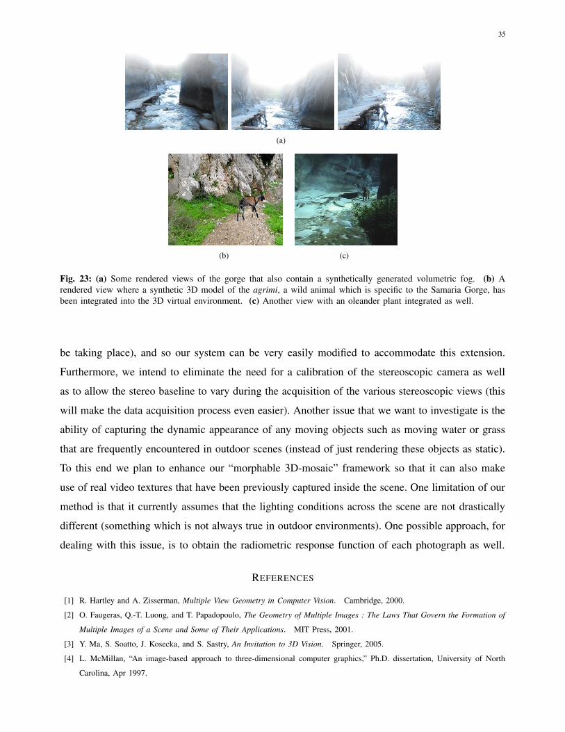
35

(a)

(b) (c)

Fig. 23: (a) Some rendered views of the gorge that also contain a synthetically generated volumetric fog. (b) Arendered view where a synthetic 3D model of the agrimi, a wild animal which is specific to the Samaria Gorge, hasbeen integrated into the 3D virtual environment. (c) Another view with an oleander plant integrated as well.

be taking place), and so our system can be very easily modified to accommodate this extension.

Furthermore, we intend to eliminate the need for a calibration of the stereoscopic camera as well

as to allow the stereo baseline to vary during the acquisition of the various stereoscopic views (this

will make the data acquisition process even easier). Another issue that we want to investigate is the

ability of capturing the dynamic appearance of any moving objects such as moving water or grass

that are frequently encountered in outdoor scenes (instead of just rendering these objects as static).

To this end we plan to enhance our “morphable 3D-mosaic” framework so that it can also make

use of real video textures that have been previously captured inside the scene. One limitation of our

method is that it currently assumes that the lighting conditions across the scene are not drastically

different (something which is not always true in outdoor environments). One possible approach, for

dealing with this issue, is to obtain the radiometric response function of each photograph as well.

REFERENCES

[1] R. Hartley and A. Zisserman, Multiple View Geometry in Computer Vision. Cambridge, 2000.

[2] O. Faugeras, Q.-T. Luong, and T. Papadopoulo, The Geometry of Multiple Images : The Laws That Govern the Formation of

Multiple Images of a Scene and Some of Their Applications. MIT Press, 2001.

[3] Y. Ma, S. Soatto, J. Kosecka, and S. Sastry, An Invitation to 3D Vision. Springer, 2005.

[4] L. McMillan, “An image-based approach to three-dimensional computer graphics,” Ph.D. dissertation, University of North

Carolina, Apr 1997.

36

[5] E. H. Adelson and J. R. Bergen, “The plenoptic function and the elements of early vision,” in Computational Models of Visual

Processing. Cambridge, MA: MIT Press, 1991, pp. 3–20.

[6] N. Komodakis, G. Pagonis, and G. Tziritas, “Interactive walkthroughs using morphable 3d-mosaics,” in Proc.of the second

International Symposium on 3DPVT (3DPVT 2004), 2004.

[7] N. Komodakis and G. Tziritas, “Morphable 3d-mosaics: a framework for the visual reconstruction of large natural scenes,” to

appear in the video proceedings of CVPR 2006.

[8] S. Teller, “Automated urban model acquisition: Project rationale and status,” in Teller, S. (1998). Automated urban model

acquisition: Project rationale and status. In Proceedings of the Image Understanding Workshop (pp. 455–462). Monterey, CA.,

1998.

[9] H.-Y. Shum, R. Szeliski, S. Baker, M. Han, and P. Anandan, “Interactive 3d modeling from multiple images using scene

regularities.” in SMILE, 1998, pp. 236–252.

[10] D. Nister, “Automatic passive recovery of 3d from images and video.” in 3DPVT, 2004, pp. 438–445.

[11] R. Koch, “3d surface reconstruction from stereoscopic image sequences,” in Proc. of the IEEE Int. Conf. on Computer Vision

(ICCV 1995), 1995, pp. 109–114.

[12] M. Pollefeys, L. J. V. Gool, M. Vergauwen, F. Verbiest, K. Cornelis, J. Tops, and R. Koch, “Visual modeling with a hand-held

camera.” International Journal of Computer Vision, vol. 59, no. 3, pp. 207–232, 2004.

[13] C. Strecha, R. Fransens, and L. J. V. Gool, “Wide-baseline stereo from multiple views: A probabilistic account.” in CVPR (1),

2004, pp. 552–559.

[14] C. Strecha and L. J. V. Gool, “Pde-based multi-view depth estimation.” in 3DPVT, 2002, pp. 416–427.

[15] C. Strecha, T. Tuytelaars, and L. J. V. Gool, “Dense matching of multiple wide-baseline views.” in ICCV, 2003, pp. 1194–1201.

[16] P. E. Debevec, C. J. Taylor, and J. Malik, “Modeling and rendering architecture from photographs: A hybrid geometry- and

image-based approach,” in SIGGRAPH 96, 1996, pp. 11–20.

[17] S. Fleishman, B. Chen, A. Kaufman, and D. Cohen-Or, “Navigating through sparse views,” in VRST99, pp. 82-87, 1999.

[18] L. McMillan and G. Bishop, “Plenoptic modeling: An image-based rendering approach,” in SIGGRAPH95, pp. 39-46, 1995.

[19] M. Levoy and P. Hanrahan, “Light field rendering,” in SIGGRAPH 96, 1996, pp. 31–42.

[20] S. Gortler, R. Grzeszczuk, R. Szeliski, and M. Cohen, “The lumigraph,” in SIGGRAPH 96, 1996, pp. 43–54.

[21] C. Buehler, M. Bosse, L. McMillan, S. J. Gortler, and M. F. Cohen, “Unstructured lumigraph rendering.” in Proc. of SIGGRAPH

2001, 2001, pp. 425–432.

[22] H. Schirmacher, M. Li, and H.-P. Seidel, “On-the-fly processing of generalized Lumigraphs,” in Proc. of Eurographics 2001,

vol. 20, no. 3, 2001, pp. C165–C173;C543.

[23] S. Vedula, S. Baker, and T. Kanade, “Spatio-temporal view interpolation,” in Proceedings of the 13th ACM Eurographics

Workshop on Rendering, June 2002.

[24] W. Matusik, C. Buehler, R. Raskar, S. J. Gortler, and L. McMillan, “Image-based visual hulls,” in Proc. of SIGGRAPH 2000,

2000, pp. 369–374.

[25] C. L. Zitnick, S. B. Kang, M. Uyttendaele, S. Winder, and R. Szeliski, “High-quality video view interpolation using a layered

representation,” ACM Trans. Graph., vol. 23, no. 3, pp. 600–608, 2004.

[26] M. Uyttendaele, A. Criminisi, S. B. Kang, S. Winder, R. Hartley, and R. Szeliski, “High-quality image-based interactive

exploration of real-world environments,” IEEE Computer Graphics & Applications, 2004.

[27] D. G. Aliaga, T. Funkhouser, D. Yanovsky, and I. Carlbom, “Sea of images,” in VIS 2002, 2002, pp. 331–338.

[28] J.-Y. Bouguet, “Camera Calibration Toolbox for MATLAB,” http://www.vision.caltech.edu/bouguetj/calib doc.

[29] I. Grinias and G. Tziritas, “Robust pan, tilt and zoom estimation.” in Intern. Conference on Digital Signal Processing, 2002.

37

[30] J. Barron, D. Fleet, and S. Beauchemin, “Performance of optical flow techniques,” International Journal of Computer Vision,

vol. 12, pp. 43–77, 1994.

[31] M. J. Black and P. Anandan, “The robust estimation of multiple motions: Parametric and piecewise-smooth flow fields,” CVIU,

vol. 63, no. 1, pp. 75–104, 1996.

[32] N. Komodakis and G. Tziritas, “A new framework for approximate labeling via graph-cuts.” in ICCV, 2005, pp. 1018–1025.

[33] S. Coorg and S. Teller, “Spherical mosaics with quaternions and dense correlation,” Int. J. Comput. Vision, vol. 37, no. 3, pp.

259–273, 2000.

[34] B. K. P. Horn, “Closed form solution of absolute orientation using unit quaternions,” Journal of The Optical Society of America

A, vol. 4, no. 4, April 1987.

[35] T. Tuytelaars and L. V. Gool, “Wide Baseline Stereo Matching based on Local, Affinely Invariant Regions,” in Proceedings

of British Machine Vision Conference, 2000, pp. 412–422.

[36] K. Mikolajczyk and C. Schmid, “An affine invariant interest point detector,” in ECCV (1), 2002, pp. 128–142.

[37] D. G. Lowe, “Distinctive image features from scale-invariant keypoints,” Int. J. Comput. Vision, vol. 60, no. 2, pp. 91–110,

2004.

[38] S. Li, Markov Random Field Modeling in Computer Vision. Springer-Verlag, 1995.

[39] P. F. Felzenszwalb and D. P. Huttenlocher, “Efficient belief propagation for early vision.” in CVPR, 2004, pp. 261–268.

[40] Y. Boykov, O. Veksler, and R. Zabih, “Fast approximate energy minimization via graph cuts,” IEEE Transactions on Pattern

Analysis and Machine Intelligence, vol. 23, no. 11, pp. 1222–1239, November 2001.

[41] D. Zwilliger, Handbook of Differential Equations. Boston, MA: Academic Press, 1997.

[42] P. Perez, M. Gangnet, and A. Blake, “Poisson image editing,” ACM Trans. Graph., vol. 22, no. 3, pp. 313–318, 2003.

[43] M. Segal and K. Akeley, “The OpenGL Graphics System: A Specification (Version 1.5),” http://www.opengl.org.

[44] P. S. Heckbert and M. Garland, “Survey of polygonal surface simplification algorithms,” in SIGGRAPH 97 course notes on

multiresolution surface modeling.

[45] R. Szeliski, “Video mosaics for virtual environments,” IEEE Computer Graphics and Applications, vol. 16, no. 2, pp. 22–30,

March 1996.