1 tutorial document of itm638 data warehousing and data mining dr. chutima beokhaimook 24 th march...
TRANSCRIPT

1
Tutorial Document ofITM638 Data Warehousing
and Data Mining
Dr. Chutima Beokhaimook
24th March 2012
DATA WAREHOUSES AND OLAP TECHNOLOGY
2

3
What is Data Warehouse?
Data warehouse have been defined in many ways “A data warehouse is a subject-oriented, integrated,
time-variant and non-volatile collection of data in support of management’s decision making process” – W.H. Inmon
The four keywords :- subject-oriented, integrated, time-variant and non-volatile
4
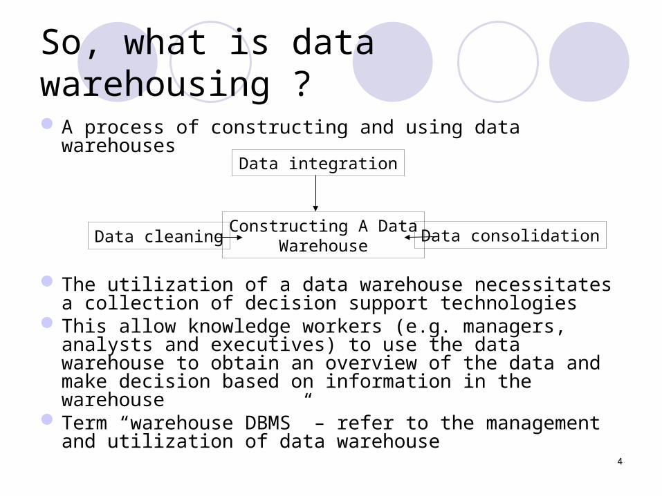
So, what is data warehousing ?
A process of constructing and using data warehouses
The utilization of a data warehouse necessitates a collection of decision support technologies
This allow knowledge workers (e.g. managers, analysts and executives) to use the data warehouse to obtain an overview of the data and make decision based on information in the warehouse
Term “warehouse DBMS” – refer to the management and utilization of data warehouse
Constructing A Data Warehouse
Data integration
Data cleaning Data consolidation

5
Operational Database vs. Data Warehouses
Operational DBMSOLTP (on-line transaction processing)
Day-to-day operations of an organization such as purchasing, inventory, manufacturing, banking, etc.
Data warehousesOLAP (on-line analytical processing)
Serve users or knowledge workers in the role of data analysis and decision making
The system can organize and present data in various formats

6
OLTP vs. OLAP
Feature OLTP OLAP
Characteristic Operational Processing Informational processing
users Clerk, IT professional Knowledge worker
Orientation transaction Analysis
Function Day-to-day operation Long-term informational requirements, DSS
DB design ER based, application-oriented
Star/snowflake, subject-oriented
Data Current, guaranteed up-to-date
Historical; accuracy maintained over time
Summarization Primitive, highly detailed Summarized, consolidated
# of record access Tens Millions
# of users Thousands Hundreds
DB size 100 MB to GB 100GB to TB

7
Why Have a Separate Data warehouse?
High performance for both systems An operational database – tuned for OLTP: access methods,
indexing, concurrency control, recovery A data warehouse – tuned for OLAP: complex OLAP queries,
multidimensional view, consolidation
Different functions and different data DSS require historical data, whereas operational DB do not
maintain historical data DSS require consolidation (such as aggregation and
summarization) of data from heterogeneous sources, resulting in high-quality, clean, and integrated data, whereas operational DB contain only detailed raw data, which need to be consolidate before analysis
8
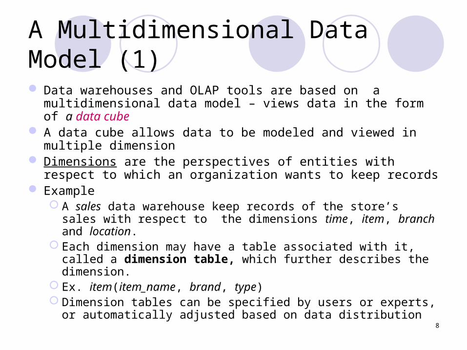
A Multidimensional Data Model (1)
Data warehouses and OLAP tools are based on a multidimensional data model – views data in the form of a data cube
A data cube allows data to be modeled and viewed in multiple dimension
Dimensions are the perspectives of entities with respect to which an organization wants to keep records
Example A sales data warehouse keep records of the store’s sales with
respect to the dimensions time, item, branch and location. Each dimension may have a table associated with it, called a
dimension table, which further describes the dimension. Ex. item(item_name, brand, type) Dimension tables can be specified by users or experts, or
automatically adjusted based on data distribution

9
A Multidimensional Data Model (2)
A multidimensional model is organized around a central theme, for instance, sales, which is represented by a fact table
Facts are numerical measures such as quantities :-dolar_sold, unit_sold, amount_budget
10
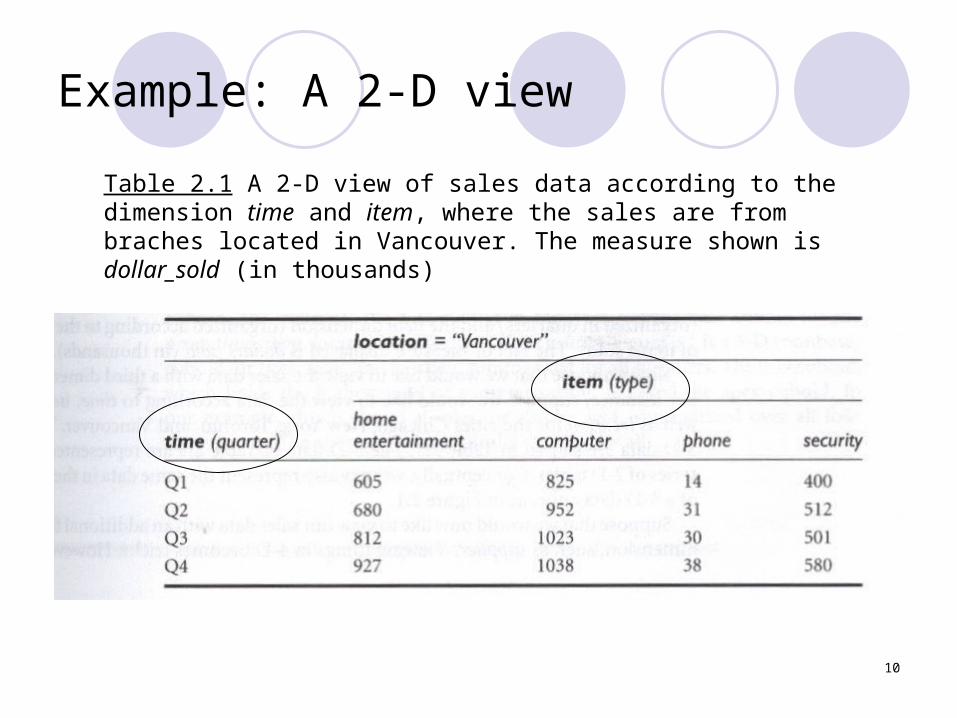
Example: A 2-D view
Table 2.1 A 2-D view of sales data according to the dimension time and item, where the sales are from braches located in Vancouver. The measure shown is dollar_sold (in thousands)

11
Example: A 3-D View
Table 2.2 A 3-D view of sales data according to the dimension time and item and location. The measure shown is dollar_sold (in thousands)

12
Example: A 3-D data cube
A 3-D data cube represent the data in table 2.2 according to the dimension time and item and location. The measure shown is dollar_sold (in thousands)

13
Star Schema
The most common modeling paradigm, in which the data warehouse contains
1. A large central table (fact table) containing the bulk of the data, no redundancy
2. A set of smaller attendant table (dimension table), one for each dimension
14
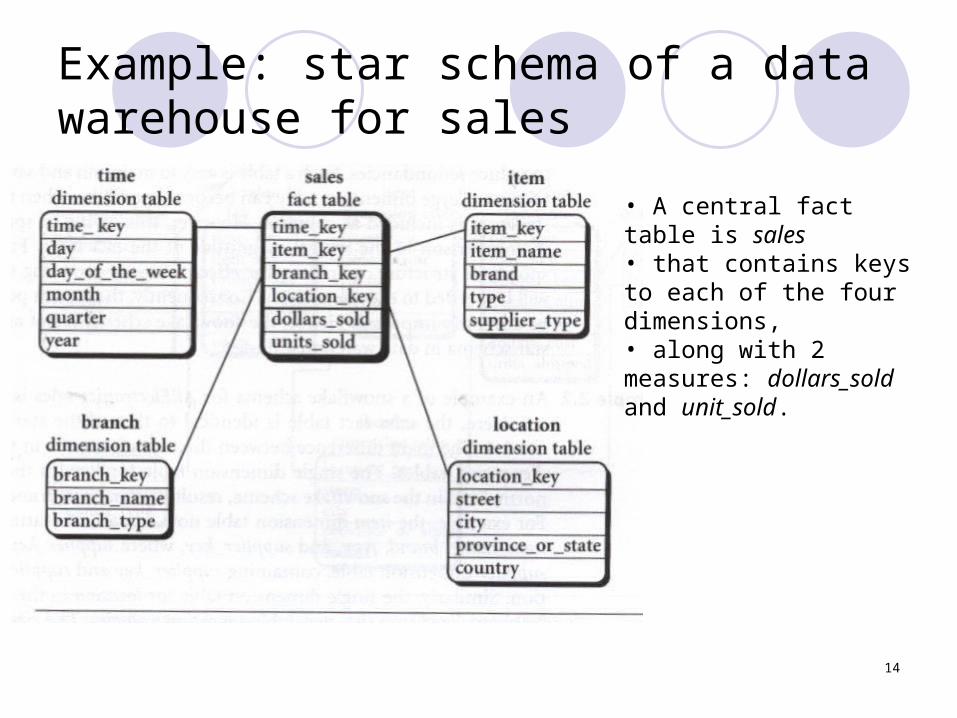
Example: star schema of a data warehouse for sales
• A central fact table is sales• that contains keys to each of the four dimensions,• along with 2 measures: dollars_sold and unit_sold.

15
Example: snowflake schema of a data warehouse for sales

16
Example: fact constellation schema of a data warehouse for sales and shipping
2 fact models
17
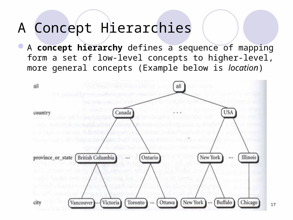
A Concept HierarchiesA concept hierarchy defines a sequence of mapping
form a set of low-level concepts to higher-level, more general concepts (Example below is location)
18
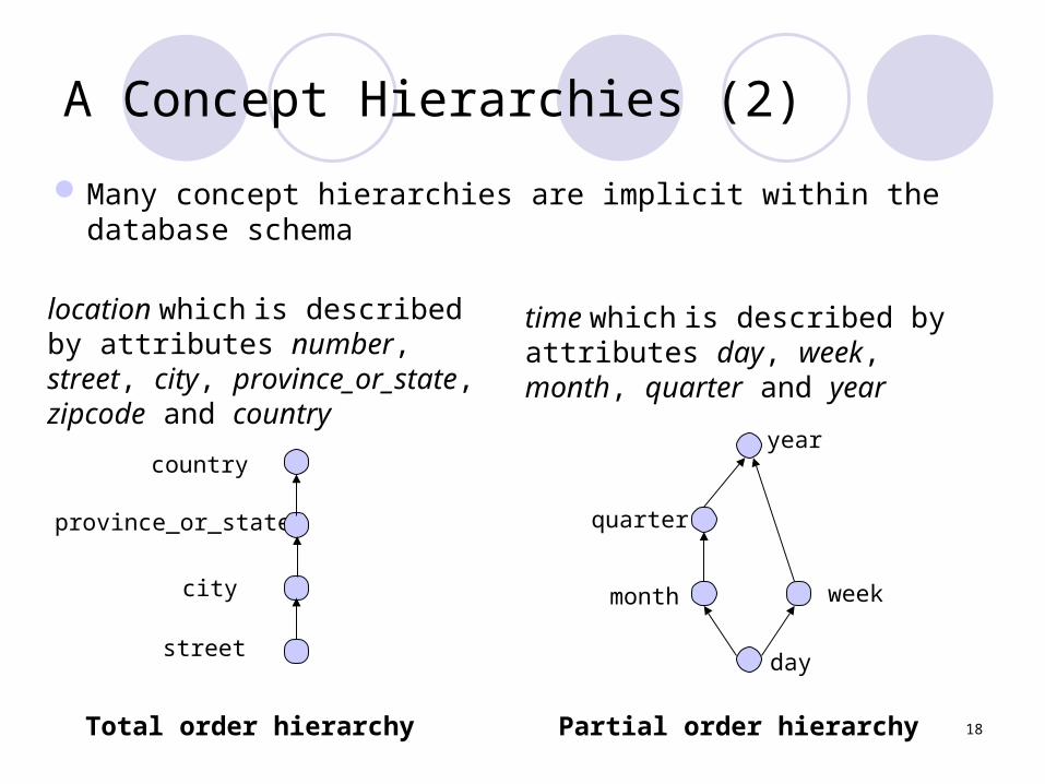
A Concept Hierarchies (2)
Many concept hierarchies are implicit within the database schema
street
city
province_or_state
country
location which is described by attributes number, street, city, province_or_state, zipcode and country
Total order hierarchy
day
month
quarter
year
week
time which is described by attributes day, week, month, quarter and year
Partial order hierarchy

19
Typical OLAP Operations for multidimensional data (1)
Roll-up (drill-up): climbing up a concept hierarchy or dimension reduction – summarize data
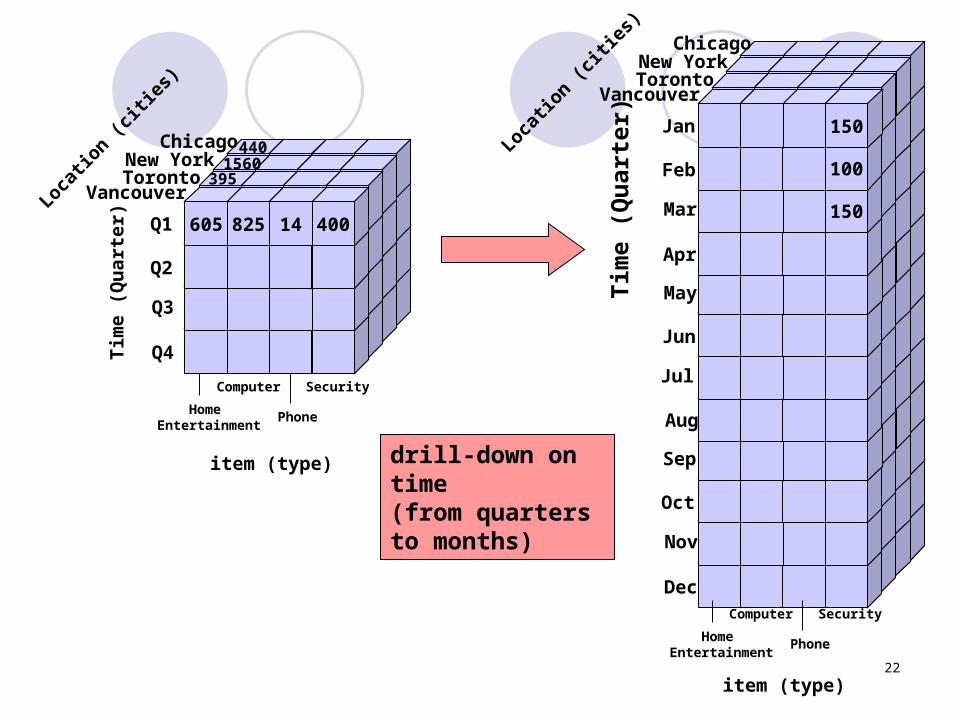
Drill down(roll-down): stepping down a concept hierarchy or introducing additional dimensions reverse of roll-up Navigate from less detailed data to more detailed data
Slice and dice: Slice operation perform a selection on one dimension of the
given cube, resulting in subcube. Dice operation defines a subcube by performing a selection on
two or more dimensions

20
Typical OLAP Operations for multidimensional data (2)
Pivot (rotate): A visualization operation that rotate data axes in view in order to
provide an alternative presentation of the data
Other OLAP operations: such as drill-across – execute queries involving more than one fact table drill-through
21
605 825 14 400Q1
Q2
Q3
Q4
Tim
e (Q
uar
ter)
Locatio
n (citi
es)
3951560
440
VancouverTorontoNew York
Chicago
Home Entertainment
Computer
Phone
Security
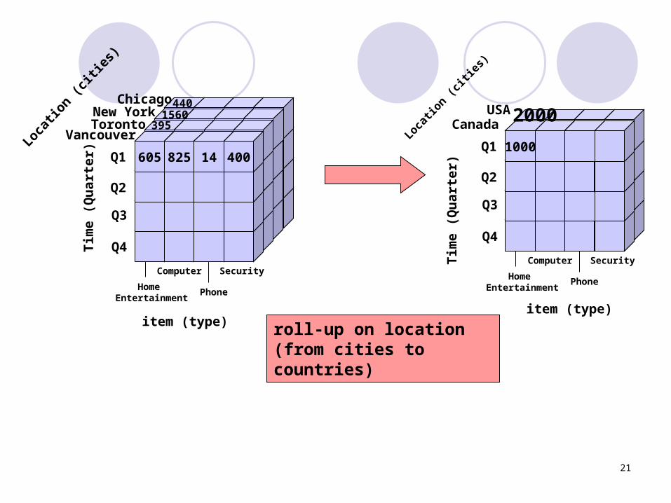
item (type) roll-up on location (from cities to countries)
1000Q1
Q2
Q3
Q4
Tim
e (Q
uar
ter)
Locatio
n (citi
es)
2000Canada
USA
Home Entertainment
Computer
Phone
Security
item (type)
22
Sep
Oct
Nov
Dec
Aug
May
Jun
Jul
605 825 14 400Q1
Q2
Q3
Q4
Tim
e (Q
uar
ter)
Locatio
n (citi
es)
3951560
440
VancouverTorontoNew York
Chicago
Home Entertainment
Computer
Phone
Security
item (type) drill-down on time (from quarters to months)
150
100
150Jan
Feb
Mar
Apr
Tim
e (Q
uar
ter)
VancouverTorontoNew York
Chicago
Home Entertainment
Computer
Phone
Security
item (type)
Locatio
n (citi
es)

23
605 825 14 400605
Q1
Q2
Q3
Q4Tim
e (Q
uar
ter)
Locatio
n (citi
es)
3951560
440
VancouverTorontoNew York
Chicago
Home Entertainment
Computer
Phone
Security
item (type)
395VancouverToronto
Home Entertainment
Computer
Q1
Q2
dice for (location=“Toronto”or“Vancouver”)and (time = “Q1” or “Q2”) and (item=“home entertainment” or “computer”)
item (type)
Locatio
n (citi
es)

24
605 825 14 400Q1
Q2
Q3
Q4
Tim
e (Q
uar
ter)
Locatio
n (citi
es)
3951560
440
VancouverTorontoNew York
Chicago
Home Entertainment
Computer
Phone
Security
item (type)
slice for (time=“Q1”)
825 14605 400
Chicago
New York
Toronto
Vancouver
Home Entertainment
Computer
Phone
Security
item (type)1560 395440 605
825
14
400
Chicago
New York
Toronto
Home Entertainment
Computer
Phone
Securityitem
(ty
pe)
Vancouver
pivot
Location (cities)
MINING FREQUENT PATTERN, ASSOCIATIONS
25

26
What is Association Mining?
Association rule mining:Finding frequent patterns, associations, correlations, or
causal structures among sets of items or objects in transaction databases, relational databases, and other information repositories
Applications:Basket data analysis, cross-marketing, catalog design,
loss-leader analysis, clustering, classification, etc.Rule form: “Body Head [support, confidence]”
buys(x, “diapers”) buys(x, “beers”) [0.5%,60%]major(x, “CS”) take (x, “DB”) grade (x, “A”) [1%,75%]
27
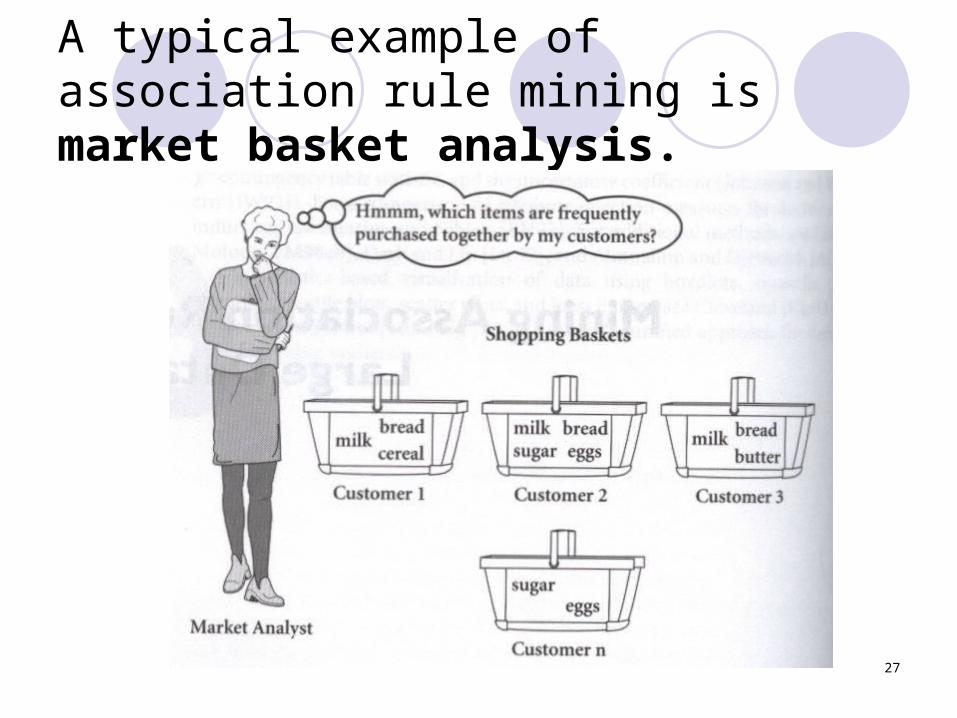
A typical example of association rule mining is market basket analysis.

28
The information that customers who purchase computer also tend to buy antivirus software at the same time is represented in Association Rule below:computer antivirus_software
[support = 2%, confidence = 60%]Rule support and confidence are two measures of rule
interestingness Support= 2% means that 2% of all transactions under analysis
show that computer and antivirus software are purchased together
Confidence=60% means that 60% of the customers who purchased a computer also bought the software
Typically, association rules are considered interesting if they satisfy both a minimum support threshold and a minimum confidence threshold
Such threshold can be set by users of domain experts

29
Rule Measure: Support and Confidence
Support: probability that a transaction contain {ABC}Confidence: Condition probability that a transaction having {AB} also contain {C}
TransID Items Bought
T001 A,B,C
T002 A,C
T003 A,D
T004 B,E,F
•Find all the rule A B C with minimum confidence and support•Let min_sup=50%, min_conf.=50%
Typically association rules are considered interesting if they satisfy both a minimum support threshold and a mininum confidence threshold
Such thresholds can be set by users or domain experts

30
Rules that satisfy both a minimum support threshold (min_sup) and a minimum confidence threshold (min_conf) are called strong
A set of items is referred to as an itemsetAn itemset that contains k items is a k-itemsetThe occurrence frequency of an itemset is the
number of transactions that contain the itemsetAn itemset satisfies minimum support if the occurrence
frequency of the itemset >= min_sup * total no. of transaction
An itemset satisfies minimum support it is a frequent itemset
31
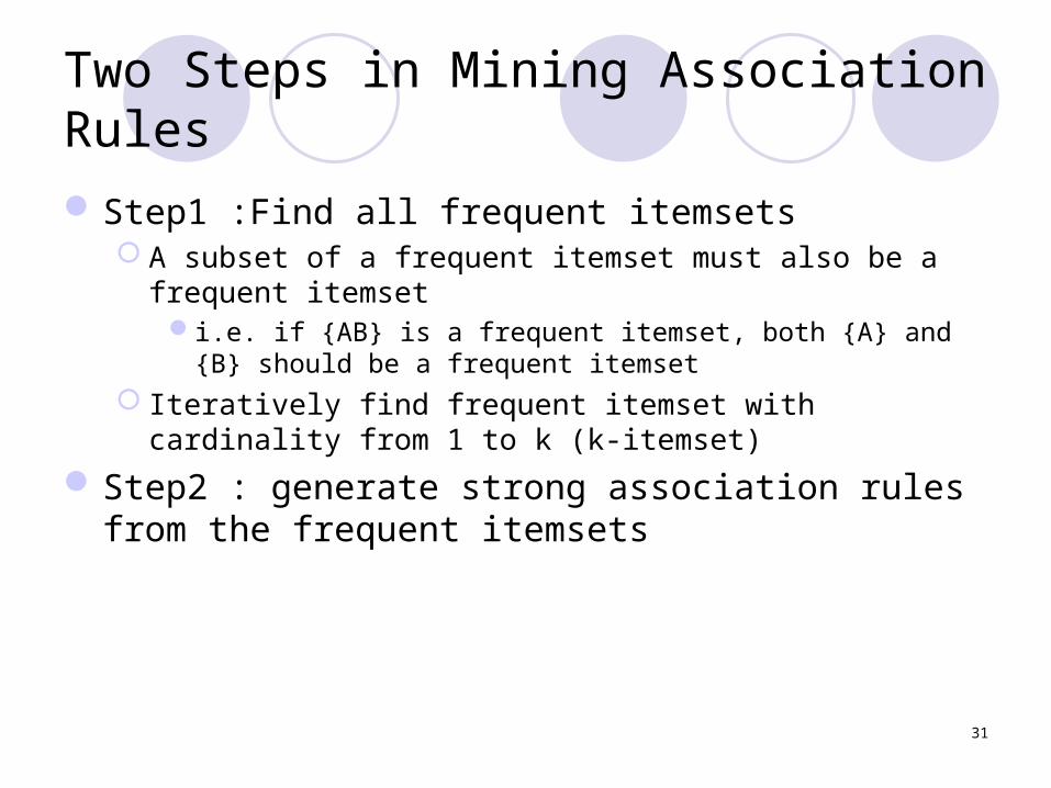
Two Steps in Mining Association Rules
Step1 :Find all frequent itemsets A subset of a frequent itemset must also be a frequent itemset
i.e. if {AB} is a frequent itemset, both {A} and {B} should be a frequent itemset
Iteratively find frequent itemset with cardinality from 1 to k (k-itemset)
Step2 : generate strong association rules from the frequent itemsets
32
Mining Single-Dimensional Boolean Association Rules From Transaction Databases
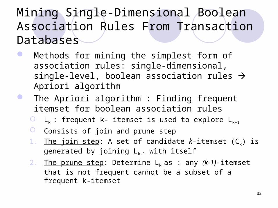
Methods for mining the simplest form of association rules: single-dimensional, single-level, boolean association rules Apriori algorithm
The Apriori algorithm : Finding frequent itemset for boolean association rules
Lk : frequent k- itemset is used to explore Lk+1
Consists of join and prune step
1. The join step: A set of candidate k-itemset (Ck) is generated by joining Lk-1 with itself
2. The prune step: Determine Lk as : any (k-1)-itemset that is not frequent cannot be a subset of a frequent k-itemset
33
The Apriori Algorithm
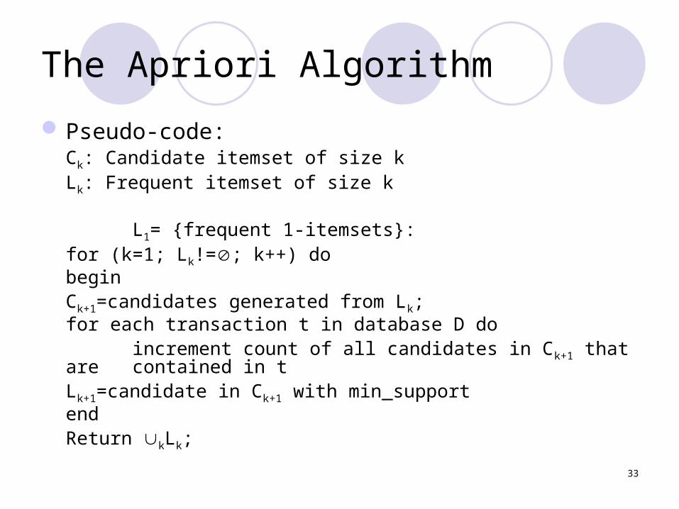
Pseudo-code: Ck: Candidate itemset of size k
Lk: Frequent itemset of size k L1= {frequent 1-itemsets}:
for (k=1; Lk!=; k++) dobegin
Ck+1=candidates generated from Lk;for each transaction t in database D do
increment count of all candidates in Ck+1 that are contained in t
Lk+1=candidate in Ck+1 with min_support end Return kLk;
34
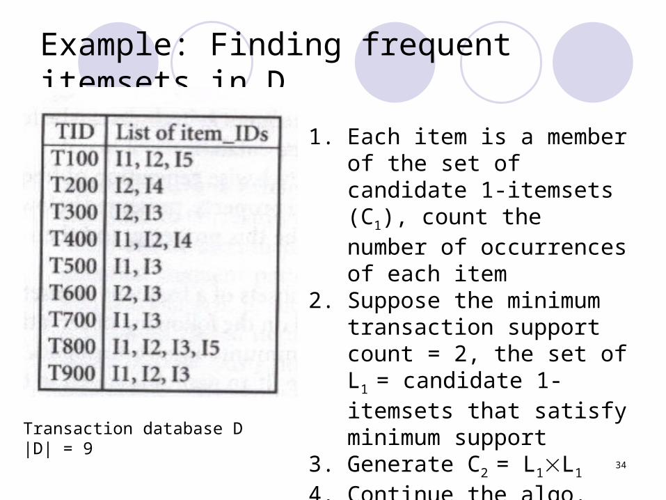
Example: Finding frequent itemsets in D
1. Each item is a member of the set of candidate 1-itemsets (C1), count the number of occurrences of each item
2. Suppose the minimum transaction support count = 2, the set of L1 = candidate 1-itemsets that satisfy minimum support
3. Generate C2 = L1L1
4. Continue the algo. Until C4=
Transaction database D|D| = 9

35
36
Example of Generating Candidates
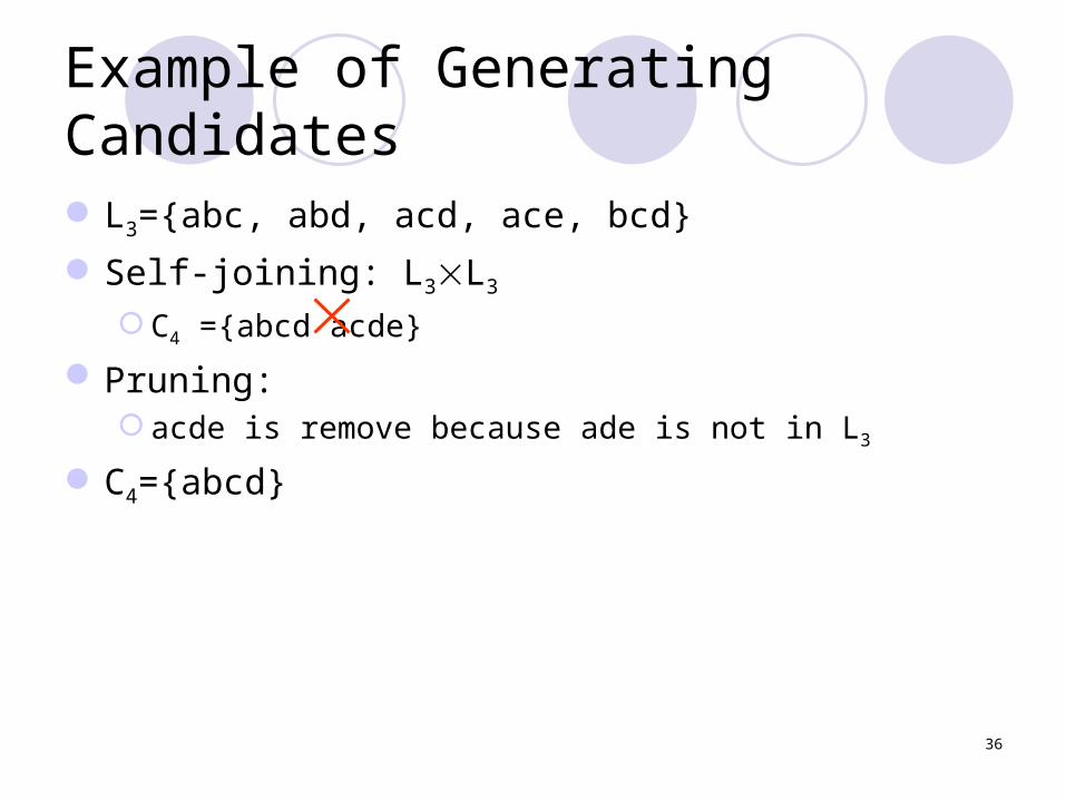
L3={abc, abd, acd, ace, bcd}
Self-joining: L3L3
C4 ={abcd acde}
Pruning: acde is remove because ade is not in L3
C4={abcd}
37
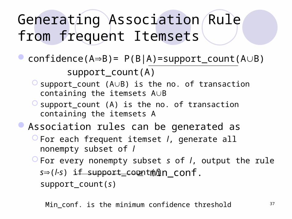
Generating Association Rule from frequent Itemsets
confidence(AB)= P(B|A)=support_count(AB)
support_count(A) support_count (AB) is the no. of transaction containing the
itemsets AB support_count (A) is the no. of transaction containing the
itemsets A
Association rules can be generated as For each frequent itemset l, generate all nonempty subset of l For every nonempty subset s of l, output the rule
s(l-s) if support_count(l)
support_count(s)
Min_conf. is the minimum confidence threshold
min_conf.

38
Example
Suppose the data contain the frequent itemset l={I1,I2,I5}What are the association rules that can be generated from l?
The nonempty subsets of l are {I1,I2}, {I1,I5}, {I2,I5}, {I1}, {I2}, {I5} The resulting association rules are
1 l1l2l5 confidence=2/4=50%
2 l1l5l2 confidence=2/2=100%
3 l2l5l1 confidence=2/2=100%
4 l1l2l5 confidence=2/6=33%
5 l2l1l5 confidence=2/7=29%
6 l5l1l2 confidence=2/2=100% If minimun confidence threshold = 70% Output are the rule no. 2,3 and 6
CLASSIFICATION AND PREDICTION
39

40
Lecture 5 Classification and Prediction
Chutima PisarnFaculty of Technology and Environment
Prince of Songkla University
976-451 Data Warehousing and Data Mining
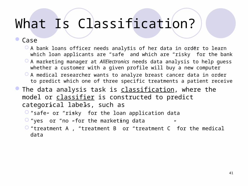
What Is Classification?Case
A bank loans officer needs analysis of her data in order to learn which loan applicants are “safe” and which are “risky” for the bank
A marketing manager at AllElectronics needs data analysis to help guess whether a customer with a given profile will buy a new computer
A medical researcher wants to analyze breast cancer data in order to predict which one of three specific treatments a patient receive
The data analysis task is classification, where the model or classifier is constructed to predict categorical labels, such as “safe” or “risky” for the loan application data “yes” or “no” for the marketing data “treatment A”, “treatment B” or “treatment C” for the medical data
41

What Is Prediction?
Suppose that the marketing manager would like to predict how much a given customer will spend during a sale at AllElectronics
This data analysis task is numeric prediction, where the model constructed predicts a continuous value or ordered values, as opposed to a categorical label
This model is a predictorRegression analysis is a statistical methodology that
is most often used for numeric prediction
42

43
How does classification work?
Data classification is a two-step process In the first step, -- learning step or training phase
a model is built describing a predetermined set of data classes or concepts
The model is constructed by analyzing database tuples described by attributes
Each tuple is assumed to belong to a predefined class, as determined by the class label attribute
Data tuples used to build the model are called training data set The individual tuples in a training set are referred to as training
samples If the class label is provided, this step is known as supervised
learning, otherwise called unsupervised learning (or clustering) The learned model is represented in the form of classification
rules, decision trees or mathematical formulae
44
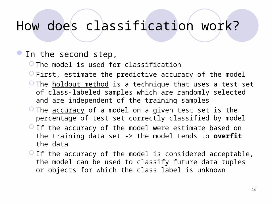
How does classification work?
In the second step, The model is used for classification First, estimate the predictive accuracy of the model The holdout method is a technique that uses a test set of class-
labeled samples which are randomly selected and are independent of the training samples
The accuracy of a model on a given test set is the percentage of test set correctly classified by model
If the accuracy of the model were estimate based on the training data set -> the model tends to overfit the data
If the accuracy of the model is considered acceptable, the model can be used to classify future data tuples or objects for which the class label is unknown

45
How is prediction different from classification?
Data prediction is a two step process, similar to that of data classification
For prediction, the attributefor which values are being predicted is continuous-value (ordered) rather than categorical (discrete-value and unordered)
Prediction can also be viewed as a mapping or function, y=f(X)

46
Classification by Decision Tree Induction
A decision tree is a flow-chart-like tree structure, each internal node denotes a test on an attribute, each branch represents an outcome of the test leaf node represent classes Top-most node in a tree is the root node
Age?
student? Credit_rating?
no yes
yes
yesno
<=3031…40
>40
no yes excellent fair
The decision tree represents the concept buys_computer

47
Attribute Selection Measure
The information gain measure is used to select the test attribute at each node in the tree
Information gain measure is referred to as an attribute selection measure or measure of the goodness of split
The attribute with the highest information gain is chosen as the test attribute for the current node
Let S be a set consisting of s data samples, the class label attribute has m distinct value defining m distinct classes, Ci (for i=1,...,m)
Let si be the no of sample of S in class Ci
The expected information I(s1,s2,…sm)=- pi log2(pi),
where pi is the probability that the sample belongs to class, pi =si/si=1
m
48
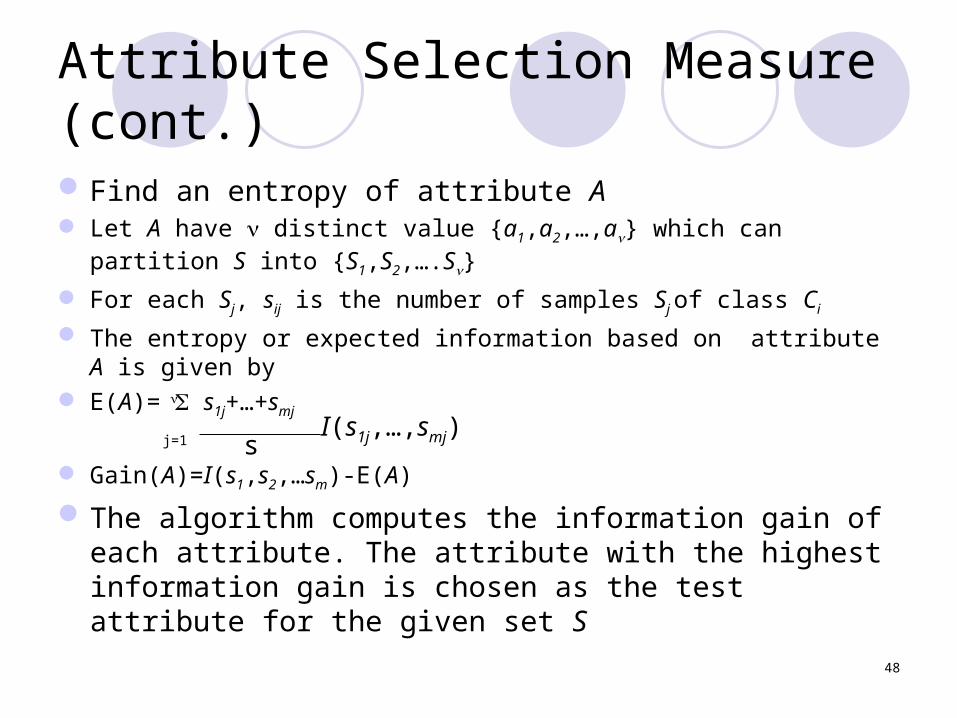
Attribute Selection Measure (cont.)
Find an entropy of attribute A Let A have distinct value {a1,a2,…,a} which can partition S into
{S1,S2,….S}
For each Sj, sij is the number of samples Sj of class Ci
The entropy or expected information based on attribute A is given by
E(A)= s1j+…+smj
Gain(A)=I(s1,s2,…sm)-E(A)
The algorithm computes the information gain of each attribute. The attribute with the highest information gain is chosen as the test attribute for the given set S
sI(s1j,…,smj)j=1

49
ExampleRID age income studen
tCredit_rating
Class:buys_computer
1 <=30 High No Fair No
2 <=30 High No Excellent No
3 31…40 High No Fair Yes
4 >40 Medium No Fair Yes
5 >40 Low Yes Fair Yes
6 >40 Low Yes Excellent No
7 31…40 Low Yes Excellent Yes
8 <=30 Medium No Fair no
9 <=30 Low Yes Fair Yes
10 >40 Medium Yes Fair Yes
11 <=30 Medium Yes Excellent Yes
12 31…40 Medium No Excellent Yes
13 31…40 High Yes Fair Yes
14 >40 medium no Excellent No
the class label attribute: 2 classes
I(s1,s2) = I(9,5) =-9/14 log2 (9/14)-5/14log2(5/14)=0.940
50
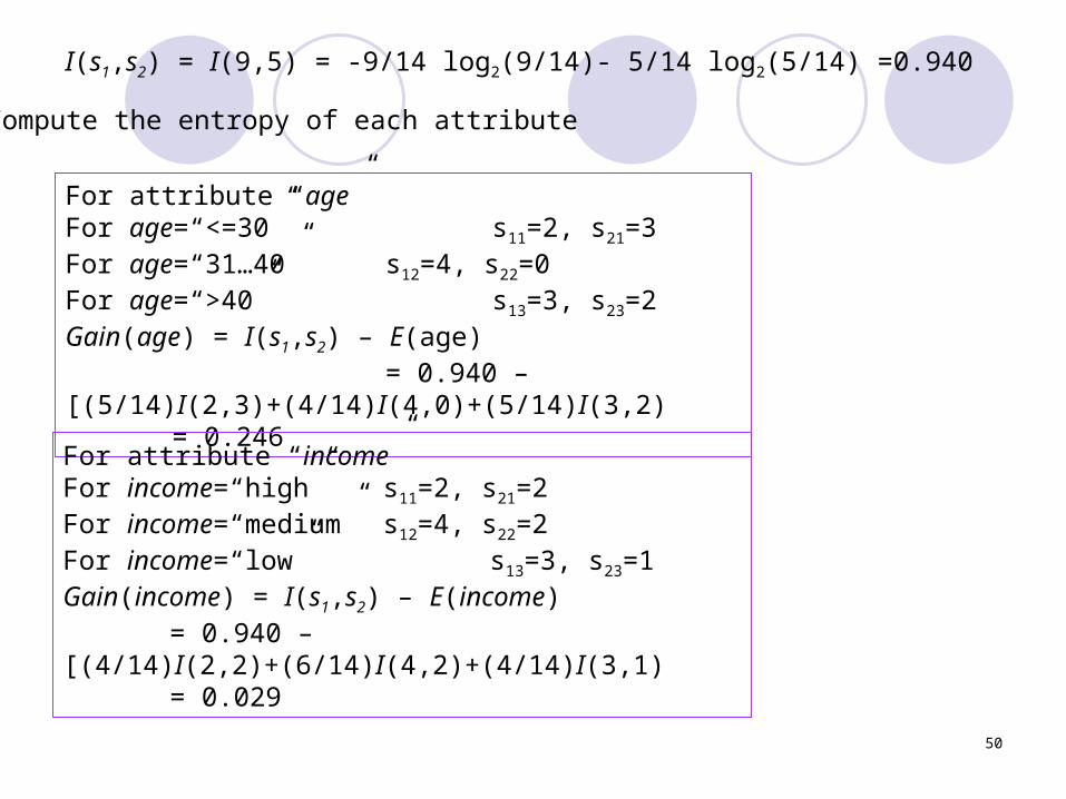
I(s1,s2) = I(9,5) = -9/14 log2(9/14)- 5/14 log2(5/14) =0.940
Compute the entropy of each attribute
For attribute “age” For age=“<=30” s11=2, s21=3For age=“31…40” s12=4, s22=0For age=“>40” s13=3, s23=2Gain(age) = I(s1,s2) – E(age) = 0.940 –[(5/14)I(2,3)+(4/14)I(4,0)+(5/14)I(3,2)
= 0.246
For attribute “income” For income=“high” s11=2, s21=2For income=“medium” s12=4, s22=2For income=“low” s13=3, s23=1Gain(income) = I(s1,s2) – E(income)
= 0.940 –[(4/14)I(2,2)+(6/14)I(4,2)+(4/14)I(3,1)= 0.029
51
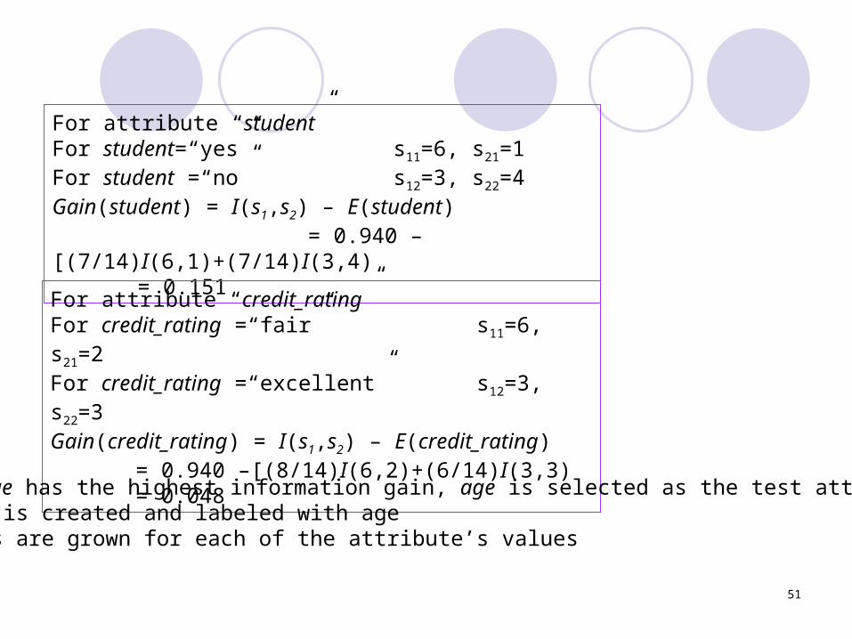
For attribute “student” For student=“yes” s11=6, s21=1For student =“no” s12=3, s22=4Gain(student) = I(s1,s2) – E(student) = 0.940 –[(7/14)I(6,1)+(7/14)I(3,4)
= 0.151
For attribute “credit_rating” For credit_rating =“fair” s11=6, s21=2For credit_rating =“excellent” s12=3, s22=3Gain(credit_rating) = I(s1,s2) – E(credit_rating)
= 0.940 –[(8/14)I(6,2)+(6/14)I(3,3)= 0.048
Since age has the highest information gain, age is selected as the test attribute-A node is created and labeled with age-Braches are grown for each of the attribute’s values
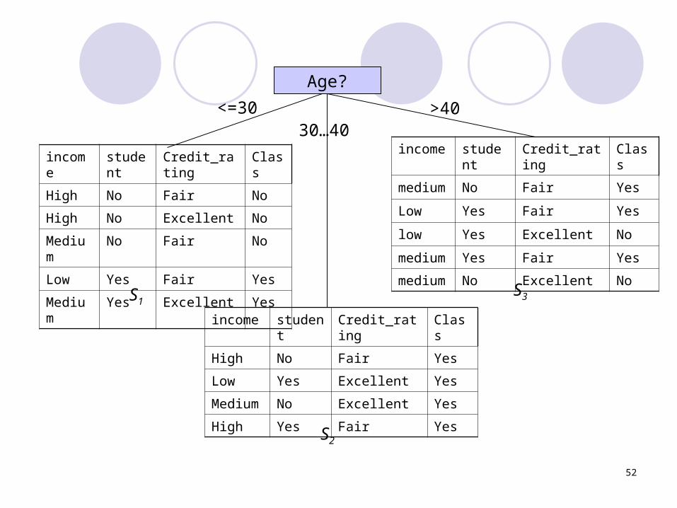
52
income student
Credit_rating
Class
High No Fair No
High No Excellent No
Medium No Fair No
Low Yes Fair Yes
Medium Yes Excellent Yes
income student Credit_rating Class
medium No Fair Yes
Low Yes Fair Yes
low Yes Excellent No
medium Yes Fair Yes
medium No Excellent No
Age?
<=3030…40
>40
income student Credit_rating Class
High No Fair Yes
Low Yes Excellent Yes
Medium No Excellent Yes
High Yes Fair Yes
S1S3
S2
53
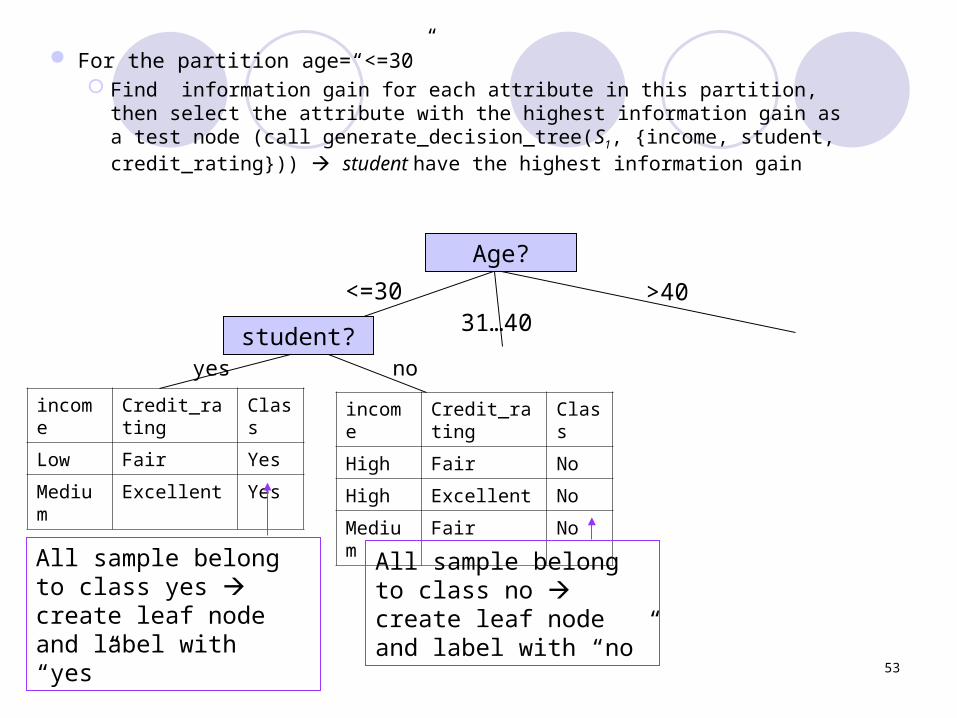
For the partition age=“<=30” Find information gain for each attribute in this partition, then
select the attribute with the highest information gain as a test node (call generate_decision_tree(S1, {income, student, credit_rating})) student have the highest information gain
income Credit_rating
Class
Low Fair Yes
Medium Excellent Yes
Age?
<=3031…40
>40
student?
income Credit_rating
Class
High Fair No
High Excellent No
Medium Fair No
yes no
All sample belong to class yes create leaf node and label with “yes”
All sample belong to class no create leaf node and label with “no”

54
Age?
student?
no yes
yes
<=3031…40
>40
no yesincome student Credit_rating Class
medium No Fair Yes
Low Yes Fair Yes
low Yes Excellent No
medium Yes Fair Yes
medium No Excellent No
For the partition age=“30…40” All sample belong to class no create leaf node and label with “no”
For the partition age=“>40” Consider credit rating and income credit rating has higher
information gain

55
Age?
student?
no yes
yes
<=3031…40
>40
no yes
Attribute left is income but sample is empty terminate generate_decision_tree
yesno
excellent fair
Credit_rate?
Assignment 1 แสดงการสร�าง Decision Tree นี้�� อย่�างละเอ�ย่ด แสดงการคำ�านี้วณด�วย่
56
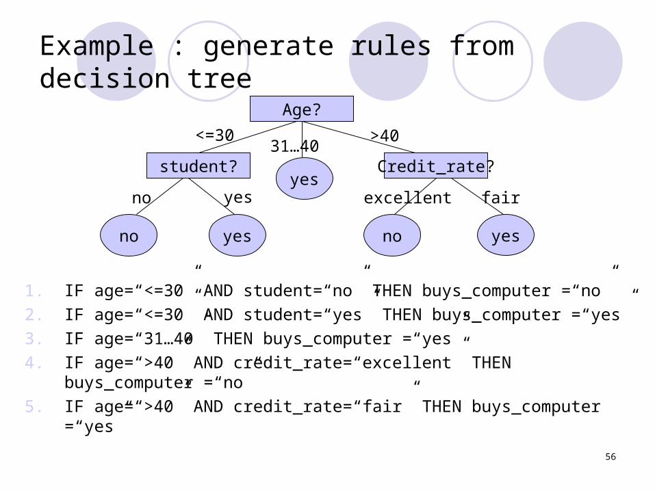
Example : generate rules from decision tree
1. IF age=“<=30” AND student=“no” THEN buys_computer =“no”
2. IF age=“<=30” AND student=“yes” THEN buys_computer =“yes”
3. IF age=“31…40” THEN buys_computer =“yes”
4. IF age=“>40” AND credit_rate=“excellent” THEN buys_computer =“no”
5. IF age=“>40” AND credit_rate=“fair” THEN buys_computer =“yes”
Age?
student?
no yes
yes
<=3031…40
>40
no yes
yesno
excellent fair
Credit_rate?
57
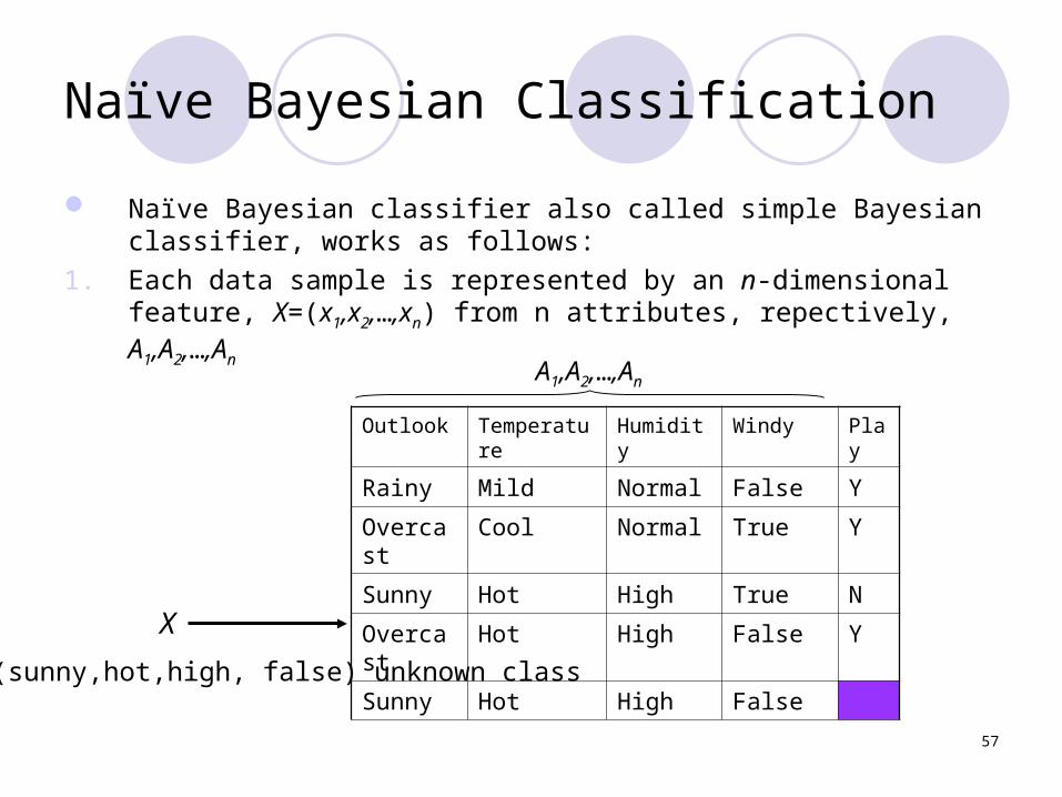
Naïve Bayesian Classification
Naïve Bayesian classifier also called simple Bayesian classifier, works as follows:
1. Each data sample is represented by an n-dimensional feature, X=(x1,x2,…,xn) from n attributes, repectively, A1,A2,…,An
Outlook Temperature
Humidity Windy Play
Rainy Mild Normal False Y
Overcast Cool Normal True Y
Sunny Hot High True N
Overcast Hot High False Y
Sunny Hot High FalseX
X=(sunny,hot,high, false) unknown class
A1,A2,…,An

58
Naïve Bayesian Classification (cont.)
2. Suppose that there are m clases, C1,C2,…Cm
Given an unknown data sample X The calssifier will predict that X belongs to the class having the
highest posterior probability, condition on X The naïve Bayesian will assigns an unknown X to class Ci if
and only if
P(Ci|X) > P(Cj|X) for 1 j m, jI
That is, it will find the maximum posterior probability among P(C1|X), P(C2|X), ….,P(Cm|X)
The class Ci for which P(Ci|X) is maximized is called the maximum posteriori hypothesis

59
Outlook Temperature
Humidity Windy Play
Rainy Mild Normal False Y
Overcast Cool Normal True Y
Sunny Hot High True N
Overcast Hot High False Y
Sunny Hot High FalseX
X=(sunny,hot,high,false) unknown class
A1,A2,…,An
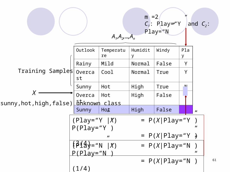
m =2C1: Play=“Y” and C2: Play=“N”
If (Play=“Y” | X) > (Play=‘N’| X)
Y
Training Samples

60
Naïve Bayesian Classification (cont.)
3. By Bayes theorem, P(Ci|X) = P(X|Ci) P(Ci)
P(X) As P(X) is constant for all classes, only P(X|Ci) P(Ci) need to
be maximized If P(Ci) are not known, it is commonly assume that P(C1) =
P(C2) = … = P(Cm), therefore only P(X|Ci) need to be maximized
Otherwise, we maximize P(X|Ci) P(Ci) ,
where P(Ci) = si
s# of training sample of Class Ci
Total # of training sample
61
Outlook Temperature
Humidity Windy Play
Rainy Mild Normal False Y
Overcast Cool Normal True Y
Sunny Hot High True N
Overcast Hot High False Y
Sunny Hot High FalseX
X=(sunny,hot,high,false) unknown class
A1,A2,…,An
m =2C1: Play=“Y” and C2: Play=“N”
(Play=“Y”|X) = P(X|Play=“Y”) P(Play=“Y”) = P(X|Play=“Y”) (3/4)
Training Samples
(Play=“N”|X) = P(X|Play=“N”) P(Play=“N”) = P(X|Play=“N”) (1/4)

62
Naïve Bayesian Classification (cont.)
4. Given a data sets with many attribute it is expensive to compute P(X|Ci)
To reduce computation, naïve made an assumption of class conditional independence (there are no dependence relationship among the attribute)
P(X|Ci) = P(xk|Ci) = P(x1|Ci)* P(x2|Ci)*…* P(xk|Ci)
If Ak is categorical, then P(xk|Ci) = sik
If Ak is continuous values perform Gaussian distribution (not focus in this class)
k=1
n
si
# of training sample of Class Ci having the value xk for Ak
Total # of training sample belong to class Ci
63
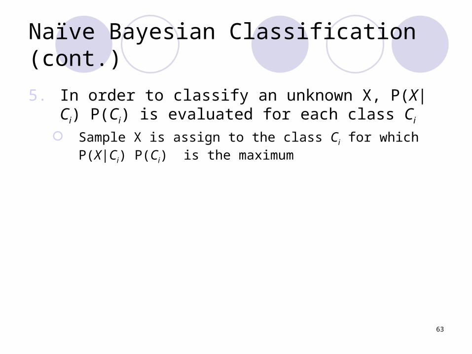
Naïve Bayesian Classification (cont.)
5. In order to classify an unknown X, P(X|Ci) P(Ci) is evaluated for each class Ci
Sample X is assign to the class Ci for which P(X|Ci) P(Ci) is the maximum
64
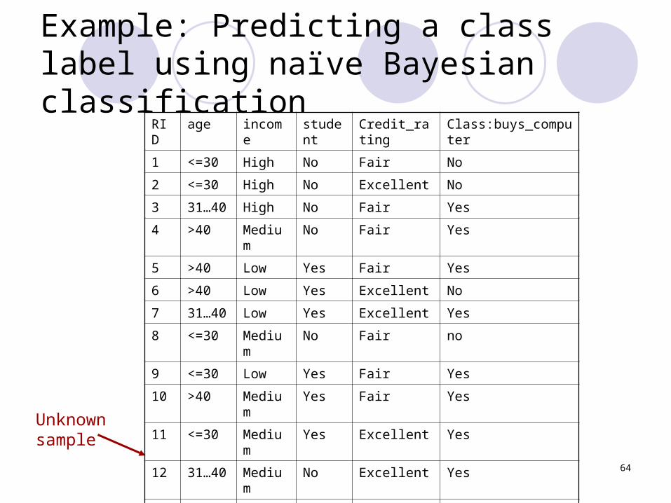
Example: Predicting a class label using naïve Bayesian classification
RID age income student
Credit_rating
Class:buys_computer
1 <=30 High No Fair No
2 <=30 High No Excellent No
3 31…40 High No Fair Yes
4 >40 Medium No Fair Yes
5 >40 Low Yes Fair Yes
6 >40 Low Yes Excellent No
7 31…40 Low Yes Excellent Yes
8 <=30 Medium No Fair no
9 <=30 Low Yes Fair Yes
10 >40 Medium Yes Fair Yes
11 <=30 Medium Yes Excellent Yes
12 31…40 Medium No Excellent Yes
13 31…40 High Yes Fair Yes
14 >40 medium no Excellent No
15 <=30 medium yes fair
Unknown sample
65
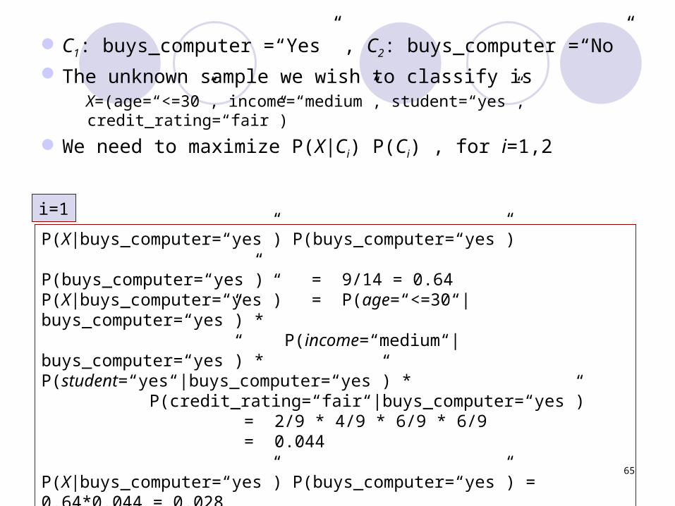
C1: buys_computer =“Yes” , C2: buys_computer =“No”
The unknown sample we wish to classify is X=(age=“<=30”, income=“medium”, student=“yes”,
credit_rating=“fair”)
We need to maximize P(X|Ci) P(Ci) , for i=1,2
P(X|buys_computer=“yes”) P(buys_computer=“yes”)
P(buys_computer=“yes”) = 9/14 = 0.64P(X|buys_computer=“yes”)= P(age=“<=30“|buys_computer=“yes”) *
P(income=“medium“|buys_computer=“yes”) * P(student=“yes“|buys_computer=“yes”) * P(credit_rating=“fair“|buys_computer=“yes”) = 2/9 * 4/9 * 6/9 * 6/9= 0.044
P(X|buys_computer=“yes”) P(buys_computer=“yes”) = 0.64*0.044 = 0.028
i=1

66
P(X|buys_computer=“no”) P(buys_computer=“no”)
P(buys_computer=“no”) = 5/14 = 0.36P(X|buys_computer=“no”) = P(age=“<=30“|buys_computer=“no”) *
P(income=“medium“|buys_computer=“no”) * P(student=“yes“|buys_computer=“no”) * P(credit_rating=“fair“|buys_computer=“no”) = 3/5 * 2/5 * 1/5 * 2/5= 0.019
P(X|buys_computer=“yes”) P(buys_computer=“yes”) = 0.36*0.019= 0.007
i=2
Therefore,
X=(age=“<=30”, income=“medium”, student=“yes”, credit_rating=“fair”) should be in class buys_computer= “yes”
67
Outlook Temperature Humidity Windy Play
Sunny Hot High False N
Sunny Hot High True N
Overcast Hot High False Y
Rainy Mild High False Y
Rainy Cool Normal False Y
Rainy Cool Normal True N
Overcast Cool Normal True Y
Sunny Mild high False N
Sunny Cool Normal False Y
Rainy Mild Normal False Y
Sunny Mild Normal True Y
Overcast Hot Normal False Y
Overcast Mild High True Y
Rainy Mild High True N
Sunny Cool Normal False
Rainy Mild High False
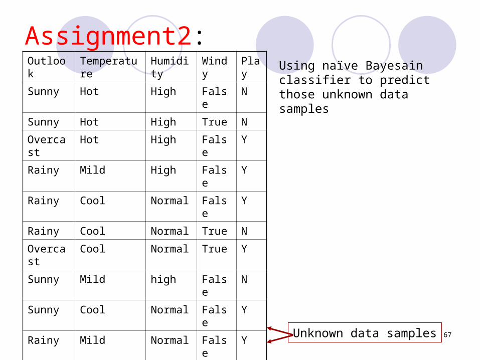
Assignment2:Using naïve Bayesain classifier to predict those unknown data samples
Unknown data samples
68
Prediction: Linear Regression
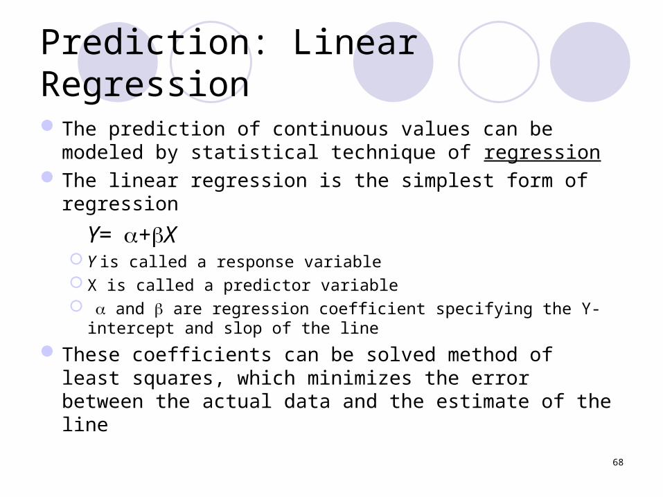
The prediction of continuous values can be modeled by statistical technique of regression
The linear regression is the simplest form of regression
Y=+X Y is called a response variable X is called a predictor variable and are regression coefficient specifying the Y-intercept
and slop of the line
These coefficients can be solved method of least squares, which minimizes the error between the actual data and the estimate of the line

69
Example : Find the linear regression of salary data
Y=+X
= (xi-x)(yi-y) = 3.5
= y - x = 23.6
Predicted line is estimated by
Y = 23.6 + 3.5X
X
Year experience
Y
Salary (in $1000s)
3 30
8 57
9 64
13 72
3 36
6 43
11 59
21 90
1 20
16 83
10 23.6+3.5(10) = 58.6
Salary data
(xi-x)2
s
i=1s
i=1
x = 9.1 and y = 55.4

70
Classifier Accuracy Measures
The accuracy of a classifier on a given test set is the percentage of test set tuples that are correctly classified by the classifier Recognition rate – for pattern recognition literature
The error rate or misclassification rate of the classifier M is simply
1- Acc(M)
where Acc(M) is the accuracy of M If we were to use the training set to estimate the error rate
of the model resubstitution errorConfusion matrix is a useful tool for analyzing how well the
classifier can recognize
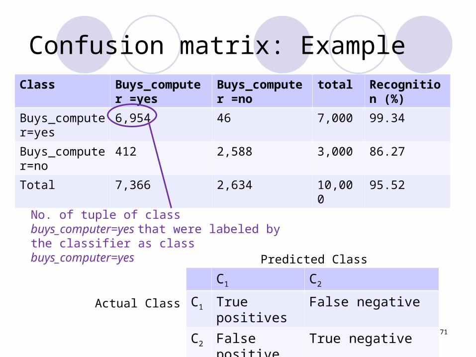
Confusion matrix: ExampleClass Buys_computer
=yesBuys_computer =no
total Recognition (%)
Buys_computer=yes
6,954 46 7,000 99.34
Buys_computer=no
412 2,588 3,000 86.27
Total 7,366 2,634 10,000 95.52
71
No. of tuple of class buys_computer=yes that were labeled by the classifier as class buys_computer=yes
C1 C2
C1 True positives False negative
C2 False positive True negative
Predicted Class
Actual Class

Are there alternatives to the accuracy measure?Are there alternatives to the accuracy measure?Sensitivity refer to true positive (recognition) rate = the
porportion of positive tuples that are correctly idenitfied Specificity is the true negative rate = the proportion of
negative tuples that are correctly identified
72
sensitivity = t_pos / posspecificity = t_neg / negprecision = t_pos / (t_pos+f_pos)Accuracy = sensitivity pos + specificity neg (pos+neg) (pos+neg)
No of positive tuples

Predictor Error Measure
Loss functions measure the error between yi and the predicted value yi’
The most common loss functions are Absolute error: |yi-yi’|
Squared error: (yi-yi’)2
Based on the above, the test error (rate) or generalization error, is the average loss over the test set
Thus, we get the following error rates
Mean absolute error:
Mean squared error: 73
d
yyd
iii
1
d
yyd
iii
1
2
Evaluating the Accuracy of a Classifier or PredictorHow can we use those measures to obtain a reliable
estimate of classifier accuracy (or predictor accuracy)Accuracy estimates can help in comparison of different
classifiersCommon techniques to assessing accuracy based on
randomly sampled partitions of the given data Holdout, random subsamplig, cross-validation, bootstrap
74

75
Evaluating the Accuracy of a Classifier or PredictorHoldout method
The given data are randomly partitioned into 2 independent sets, a training data and a test set
Typically, 2/3 are training set, 1/3 are test set Training set: used to derive the classifier Test set: used to estimate the derived classifier
Data
Training set
Test set
Derived model
Estimate accuracy
Evaluating the Accuracy of a Classifier or PredictorRandom subsampling
The variation of the hold out method Repeat hold out method k times The overall accuracy estimate is the average of the
accuracies obtained from each iteration
76
77
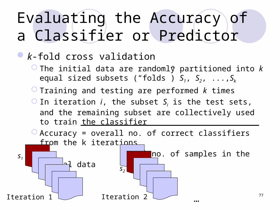
Evaluating the Accuracy of a Classifier or Predictork-fold cross validation
The initial data are randomly partitioned into k equal sized subsets (“folds”) S1, S2, ...,Sk
Training and testing are performed k times In iteration i, the subset Si is the test sets, and the remaining
subset are collectively used to train the classifier Accuracy = overall no. of correct classifiers from the k iterations
total no. of samples in the initial data
Iteration 1
s1
Iteration 2
s2
…
Evaluating the Accuracy of a Classifier or PredictorBootstrap method
The training tuples are sampled uniformly with replacement Each time a tuple is selected, it is equally likely to be selected
again and readded to the training set There are several bootstrap method – the commonly used one
is .632 bootstrap which works as followsGiven a data set of d tuplesThe data set is sampled d times, with replacement, resulting bootstrap sample
of training set of d samples It is very likely that some of the original data tuples will occur more than once in
this sampleThe data tuples that did not make it into the training set end up forming the
test setSuppose we try this out several times – on average 63.2% of original data
tuple will end up in the bootstrap, and the remaining 36.8% will form the test set
78

CLUSTER ANALYSIS
79

80
What is Cluster Analysis
Clustering: the process of grouping the data into classes or clusters which the objects within a cluster have high similarity in comparison to one another, but very dissimilarity to objects in other clusters
What are some typical applications of clustering? In business, discovering distinct groups in their customer bases
and characterize customer groups based on purchasing patterns In biology, derive plant and animal taxonomies, categorize
genes Etc.
Clustering is also call data segmentation in some application because clustering partition large data set into groups according to their similarity
What is Cluster Analysis
Clustering can also be used for outlier detection, where outliers (value that are “far away” from any cluster) may be more interesting than common cases Application- the detection of credit card fraud, monitoring of
criminal activities in electronic commerce
In machine learning, clustering is an example of unsupervised learning (do not rely on predefined classes)
81
82
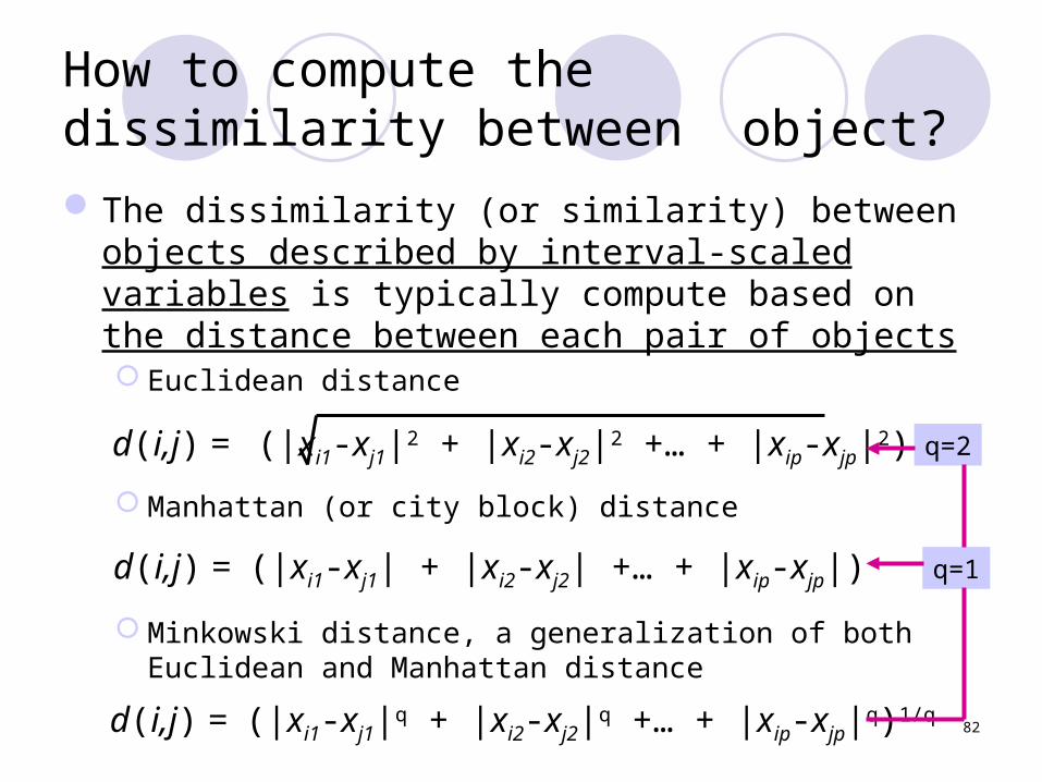
How to compute the dissimilarity between object?
The dissimilarity (or similarity) between objects described by interval-scaled variables is typically compute based on the distance between each pair of objects Euclidean distance
Manhattan (or city block) distance
Minkowski distance, a generalization of both Euclidean and Manhattan distance
d(i,j) = (|xi1-xj1|2 + |xi2-xj2|2 +… + |xip-xjp|2)
d(i,j) = (|xi1-xj1| + |xi2-xj2| +… + |xip-xjp|)
d(i,j) = (|xi1-xj1|q + |xi2-xj2|q +… + |xip-xjp|q)1/q
q=2
q=1

83
Centroid-Based Technique: The K-Means Method
Cluster similarity is measured in regard to the mean value of the objects in a cluster, which can be viewed as the cluster’s centroid or center of gravity
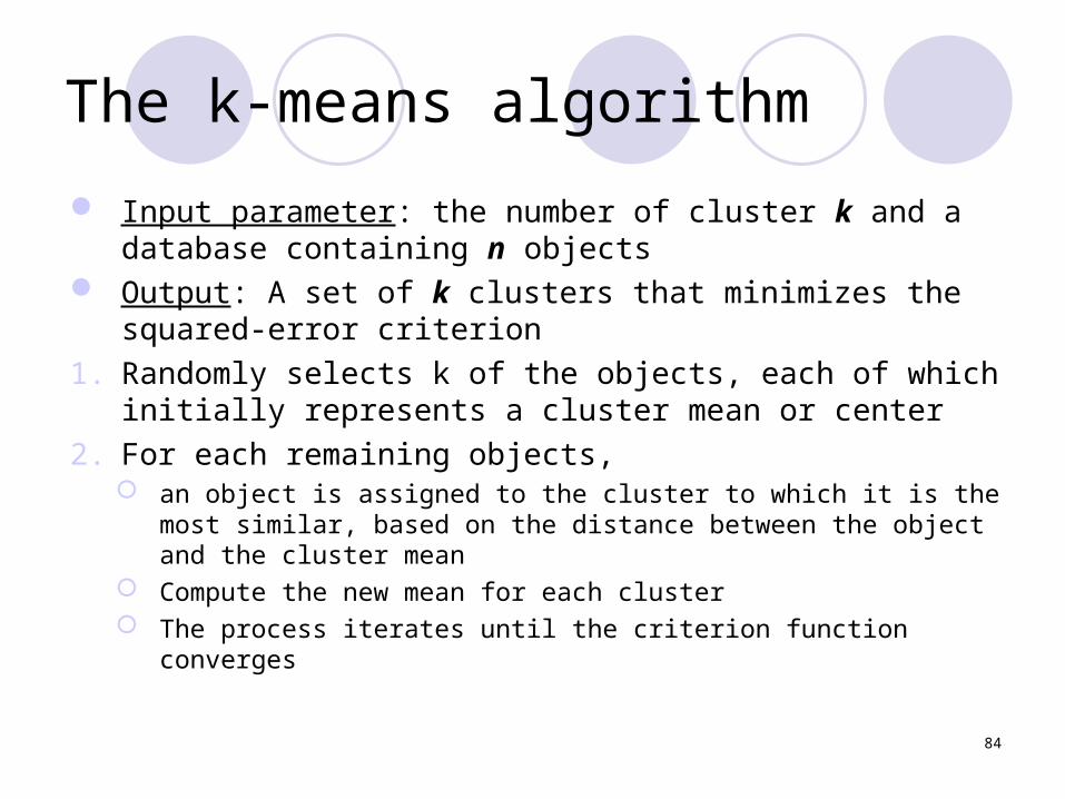
The k-means algorithm
Input parameter: the number of cluster k and a database containing n objects
Output: A set of k clusters that minimizes the squared-error criterion
1. Randomly selects k of the objects, each of which initially represents a cluster mean or center
2. For each remaining objects, an object is assigned to the cluster to which it is the most
similar, based on the distance between the object and the cluster mean
Compute the new mean for each cluster The process iterates until the criterion function converges
84
85
The K-Means Method
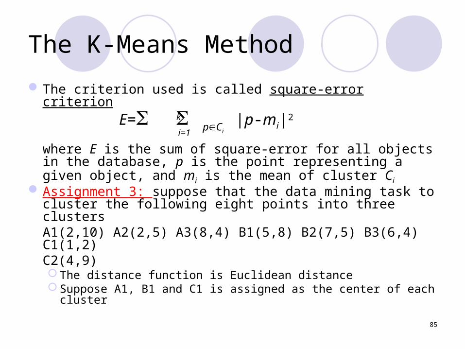
The criterion used is called square-error criterion
where E is the sum of square-error for all objects in the database, p is the point representing a given object, and mi is the mean of cluster Ci
Assignment 3: suppose that the data mining task to cluster the following eight points into three clustersA1(2,10) A2(2,5) A3(8,4) B1(5,8) B2(7,5) B3(6,4) C1(1,2) C2(4,9) The distance function is Euclidean distance Suppose A1, B1 and C1 is assigned as the center of each
cluster
E= |p-mi|2i=1
k pCi