12 – 1 inventory management © 2006 prentice hall, inc

12 – 1

Inventory ManagementInventory Management

© 2006 Prentice Hall, Inc.

12 – 2

InventoryInventory

One of the most expensive assets One of the most expensive assets of many companies representing as of many companies representing as much as 50% of total invested much as 50% of total invested capitalcapital

Operations managers must balance Operations managers must balance inventory investment and customer inventory investment and customer serviceservice

12 – 3

Functions of InventoryFunctions of Inventory

1.1. To decouple or separate various To decouple or separate various parts of the production processparts of the production process

2.2. To decouple the firm from To decouple the firm from fluctuations in demand and fluctuations in demand and provide a stock of goods that will provide a stock of goods that will provide a selection for customersprovide a selection for customers

3.3. To take advantage of quantity To take advantage of quantity discountsdiscounts

4.4. To hedge against inflationTo hedge against inflation

12 – 4

Types of InventoryTypes of Inventory

Raw materialRaw material Purchased but not processedPurchased but not processed

Work-in-processWork-in-process Undergone some change but not completedUndergone some change but not completed A function of cycle time for a productA function of cycle time for a product

Maintenance/repair/operating (MRO)Maintenance/repair/operating (MRO) Necessary to keep machinery and processes Necessary to keep machinery and processes

productiveproductive

Finished goodsFinished goods Completed product awaiting shipmentCompleted product awaiting shipment

12 – 5

The Material Flow CycleThe Material Flow Cycle

InputInput Wait forWait for Wait toWait to MoveMove Wait in queueWait in queue SetupSetup RunRun OutputOutputinspectioninspection be movedbe moved timetime for operatorfor operator timetime timetime

Cycle timeCycle time

95%95% 5%5%

12 – 6

Inventory ManagementInventory Management

How inventory items can be How inventory items can be classifiedclassified

How accurate inventory records How accurate inventory records can be maintainedcan be maintained

12 – 7

ABC AnalysisABC Analysis

Divides inventory into three classes Divides inventory into three classes based on annual dollar volumebased on annual dollar volume Class A - high annual dollar volumeClass A - high annual dollar volume

Class B - medium annual dollar Class B - medium annual dollar volumevolume

Class C - low annual dollar volumeClass C - low annual dollar volume

Used to establish policies that focus Used to establish policies that focus on the few critical parts and not the on the few critical parts and not the many trivial onesmany trivial ones

12 – 8


Item Item Stock Stock

NumberNumber

Percent of Percent of Number of Number of

Items Items StockedStocked

Annual Annual Volume Volume (units)(units) xx

Unit Unit CostCost ==

Annual Annual Dollar Dollar

VolumeVolume

Percent of Percent of Annual Annual Dollar Dollar

VolumeVolume ClassClass

#10286#10286 20%20% 1,0001,000 $ 90.00$ 90.00 $ 90,000$ 90,000 38.8%38.8% 72%72% AA

#11526#11526 500500 154.00154.00 77,00077,000 33.2%33.2% AA

#12760#12760 1,5501,550 17.0017.00 26,35026,350 11.3%11.3% BB

#10867#10867 30%30% 350350 42.8642.86 15,00115,001 6.4%6.4% 23%23% BB

#10500#10500 1,0001,000 12.5012.50 12,50012,500 5.4%5.4% BB

12 – 9


Item Item Stock Stock

NumberNumber

Percent of Percent of Number of Number of

Items Items StockedStocked

Annual Annual Volume Volume (units)(units) xx

Unit Unit CostCost ==

Annual Annual Dollar Dollar

VolumeVolume

Percent of Percent of Annual Annual Dollar Dollar

VolumeVolume ClassClass

#12572#12572 600600 $ 14.17$ 14.17 $ 8,502$ 8,502 3.7%3.7% CC

#14075#14075 2,0002,000 .60.60 1,2001,200 .5%.5% CC

#01036#01036 50%50% 100100 8.508.50 850850 .4%.4% CC

#01307#01307 1,2001,200 .42.42 504504 .2%.2% CC

#10572#10572 250250 .60.60 150150 .1%.1% CC

12 – 10


A ItemsA Items

B ItemsB ItemsC ItemsC Items

Pe

rce

nt

of

an

nu

al d

olla

r u

sa

ge

Pe

rce

nt

of

an

nu

al d

olla

r u

sa

ge

80 80 –

70 70 –

60 60 –

50 50 –

40 40 –

30 30 –

20 20 –

10 10 –

0 0 – | | | | | | | | | |

1010 2020 3030 4040 5050 6060 7070 8080 9090 100100

Percent of inventory itemsPercent of inventory items

12 – 11


Other criteria than annual dollar Other criteria than annual dollar volume may be usedvolume may be used Anticipated engineering changesAnticipated engineering changes

Delivery problemsDelivery problems

Quality problemsQuality problems

High unit costHigh unit cost

12 – 12


Policies employed may includePolicies employed may include More emphasis on supplier More emphasis on supplier

development for A itemsdevelopment for A items

Tighter physical inventory control for Tighter physical inventory control for A itemsA items

More care in forecasting A itemsMore care in forecasting A items

12 – 13

Record AccuracyRecord Accuracy Accurate records are a critical Accurate records are a critical

ingredient in production and inventory ingredient in production and inventory systemssystems

Allows organization to focus on what Allows organization to focus on what is neededis needed

Necessary to make precise decisions Necessary to make precise decisions about ordering, scheduling, and about ordering, scheduling, and shippingshipping

Incoming and outgoing record Incoming and outgoing record keeping must be accuratekeeping must be accurate

Stockrooms should be secureStockrooms should be secure

12 – 14

Cycle CountingCycle Counting Items are counted and records updated Items are counted and records updated

on a periodic basison a periodic basis

Often used with ABC analysis to Often used with ABC analysis to determine cycledetermine cycle

Has several advantagesHas several advantages Eliminates shutdowns and interruptionsEliminates shutdowns and interruptions

Eliminates annual inventory adjustmentEliminates annual inventory adjustment

Trained personnel audit inventory accuracyTrained personnel audit inventory accuracy

Allows causes of errors to be identified and Allows causes of errors to be identified and correctedcorrected

Maintains accurate inventory recordsMaintains accurate inventory records

12 – 15

Cycle Counting ExampleCycle Counting Example

5,000 items in inventory, 500 A items, 1,750 B items, 2,750 C 5,000 items in inventory, 500 A items, 1,750 B items, 2,750 C itemsitems

Policy is to count A items every month (20 working days), B Policy is to count A items every month (20 working days), B items every quarter (60 days), and C items every six months items every quarter (60 days), and C items every six months (120 days)(120 days)

Item Item ClassClass QuantityQuantity Cycle Counting PolicyCycle Counting Policy

Number of Items Number of Items Counted per DayCounted per Day

AA 500500 Each monthEach month 500/20 = 25/500/20 = 25/dayday

BB 1,7501,750 Each quarterEach quarter 1,750/60 = 29/1,750/60 = 29/dayday

CC 2,7502,750 Every 6 monthsEvery 6 months 2,750/120 = 23/2,750/120 = 23/dayday

77/77/dayday

12 – 16

Independent Versus Independent Versus Dependent DemandDependent Demand

Independent demand - the Independent demand - the demand for item is independent demand for item is independent of the demand for any other of the demand for any other item in inventoryitem in inventory

Dependent demand - the Dependent demand - the demand for item is dependent demand for item is dependent upon the demand for some upon the demand for some other item in the inventoryother item in the inventory

12 – 17

Holding, Ordering, and Holding, Ordering, and Setup CostsSetup Costs

Holding costs - the costs of holding Holding costs - the costs of holding or “carrying” inventory over timeor “carrying” inventory over time

Ordering costs - the costs of Ordering costs - the costs of placing an order and receiving placing an order and receiving goodsgoods

Setup costs - cost to prepare a Setup costs - cost to prepare a machine or process for machine or process for manufacturing an ordermanufacturing an order

12 – 18

Holding CostsHolding Costs

CategoryCategory

Cost (and Range) Cost (and Range) as a Percent of as a Percent of Inventory ValuInventory Valuee

Housing costs (including rent or Housing costs (including rent or depreciation, operating costs, taxes, depreciation, operating costs, taxes, insurance)insurance)

6%6% (3 - 10%) (3 - 10%)

Material handling costs (equipment lease or Material handling costs (equipment lease or depreciation, power, operating cost)depreciation, power, operating cost)

3%3% (1 - 3.5%) (1 - 3.5%)

Labor costLabor cost 3%3% (3 - 5%) (3 - 5%)

Investment costs (borrowing costs, taxes, Investment costs (borrowing costs, taxes, and insurance on inventory)and insurance on inventory)

11%11% (6 - 24%) (6 - 24%)

Pilferage, space, and obsolescencePilferage, space, and obsolescence 3%3% (2 - 5%) (2 - 5%)

Overall carrying costOverall carrying cost 26%26%

12 – 19

Inventory Models for Inventory Models for Independent DemandIndependent Demand

Basic economic order quantityBasic economic order quantity

Production order quantityProduction order quantity

Quantity discount modelQuantity discount model

Need to determine when and how Need to determine when and how much to ordermuch to order

12 – 20

Basic EOQ ModelBasic EOQ Model

1.1. Demand is known, constant, and Demand is known, constant, and independentindependent

2.2. Lead time is known and constantLead time is known and constant

3.3. Receipt of inventory is instantaneous and Receipt of inventory is instantaneous and completecomplete

4.4. Quantity discounts are not possibleQuantity discounts are not possible

5.5. Only variable costs are setup and holdingOnly variable costs are setup and holding

6.6. Stockouts can be completely avoidedStockouts can be completely avoided

Important assumptionsImportant assumptions

12 – 21

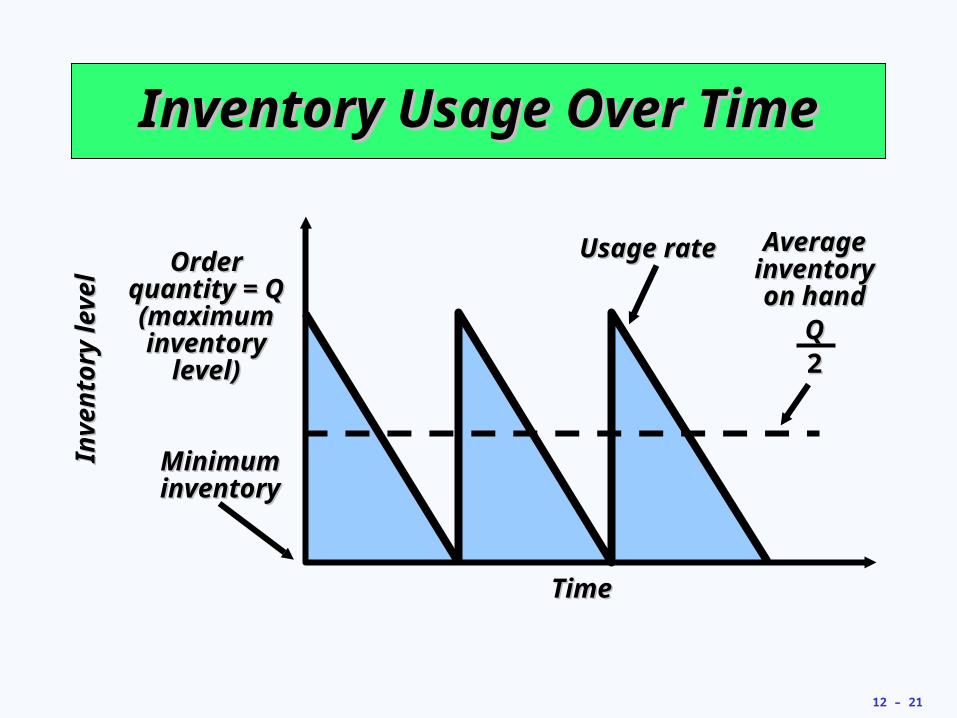
Inventory Usage Over TimeInventory Usage Over Time

Order Order quantity = Q quantity = Q (maximum (maximum inventory inventory

level)level)

Inve

nto

ry le

vel

Inve

nto

ry le

vel

TimeTime

Usage rateUsage rate Average Average inventory inventory on handon hand

QQ22

Minimum Minimum inventoryinventory

12 – 22

Minimizing CostsMinimizing Costs

Objective is to minimize total costsObjective is to minimize total costs

An

nu

al c

ost

An

nu

al c

ost

Order quantityOrder quantity

Curve for total Curve for total cost of holding cost of holding

and setupand setup

Holding cost Holding cost curvecurve

Setup (or order) Setup (or order) cost curvecost curve

Minimum Minimum total costtotal cost

Optimal Optimal order order

quantityquantity

12 – 23

The EOQ ModelThe EOQ Model

QQ = Number of pieces per order= Number of pieces per orderQ*Q* = Optimal number of pieces per order (EOQ)= Optimal number of pieces per order (EOQ)DD = Annual demand in units for the Inventory item= Annual demand in units for the Inventory itemSS = Setup or ordering cost for each order= Setup or ordering cost for each orderHH = Holding or carrying cost per unit per year= Holding or carrying cost per unit per year

Annual setup cost Annual setup cost == ((Number of orders placed per yearNumber of orders placed per year) ) x (x (Setup or order cost per orderSetup or order cost per order))

Annual demandAnnual demand

Number of units in each orderNumber of units in each orderSetup or order Setup or order cost per ordercost per order

==

= (= (SS))DDQQ

Annual setup cost = SDQ

12 – 24



Annual holding cost Annual holding cost == ((Average inventory levelAverage inventory level) ) x (x (Holding cost per unit per yearHolding cost per unit per year))

Order quantityOrder quantity

22= (= (Holding cost per unit per yearHolding cost per unit per year))

= (= (HH))QQ22


Annual holding cost = HQ2

12 – 25



Optimal order quantity is found when annual setup cost Optimal order quantity is found when annual setup cost equals annual holding costequals annual holding cost


Annual holding cost = HQ2

DDQQ

SS = = HHQQ22

Solving for Q*Solving for Q*22DS = QDS = Q22HHQQ22 = = 22DS/HDS/H

Q* = Q* = 22DS/HDS/H

12 – 26

An EOQ ExampleAn EOQ Example

Determine optimal number of needles to orderDetermine optimal number of needles to orderD D = 1,000= 1,000 units unitsS S = $10= $10 per order per orderH H = $.50= $.50 per unit per year per unit per year

Q* =Q* =22DSDS

HH

Q* =Q* =2(1,000)(10)2(1,000)(10)

0.500.50= 40,000 = 200= 40,000 = 200 units units

12 – 27


Determine optimal number of needles to orderDetermine optimal number of needles to orderD D = 1,000= 1,000 units units Q* Q* = 200= 200 units unitsS S = $10= $10 per order per orderH H = $.50= $.50 per unit per year per unit per year

= N = == N = =Expected Expected number of number of

ordersorders

DemandDemandOrder quantityOrder quantity

DDQ*Q*

N N = = 5= = 5 orders per year orders per year 1,0001,000200200

12 – 28


Determine optimal number of needles to orderDetermine optimal number of needles to orderD D = 1,000= 1,000 units units Q*Q* = 200= 200 units unitsS S = $10= $10 per order per order NN = 5= 5 orders per year orders per yearH H = $.50= $.50 per unit per year per unit per year

= T == T =Expected Expected

time between time between ordersorders

Number of working Number of working days per yeardays per year

NN

T T = = 50 = = 50 days between ordersdays between orders250250

55

12 – 29


Determine optimal number of needles to orderDetermine optimal number of needles to orderD D = 1,000= 1,000 units units Q*Q* = 200= 200 units unitsS S = $10= $10 per order per order NN = 5= 5 orders per year orders per yearH H = $.50= $.50 per unit per year per unit per year TT = 50= 50 days days

Total annual cost = Setup cost + Holding costTotal annual cost = Setup cost + Holding cost

TC = S + HTC = S + HDDQQ

QQ22

TC TC = ($10) + ($.50)= ($10) + ($.50)1,0001,000200200

20020022

TC TC = (5)($10) + (100)($.50) = $50 + $50 = $100= (5)($10) + (100)($.50) = $50 + $50 = $100

12 – 30

Robust ModelRobust Model

The EOQ model is robustThe EOQ model is robust

It works even if all parameters It works even if all parameters and assumptions are not metand assumptions are not met

The total cost curve is relatively The total cost curve is relatively flat in the area of the EOQflat in the area of the EOQ

12 – 31


Management underestimated demand by 50%Management underestimated demand by 50%D D = 1,000= 1,000 units units Q*Q* = 200= 200 units unitsS S = $10= $10 per order per order NN = 5= 5 orders per year orders per yearH H = $.50= $.50 per unit per year per unit per year TT = 50= 50 days days


QQ22

TC TC = ($10) + ($.50) = $75 + $50 = $125= ($10) + ($.50) = $75 + $50 = $1251,5001,500200200

20020022

1,500 1,500 unitsunits

Total annual cost increases by only 25%Total annual cost increases by only 25%

12 – 32


Actual EOQ for new demand is Actual EOQ for new demand is 244.9244.9 units unitsD D = 1,000= 1,000 units units Q*Q* = 244.9= 244.9 units unitsS S = $10= $10 per order per order NN = 5= 5 orders per year orders per yearH H = $.50= $.50 per unit per year per unit per year TT = 50= 50 days days


QQ22

TC TC = ($10) + ($.50)= ($10) + ($.50)1,5001,500244.9244.9

244.9244.922

1,500 1,500 unitsunits

TC TC = $61.24 + $61.24 = $122.48= $61.24 + $61.24 = $122.48

Only 2% less than the total cost of $125

when the order quantity

was 200

12 – 33

Reorder PointsReorder Points

EOQ answers the “how much” questionEOQ answers the “how much” question

The reorder point (ROP) tells when to The reorder point (ROP) tells when to orderorder

ROP ROP ==Lead time for a Lead time for a

new order in daysnew order in daysDemand Demand per dayper day

== d x L d x L

d = d = DDNumber of working days in a yearNumber of working days in a year

12 – 34

Reorder Point CurveReorder Point Curve

Q*Q*

ROP ROP (units)(units)In

ven

tory

lev

el (

un

its)

Inve

nto

ry l

evel

(u

nit

s)

Time (days)Time (days)Lead time = LLead time = L

Slope = units/day = dSlope = units/day = d

12 – 35

Reorder Point ExampleReorder Point Example

Demand Demand = 8,000= 8,000 DVDs per year DVDs per year250250 working day year working day yearLead time for orders is Lead time for orders is 33 working days working days

ROP =ROP = d x L d x L

d =d = DD

Number of working days in a yearNumber of working days in a year

= 8,000/250 = 32= 8,000/250 = 32 units units

= 32= 32 units per day x units per day x 33 days days = 96= 96 units units

12 – 36

Production Order Quantity Production Order Quantity ModelModel

Used when inventory builds up over Used when inventory builds up over a period of time after an order is a period of time after an order is placedplaced

Used when units are produced and Used when units are produced and sold simultaneouslysold simultaneously

12 – 37


Inve

nto

ry l

evel

Inve

nto

ry l

evel

TimeTime

Demand part of cycle Demand part of cycle with no productionwith no production

Part of inventory cycle during Part of inventory cycle during which production (and usage) which production (and usage) is taking placeis taking place

tt

Maximum Maximum inventoryinventory

12 – 38


Q =Q = Number of pieces per orderNumber of pieces per order p = p = Daily production rateDaily production rateH =H = Holding cost per unit per yearHolding cost per unit per year d = d = Daily demand/usage rateDaily demand/usage ratet =t = Length of the production run in daysLength of the production run in days

= (= (Average inventory levelAverage inventory level)) x xAnnual inventory Annual inventory holding costholding cost

Holding cost Holding cost per unit per yearper unit per year

= (= (Maximum inventory levelMaximum inventory level)/2)/2Annual inventory Annual inventory levellevel

= –= –Maximum Maximum inventory levelinventory level

Total produced during Total produced during the production runthe production run

Total used during Total used during the production runthe production run

== pt – dt pt – dt

12 – 39


Q =Q = Number of pieces per orderNumber of pieces per order p = p = Daily production rateDaily production rateH =H = Holding cost per unit per yearHolding cost per unit per year d = d = Daily demand/usage rateDaily demand/usage ratet =t = Length of the production run in daysLength of the production run in days

= –= –Maximum Maximum inventory levelinventory level

Total produced during Total produced during the production runthe production run

Total used during Total used during the production runthe production run

== pt – dt pt – dt

However, Q = total produced = pt ; thus t = Q/pHowever, Q = total produced = pt ; thus t = Q/p

Maximum Maximum inventory levelinventory level = p – d = Q = p – d = Q 1 –1 –QQ

ppQQpp

ddpp

Holding cost = Holding cost = ((HH)) = = 1 –1 – H H ddpp

QQ22

Maximum inventory levelMaximum inventory level

22

12 – 40


Q =Q = Number of pieces per orderNumber of pieces per order p = p = Daily production rateDaily production rateH =H = Holding cost per unit per yearHolding cost per unit per year d = d = Daily demand/usage rateDaily demand/usage rateD =D = Annual demandAnnual demand

Setup cost Setup cost == ((DD//QQ))SS

Holding cost Holding cost == 1/21/2 HQ HQ[1 - ([1 - (dd//pp)])]

((DD//QQ))S = S = 1/21/2 HQ HQ[1 - ([1 - (dd//pp)])]

QQ22 = =22DSDS

HH[1 - ([1 - (dd//pp)])]

QQ* =* =22DSDS

HH[1 - ([1 - (dd//pp)])]

12 – 41

Production Order Quantity Production Order Quantity ExampleExample

D D == 1,0001,000 units units p p == 88 units per day units per dayS S == $10$10 d d == 44 units per day units per dayH H == $0.50$0.50 per unit per year per unit per year

QQ* =* =22DSDS

HH[1 - ([1 - (dd//pp)])]

= 282.8 = 282.8 oror 283 283 hubcapshubcaps

QQ* = = 80,000* = = 80,0002(1,000)(10)2(1,000)(10)

0.50[1 - (4/8)]0.50[1 - (4/8)]

12 – 42


When annual data are used the equation becomesWhen annual data are used the equation becomes

QQ* =* =22DSDS

annual demand rateannual demand rateannual production rateannual production rateH H 1 –1 –

12 – 43

Probabilistic Models and Probabilistic Models and Safety StockSafety Stock

Used when demand is not constant or Used when demand is not constant or certaincertain

Use safety stock to achieve a desired Use safety stock to achieve a desired service level and avoid stockoutsservice level and avoid stockouts

ROP ROP == d x L d x L + + ssss

Annual stockout costs = the sum of the units short Annual stockout costs = the sum of the units short x the probability x the stockout cost/unit x the probability x the stockout cost/unit

x the number of orders per yearx the number of orders per year

12 – 44

Safety stock 16.5 units

ROP ROP

Place Place orderorder

Probabilistic DemandProbabilistic DemandIn

ven

tory

lev

elIn

ven

tory

lev

el

TimeTime00

Minimum demand during lead timeMinimum demand during lead time

Maximum demand during lead timeMaximum demand during lead time

Mean demand during lead timeMean demand during lead time

Normal distribution probability of Normal distribution probability of demand during lead timedemand during lead time

Expected demand during lead time Expected demand during lead time (350(350 kits kits))

ROP ROP = 350 += 350 + safety stock of safety stock of 16.5 = 366.516.5 = 366.5

Receive Receive orderorder

Lead Lead timetime

12 – 45

Probabilistic DemandProbabilistic Demand

Safety Safety stockstock

Probability ofProbability ofno stockoutno stockout

95% of the time95% of the time

Mean Mean demand demand

350350

ROP = ? kitsROP = ? kits QuantityQuantity

Number of Number of standard deviationsstandard deviations

00 zz

Risk of a stockout Risk of a stockout (5% of area of (5% of area of normal curve)normal curve)

12 – 46

Probabilistic DemandProbabilistic Demand

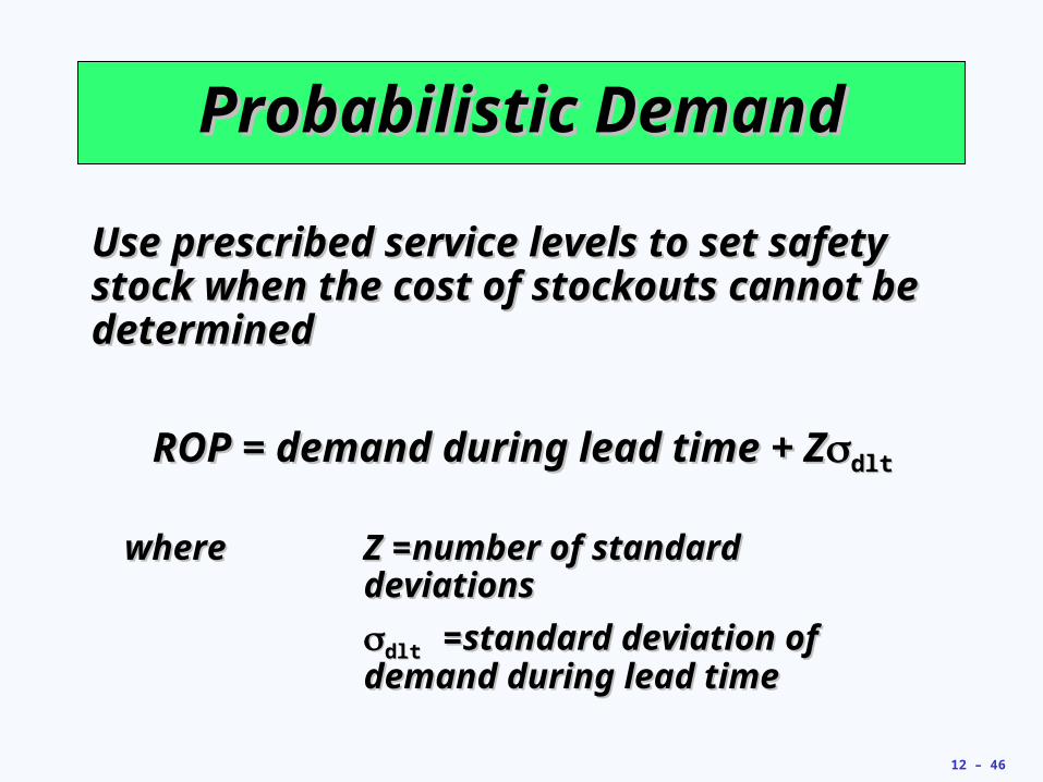
Use prescribed service levels to set safety Use prescribed service levels to set safety stock when the cost of stockouts cannot be stock when the cost of stockouts cannot be determineddetermined

ROP = demand during lead time + ZROP = demand during lead time + Zdltdlt

wherewhere Z Z ==number of standard number of standard deviationsdeviations

dltdlt = =standard deviation of standard deviation of demand during lead timedemand during lead time

12 – 47

EOQ FallaciesEOQ Fallacies

• Unit Price always fixedUnit Price always fixed

• All resAll resources related to inventory are ources related to inventory are sufficientsufficient

• Order can be fractionalizedOrder can be fractionalized

• Unrealistic assumptionsUnrealistic assumptions

• Items are IndependentItems are Independent

• Storage Policy is assumed to be Storage Policy is assumed to be randomizedrandomized

12 – 48

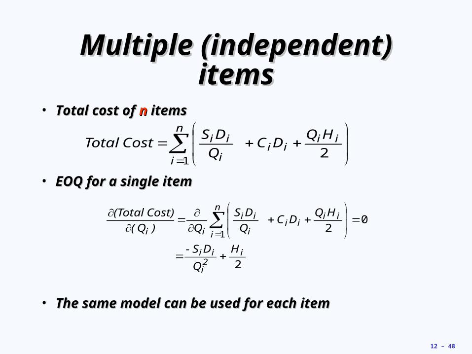
Multiple (independent) itemsMultiple (independent) items

• Total cost of Total cost of nn items items

• EOQ for a single itemEOQ for a single item

• The same model can be used for each itemThe same model can be used for each item

n

i

iiii

i

ii HQDC

Q

DS Cost Total

12

2

02

1

i2i

ii

n

i

iiii

i

ii

ii

H

Q

DS-

HQDC

Q

DS

Q

)Q(

Cost) (Total

12 – 49

Multiple (dependent) itemsMultiple (dependent) items

• Assume that each unit of item i Assume that each unit of item i requiresrequires ffii square feetsquare feet of storage of storage space and the total of space and the total of FF square feet square feet is availableis available

• The EOQ Model is then subjected toThe EOQ Model is then subjected to

FQfn

iii

1

12 – 50


• The Order quantity for each item i The Order quantity for each item i can be found by applying the can be found by applying the Lagrangian Relaxation :Lagrangian Relaxation : L functionL function

n

iii

n

i

iiii

i

ii

n

FQfHQ

DCQ

DS

)Q,...,Q,(L Cost Total Minimize

11

1

2

12 – 51


• EOQ for each single item can be EOQ for each single item can be found fromfound from

• Then,Then,

02

0

ii

2i

ii

ii

fH

Q

DS-

Q

L

)Q(

Cost) (Total

ii

iii fH

DSQ

22

12 – 52


• To find all QTo find all Qii’s’s thatthat satisfy the satisfy the constraint of storage space F, the constraint of storage space F, the search for appropriate value of search for appropriate value of is is requiredrequired

12 – 1 inventory management © 2006 prentice hall, inc

Documents