Income Convergence in South Africa:

Fact or Measurement Error?1

Tobias Lechtenfeld Asmus Zoch2 World Bank Stellenbosch University

Washington, D.C. South Africa

ABCA Conference Paper, PARIS

June 2014

Abstract

This paper asks whether income mobility in South Africa over the last decade has indeed

been as impressive as currently thought. Using new national panel data (NIDS),

substantial measurement error in reported income data is found, which is further

corroborated by a provincial income data panel (KIDS). By employing an instrumental

variables approach using two different instruments, measurement error can be quantified.

Specifically, self-reported income in the survey data is shown to suffer from mean-

reverting measurement bias, leading to sizable overestimations of income convergence in

both panel data sets. The preferred estimates indicate that previously published income

dynamics may have been largely overestimated by as much as 77% for the national NIDS

panel and 39% for the provincial KIDS panel. Overall, income mobility appears much

smaller than previously thought, while chronic poverty remains substantial and transitory

poverty is still very limited in South Africa.

JEL Classifications: C81, I32, O15

Keywords: Measurement Error, Income Dynamics, Consumption Dynamics, South Africa

1 Acknowledgements: We thank Stephan Klasen and Servaas van der Berg for their support

throughout this project. The research for this project was partly conducted while both authors

where with the University of Göttingen, Germany. 2 Correspondence: Asmus Zoch, Stellenbosch University, South Africa. Email:

asmuszoch@gmail.com

1

1. Introduction

The measurement of income dynamics lies at the heart of development economics and is

of great concern to researches and policy makers alike. The collection of panel data in

many developing countries has allowed tremendous progress in this regard. While

progress in poverty alleviation and income mobility is important, it remains unclear just

how much these dynamics are affected by measurement error. The standard measure of

income mobility is the slope coefficient from a regression of current period earnings on

lagged earnings. It is well known that the collection of income and consumption data in

household surveys is often very imprecise. In the presence of classical measurement error

this will cause an attenuation bias towards zero in the estimated slope coefficient,

overstating the degree of mobility. The results are what is being referred to as convergence

towards the mean (Fields et al. 2003, Antman and Mckenzie, 2005). This paper aims to

identify the effect of measurement error when estimating income dynamics.

Twenty years after the end of the apartheid era, South Africa is still characterized by

extremely high inequality. Even more, the overall Gini coefficient for South Africa

increased from 0.67 in 1993 to 0.70 in 2008. During apartheid the high overall level of

inequality was driven by inequality between races. Today there is rising inequality within

the racial groups (e.g. the Gini coefficient for the black population increased from 0.55 in

1993 to 0.62 in 2008) (Leibbrandt et al. 2011). Despite the positive indication that wealth

and poverty are being distributed less along racial lines today and that a new affluent

black elite and middle class have come into being, there seems to be another part of the

black population that is falling behind in relative terms, e.g. Adato et al. (2006) show that

there is an asset level below which households are trapped in poverty. These findings are

in sharp contrast to other literature on South Africa that has found high mobility and

convergence to the mean (Fields et al. 2003a and 2003b, Finn and Leibbrandt 2013).

This paper aims to address this apparent contradiction by estimating the effect of

measurement error in two prominent datasets from South Africa. The two panels are the

National Income Dynamics Survey (NIDS) covering the period 2008-2012, and the smaller

KwaZulu-Natal Income Dynamics Study (KIDS) covering the period of 1993-2004 for only

one province. Using the KIDS data, Fields et al. (2003a and 2003b) and Woolard and

Klasen (2005) previously found strong signs of income convergence. However, the authors

also highlighted the problem of measurement error that could bias their results.

2

This paper is adding to a growing body of literature on income measurement by enhancing

the linear dynamic panel model by allowing for the potential existence of measurement

error. Specifically, an instrumental variable approach is used which controls for

measurement error by instrumenting the initial income variable. The present paper tests

two different instruments, lagged income and household wealth. The use of instruments

is particularly valuable to the analysis of income convergence because it allows an

estimation of both (i) the direction and (ii) the size of the measurement error.

The initial income variable is shown to be endogenous, which implies that measurement

error is indeed a problem in the data and that standard linear panel models do not provide

consistent estimates. The results suggest that estimates that do not control for

measurement error may suffer from substantial bias. Between a third and half of the naïve

estimates of income convergence is found to be a result of measurement error. The

magnitude of these findings suggests that the degree of income mobility is overestimated

in South Africa. The results are robust to different choices of instrumental variables and

holds for both the provincial and national South African panel surveys.

The remainder of this paper is structured as follows: Section 2 provides an overview of the

literature. Section 3 briefly discusses the data followed by an outline of the empirical

strategy, including a discussion of possible robustness checks. Section 4 presents the

results. Section 5 offers some concluding remarks.

2. Theory and Literature Review

This section provides a review of the empirical literature on the effect of measurement

error and poverty dynamics with a focus on South Africa. The problem of potential

measurement error in the existing income panel data has been well recognized in the

literature concerned with poverty dynamics in South Africa (see Agüero et al. 2007, Fields

et al. 2003a and 2003b, and Woolard and Klasen 2005). However, an absence of adequate

remedies in these datasets did not allow a detailed analysis of or avoidance of any bias

stemming from these.

2.1 Income Measurement in South Africa

Woolard and Klasen (2005) in particular emphasized the risk of obtaining biased estimates

of income dynamics when the data erroneously cause income regressions to convert

3

towards the mean. The bias makes results appear as if large numbers of poor households

benefited from income mobility. This is in fact a result found by much of the existing

literature, which suggests that income mobility in developing countries is higher than in

industrialized countries, especially at the poor end of the income distribution (Woolard

and Klasen 2005, p.869). Thus, to obtain a valid picture of income mobility, potential

measurement error needs to be taken into account, a challenge which most of the existing

literature has highlighted. Fields et al. (2003a) stress that income measurement errors

can be of serious concern in developing countries. As Agüero et al. (2007) point out, the

problem occurs when income or expenditure are measured with errors, i.e. the observed

data are “noisy”. This means that panel data will incorrectly show households with stable

incomes changing their position along the income distribution. While the effect on incomes

in the middle of the distribution will be somewhat random, incomes at the tails of the

distribution will be predominantly biased towards the mean. In other words, income

measurement errors in panel data tend to make poor households look better off, and rich

households worse off. In other words “[…] measurement error in initial income contributes

to an apparent negative correlation between base-year income and subsequent income

change” (Fields et al., 2003a, 87).

Following a methodology introduced by Glewwe (2005) to expose measurement errors,

Agüero et al. (2007) note that measurement error could account for up to 60% of previously

found income mobility between 1993 and 1998, using KIDS data. Similarly, Woolard and

Klasen (2005) observe large differences in welfare trends when comparing income and

expenditure measures. These discrepancies indicate that measurement error may indeed

play an important role when analysing income dynamics in South Africa. Despite these

indications, Fields et al. (2003a and 2003b) conclude that even though measurement error

may bias income predictions, true income has likely converged in South Africa and that

their main findings are robust to measurement error.

This paper contributes to the existing literature by using the recently expanded national

NIDS panel dataset for South Africa to re-assess income dynamics and to quantify the

likely bias caused by measurement error. While some of the existing literature has

analysed South African income mobility using NIDS data3, this paper is the first to explore

the possible impact of measurement error on existing results.

3 See for example Finn et al., 2013 or Finn and Leibbrandt, 2013.

4

2.2 Problems in measuring income mobility

In most of the literature from industrialized countries, income mobility of individuals

rather than households is analyzed. Most commonly, income dynamics are estimated

using the variance component model proposed by Lillard and Willis (1978).4 The model

includes a standard income function and an error structure allowing for individual random

effect and first order autocorrelation of a transitory component. It does not include any

lagged dependent variable. Other models assume unobserved heterogeneity to be time-

invariant and include first differences. Under such setting the permanent component of

income inequality cannot be identified.5 Very few existing articles address the

measurement error issue (Baulch and Hoddinott 2000). An exception is the work by

Pischke (1995), who uses administrative data to quantify the effect of measurement error

in self-reported income data.6

In contrast, literature from developing countries tend to estimate income mobility using

measures derived from household income, such as per capita household income.7 When

defining income mobility as ∆Yi,t ≡ Y2 – Y1 to determine how initial income influences

income change, most researchers use income models of the following form:

∆Yi,t ≡ Y2 – Y1=α + β1Yi,t-1 + β2Zi, + β3Xi,t-1 + β4Xi,t + εi,t (1)

These models are straightforward to interpret and provide a measure of convergence.

When β1<0, incomes are exhibiting conditional convergence, while when β1>0, conditional

divergence takes place. Empirically, the existing literature from developing countries has

mostly found that β1<0, which implies that incomes converge to the conditional mean (e.g.

Fields et al., 2003a, Woolard and Klasen 2005, Fields and Puerta, 2010). However, when

incomeY1of the base year is measured with error, such error is present on both sides of the

regression equation (1), which will produce a downward-bias (attenuation) and

inconsistent parameter estimates of the true effect. As previous research has pointed out,

the convergence found in existing studies could be the result of measurement error rather

than a closing of the income gap (Fields, 2008). To address measurement error in the

absence of administrative data, several studies use predicted income to replace Y1on the

4 The model is also referred to as autocorrelated individual component model. 5 McCurdy (1982) uses this approach and tries to improve the model using time series processes

and taking first differences. 6 Pischke (1995) analyses the Panel Study of Income Dynamics Validation Study (PSIDVS).

Similarly, Gottschalk and Huynh (2006) and Dragoset and Fields (2006) use tax records from the

Detailed Earnings Record (DER). 7 See Baulch and Hoddinott (2000) for a literature review on economic mobility and poverty

dynamics.

5

right hand side of the equation (1), where the prediction is based on household or

individual characteristics such as age, education, sector of occupation and dwelling

characteristics (e.g. Fields et al., 2003a, Fields et al., 2010).

A very nascent literature has also shown the existence of nonlinear relationships between

current and lagged income. Lokshin and Ravallion (2004) study poverty traps and report

nonlinear income dynamics for Hungary and Russia. However, their analysis does not

control for potential measurement error. Antman and McKenzie (2007a&2007b)

investigate the nonlinear relationship between current and lagged income and allow for

unobserved heterogeneity and measurement error by using a pseudo-panel approach. This

method assumes that the mean of measurement error across cohorts converges to zero as

the number of individuals within a cohort increases. The authors show that with larger

sample size this approach yields consistent estimates, although the magnitude of existing

measurement errors cannot be quantified.8

Most similar to this paper is the work by Newhouse (2005), who estimates income

dynamics in Indonesia and addresses non-random income measurement error and

unobserved household heterogeneity by using several instruments, including rainfall,

assets and consumption.

In conclusion, very few studies explicitly control for measurement error and estimate the

size and direction of the effect. The analysis below aims to shed additional light on this.

Lastly, for most developing countries administrative income data, such as tax records or

other official income statements, remain largely unavailable or incomplete. Such data

would provide an alternative to self-reported survey data for estimating income

convergence, even though such data would come with its own caveats.

3. Data and Analysis

3.1 South African Panel Data

8 Their studies correct for bias even from non-classical measurement error but, like Lokshin and

Ravallion (2004)’s study, find no evidence for the existence of a poverty trap.

6

To measure poverty dynamics while controlling for unobservable heterogeneity, household

panel data is needed. The two panel studies used in this paper are the National Income

Dynamics Survey (NIDS) and the KwaZulu-Natal Income Dynamics Study (KIDS).

The main rationale for using NIDS is its coverage of the entire country. After the release

of the new 2012 data set, NIDS now contains a three wave panel spanning a time period

of four years. NIDS is quite large, including 26,776 completed individual interviews in

2008 (wave 1), 28,519 individual observations for 2010 (wave 2) and 32,571 successful

interviews in 2012 (wave3). As with all panel studies, there is some attrition between the

different waves. Yet, in comparison to the second wave, wave 3 has negative attrition rates

(see De Villiers et al. 2013). That means that out of 26 776 core household members, 22

058 have been observed again in wave two and 22 375 in wave three. Attrition among the

richest decile is 41.59% and is especially common among the white population (50.31%),

which is more than three times higher than attrition among black Africans (13.39%).9 As

richer households drop out at a higher rate, an analysis with the resulting unbalanced

sample would incorrectly indicate income convergence towards the mean. To take account

of this, we only use the balanced sample and specific panel weights are generated to deal

with the drop outs. The balanced sample of individuals that appears in all three waves

consists of 18826 individual observations.10

In addition, KIDS has the advantage of being a three-wave panel dataset spanning the

first decade of South Africa’s democracy. However, KIDS only covers the province of

KwaZulu-Natal and is limited to the main ethnic group of so-called black (about 80% of

the population) and Indian households, thereby excluding households with coloured or

white heads.11 Nevertheless, KIDS is the most used panel dataset in South Africa and has

covered 841 households through all three survey waves, starting just before the end of

apartheid. Overall attrition is reasonable with 1132 households (83.6%) having been

successfully re-interviewed for the second wave in 1998 (Adato et al., 2006, 249). For the

third wave in 2004, some 74% of the households contacted in 1998 were re-interviewed.12

Attrition becomes a problem and might lead to sample bias if the households that drop out

of the sample have different characteristics than those that remain. Because of this and

additional limitations of the original sampling, some researchers have been concerned that

9 Attrition rates reported by Finn et al. (2012). 10 See Finn and Leibbrandt (2013) for detailed survey description. 11 For a comprehensive overview of KIDS see May et al. (2000) or May et al. (2005). 12 In the black sample 721 out of 1139 households in 1993 (63.7%) could be re-interviewed in 2004

(own-calculations).

7

KIDS may not be entirely representative for all black Africans in KwaZulu-Natal (e.g.

Agüero et al. 2007).

3.2 Empirical Strategy

This section briefly describes the econometric approach to estimate income measurement

error using the NIDS and KIDS panel datasets. This largely follows existing studies that

have highlighted the problem of measurement error in KIDS when dealing with income

estimations (Fields et al., 2003a; Woolard and Klasen, 2005). A natural starting point for

the analysis is the true income Y*it, which is not observable. Instead, only self-reported

income Yit is available, which is potentially biased by εit. This can be expressed as

Yit = Y*it+ εit (2)

The measurement error is particularly problematic for determining income dynamics

when it occurs in the initial year, because this can produce a spurious negative association

between reported base year income and the measured income change (Fields et al. 2003a).

When the true relationship between the initial income and income change is negative, it

implies that true income might be converting towards the overall mean (Fields et al.

2003a). However, when measurement error contributes to the negative relationship it

causes an overestimation of the true effect or, in other words, a downwards bias of the

initial income coefficient, falsely leading to the conclusion that there is less persistence in

the income process than there actually is (Antman and McKenzie 2007). To deal with this

problem Antman and McKenzie (2007) propose using the lagged income variable Yi,t-2

instead of the basic year income Yi,t-1. In the absence of autocorrelation in the

measurement error this approach will yield consistent estimates.13 In the present case it

means that the initial income variable ln(Income per Capita)i,t-1 is instrumented by

ln(Income per Capita)i,t-2.14 Therefore, the two-stage least square equation set to determine

the effect of different households’ characteristics on the change of income has the following

form:

First Stage:

Ln (Income per Capita)i,t-1 = α + β 1Xit + β 2Ψit + β 3*ln(Income per Capita)i,t-2 + εit (3)

Second Stage:

∆Ln (Income per Capita)i,t = α + β1Xit + β2Ψit + β3*ln(Income per Capita)i,t-1 + εit (4)

13Appling the Wooldridge test for serial correlation the H0 hypothesis that the data is affected by

autocorrelation is rejected. 14 In the following, the term income refers to per capita income in real terms.

8

If the lagged initial income variable is a good instrument, equation (4) will give a

consistent coefficient, β3. In order for ln(Income per Capita)i,t-2 to be a valid instrument it

must be exogenous and it must be correlated with the endogenous variable ln(Income per

Capita)i,t-1, i.e.:

Cov (ln(Income per Capita)i,t-2, εit) = 0 and Cov (ln(Income per Capita)i,t-2, ln(Income per

Capita)i,t-1) ≠ 0

The instrumental variable first stage regression shows that the instrument has a

significant effect at a 1% level on initial income (as shown later in column 2 of Table 1).

Second the weak identification test rejects the H0 hypothesis that initial income is not

adequately instrumented on a 1% level. Therefore, it can be assumed that ln(Income per

Capita)i,t-2 is a valid instrument under the assumption that there is no serial correlation

higher than of second order. To test for the robustness of the results an asset index is used

as a second instrument. The resulting IV regression has the following form:

First stage:

Ln (Income per Capita)i,t-1 = α + β1Xit + β2Ψit + β3*ln(Asset index)i,t-1 + εit (5)

Second stage:

∆Ln (Income per Capita)i,t = α + β1Xit + β2Ψit + β3*ln(Income per Capita)i,t-1 + εit (6)

Finally, to test for over-identification the full set of instruments is used, including

ln(Income per Capita)i,t-2 and the asset index.

First stage:

Ln (Income per Capita)i,t-1 = α + β1Xit + β2Ψit + β3*ln(Income per Capita)i,t-2 +

β4*ln(Asset index)i,t-1 + εit (7)

This estimation strategy using the second lagged income variable Yi,t-2 is followed for both

the NIDS and the KIDS panel data, for which a third wave has recently been released.

The income regressions for NIDS will have the form of (3)-(7) as well. Having a set of

instruments allows testing for over-identification by calculating the Hansen J-test

statistic to establish whether the instruments are uncorrelated with the disturbance

process.

4. Results

This section presents the results of a dynamic model with a focus on income convergence

and the direction and size of income measurement error.

9

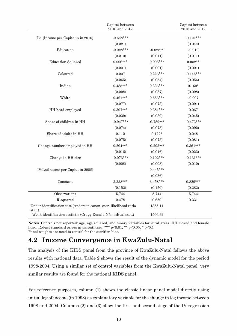
4.1 Income Convergence at National Level

Table 1presents the results for the classic linear panel model and the IV approach for the

period 2010-2012 in NIDS. The naïve estimation using the classic linear panel (Columns

1) with a standard set of control variables15 results in a highly significant and negative

impact of initial income of -0.548, implying a very strong convergence to the mean. When

allowing for measurement error (column 3), the coefficient of initial income drops from

-0.548 to -0.121, a reduction of 78%.16 In other words, for the national panel more than

three quarters of the obtained income convergence appears to be driven by measurement

error.

Robustness

To test for the robustness of these results with the national panel, the results from the two

instruments (i.e. Second lag income vs. Second lag of Asset index) are compared. The test

does not yield significant differences (see Table 3 below), which indicates that both

instruments are suitable to control for a similar level of measurement error. In addition,

the panel equation is again estimated using both instruments, which further corroborates

the results.17 The coefficient on the log of initial income in this case decreases to -0.161, a

reduction of 71% compared to the naïve estimator.

Overall, for both panel datasets indications for convergence to the mean are found. Income

mobility appears to be substantially overestimated when measurement error is not

controlled for. The magnitude of the measurement bias ranges between 71% and 78%in

the national NIDS panel.

Table 1: National Income Convergence (NIDS 2010-2012)

(1) (2) (3)

OLS IV

1st stage

IV

2nd stage

Outcome Change in log

(Income per

Ln(Income per

Capita, 2010)

Change in log

(Income per

15All control variables show the expected sign and are mostly highly significant. We find convex

returns to education, which is line with the South African literature (Keswell and Poswell, 2004).

Having a female household head or living in a big household seems to have a significant negative

income growth effect. As expected, being employed explains a large part of who is getting ahead or

falling behind. Income of black households seems to grow slower than Indian households. However,

the black coefficient turns insignificant for the IV regression. 16 All IV tests indicate that the Asset Index is an appropriate instrument. In addition an Asset

Index is used. Even when all (no) household characteristics are excluded and only (no) household

assets are used the coefficient for lagged income is relatively stable at the 10-20% level. This is true

for KIDS as well as for NIDS. 17 The over-identification test cannot be rejected, and other IV tests also hold, implying the validity

of the instrument set.

10

Capita) between

2010 and 2012

Capita) between

2010 and 2012

Ln (Income per Capita in in 2010) -0.548*** -0.121***

(0.021) (0.044)

Education -0.028*** -0.028** -0.012

(0.010) (0.011) (0.011)

Education Squared 0.006*** 0.005*** 0.002**

(0.001) (0.001) (0.001)

Coloured 0.007 0.226*** -0.145***

(0.065) (0.054) (0.056)

Indian 0.485*** 0.336*** 0.169*

(0.098) (0.087) (0.098)

White 0.461*** 0.556*** -0.007

(0.077) (0.073) (0.091)

HH head employed 0.307*** 0.381*** 0.067

(0.039) (0.039) (0.045)

Share of children in HH -0.947*** -0.789*** -0.473***

(0.074) (0.078) (0.092)

Share of adults in HH 0.112 0.122* 0.048

(0.075) (0.073) (0.081)

Change number employed in HH 0.204*** -0.293*** 0.361***

(0.016) (0.016) (0.023)

Change in HH size -0.073*** 0.102*** -0.131***

(0.008) (0.008) (0.010)

IV:Ln(Income per Capita in 2008) 0.445***

(0.036)

Constant 3.338*** 3.458*** 0.829***

(0.152) (0.150) (0.282)

Observations 5,744 5,744 5,744

R-squared 0.478 0.650 0.331

Under-identification test (Anderson canon. corr. likelihood ratio

stat.)

1385.11

Weak identification statistic (Cragg-Donald N*minEval stat.) 1566.39

Notes. Controls not reported: age, age squared, and binary variables for rural areas, HH moved and female

head. Robust standard errors in parentheses; *** p<0.01, ** p<0.05, * p<0.1

Panel weights are used to control for the attrition bias.

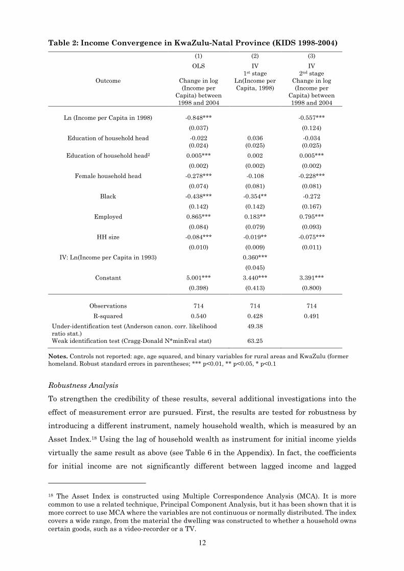
4.2 Income Convergence in KwaZulu-Natal

The analysis of the KIDS panel from the province of KwaZulu-Natal follows the above

results with national data. Table 2 shows the result of the dynamic model for the period

1998-2004. Using a similar set of control variables from the KwaZulu-Natal panel, very

similar results are found for the national KIDS panel.

For reference purposes, column (1) shows the classic linear panel model directly using

initial log of income (in 1998) as explanatory variable for the change in log income between

1998 and 2004. Columns (2) and (3) show the first and second stage of the IV regression

11

that allows for measurement error by instrumenting log of initial per capita income (in

1998) by the log of such income in 1993, the first wave of the data.

For the classic linear panel model the initial income variable is highly significant and has

a strong negative impact on income change. The outcome of this naïve estimator implies

that those with one unit higher log initial income in 1998 experience 84.8% lower log of

income change. That indicates a very strong conversion to the overall mean income, but

also confirms the findings of previous studies (e.g. Woolard and Klasen, 2005; Agüero et

al., 2007). However, using the IV approach results in a significantly lower coefficient,

which highlights the problem of measurement error and suggests that such error leads to

an overestimation of mobility and convergence. Since the time interval between the waves

is much shorter in the national data (only 2 years compared to 6 years in the KIDS data),

such a result would imply even faster income convergence at the national level.

The bias is smaller in the KIDS data from the KwaZulu-Natal province and ranges

between 33% and 44% of estimated income convergence. The preferred estimates using

two instruments suggest a bias in estimated income convergence by 77% for the NIDS panel

and 39% for the KIDS data.

Validity of IV Approach

Column (2) of the first stage shows that the instrument – the lag of ln(real per capita

income), i.e. the 1993 rather than 1998 values, from Wave 1 of KIDS – is highly significant.

Second, the Underidentification test (Anderson canon. corr. LM statistic), as well as the

Cragg-Donald statistic of the weak identification test, indicate that the instrument is

valid.

12

Table 2: Income Convergence in KwaZulu-Natal Province (KIDS 1998-2004)

(1) (2) (3)

OLS IV

1st stage

IV

2nd stage

Outcome Change in log

(Income per

Capita) between

1998 and 2004

Ln(Income per

Capita, 1998)

Change in log

(Income per

Capita) between

1998 and 2004

Ln (Income per Capita in 1998) -0.848*** -0.557***

(0.037) (0.124)

Education of household head -0.022 0.036 -0.034

(0.024) (0.025) (0.025)

Education of household head2 0.005*** 0.002 0.005***

(0.002) (0.002) (0.002)

Female household head -0.278*** -0.108 -0.228***

(0.074) (0.081) (0.081)

Black -0.438*** -0.354** -0.272

(0.142) (0.142) (0.167)

Employed 0.865*** 0.183** 0.795***

(0.084) (0.079) (0.093)

HH size -0.084*** -0.019** -0.075***

(0.010) (0.009) (0.011)

IV: Ln(Income per Capita in 1993) 0.360***

(0.045)

Constant 5.001*** 3.440*** 3.391***

(0.398) (0.413) (0.800)

Observations 714 714 714

R-squared 0.540 0.428 0.491

Under-identification test (Anderson canon. corr. likelihood

ratio stat.)

49.38

Weak identification test (Cragg-Donald N*minEval stat) 63.25

Notes. Controls not reported: age, age squared, and binary variables for rural areas and KwaZulu (former

homeland. Robust standard errors in parentheses; *** p<0.01, ** p<0.05, * p<0.1

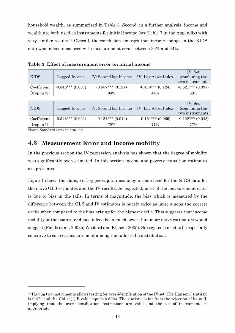
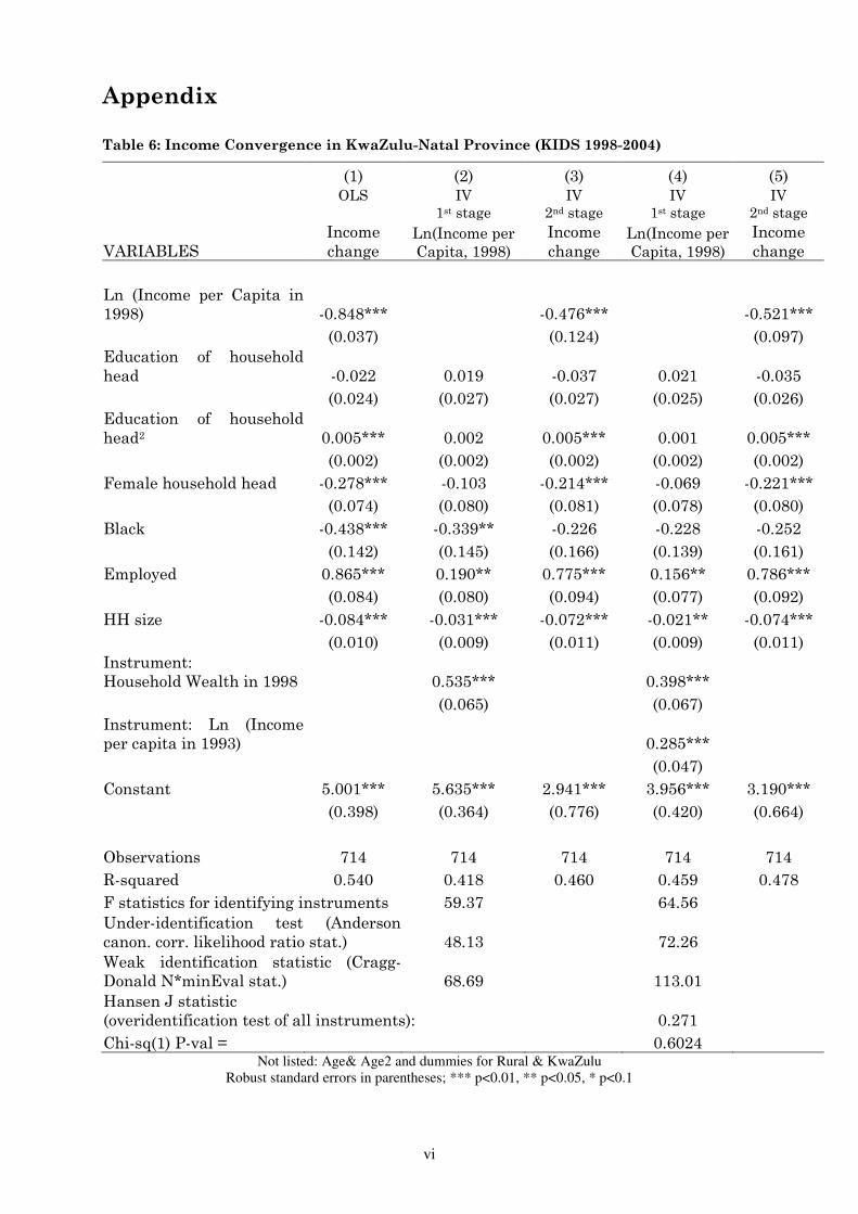
Robustness Analysis

To strengthen the credibility of these results, several additional investigations into the

effect of measurement error are pursued. First, the results are tested for robustness by

introducing a different instrument, namely household wealth, which is measured by an

Asset Index.18 Using the lag of household wealth as instrument for initial income yields

virtually the same result as above (see Table 6 in the Appendix). In fact, the coefficients

for initial income are not significantly different between lagged income and lagged

18 The Asset Index is constructed using Multiple Correspondence Analysis (MCA). It is more

common to use a related technique, Principal Component Analysis, but it has been shown that it is

more correct to use MCA where the variables are not continuous or normally distributed. The index

covers a wide range, from the material the dwelling was constructed to whether a household owns

certain goods, such as a video-recorder or a TV.

13

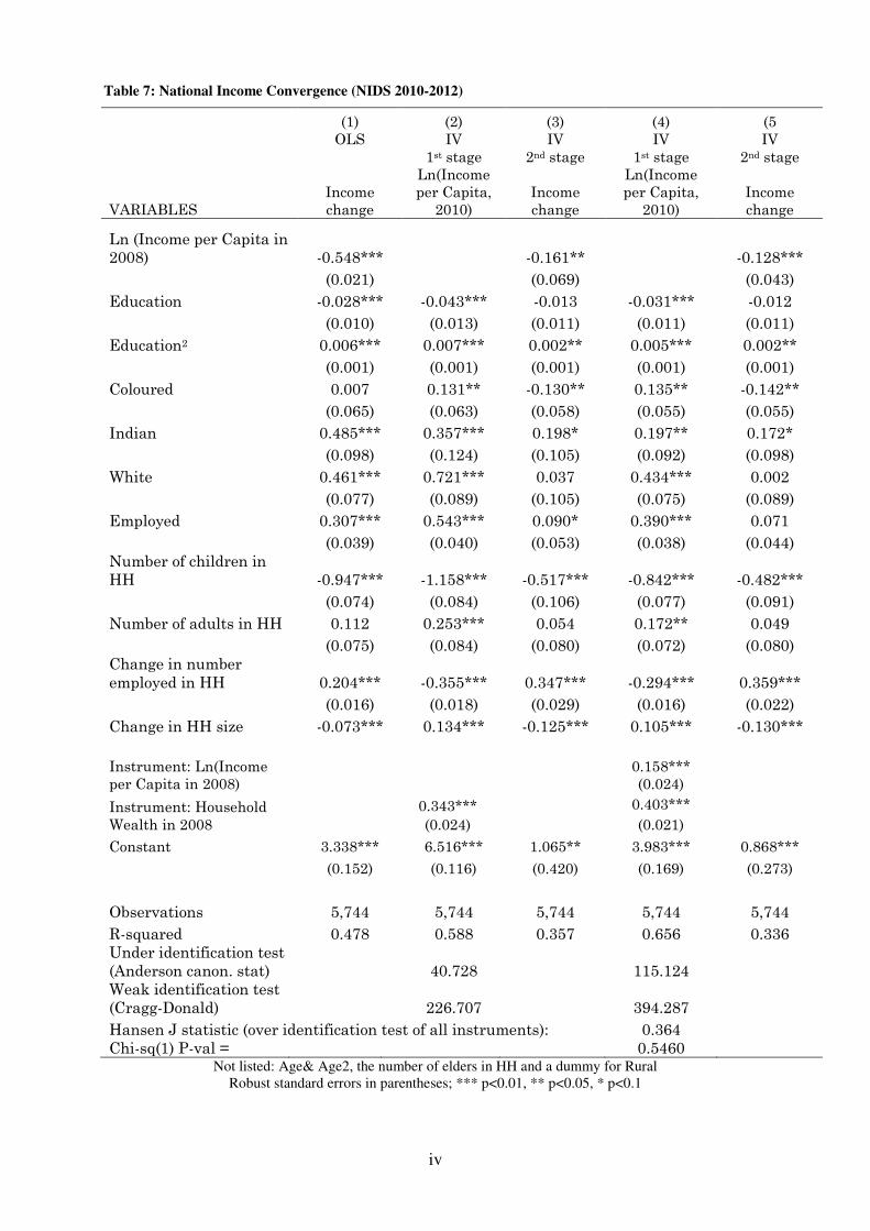
household wealth, as summarized in Table 3. Second, in a further analysis, income and

wealth are both used as instruments for initial income (see Table 7 in the Appendix) with

very similar results.19 Overall, the conclusion emerges that income change in the KIDS

data was indeed measured with measurement error between 34% and 44%.

Table 3: Effect of measurement error on initial income

KIDS Lagged Income IV: Second lag Income IV: Lag Asset Index

IV: Set

(combining the

two instruments

Coefficient -0.848*** (0.037) -0.557*** (0.124) -0.476*** (0.124) -0.521*** (0.097)

Drop in % 34% 44% 39%

NIDS Lagged Income IV: Second lag Income IV: Lag Asset Index

IV: Set

(combining the

two instruments

Coefficient -0.548*** (0.021) -0.121*** (0.044) -0.161*** (0.069) -0.128*** (0.043)

Drop in % 78% 71% 77%

Notes: Standard error in brackets

4.3 Measurement Error and Income mobility

In the previous section the IV regression analysis has shown that the degree of mobility

was significantly overestimated. In this section income and poverty transition estimates

are presented.

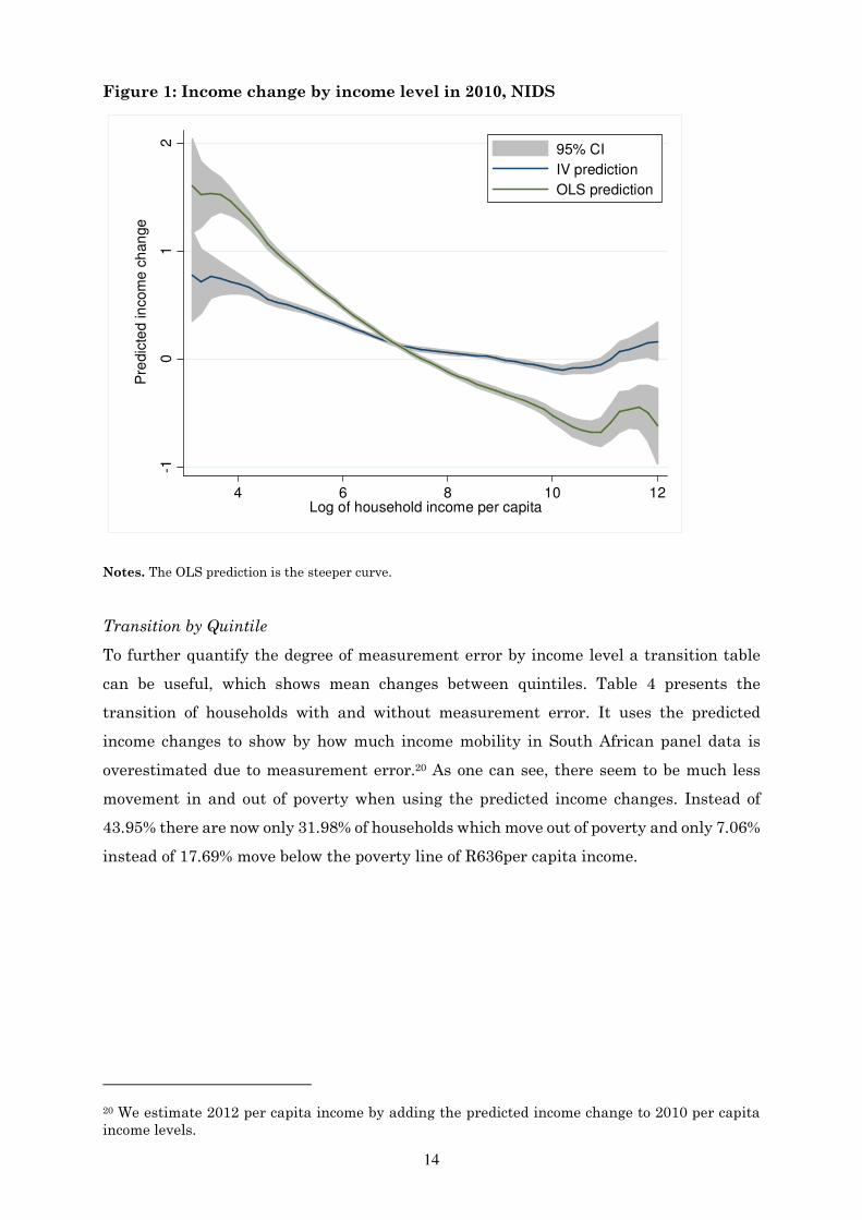
Figure1 shows the change of log per capita income by income level for the NIDS data for

the naive OLS estimates and the IV results. As expected, most of the measurement error

is due to bias in the tails. In terms of magnitude, the bias which is measured by the

difference between the OLS and IV estimates is nearly twice as large among the poorest

decile when compared to the bias arising for the highest decile. This suggests that income

mobility at the poorest end has indeed been much lower than more naive estimators would

suggest (Fields et al., 2003a; Woolard and Klasen, 2005). Survey tools need to be especially

sensitive to correct measurement among the tails of the distribution.

19 Having two instruments allows testing for over-identification of the IV set. The Hansen J statistic

is 0.271 and the Chi-sq(1) P-value equals 0.6024. The statistic is far from the rejection of its null,

implying that the over-identification restrictions are valid and the set of instruments is

appropriate.

14

Figure 1: Income change by income level in 2010, NIDS

Notes. The OLS prediction is the steeper curve.

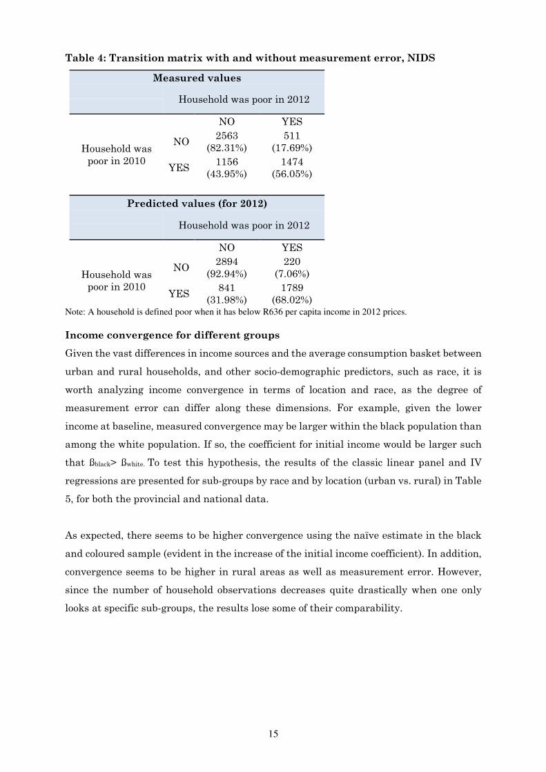
Transition by Quintile

To further quantify the degree of measurement error by income level a transition table

can be useful, which shows mean changes between quintiles. Table 4 presents the

transition of households with and without measurement error. It uses the predicted

income changes to show by how much income mobility in South African panel data is

overestimated due to measurement error.20 As one can see, there seem to be much less

movement in and out of poverty when using the predicted income changes. Instead of

43.95% there are now only 31.98% of households which move out of poverty and only 7.06%

instead of 17.69% move below the poverty line of R636per capita income.

20 We estimate 2012 per capita income by adding the predicted income change to 2010 per capita

income levels.

-10

12

Pre

dic

ted in

com

e c

han

ge

4 6 8 10 12Log of household income per capita

95% CI

IV prediction

OLS prediction

15

Table 4: Transition matrix with and without measurement error, NIDS

Measured values

Household was poor in 2012

NO YES

Household was

poor in 2010

NO 2563

(82.31%)

511

(17.69%)

YES 1156

(43.95%)

1474

(56.05%)

Predicted values (for 2012)

Household was poor in 2012

NO YES

Household was

poor in 2010

NO 2894

(92.94%)

220

(7.06%)

YES 841

(31.98%)

1789

(68.02%) Note: A household is defined poor when it has below R636 per capita income in 2012 prices.

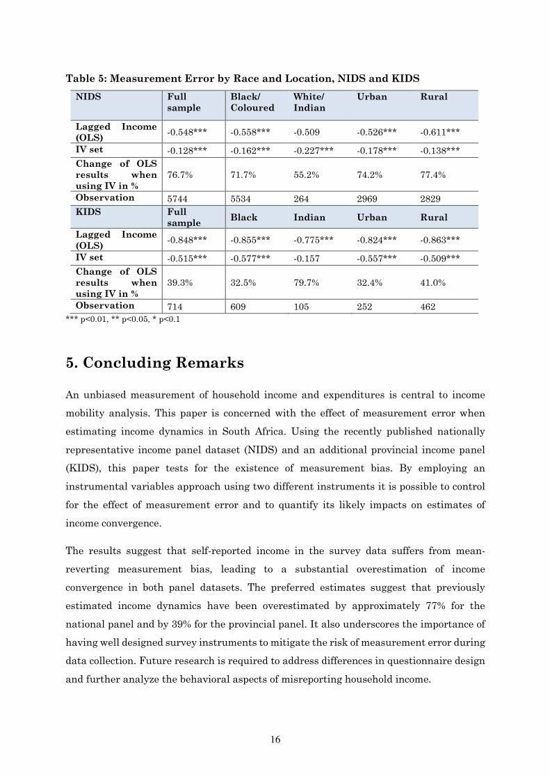
Income convergence for different groups

Given the vast differences in income sources and the average consumption basket between

urban and rural households, and other socio-demographic predictors, such as race, it is

worth analyzing income convergence in terms of location and race, as the degree of

measurement error can differ along these dimensions. For example, given the lower

income at baseline, measured convergence may be larger within the black population than

among the white population. If so, the coefficient for initial income would be larger such

that ßblack> ßwhite. To test this hypothesis, the results of the classic linear panel and IV

regressions are presented for sub-groups by race and by location (urban vs. rural) in Table

5, for both the provincial and national data.

As expected, there seems to be higher convergence using the naïve estimate in the black

and coloured sample (evident in the increase of the initial income coefficient). In addition,

convergence seems to be higher in rural areas as well as measurement error. However,

since the number of household observations decreases quite drastically when one only

looks at specific sub-groups, the results lose some of their comparability.

16

Table 5: Measurement Error by Race and Location, NIDS and KIDS

NIDS Full

sample

Black/

Coloured

White/

Indian

Urban Rural

Lagged Income

(OLS) -0.548*** -0.558*** -0.509 -0.526*** -0.611***

IV set -0.128*** -0.162*** -0.227*** -0.178*** -0.138***

Change of OLS

results when

using IV in %

76.7% 71.7% 55.2% 74.2% 77.4%

Observation 5744 5534 264 2969 2829

KIDS Full

sample Black Indian Urban Rural

Lagged Income

(OLS) -0.848*** -0.855*** -0.775*** -0.824*** -0.863***

IV set -0.515*** -0.577*** -0.157 -0.557*** -0.509***

Change of OLS

results when

using IV in %

39.3% 32.5% 79.7% 32.4% 41.0%

Observation 714 609 105 252 462

*** p<0.01, ** p<0.05, * p<0.1

5. Concluding Remarks

An unbiased measurement of household income and expenditures is central to income

mobility analysis. This paper is concerned with the effect of measurement error when

estimating income dynamics in South Africa. Using the recently published nationally

representative income panel dataset (NIDS) and an additional provincial income panel

(KIDS), this paper tests for the existence of measurement bias. By employing an

instrumental variables approach using two different instruments it is possible to control

for the effect of measurement error and to quantify its likely impacts on estimates of

income convergence.

The results suggest that self-reported income in the survey data suffers from mean-

reverting measurement bias, leading to a substantial overestimation of income

convergence in both panel datasets. The preferred estimates suggest that previously

estimated income dynamics have been overestimated by approximately 77% for the

national panel and by 39% for the provincial panel. It also underscores the importance of

having well designed survey instruments to mitigate the risk of measurement error during

data collection. Future research is required to address differences in questionnaire design

and further analyze the behavioral aspects of misreporting household income.

iv

References

Adato, M., M.R. Carter and J. May (2006), Exploring Poverty Traps and Social Exclusion

in South Africa using Qualitative and Quantitative Data, Journal of Development

Studies, 42 (2): 226–47.

Agüero, J., M. R. Carter and J. May (2007), Poverty and Inequality in the First Decade of

South Africa’s Democracy: What can be Learnt from Panel Data from KwaZulu-

Natal?, Journal of African Economies, Volume 16, Number 5, PP. 782–812.

Alexander, P., 2010. Rebellion of the poor: South Africa’s service delivery protests – a

preliminary analysis. Review of African Political Economy, 37, 25–40.

Antman, F. and D. J. McKenzie. Earnings mobility and measurement error: A pseudo-

panel approach. Vol. 3745. World Bank Publications, 2005.

Antman, F. and D. J. McKenzie (2007), Poverty traps and non-linear income dynamics

with measurement error and individual heterogeneity, Journal of Development

Studies, 43:6, 1057-1083.

Bhorat, H., P. Naidoo and C. van der Westhuizen (2006), Shifts in Non-income Welfare in

South Africa, 1993-2004, DPRU Conference Paper,18-20 October, Johannesburg.

Booysen, F., S. van der Berg, R. Burger, M. von Maltitz, and G. du Rand. (2008),Using an

Asset Index to Assess Trends in Poverty in Seven Sub-Saharan African Countries,

World Development, 36 (6), pp.1113–1130.

Carter, M. R. and May, J. (2001), One kind of freedom: poverty dynamics in post-apartheid

South Africa, World Development, 29(12), pp.1987–2006.

Dupas, P and J. Robinson (2012). The (hidden) costs of political instability: Evidence from

Kenya's 2007 election crisis, Journal of Development Economics, Vol 99(2), pp.314-

329.

Fields, G.S., Cichello, P., Freije, S., Menendez, M. and D. Newhouse, (2003a), For Richer

or for Poorer? Evidence from Indonesia, South Africa, Spain and Venezuela,

Journal of Economic Inequality 1(1), pp. 67–99.

Fields, G.D., Cichello, P., Freije, S., Menendez M. and D. Newhouse (2003b), Household

Income Dynamics: A Four Country Study, Journal of Development Studies 40(2),

pp.30–54.

Fields, G. S. (2008), A brief review of the literature on earnings mobility in developing

countries, working paper. Ithaca: Cornell University.

Fields, Gary S. and M. L. S. Puerta (2010), Earnings Mobility in Times of Growth and

Decline: Argentina from 1996 to 2003, World Development,38(6), pp.870-880.

Finn, A., Leibbrandt, M. and Levinsohn, J. (2013), `Income mobility in a high- inequality

society: Evidence from the National Income Dynamics Study', Development

Southern Africa 4(6).

Finn, A. and Leibbrandt, M. (2013). Mobility and Inequality in the First Three Waves of

NIDS. Cape Town: SALDRU, University of Cape Town. SALDRU Working Paper

Number 120/ NIDS Discussion Paper 2013/2.

Leibbrandt, M. et al. (2010), Trends in South African Income Distribution and Poverty

since the Fall of Apartheid, OECD Social, Employment and Migration Working

Papers, No. 101, OECD Publishing.

v

May, J., et al. (2000), KwaZulu-Natal Income Dynamics Study (KIDS) 1993-1998: A

longitudinal household data set for South African policy analysis, Development

Southern Africa, 17(4), pp. 567-581.

May, J., J. Agüero, M. R. Carter, and I. M. Timaeus (2007), The KwaZulu-Natal Income

Dynamics Study (KIDS) 3rd wave: methods, first findings and an agenda for future

research, Development Southern Africa, 24, pp. 629-648.

Keswell, M. and L. Poswell (2004), Returns to education in South Africa: A retrospective

sensitivity analysis of the available evidence, South African Journal of Economics,

72 (4), pp. 834–860.

Klasen, S. and I. Woolard (2008), Surviving Unemployment without State Support:

Unemployment and Household Formation in South Africa, Journal of African

Economies.

Schlemmer, L. (2005). Lost in Transformation? South Africa's Emerging Middle Class.

Centre for Development and Enterprise. CDE Focus Occasional Paper No 8

Van der Berg, S., M. Louw and D. Yu (2008), Post-transition Poverty Trends based on an

Alternative Data Source, South African Journal of Economics, 76(1), pp. 58-76.

Woolard,I. and S. Klasen (2005), Determinants of Income Mobility and Household Poverty

Dynamics in South Africa, Journal of Development Studies, 41(5), pp. 865-897.

Wooldridge, J. M.(2002), Econometrics Analysis of Cross Section and Panel

Data,Cambridge, MA: MIT Press.

vi

Appendix

Table 6: Income Convergence in KwaZulu-Natal Province (KIDS 1998-2004)

(1) (2) (3) (4) (5)

OLS IV

1st stage

IV

2nd stage

IV

1st stage

IV

2nd stage

VARIABLES

Income

change Ln(Income per

Capita, 1998)

Income

change Ln(Income per

Capita, 1998)

Income

change

Ln (Income per Capita in

1998) -0.848*** -0.476*** -0.521***

(0.037) (0.124) (0.097)

Education of household

head -0.022 0.019 -0.037 0.021 -0.035

(0.024) (0.027) (0.027) (0.025) (0.026)

Education of household

head2 0.005*** 0.002 0.005*** 0.001 0.005***

(0.002) (0.002) (0.002) (0.002) (0.002)

Female household head -0.278*** -0.103 -0.214*** -0.069 -0.221***

(0.074) (0.080) (0.081) (0.078) (0.080)

Black -0.438*** -0.339** -0.226 -0.228 -0.252

(0.142) (0.145) (0.166) (0.139) (0.161)

Employed 0.865*** 0.190** 0.775*** 0.156** 0.786***

(0.084) (0.080) (0.094) (0.077) (0.092)

HH size -0.084*** -0.031*** -0.072*** -0.021** -0.074***

(0.010) (0.009) (0.011) (0.009) (0.011)

Instrument:

Household Wealth in 1998 0.535*** 0.398***

(0.065) (0.067)

Instrument: Ln (Income

per capita in 1993) 0.285***

(0.047)

Constant 5.001*** 5.635*** 2.941*** 3.956*** 3.190***

(0.398) (0.364) (0.776) (0.420) (0.664)

Observations 714 714 714 714 714

R-squared 0.540 0.418 0.460 0.459 0.478

F statistics for identifying instruments 59.37 64.56

Under-identification test (Anderson

canon. corr. likelihood ratio stat.) 48.13 72.26

Weak identification statistic (Cragg-

Donald N*minEval stat.) 68.69 113.01

Hansen J statistic

(overidentification test of all instruments): 0.271

Chi-sq(1) P-val = 0.6024 Not listed: Age& Age2 and dummies for Rural & KwaZulu

Robust standard errors in parentheses; *** p<0.01, ** p<0.05, * p<0.1

iv

Table 7: National Income Convergence (NIDS 2010-2012)

(1) (2) (3) (4) (5

OLS IV

1st stage

IV

2nd stage

IV

1st stage

IV

2nd stage

VARIABLES

Income

change

Ln(Income

per Capita,

2010)

Income

change

Ln(Income

per Capita,

2010)

Income

change

Ln (Income per Capita in

2008) -0.548*** -0.161** -0.128***

(0.021) (0.069) (0.043)

Education -0.028*** -0.043*** -0.013 -0.031*** -0.012

(0.010) (0.013) (0.011) (0.011) (0.011)

Education2 0.006*** 0.007*** 0.002** 0.005*** 0.002**

(0.001) (0.001) (0.001) (0.001) (0.001)

Coloured 0.007 0.131** -0.130** 0.135** -0.142**

(0.065) (0.063) (0.058) (0.055) (0.055)

Indian 0.485*** 0.357*** 0.198* 0.197** 0.172*

(0.098) (0.124) (0.105) (0.092) (0.098)

White 0.461*** 0.721*** 0.037 0.434*** 0.002

(0.077) (0.089) (0.105) (0.075) (0.089)

Employed 0.307*** 0.543*** 0.090* 0.390*** 0.071

(0.039) (0.040) (0.053) (0.038) (0.044)

Number of children in

HH -0.947*** -1.158*** -0.517*** -0.842*** -0.482***

(0.074) (0.084) (0.106) (0.077) (0.091)

Number of adults in HH 0.112 0.253*** 0.054 0.172** 0.049

(0.075) (0.084) (0.080) (0.072) (0.080)

Change in number

employed in HH 0.204*** -0.355*** 0.347*** -0.294*** 0.359***

(0.016) (0.018) (0.029) (0.016) (0.022)

Change in HH size -0.073*** 0.134*** -0.125*** 0.105*** -0.130***

Instrument: Ln(Income

per Capita in 2008)

0.158***

(0.024)

Instrument: Household

Wealth in 2008

0.343***

(0.024)

0.403***

(0.021)

Constant 3.338*** 6.516*** 1.065** 3.983*** 0.868***

(0.152) (0.116) (0.420) (0.169) (0.273)

Observations 5,744 5,744 5,744 5,744 5,744

R-squared 0.478 0.588 0.357 0.656 0.336

Under identification test

(Anderson canon. stat) 40.728 115.124

Weak identification test

(Cragg-Donald) 226.707 394.287

Hansen J statistic (over identification test of all instruments): 0.364

Chi-sq(1) P-val = 0.5460 Not listed: Age& Age2, the number of elders in HH and a dummy for Rural

Robust standard errors in parentheses; *** p<0.01, ** p<0.05, * p<0.1