3. Nonparametric Regression

The multiple linear regression model is

Y = β0 + β1X1 + . . .+ βpXp + ε

where IE[ε] = 0, Var [ε] = σ2, and ε is independent of x1, . . . , xp.

The model is useful because:

• it is interpretable—the effect of each explanatory variable is captured by a single

coefficient

• theory supports inference and prediction is easy

• simple interactions and transformations are easy

• dummy variables allow use of categorical information

• computation is fast.

1

3.1 Additive Models

But additive linear fits are too flat. And the class of all possible smooths is too

large—the COD makes it hard to smooth in high dimensions. The class of additive

models is a useful compromise.

The additive model is

Y = β0 +

p∑

k=1

fk(xk) + ε

where the fk are unknown smooth functions fit from the data.

The basic assumptions are as before, except we must add IE[fk(Xk)] = 0 in order to

prevent identifiability problems.

The parameters in the additive model are {fk}, β0, and σ2. In the linear model, each

parameter that is fit costs one degree of freedom, but fitting the functions costs more,

depending upon what kind of univariate smoother is used.

2

Some notes:

• one can require that some of the fk be linear or monotone;

• one can include some low-dimensional smooths, such as f(X1, X2);

• one can include some kinds of interactions, such as f(X1X2);

• transformation of variables is done automatically;

• many regression diagnostics, such as Cook’s distance, generalize to additive

models;

• ideas from weighted regression generalize to handle heteroscedasticity;

• approximate deviance tests for comparing nested additive models are avaialable;

• one can use the bootstrap to set pointwise confidence bands on the fk (if these

include the zero function, omit the term);

However, model selection, overfitting, and multicollinearity (concurvity) are serious

problems. And the final fit may still be poor.

3

3.1.1 The Backfitting Algorithm

The backfitting algorithm is used to fit additive models. It allows one to use an

arbitrary smoother (e.g., spline, Loess, kernel) to estimate the {fk}

As motivation, suppose that the additive model is exactly correct. The for all

k = 1, . . . , p,

IE[Y − β0 −∑

k 6=j

fk(Xk) |xj ] = fj(xj).

The backfitting algorithm solves these p estimating equations iteratively. At

each stage it replaces the conditional expectation of the partial residuals, i.e.,

Y − β0 −∑

k 6=j fk(Xk) with a univariate smooth.

Notation: Let y be the vector of responses, let X be the n× p matrix of explanatory

values with columns x·k. Let fk be the vector whose ith entry is fk(xik) for

i = 1, . . . , n.

4

For z ∈ IRn, let S(z |x·k) be a smooth of the scatterplot of z against the values of the

kth explanatory variable.

The backfitting algorithm works as follows:

1. Initialize. Set β0 = Y and set the fk functions to be something reasonable (e.g., a

linear regression). Set the fk vectors to match.

2. Cycle. For j = 1, . . . , p set

fk = S(Y − β0 −∑

k 6=j

fk |x·k)

and update the fk to match.

3. Iterate. Repeat step (2) until the changes in the fk between iterations is

sufficiently small.

One may use different smoothers for different variables, or bivariate smoothers for

predesignated pairs of explanatory variables.

5

The estimating equations that are the basis for the backfitting algorithm have the

form:

Pf = QY

for suitable matrices P and Q.

The iterative solution for this has the structure of a Gauss-Seidel algorithm for linear

systems (cf. Hastie and Tibshirani; 1990, Generalized Additive Models, chap. 5.2).

This structure ensures that the backfitting algorithm converges for smoothers that

correspond to a symmetric smoothing matrix with all eigenvalues in (0, 1). This

includes smoothing splines and most kernel smoothers, but not Loess.

If it converges, the solution is unique unless there is concurvity. In that case, the

solution depends upon the initial conditions.

6

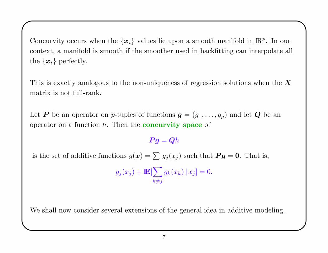
Concurvity occurs when the {xi} values lie upon a smooth manifold in IRp. In our

context, a manifold is smooth if the smoother used in backfitting can interpolate all

the {xi} perfectly.

This is exactly analogous to the non-uniqueness of regression solutions when the X

matrix is not full-rank.

Let P be an operator on p-tuples of functions g = (g1, . . . , gp) and let Q be an

operator on a function h. Then the concurvity space of

Pg = Qh

is the set of additive functions g(x) =∑

gj(xj) such that Pg = 0. That is,

gj(xj) + IE[∑

k 6=j

gk(xk) |xj ] = 0.

We shall now consider several extensions of the general idea in additive modeling.

7

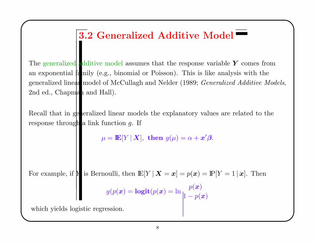
3.2 Generalized Additive Model

The generalized additive model assumes that the response variable Y comes from

an exponential family (e.g., binomial or Poisson). This is like analysis with the

generalized linear model of McCullagh and Nelder (1989; Generalized Additive Models,

2nd ed., Chapman and Hall).

Recall that in generalized linear models the explanatory values are related to the

response through a link function g. If

µ = IE[Y |X], then g(µ) = α+ x′β.

For example, if Y is Bernoulli, then IE[Y |X = x] = p(x) = IP[Y = 1 |x]. Then

g(p(x) = logit(p(x) = lnp(x)

1 − p(x)

which yields logistic regression.

8

The generalized additive model expresses the link function as an additive, rather than

linear, function of x:

g(µ) = β0 +

p∑

j=1

fj(xj).

As before, the link function is chosen by the user based on domain knowledge. Only

the relation to the explanatory variables is modeled.

Thus an additive version of logistic regression is

logit(p(x)) = β0 +

p∑

j=1

fj(xj).

Generalized linear models are fit by iterative scoring, a form of iteratively reweighted

least squares. The generalized additive model modifies backfitting in a similar way

(cf. Hastie and Tibshirani; 1990, Generalized Additive Models, chap. 6).

9

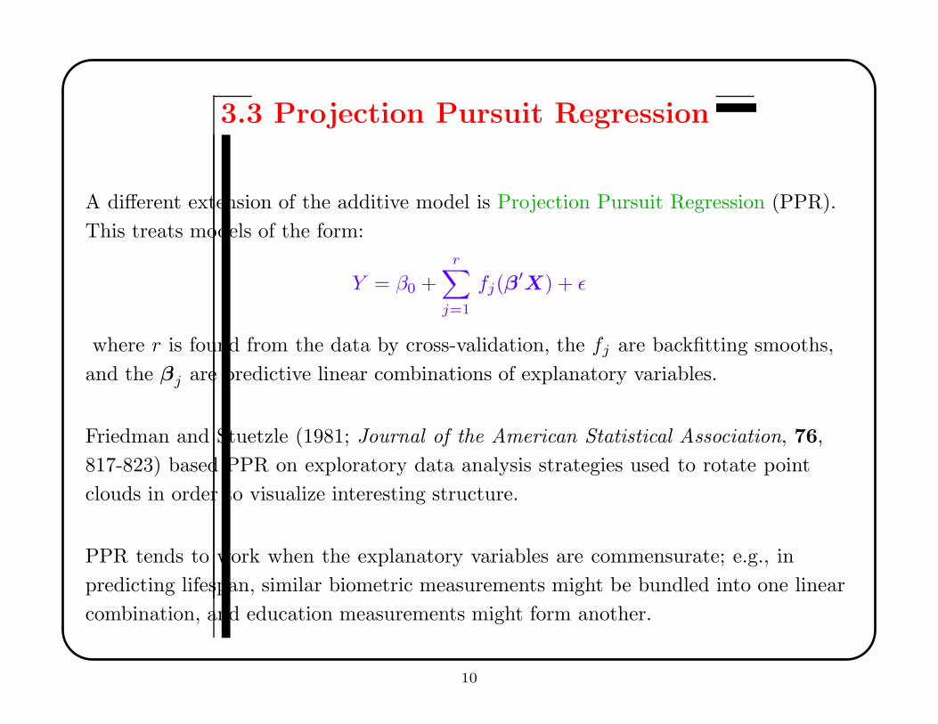
3.3 Projection Pursuit Regression

A different extension of the additive model is Projection Pursuit Regression (PPR).

This treats models of the form:

Y = β0 +r

∑

j=1

fj(β′X) + ε

where r is found from the data by cross-validation, the fj are backfitting smooths,

and the βj are predictive linear combinations of explanatory variables.

Friedman and Stuetzle (1981; Journal of the American Statistical Association, 76,

817-823) based PPR on exploratory data analysis strategies used to rotate point

clouds in order to visualize interesting structure.

PPR tends to work when the explanatory variables are commensurate; e.g., in

predicting lifespan, similar biometric measurements might be bundled into one linear

combination, and education measurements might form another.

10

Picking out a linear combination is equivalent to choosing a one-dimensional

projection of X. For example, take β′ = (1, 1) and x ∈ IR2. The β′x is the projection

of x onto the subspace S = {x : x1 = x2}.

11

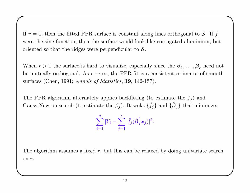
If r = 1, then the fitted PPR surface is constant along lines orthogonal to S. If f1

were the sine function, then the surface would look like corrugated aluminium, but

oriented so that the ridges were perpendicular to S.

When r > 1 the surface is hard to visualize, especially since the β1, . . . ,βr need not

be mutually orthogonal. As r → ∞, the PPR fit is a consistent estimator of smooth

surfaces (Chen, 1991; Annals of Statistics, 19, 142-157).

The PPR algorithm alternately applies backfitting (to estimate the fj) and

Gauss-Newton search (to estimate the βj). It seeks {fj} and {βj} that minimize:

n∑

i=1

[Yi −r

∑

j=1

fj(β′

jxj)]2.

The algorithm assumes a fixed r, but this can be relaxed by doing univariate search

on r.

12

The Gauss-Newton step starts with initial guesses for {fj} and {βj} and uses the

multivariate first-order Taylor expansion around the initial {βj} to improve the

estimated projection directions.

The PPR algorithm works as follows:

1. Fix r.

1. Initialize. Get initial estimates for {fj} and {βj}.

2. Loop.

For j = 1, . . . , r do:

fj(β′

jx) = S(Y −∑

j 6=k fk(β′

kx) |βj)

End For.

Find new βj by Gauss-Newton

If the maximum change in {βj} is less than some threshold, exit.

End Loop.

This converges uniquely under essentially the same conditions as for the AM.

13

3.4 Neural Networks

A third version of the additive model is neural networks. These methods are very

close to PPR.

There are many different fiddles on the neural network strategy. We focus on the

basic feed-forward network with one hidden layer.

14

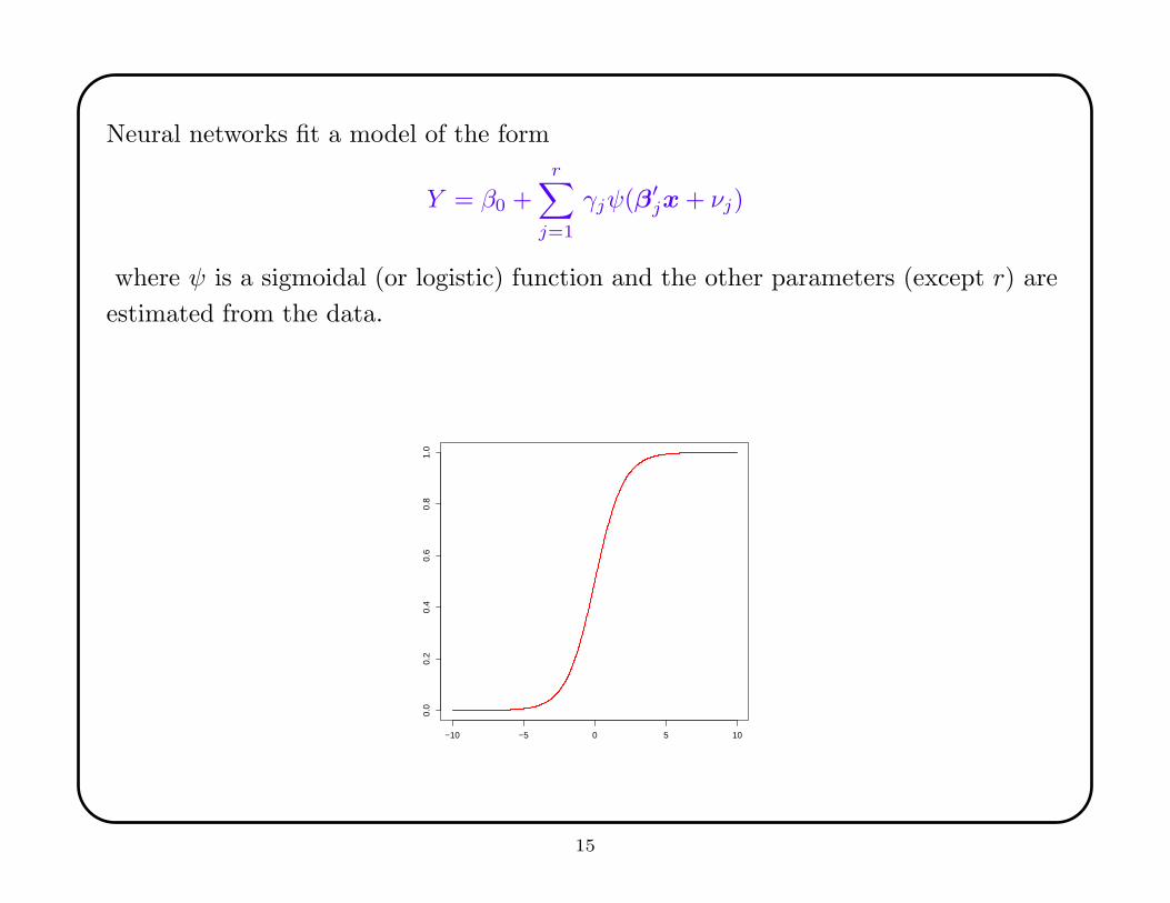
Neural networks fit a model of the form

Y = β0 +r

∑

j=1

γjψ(β′jx + νj)

where ψ is a sigmoidal (or logistic) function and the other parameters (except r) are

estimated from the data.

−10 −5 0 5 10

0.0

0.2

0.4

0.6

0.8

1.0

15

The only difference between PPR and the neural net is that neural nets assumes that

the additive functions have a parametric (logistic) form:

ψ(x) =1

1 + exp(α0 + β′x).

The parametric assumption allows neural nets to be trained by backpropagation, an

iterative fitting technique. This is very similar to backfitting, but somewhat faster

because it does not require smoothing.

Barron (1993; IEEE Transactions on Information Theory, 39, 930-945) showed that

neural networks evade the Curse of Dimensionality in specific, rather technical, sense.

We sketch his result.

16

A standard way of assessing the performance of a nonparametric regression procedure

is in terms of Mean Integrated Square Error (MISE). Let g(x) denote the true

function and g(x) denote the estimated function. Then

MISE[g] = IEF

[∫

[g(x) − g(x)]2 dx

]

where the expectation is taken with respect to the randomness in the data {(Yi,Xi)}.

Before Barron’s work, it had been thought that the COD implied that for any

regression procedure, the MISE had to grow faster than linearly in p, the dimension

of the data. Barron showed that neural networks could attain an MISE of order

O(r−1) + O(rp/n) lnn where r is the number of hidden nodes.

Recall that an = O(h(n)) means there exists c such that for n sufficiently large,

an ≤ ch(n).

17

Barron’s theorem is technical. It applies to the class of functions g ∈ Γc on IRp whose

Fourier transforms g(ω) satisfy∫

|ω|g(ω) dω ≤ c

where the integral is in the complex domain and | · | denotes the complex modulus.

The class Γc is thick, meaning that it cannot be parameterized by a finite-dimensional

parameter. But it excludes important functions such as hyperflats.

The strategy in Barron’s proof is:

• Show that for all g ∈ Γc, there exists a neural net approximation g∗ such that

‖g − g∗‖2 ≤ c∗/n.

• Show that the MISE in estimating any of the g∗ functions is bounded.

• Combine these results to obtain a bound on the MISE of a neural net estimate g

for an arbitrary g ∈ Γc.

18

3.5 ACE and AVAS

Alternating Conditional Expectations (ACE) seeks transformations f1, . . . , fp

and g of the p explanatory variables and the response variable Y that maximize the

correlation between

g(Y ) and

p∑

j=1

fj(Xj).

This is equivalent to minimizing

IE[(g(Y ) −

p∑

j=1

fj(Xj))2]/IE[g2(Y )]

where the expectations are taken with respect to {(Yi,Xi)}.

ACE modifies the additive modeling strategy by

• allowing arbitrary transformations of the response variable,

• using maximum correlation, squared error, for optimization.

19

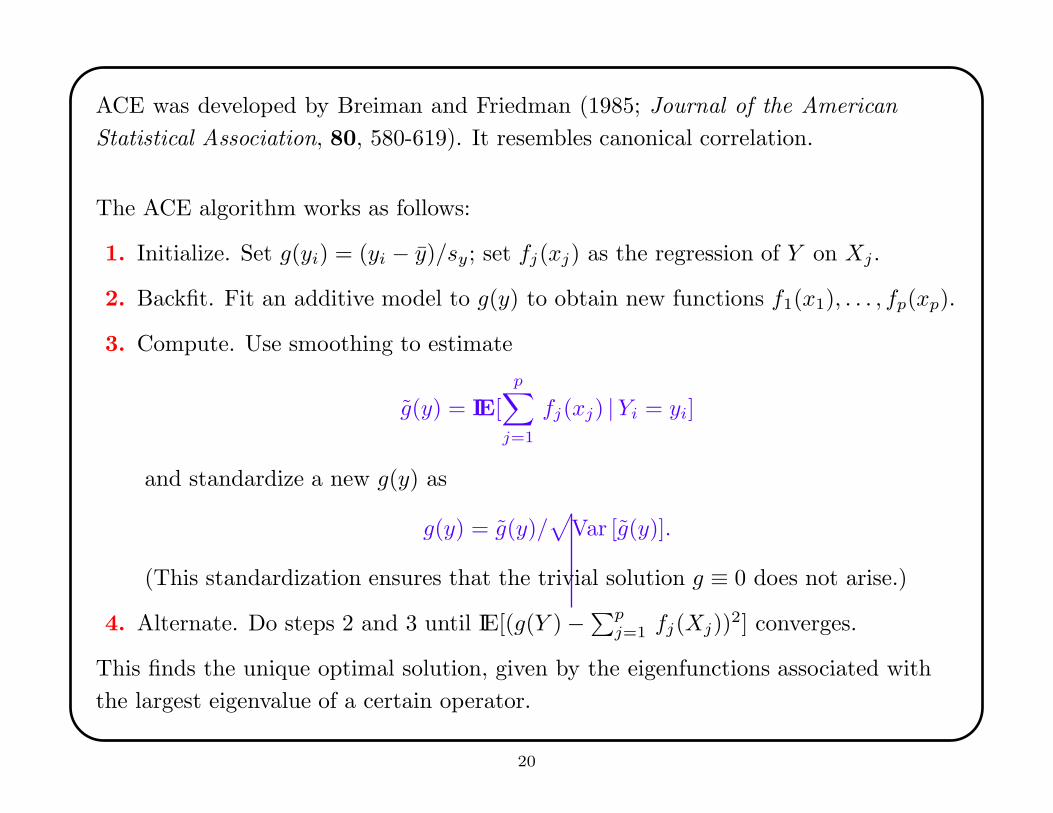
ACE was developed by Breiman and Friedman (1985; Journal of the American

Statistical Association, 80, 580-619). It resembles canonical correlation.

The ACE algorithm works as follows:

1. Initialize. Set g(yi) = (yi − y)/sy; set fj(xj) as the regression of Y on Xj .

2. Backfit. Fit an additive model to g(y) to obtain new functions f1(x1), . . . , fp(xp).

3. Compute. Use smoothing to estimate

g(y) = IE[

p∑

j=1

fj(xj) |Yi = yi]

and standardize a new g(y) as

g(y) = g(y)/√

Var [g(y)].

(This standardization ensures that the trivial solution g ≡ 0 does not arise.)

4. Alternate. Do steps 2 and 3 until IE[(g(Y ) −∑p

j=1 fj(Xj))2] converges.

This finds the unique optimal solution, given by the eigenfunctions associated with

the largest eigenvalue of a certain operator.

20

From the standpoint of nonparametric regression, ACE has several undersirable

features.

• If g(Y ) = f(X) + ε, then ACE generally will not find g and f but rather h ◦ g and

h ◦ f .

• The solution is sensitive to the marginal distributions of the explanatory variables.

• ACE treats the explanatory and response variables in the same way, but

regression should be asymmetric.

• The eigenfunctions for the second-largest eigenvalue can provide better insight on

the problem.

There are a few other pathologies. See the discussion of the Breiman and Friedman

article for additional examples and details.

21

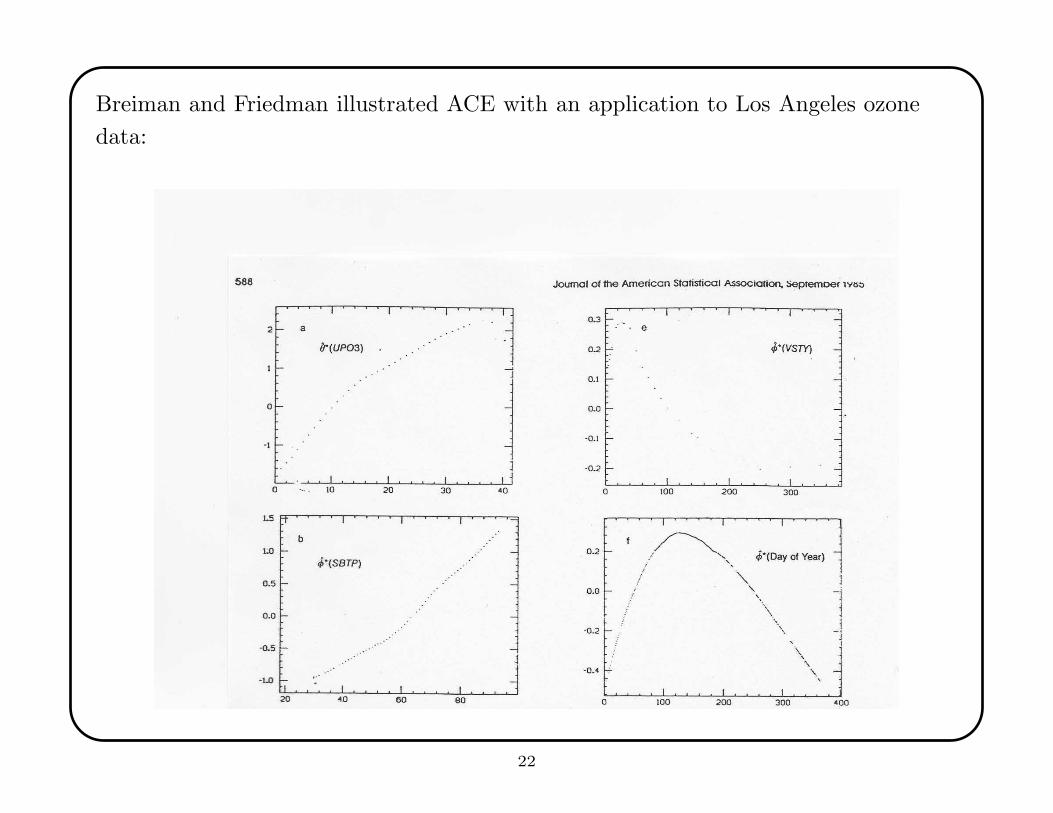
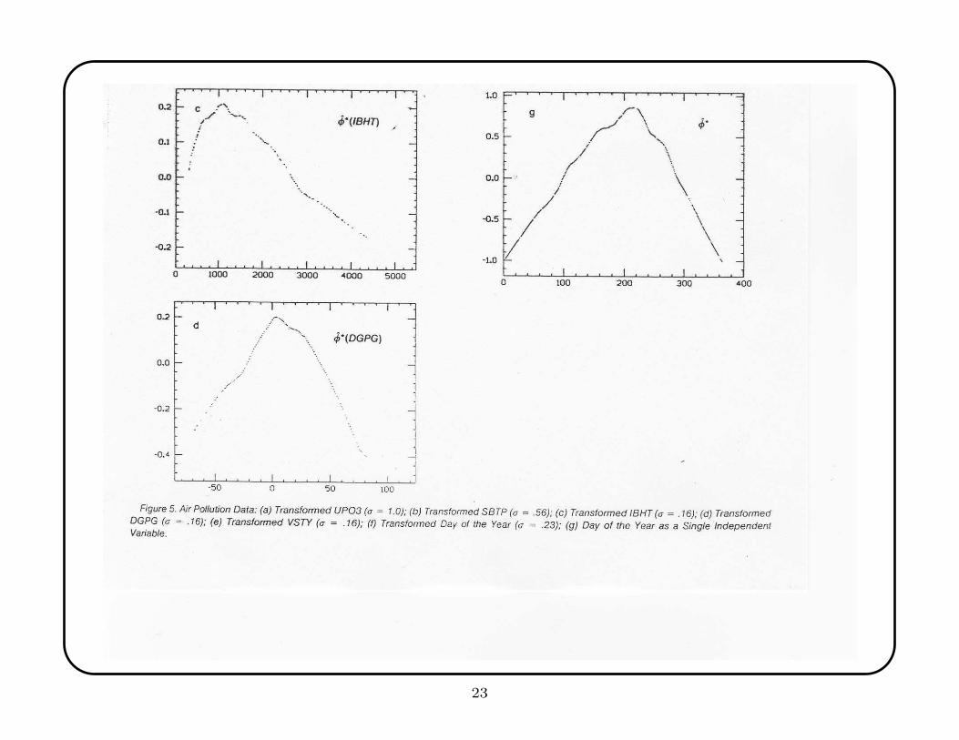
Breiman and Friedman illustrated ACE with an application to Los Angeles ozone

data:

22

23

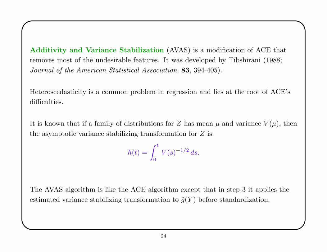
Additivity and Variance Stabilization (AVAS) is a modification of ACE that

removes most of the undesirable features. It was developed by Tibshirani (1988;

Journal of the American Statistical Association, 83, 394-405).

Heteroscedasticity is a common problem in regression and lies at the root of ACE’s

difficulties.

It is known that if a family of distributions for Z has mean µ and variance V (µ), then

the asymptotic variance stabilizing transformation for Z is

h(t) =

∫ t

0

V (s)−1/2 ds.

The AVAS algorithm is like the ACE algorithm except that in step 3 it applies the

estimated variance stabilizing transformation to g(Y ) before standardization.

24

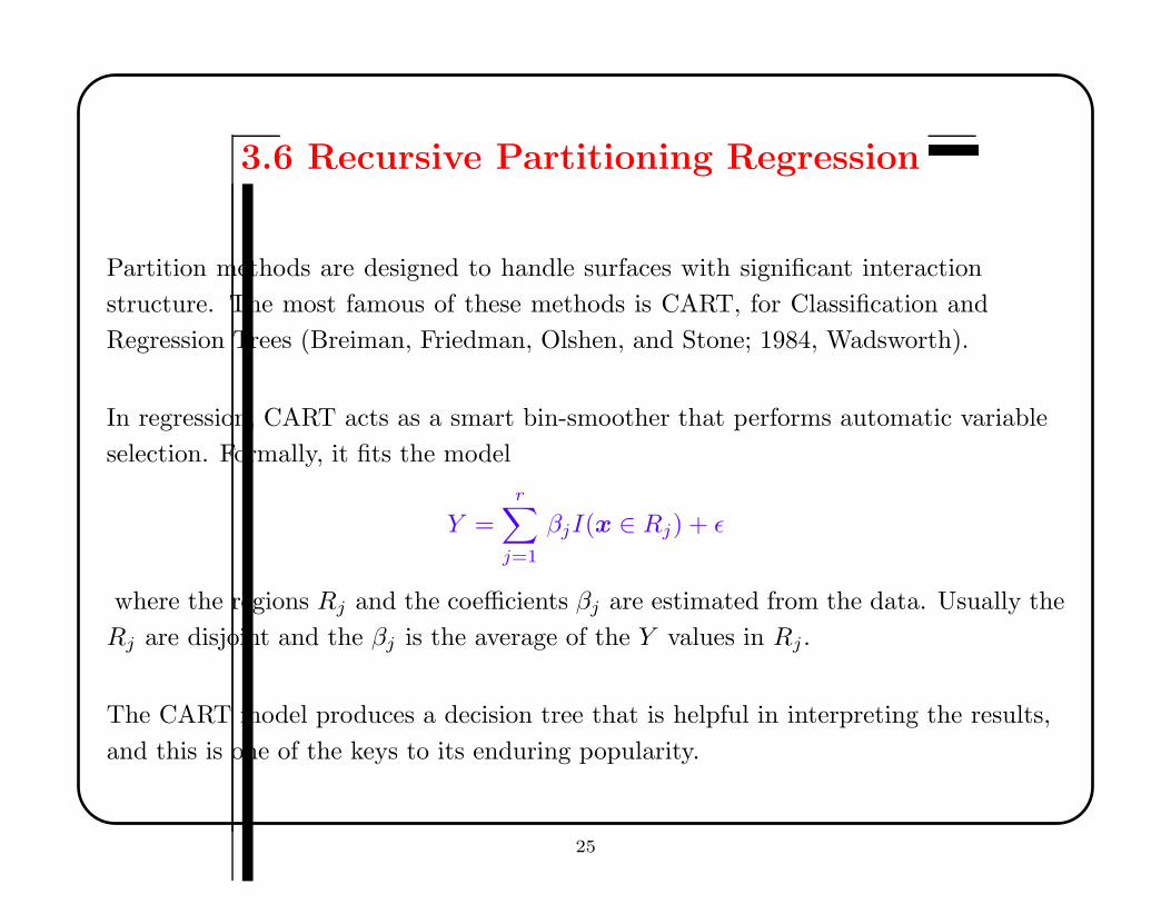
3.6 Recursive Partitioning Regression

Partition methods are designed to handle surfaces with significant interaction

structure. The most famous of these methods is CART, for Classification and

Regression Trees (Breiman, Friedman, Olshen, and Stone; 1984, Wadsworth).

In regression, CART acts as a smart bin-smoother that performs automatic variable

selection. Formally, it fits the model

Y =r

∑

j=1

βjI(x ∈ Rj) + ε

where the regions Rj and the coefficients βj are estimated from the data. Usually the

Rj are disjoint and the βj is the average of the Y values in Rj .

The CART model produces a decision tree that is helpful in interpreting the results,

and this is one of the keys to its enduring popularity.

25

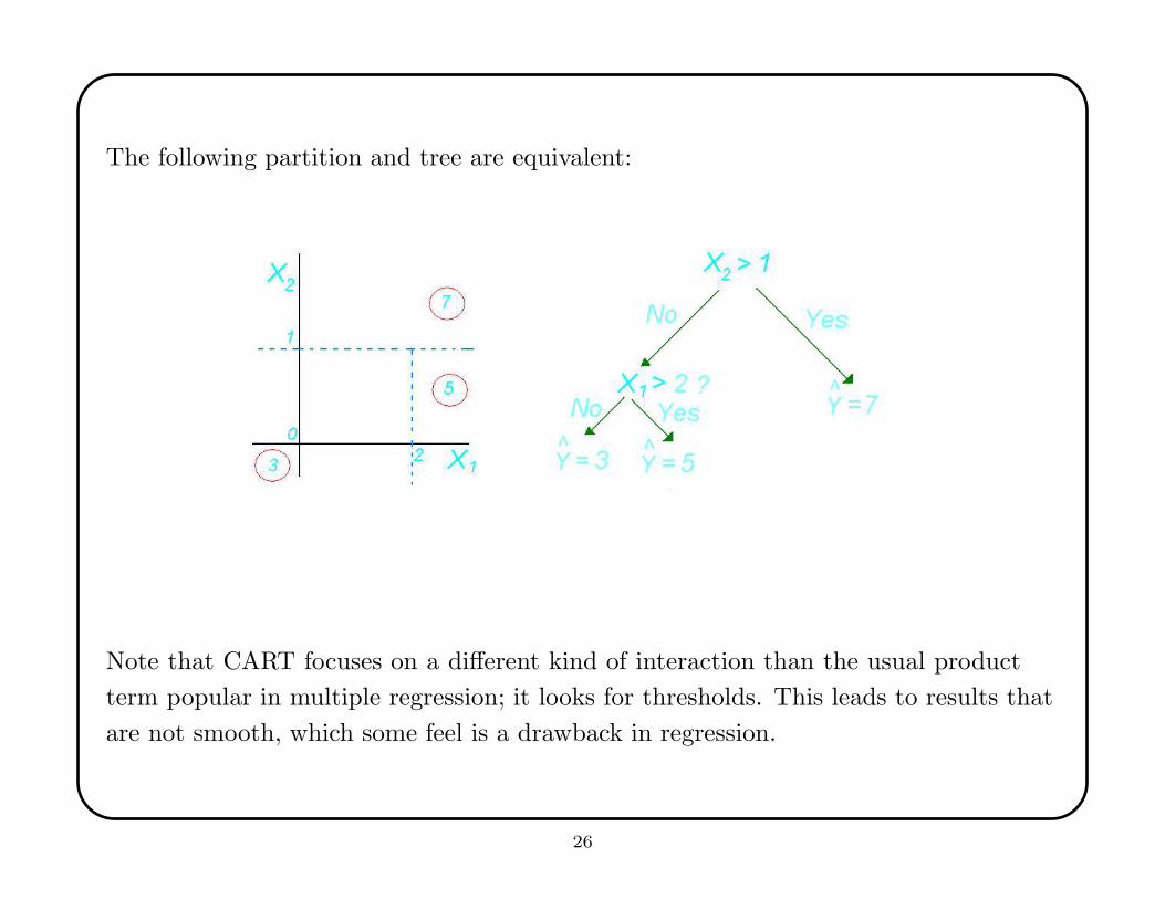
The following partition and tree are equivalent:

Note that CART focuses on a different kind of interaction than the usual product

term popular in multiple regression; it looks for thresholds. This leads to results that

are not smooth, which some feel is a drawback in regression.

26

The CART algorithm has three parts:

1. A way to select a split at each intermediate node.

2. A rule for declaring a node to be terminal.

3. A rule for estimating Y at a terminal node.

The third part is easy—just use the sample average of the cases at that terminal node.

The first part is also easy—split on the value x∗j which most reduces

SSerror =

n∑

i=1

(yi − fc(xi))2

Where fc is the predicted value from the current tree.

27

The second part is the hard one. One must grow an overly complicated tree, and then

use a pruning rule and cross-validation to find a tree with good predictive accuracy.

This entails a complexity penalty.

The main problems with CART are:

• discontinuous boundaries;

• it is difficult to approximate functions that are linear or additive in a small

number of variables;

• it is usually not competitive in low dimensions;

• one cannot tell when a complex CART model is close to a simple model.

The Boston housing data gives an example of the latter situation.

28

3.7 MARS

Multivariate Adaptive Regression Splines (MARS) improves on CART

by marrying it to PPR. It uses multivariate splines to let the data find flexible

partitions or IRp. And it incorporates PPR by letting the orientation of the region be

non-parallel to the natural axes.

The basic building block is a “hockeystick” (first-order truncated basis) function

(x− t)+, which looks like:

This is a special kind of tensor spline. It has a knot at t.

29

The fitted model has the form

Y =r

∑

j=1

βjBm(x) + ε

where

Bm(x) =∏

k∈K

[skm(xkm − tkm)]+

for skm = ±1 and K is a subset of the explanatory variables. Thus Bm is a product

of hockeysticks, so f is continuous. The regions are determined by the knots {tkm}.

The MARS algorithms starts with B1(x) = 1 and constructs new terms until there

are too many, as measured by generalized cross-validation.

Empirically, Friedman found that each term fit in a MARS model costs between 2

and 4 degrees of freedom. This reflects the variable selection involved in the fitting,

but not smoothing.

30

For each basis function Bm:

1. For all variables not in Bm,

A. try putting ± hockeysticks at every observation (candidate knot) in the

non-zero region of Bm;

B. select the best pair of hockeysticks according to an estimate of lack-of-fit.

2. Make two new basis functions from the product of Bm and the chosen pair of

hockeystick functions.

After building too many basis functions, prune back as in CART using

cross-validation.

Hockeysticks enter in pairs so that MARS is equivariant to sign changes.

Each Bm contains at most one term from each explanatory variable.

31

MARS is sort of interpretable, via an ANOVAesque decomposition:

f(x) = β0 +∑

j∈J

fj(xj) +∑

(j,k)∈K

fjk(xj , xk) + . . .

where β0 is the coefficient of the B1 basis function, the first sum is over those basis

functions that involve a single explanatory variable, the second sum is over those

basis functions that involve exactly two explanatory variables, and so forth.

These terms can be thought of as the grand mean, the main effects, the two-way

interactions, etc. One can plot these functions to gain insight.

MARS uses a tensor product basis (hence no explanatory variable appears twice in

any Bm). Additive effects are captured by splitting B1 on several variables. Nonlinear

effects are captured by splitting B1 with the same variable more than once.

32

MARS and CART are available commercially from Salford Systems, Inc., and versions

of them are available in S+ and R.

To get an integrated suite of code that that performs ACE, AVAS, MARS, PPR,

neural nets (the CASCOR version), recursive partitioning, and Loess, one can

download the DRAT package from

www.cs.cmu.edu/∼bobski/software/software.html

There are many kinds of neural network code. Users should be careful in using

it—there are many possible twiddles and performance may vary. CASCOR is due to

Fahlman and Lebiere (1990; Advances in Neural Information Processing Systems 2,

524-532, Morgan Kaufmann), and has the convenience of adaptively choosing the

number of hidden nodes.

33