1

3 realms ofgarch

modelling

Patrick Burns

Presented at the Imperial College Algorithmic Trading Conference on 2012 December 08.

http://www.icatg.com/#/algorithmic-trading-conference/4566871492

2

All models are wrong,some models are useful

– George Box

I think this is the most important slide in the talk.

Finance is particularly devoid of this knowledge.

The efficient market model is a prime example. Some people absolutely believe it. Some people absolutely don't believe it. The reality is that in some circumstances it is very useful. In other circumstances it is exceedingly dangerous.

The usefulness of a model has more to do with the use than the model.

3

Volatility clustering

Garch is a model. It models volatility clustering. There are periods of low volatility and periods of high volatility.

4

This is the daily returns of the S&P 500 over a few decades.

5

Finance

Statistics

Computing

Garch is impacted by these three fields. We'll see that there are problems in all three realms.

6

This is a picture of what garch thinks volatility looks like for the S&P 500. It is not actual volatility – we never get to see that – but we would have a hard time distinguishing real volatility from this picture.

7

garch mimics the mystery

There are some vague ideas floating around about why there is always volatility clustering in market data (“always” is a strong word, but I know of no counter-examples). At bottom, we don't know much about why volatility clustering exists.

Garch doesn't help us with that. It only mimics the phenomenon, it does not explain it.

8

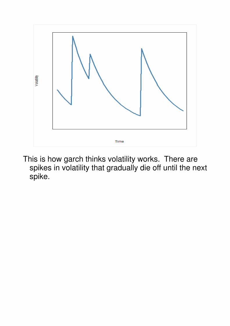
This is how garch thinks volatility works. There are spikes in volatility that gradually die off until the next spike.

9

garch says there arelarge spikes in volatilitythat gradually die off

Spikes are unpredictable

When the spikes happen is unpredictable.

Well, some people might think that they can predict the spikes. I'll be a bit dubious.

Most certainly, though, garch is NOT predicting the spikes. That's not what it does.

10

garch is magic

Garch is magic because it predicts something for us that we can never see (no visible rabbit).

There is a price for magic.

Picture by miamiamia via stock.xchng

11

garch is data hungry

In this case the price of magic is that garch really, really wants a lot of data.

Photo by patbain via stock.xchng

12

ht = ωωωω + αεαεαεαε

t-1

2 + ββββht-1

This is the equation for the garch(1,1) model.

ht is the conditional variance at time t. Conditional on

what has happened up to time t.

ω, α, β are parameters. We want our estimated variance to be positive, so we will constrain these parameters to be non-negative.

The best way to think of εt is that it is the return at

time t. It is really the return minus the expected value of the return at that time point. But up to an excellent approximation, it is the return.

13

ht = ωωωω + αεαεαεαε

t-1

2 + ββββht-1

Let's muck with the equation a little.

Set ω to zero and α to 1-β. Then we have an exponential smooth.

Suppose β is 0.97. Then 0.97 times today's variance plus 0.03 times today's squared return gives us tomorrow's variance.

One way to think about garch is that it is an exponential smooth in a fancy suit.

14

This is pretty picture #1.

We specify a specific set of parameters. Those

specifications include 0.07 for α and 0.925 for β.

We create (simulate) a dataset using the specific parameters. Then we fit the garch model on that dataset. The resulting estimates will, of course, not be exactly the true parameter values. We get one point on this plot.

Then we do that over and over to build up this cloud of points.

15

This is still pretty picture #1.

We see quite good estimation of the parameters in this plot. The range of the estimates is about 0.01 in both cases.

You're not going to get this sort of precision. The datasets for this plot each had 100,000 observations. If we are talking about daily data, that is a mere 4 centuries.

16

This is pretty picture #2.

Your results will be more like this, where there are 2000 observations. Estimates are not nearly so precise in this case.

The plot also has a weird cliff at the top, unlike the previous plot that was a smooth mound like we are used to. We'll see later why that cliff is there.

17

natural frequency Is daily

The nicest frequency for garch is daily.

Garch likes a lot of data, so weekly and monthly is not good.

We can get more observations by going intraday. But there is volatility seasonality through the day.

The canonical pattern is high volatility at the open and close and lower volatility in the middle of the day. But the pattern definitely depends on the market. It can depend on the asset, and it can change through time.

Intraday garch models are possible, but not simple.

18

garch has predictions

One of the key reasons that garch is useful is because we can get predictions with it.

19

hT+k+1

= ωωωω + αεαεαεαεT+k

2 + ββββhT+k

If we want to predict k+1 steps beyond our data, then we can just write down the equation and see what we need to do.

By this point we have already estimated ω, α and β.

We are going to do the estimation iteratively step by step. So if we can get anywhere, then h

T+k won't be

a problem.

There is a problem with ε2 k steps ahead. We don't know that. But we do know its expectation – that is the conditional variance at that point in time.

20

hT+k+1

= ωωωω + αεαεαεαεT+k

2 + ββββhT+k

hT+k+1

= ωωωω + ααααhT+k

+ ββββhT+k

Hence we get the bottom equation.

This shows us that α+β is something special for the garch(1,1) model.

21

hasym

= ωωωω + ααααhasym

+ ββββhasym

hasym

= ωωωω / (1 - αααα - β)β)β)β)

If we can predict out to infinity, then the top equation must be true. The top equation implies the second equation.

The bottom one makes sense when α+β is less than 1.

Looking at the second equation on the previous slide,

we see that if ω is positive and α+β is at least 1,

then we will go off to infinity. But if α+β is less than 1, we stay finite.

22

Halflife:

log(.5) / log(αααα + β)β)β)β)

One way to express the meaning of α+β is with the halflife.

23

Here is data that corresponds to pretty picture #2, where the datasets are 2000 long.

The true halflife is 138 days. A lot of the estimated halflives are less than 100. There is also a significant minority that are about 700, but then it stops. It stops because the fitting routine

constrains α+β to be (by default) less than .999, which corresponds to a halflife of 693.

That is why there is a cliff in pretty picture #2.

24

garch optimisation is hard

By now it shouldn't be surprising to hear that optimization of garch models is difficult.

We're estimating something that is unobservable. The variability of the estimates is very high.

So troublesome optimization just completes the set.

25

Garch thinks that volatility should look like this.

26

But it sees something like this.

It sees lots of noise. It is hard for it to see how fast the decay is and how high the spikes should jump.

27

garch optimization is hard

garch invented in the 80's

Garch started out in the 80's.

In the 80's and 90's computers weren't quite what they are now.

And optimization software wasn't quite then what it is now.

Fitting a garch model wasn't such a trivial task in the olden days before the web.

28

Variance targeting

hasym

= ωωωω / (1 - αααα - β)β)β)β)

This is why the idea of variance targeting was born.

We've seen this equation before, but let's think about

it from a computing point of view. α+β is close to 1

so ω is small. That means that small changes in these three parameters could have quite a big impact on the asymptotic variance.

But we have a pretty good estimate of the asymptotic variance – the unconditional variance of our dataset.

29

Variance targeting

hasym

= ωωωω / (1 - αααα - β)β)β)β)

The variance targeting plan is to fix the asymptotic variance. Then when the optimizer has selected an

α and β, we know what ω has to be.

So we are eliminating one parameter from the optimization. That's a good thing with slow computers and dodgy optimizers. Moreover, it is a very troublesome parameter.

The result was that optimizations were faster, and tended to get higher likelihoods.

That is wrong mathematically – imposing a constraint must have a lower maximum likelihood than without the constraint. But computationally it can (and did) happen.

30

What is the statistical impact of variance targeting with our modern, better (but not perfect) optimizers?

Here we see the mean squared error for the parameters compared with and without variance targeting. In all but one case variance targeting slightly degrades the parameter estimation.

This makes sense, we are paying a statistical price for a computing convenience.

In the olden days with poor optimizers, the variance targeting probably would have helped in all cases.

31

There are quantities that we care more about than the model parameters. If we look at halflife and asymptotic variance, it's a different picture.

If we have all the data we want, then imposing the targeting is a bad thing. The estimation can find its way better on its own.

But in the realistic case variance targeting helps. It is stabilizing us from the noise that is in the data.

32

At this point I did a demo of the 'rugarch' R package using Rstudio.

I did no more than two or three embarrassing things.

The audience forced me into learning something about the effect of parameters.

33

Better models

I would have liked to have shown them better models in R than the garch(1,1). There are other models in R. Maybe some of them are better.

34

Components model

I do know of a model that is definitely better than garch(1,1). It is called the components model.

35

ht = q

t + α(εα(εα(εα(ε

t-1

2 - qt-1

) + β(β(β(β(ht-1

- qt-1

)

qt = ωωωω + ρρρρq

t-1 + φφφφ(εεεε

t-1

2 - qt-1

)

The components model has this set of equations.

The way to think about it is that there is a smooth long-term trend in volatility and then short-term volatility wiggles around the long-term trend.

That is the way to think of it, but the reality is that the long-term trend is not smooth – it looks just as jagged as the volatility.

36

Better models

I said the components model is better.

What does better mean?

I think it has to mean better prediction and/or better simulation.

I'll only talk about prediction.

One of the goals of the demonstration was to suggest that small changes in parameter values are unlikely to have much effect on in-sample prediction. In-sample prediction is only predicting one step ahead.

37

Better models

We always have all the elements we need for one-step ahead prediction.

If we predict two steps ahead, then we need to start using the expectation of squared residuals. The more steps ahead we predict, the more we are dependent on our model being good.

A key part of predicting ahead is getting the rate of decay right.

38

We've seen this picture before. It is quite common for the halflife to be underestimated with the garch(1,1) model.

That means that predictions very quickly converge to the asymptotic variance.

39

ht = q

t + α(εα(εα(εα(ε

t-1

2 - qt-1

) + β(β(β(β(ht-1

- qt-1

)

qt = ωωωω + ρρρρq

t-1 + φφφφ(εεεε

t-1

2 - qt-1

)

The parameter ρ is the persistence in the

components model – it is equivalent to α+β in the garch(1,1).

The estimated persistence tends to be larger in the components model than in the garch(1,1) for the same data. The components model does a better job of getting the halflife right.

40

ht = q

t + α(εα(εα(εα(ε

t-1

2 - qt-1

) + β(β(β(β(ht-1

- qt-1

)

qt = ωωωω + ρρρρq

t-1 + φφφφ(εεεε

t-1

2 - qt-1

)

The components model has another trick up its sleeve.

It is possible to be in a high volatility long-term regime but low volatility short-term, and vice versa.

garch(1,1) predictions always go towards the asymptotic variance. If we start out above it, predictions always decrease. If we start out below it, predictions always increase.

In the components model predictions can go up and then down, or down and then up.

The components model does a better job of extracting information from the data about the current state of volatility.

41

Why isn't the components model

in R (and elsewhere)?

(I'm hoping that this slide will soon be obsolete.)

This seems like something that might be really mysterious, but the answer is quite clear.

The goal with the components model and the literally hundreds of other garch models that have been invented has been to publish a paper. There was very little emphasis on allowing people to actually use the model.

I think that emphasis might be beginning to change.

42

Your uniformly most

wonderful garch model

If you have a research project that is an idea for an absolutely wonderful garch model, you will need a computing environment. I have guesses for the three most likely environments that you will use.

Guess 1: Ox. The good thing about Ox is that people who use it love it. The bad thing about Ox is that as far as I know it is never ever used outside academia.

Guess 2: Matlab. The good thing about Matlab is that it is used in practice. I see two downsides to it: When you move institutions, you will need to pay to use your own software. There is not an established mechanism for sharing Matlab code.

43

Your uniformly most

wonderful garch model

Guess 3: R. The downside of R is that if you don't already know it, it may take you a while to get used to it. The two upsides are: It is used in practice, and that use seems to be increasing quite rapidly. There is both the infrastructure and the culture to share R code.

If you use R, it will be very easy for people to use your model.

If others also create models in R, then it will be easy for us as a community to test and compare the models.

We can advance faster if we select models scientifically rather than leaving the selection of the dominant model to chance and folklore.

44

Questions and (some) Answers

Robert Macrae asked a question the answer to which was that the hypothesized error distribution matters.

Assuming a t-distribution (and estimating the degrees of freedom) is definitely better than assuming a normal distribution.

I've tried other distributions as well in the past. The t seemed to be the best of those I tried.

This suggests that the default in software should be the t distribution and not the normal.