Structural GARCH: The Volatility-Leverage Connection⇤

(Preliminary and Incomplete)

Robert Engle† Emil Siriwardane‡

October 8, 2013

Abstract

We propose a new model of volatility where financial leverage amplifies equity volatility by what

we call the “leverage multiplier”. The exact specification is motivated by standard structural models of

credit; however, our parametrization departs from the classic Merton (1974) model and is, as we show,

flexible enough to capture environments where the firm’s asset volatility is stochastic and asset shocks

are non-normal. As a result, our model also provides estimates of asset returns and asset volatility. In

addition, our specification nests both a standard GARCH and the classical Merton model, which allows

for a simple statistical test of how leverage interacts with equity volatility. We then apply the Structural

GARCH model to two applications: the leverage effect and systemic risk measurement.

⇤We are grateful to Viral Acharya for valuable comments and discussions; and to seminar participants at NYU Stern. Wewould also like to thank Rob Capellini for all of his help on this project.

†Affiliation: NYU Stern School of Business. Address: 44 West 4th St., Floor 9-Room 197K. New York, NY 10012. E-mail:rengle@stern.nyu.edu

‡Affiliation: NYU Stern School of Business. Address: 44 West 4th St., Floor 9-Room 197K. New York, NY 10012. E-mail:esiriwar@stern.nyu.edu

1

1 Introduction

In the financial crisis of 2007-2009 it is widely observed that equity volatilities hit sustained levels not seen

since the Great Depression. This was particularly true for the financial sector. Yet it is also observed that

the leverage in the financial sector reached extremely high levels. When firm leverage is high, measured

by firm asset value divided by equity value, it is not surprising that equities would be highly volatile. Is

it possible that asset volatility did not rise during the financial crisis even though equity volatility hit such

high levels?

In this paper we propose an econometric approach to disentangle the effects of leverage on equity volatility.

The model is based on the classic Merton (1974) model of firm capital structure extended to incorporate

time variation in asset volatility. It is motivated by the Schaefer and Strebulaev (2008) finding that hedge

ratios from this model may be quite accurate even though the levels are not well determined. The empirical

results reveal that at the beginning of the financial crisis the rise in equity volatility is primarily due to rising

leverage but later phases also include substantial rises in asset volatility. The model additionally sheds light

on the well known asymmetry in volatility models and on the impact of debt maturities.

Section 2 introduces the Structural GARCH model and its economic underpinnings. Here, we will use

basic ideas from structural models of credit to explore the relationship between leverage and equity volatility,

which leads to a natural econometric specification for equity and asset returns. In Section 3, we describe

the data we use in our empirical work, along with some technical issues regarding estimation of the model.

Section 4 describes our empirical results and explores some aggregate implications of our model. In Section

5, we apply the Structural GARCH model to two applications: asymmetric volatility in equity returns, and

systemic risk measurement. Finally, Section 6 concludes and suggests extensions of the baseline Structural

GARCH model.

2 Structural GARCH

Our goal is to explore the relationship between the leverage of a firm and its equity volatility. A simple

framework to explore this relationship is through the classical Merton (1974) model of credit risk. Equity

holders are entitled to the assets of the firm that exceed the outstanding debt. As Merton observed, equity

can then be viewed as a call option on the total assets of a firm with the strike of the option being the debt

2

level of the firm. In this model, the fact that firms have outstanding debt of varying maturities is ignored,

which we will entertain for the sake of maintaining a simple econometric model. The purpose of using the

Merton model is to provide economic intuition for how leverage and equity volatility should interact.

2.1 Motivating the Model

As is standard in structural models of credit, the equity value of a firm is function of the asset process and

the debt level of the firm. We can therefore define the equity value as follows:

Et = f⇣At, Dt,�

fA,t, ⌧, rt

⌘

= Dt ⇥ f⇣At/Dt, 1,�

fA,t, ⌧, rt

⌘(1)

where f(·) is an unspecified call option function, At is the current market value of assets, Dt is the current

book value of outstanding debt, �fA,t is the volatility of the assets over the life of the debt, ⌧ is the life of the

debt, and finally rt is the annualized risk-free rate at time t. The second line of the Equation (1) assumes

that the call option function is homogenous of degree one in its first two arguments, which is a standard

assumption in the option pricing literature. Moreover, in order for the relationship in Equation (1) to hold

true in a general sense, we assume that the future distribution of volatility is unimportant for the option

value. As we will see, our volatility model is flexible enough that this is not a restrictive assumption. The

instantaneous return on equity is computed via simple differentiation:

dEt

Et= �t ·

At

Dt· Dt

Et· dAt

At+

@f

@�fA,t

· Dt

Et· d�f

A,t (2)

where �t = @f⇣At/Dt, 1,�

fA,t, ⌧, r

⌘/@At is the familiar “delta” in option pricing. Here, we have ignored the

sensitivity of the option value to the maturity of the debt. In our applications, ⌧ will be large enough that

this assumption is innocuous. In the Online Appendix, we show that the last terms of Equation (2) is small

in magnitude relative to the first term for the purposes of volatility modeling, and thus can be ignored in

our applications.1

In reality, we do not observe At as it is the market value of assets. However, given that the call option1Intuitively, forecast volatility over longer horizons will be virtually constant because volatility mean reverts relatively quickly.

In addition, we estimate a model where we enforce a constant �fA,t.

3

pricing function is monotonically increasing in its first argument, it is safe to assume that f(·) is invertible

with respect to this argument. Let us define the inverse call option formula as follows:

At

Dt= g

⇣Et/Dt, 1,�

fA,t, ⌧, rt

⌘

⌘ f�1⇣Et/Dt, 1,�

fA,t, ⌧, rt

⌘(3)

Thus, Equation (2) reduces returns to the following:

dEt

Et=

⌘LM(

Et/Dt,1,�fA,t,⌧,rt)z }| {

�t · g⇣Et/Dt, 1,�

fA,t, ⌧, rt

⌘· Dt

Et⇥dAt

At

= LM⇣Et/Dt, 1,�

fA,t, ⌧, rt

⌘⇥ dAt

At(4)

Equation (4) is our key relationship of interest. It states that equity returns are a scaled function of asset

returns, where the function depends on financial leverage, Dt/Et, as well as asset volatility over the life of the

option (and the interest rate). The functional form for LM(·) depends on a particular option pricing model,

and one of our key contributions is to estimate a generalized LM(·) function that, in practice, encompasses a

number of option pricing models. For the remainder of the paper, we will call LM(·) the “leverage multiplier”.

In order to obtain a complete law of motion for equity, we adopt the following generic process for assets:

dAt

At= µA(t)dt+

phA(t)dBA(t) (5)

where dBA(t) is a standard Brownian motion. hA(t) captures potential time-varying asset volatility, which

we will model formally in Section 2.3. Since our empirical focus will be on daily equity and asset returns,

we ignore the drift term for assets, µA(t). Typical daily equity returns are virtually zero on average, so for

our purposes ignoring the asset drift is harmless.2 Equity volatility then naturally derives from Equations

(4) and (5):

volt

✓dEt

Et

◆= LM

⇣Et/Dt, 1,�

fA,t, ⌧, rt

⌘⇥phA(t) (6)

From Equation (6), it is clear that the leverage multiplier scales asset volatility, hence the moniker. In2Indeed, ignoring the drift when thinking about long horizon asset returns (and levels) is not trivial.

4

order to build further intuition for the properties of the leverage multiplier, we examine it in the classical

Black-Scholes (1973) and Merton (1974) option pricing frameworks.

2.1.1 The Leverage Multiplier in the Black-Scholes-Merton World

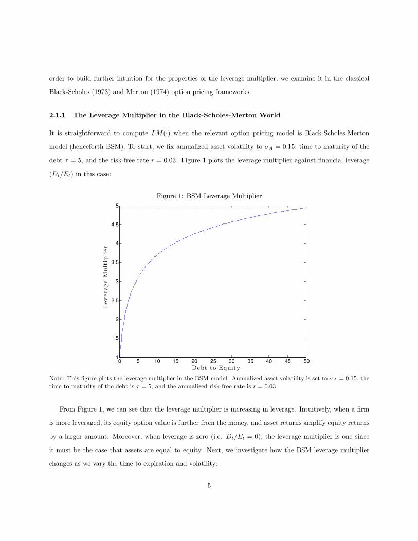
It is straightforward to compute LM(·) when the relevant option pricing model is Black-Scholes-Merton

model (henceforth BSM). To start, we fix annualized asset volatility to �A = 0.15, time to maturity of the

debt ⌧ = 5, and the risk-free rate r = 0.03. Figure 1 plots the leverage multiplier against financial leverage

(Dt/Et) in this case:

Figure 1: BSM Leverage Multiplier

0 5 10 15 20 25 30 35 40 45 501

1.5

2

2.5

3

3.5

4

4.5

5

Debt to Equity

LeverageMultiplier

Note: This figure plots the leverage multiplier in the BSM model. Annualized asset volatility is set to �A = 0.15, thetime to maturity of the debt is ⌧ = 5, and the annualized risk-free rate is r = 0.03

From Figure 1, we can see that the leverage multiplier is increasing in leverage. Intuitively, when a firm

is more leveraged, its equity option value is further from the money, and asset returns amplify equity returns

by a larger amount. Moreover, when leverage is zero (i.e. Dt/Et = 0), the leverage multiplier is one since

it must be the case that assets are equal to equity. Next, we investigate how the BSM leverage multiplier

changes as we vary the time to expiration and volatility:

5

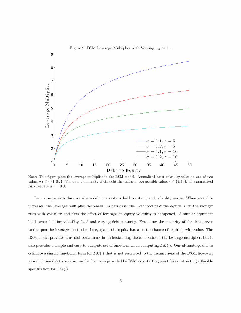
Figure 2: BSM Leverage Multiplier with Varying �A and ⌧

0 5 10 15 20 25 30 35 40 45 501

2

3

4

5

6

7

8

9

Debt to Equity

LeverageMultiplier

! = 0 .1 , " = 5

! = 0 .2 , " = 5

! = 0 .1 , " = 10

! = 0 .2 , " = 10

Note: This figure plots the leverage multiplier in the BSM model. Annualized asset volatility takes on one of twovalues �A 2 {0.1, 0.2}. The time to maturity of the debt also takes on two possible values ⌧ 2 {5, 10}. The annualizedrisk-free rate is r = 0.03

Let us begin with the case where debt maturity is held constant, and volatility varies. When volatility

increases, the leverage multiplier decreases. In this case, the likelihood that the equity is “in the money”

rises with volatility and thus the effect of leverage on equity volatility is dampened. A similar argument

holds when holding volatility fixed and varying debt maturity. Extending the maturity of the debt serves

to dampen the leverage multiplier since, again, the equity has a better chance of expiring with value. The

BSM model provides a usesful benchmark in understanding the economics of the leverage multiplier, but it

also provides a simple and easy to compute set of functions when computing LM(·). Our ultimate goal is to

estimate a simple functional form for LM(·) that is not restricted to the assumptions of the BSM; however,

as we will see shortly we can use the functions provided by BSM as a starting point for constructing a flexible

specification for LM(·).

6

2.2 A Flexible Leverage Multiplier

In the derivation of Equation (4), we did not assign specific functions to g(·) and �t. Define gBSM(·) and

�

BSMt as the BSM inverse call and delta functions, respectively. We then propose the following specification

for the leverage multiplier:

LM⇣Dt/Et,�

fA,t, ⌧, rt;�

⌘=

�

BSMt

⇣Et/Dt, 1,�

fA,t, ⌧, rt

⌘⇥ gBS

⇣Et/Dt, 1,�

fA,t, ⌧, rt

⌘⇥ Dt

Et

��(7)

In this case, � is the departure from the BSM model. When taking our model to data, it will be an

estimated parameter. One advantage of our proposed leverage multiplier in (7) is its simplicity in terms

of computation, as the BSM delta and inverse call functions are well-known. Raising the BSM leverage

multiplier to an arbitrary power also preserves a necessary condition for LM(·) to have a value of one when

leverage is zero. It is worth emphasizing that our leverage multiplier simply uses the BSM functions. For

example, in a BSM world, gBS(·) would be interpreted as the asset to debt ratio, whereas for our model it

is simply a function. Similarly, the BSM �

BSMt in our specification is not interpreted as the correct hedge

ratio, but again merely serves as a function for our purposes. Let us now examine how our leverage multiplier

changes for different values of �, which we plot below in Figure 3:

7

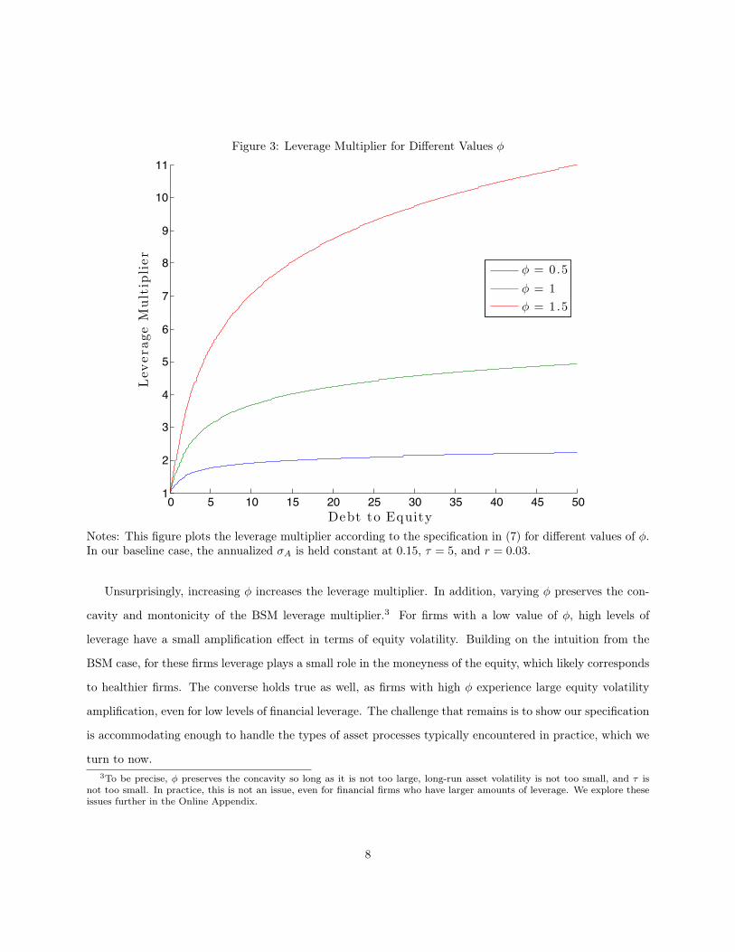
Figure 3: Leverage Multiplier for Different Values �

0 5 10 15 20 25 30 35 40 45 501

2

3

4

5

6

7

8

9

10

11

Debt to Equity

LeverageMultiplier

! = 0 .5

! = 1

! = 1 .5

Notes: This figure plots the leverage multiplier according to the specification in (7) for different values of �.In our baseline case, the annualized �A is held constant at 0.15, ⌧ = 5, and r = 0.03.

Unsurprisingly, increasing � increases the leverage multiplier. In addition, varying � preserves the con-

cavity and montonicity of the BSM leverage multiplier.3 For firms with a low value of �, high levels of

leverage have a small amplification effect in terms of equity volatility. Building on the intuition from the

BSM case, for these firms leverage plays a small role in the moneyness of the equity, which likely corresponds

to healthier firms. The converse holds true as well, as firms with high � experience large equity volatility

amplification, even for low levels of financial leverage. The challenge that remains is to show our specification

is accommodating enough to handle the types of asset processes typically encountered in practice, which we

turn to now.3To be precise, � preserves the concavity so long as it is not too large, long-run asset volatility is not too small, and ⌧ is

not too small. In practice, this is not an issue, even for financial firms who have larger amounts of leverage. We explore theseissues further in the Online Appendix.

8

2.2.1 Is Our Leverage Multiplier Plausible with Stochastic Volatility and/or Non-Normality?

In order to access the plausibility of our leverage multiplier, we conduct a Monte Carlo exercise. First, we

assume a risk-neutral return process for assets. In our simulations, we adopt four different asset processes: 1)

a GARCH process with normally distributed innovations, 2) a GARCH process with t distributed innovations,

3) an asymmetric GARCH process with normally distributed innovations, and 4) an asymmetric GARCH

process with t distributed errors.4 For completeness, we present these recursive volatility models below:

GARCH : �2A,t = ! + ↵r2A,t�1 + ��2

A,t�1

GJR : �2A,t = ! + ↵r2A,t�1 + �r2A,t�11rA,t�1<0 + ��2

A,t�1

The GJR process captures the familiar pattern in equity returns of negative correlation between volatility

and returns, and this correlation is captured by the asymmetry parameter, �. In our parameterization of

these processes, we set the asymmetry parameter to be quite large, as this is one way to capture how risk-

aversion affects the risk-neutral asset process. In addition, for the models with t distributed innovations, we

set the degrees of freedom to six in order to fatten the tails of the asset return process. In order to ensure

comparability across models within our simulation, we change ! so that the unconditional volatility of all

the processes is 15% annually. Table 1 summarizes our parametrization:

ParameterModel ↵ � �

GARCH with Normal Errors 0.07 - 0.92GARCH with t Errors 0.07 - 0.92

GJR with Normal Errors 0.022 0.18 0.884GJR with t Errors 0.022 0.18 0.884

Table 1: Parameterizations for Simulated Asset Processes

For each process, we simulate the asset process 10,000 times from an initial asset value of A0 = 1. We

assume the debt matures in two years and for simplicity set the risk-free rate to zero. The simulation

generates a set of terminal values AT , which generates an equity value for each value of debt D.5 We then

compute numerical derivatives to compute how the equity value changes with respect to A0. Finally, we

compute the leverage multiplier implied by each asset return process, and plot it against the implied financial4The asymmetric GARCH process we use is the so-called GJR process of Golston et al. (1992).5i.e. E =

110,000

P10,000i=1 max(AT,i �D, 0), where i is the index for each simulation run.

9

leverage in Figure 4:

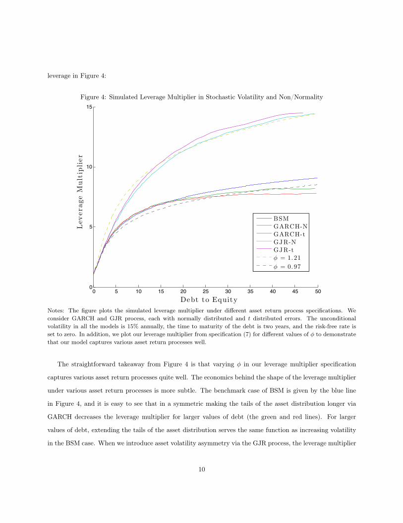
Figure 4: Simulated Leverage Multiplier in Stochastic Volatility and Non/Normality

0 5 10 15 20 25 30 35 40 45 500

5

10

15

Debt to Equity

LeverageMultiplier

BSM

GARCH-N

GARCH-t

GJR-N

GJR-t

! = 1.21

! = 0.97

Notes: The figure plots the simulated leverage multiplier under different asset return process specifications. Weconsider GARCH and GJR process, each with normally distributed and t distributed errors. The unconditionalvolatility in all the models is 15% annually, the time to maturity of the debt is two years, and the risk-free rate isset to zero. In addition, we plot our leverage multiplier from specification (7) for different values of � to demonstratethat our model captures various asset return processes well.

The straightforward takeaway from Figure 4 is that varying � in our leverage multiplier specification

captures various asset return processes quite well. The economics behind the shape of the leverage multiplier

under various asset return processes is more subtle. The benchmark case of BSM is given by the blue line

in Figure 4, and it is easy to see that in a symmetric making the tails of the asset distribution longer via

GARCH decreases the leverage multiplier for larger values of debt (the green and red lines). For larger

values of debt, extending the tails of the asset distribution serves the same function as increasing volatility

in the BSM case. When we introduce asset volatility asymmetry via the GJR process, the leverage multiplier

10

increases dramatically, relative to the BSM benchmark (turquoise and purple lines). Volatility asymmetry

effectively makes the figure asset distribution left skewed, which shortens the right tail of the distribution

and increases the leverage multiplier. In this case, leverage has a larger amplification on equity volatility

because high leverage corresponds to a much smaller likelihood the equity expires “in the money”. As is

clear from the yellow dotted line, increasing � in our model for the leverage multiplier matches this pattern

well. Overall, the simulation exercise summarized by Figure 4 demonstrates that our specification is flexible

enough to capture departures from constant volatility and conditionally normally distributed returns.6

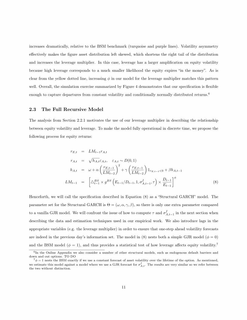
2.3 The Full Recursive Model

The analysis from Section 2.2.1 motivates the use of our leverage multiplier in describing the relationship

between equity volatility and leverage. To make the model fully operational in discrete time, we propose the

following process for equity returns:

rE,t = LMt�1rA,t

rA,t =

phA,t"A,t, "A,t ⇠ D(0, 1)

hA,t = ! + ↵

✓rE,t�1

LMt�2

◆2

+ �

✓rE,t�1

LMt�2

◆1rE,t�1<0 + �hA,t�1

LMt�1 =

4BS

t�1 ⇥ gBS⇣Et�1/Dt�1, 1,�

fA,t�1, ⌧

⌘⇥ Dt�1

Et�1

��(8)

Henceforth, we will call the specification described in Equation (8) as a “Structural GARCH” model. The

parameter set for the Structural GARCH is ⇥ = (!,↵, �,�), so there is only one extra parameter compared

to a vanilla GJR model. We will confront the issue of how to compute ⌧ and �fA,t�1 in the next section when

describing the data and estimation techniques used in our empirical work. We also introduce lags in the

appropriate variables (e.g. the leverage multiplier) in order to ensure that one-step ahead volatility forecasts

are indeed in the previous day’s information set. The model in (8) nests both a simple GJR model (� = 0)

and the BSM model (� = 1), and thus provides a statistical test of how leverage affects equity volatility.7

6In the Online Appendix we also consider a number of other structural models, such as endogenous default barriers anddown and out options. TO DO

7� = 1 nests the BSM exactly if we use a constant forecast of asset volatility over the lifetime of the option. As mentioned,we estimate this model against a model where we use a GJR forecast for �f

A,t. The results are very similar so we refer betweenthe two without distinction.

11

Importantly, the equity return series will inherit volatility asymmetry from the asset return series, which is

an important feature of equity returns in the data.8 The recursion for equity returns (and asset returns) in

(8) is simple and straightforward to compute, yet powerful. For example, when simulating this model, if a

series of negative asset returns is realized (and hence negative asset returns since they share the same shock)

volatility rises due to the asymmetric specification inherent in the GJR. In that case, leverage also rises,

which increases the leverage multiplier and thus results in an even stronger amplification effect for equity

volatility. As we saw in the recent financial crisis, this was a key feature of the data, particularly for highly

leverage financial firms. Additionally, by letting � vary from firm to firm, we effectively allow a different

option pricing model to apply to the capital structure of each firm. This flexibility is difficult to achieve if

one imposes an option pricing model on the data a priori since, as we showed, � allows us to move across

different classes of option pricing models. Furthermore, to the extent that our leverage multiplier form

captures various option pricing models, then the Structural GARCH allows us to infer a high frequency asset

return series with stochastic volatility in a relatively model-free way. Later, this will prove to be extremely

useful for a number of applications of the model.

3 Data Description and Estimation Details

We now turn to estimating the Structural Model using equity return data. In order to compute the leverage

multiplier, we also need balance sheet information, which we obtain from Bloomberg. In particular, define

Dt as the book value of debt at time t. In order to avoid estimation issues that are inherent with quarterly

data, we smooth the book value of debt using an exponential average with smoothing parameter of 0.01.

This smoothing parameter value implies a half-life of approximately seventy days in terms of the weights of

the exponential average, which seems reasonable for quarterly data. When estimating the full model, we use

quasi-maximum likelihood and the associated standard errors for parameter estimates. In order to ensure

a global optimum is reached, we also conduct each maximum likelihood optimization over a grid of twenty

four different starting values.9

The set of firms we analyze are financial firms.10 The reason we focus on financial firms is twofold. First,8For example, it is has been shown that a GJR process for equity can replicate features of equity option data like the

volatility smirk.9The Matlab code for estimation of the model via QMLE with the correct standard errors is available upon request.

10A full description of the set of firms is contained in the Appendix.

12

these firms typically have extraordinarily high leverage and structural models have failed to model these

firms well, which makes them an attractive sector to study. Second, given the high volatility in the recent

crisis that was accompanied by unprecedented leverage, this set of firms presents an important sector to

model from a systemic risk and policy perspective. To this end, one of the applications of our model that

we will explore in later sections involve systemic risk measurement of financials. In future work, we hope to

extend the set of firms we analyze. The remaining issues are how to treat the time to maturity of the debt

⌧ and the asset volatility over the life of the debt �fA,t.

Time to Maturity of the Debt The leverage multiplier requires as an input a time to maturity of the

debt. As the book value of debt combines a number of different debt maturities, we simply iterate over

different ⌧ during estimation. Specifically, we estimate the model for ⌧ 2 [1, 30], restricting ⌧ to take on

integer values. We keep the version of the model that attains the highest log-likelihood function.11

Asset Volatility over Life of Debt We take two different approaches for the computing the value of

�fA,t. The first is to use the unconditional volatility implied by the asset volatility series corresponding to

the unconditional volatility of a GJR process. Using a constant �fA,t in fact completely eliminates any issues

in ignoring the “vega” terms in our motivating derivation of the leverage multiplier (see Equation (2)). The

second approach is to use the GJR forecast over the life of the debt at each date t. It is straightforward to

derive the closed form expression for this forecast. In estimating the full model, we use both approaches for

�fA,t and choose the model with the highest likelihood. That is, we estimate the model over all ranges of ⌧

for each type of �fA,t and choose the model with the highest likelihood.

4 Empirical Results

4.1 Cross-Sectional Summary

We being by presenting a cross-sectional summary of the estimation results. Since the main contribution of

this paper is the leverage multiplier, Figure 5 plots the estimated time-series of the lower quartile, median,

and upper quartile leverage multipliers, across all firms.11TO DO: Confidence intervals for ⌧ using concentrated likelihood function.

13

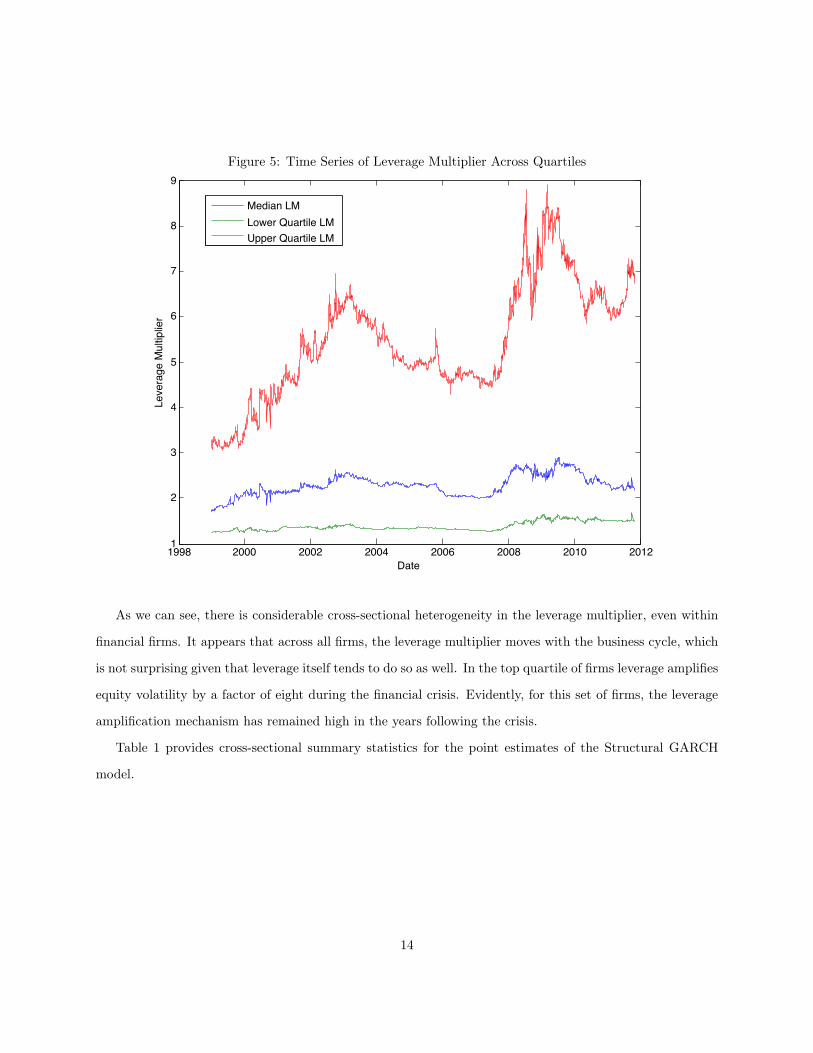
Figure 5: Time Series of Leverage Multiplier Across Quartiles

1998 2000 2002 2004 2006 2008 2010 20121

2

3

4

5

6

7

8

9

Date

Leve

rage

Mul

tiplie

r

Median LMLower Quartile LMUpper Quartile LM

As we can see, there is considerable cross-sectional heterogeneity in the leverage multiplier, even within

financial firms. It appears that across all firms, the leverage multiplier moves with the business cycle, which

is not surprising given that leverage itself tends to do so as well. In the top quartile of firms leverage amplifies

equity volatility by a factor of eight during the financial crisis. Evidently, for this set of firms, the leverage

amplification mechanism has remained high in the years following the crisis.

Table 1 provides cross-sectional summary statistics for the point estimates of the Structural GARCH

model.

14

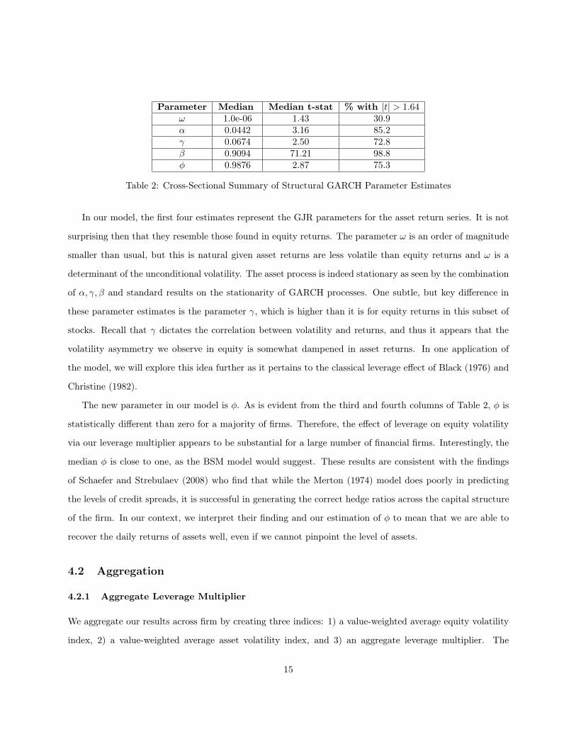
Parameter Median Median t-stat % with |t| > 1.64! 1.0e-06 1.43 30.9↵ 0.0442 3.16 85.2� 0.0674 2.50 72.8� 0.9094 71.21 98.8� 0.9876 2.87 75.3

Table 2: Cross-Sectional Summary of Structural GARCH Parameter Estimates

In our model, the first four estimates represent the GJR parameters for the asset return series. It is not

surprising then that they resemble those found in equity returns. The parameter ! is an order of magnitude

smaller than usual, but this is natural given asset returns are less volatile than equity returns and ! is a

determinant of the unconditional volatility. The asset process is indeed stationary as seen by the combination

of ↵, �,� and standard results on the stationarity of GARCH processes. One subtle, but key difference in

these parameter estimates is the parameter �, which is higher than it is for equity returns in this subset of

stocks. Recall that � dictates the correlation between volatility and returns, and thus it appears that the

volatility asymmetry we observe in equity is somewhat dampened in asset returns. In one application of

the model, we will explore this idea further as it pertains to the classical leverage effect of Black (1976) and

Christine (1982).

The new parameter in our model is �. As is evident from the third and fourth columns of Table 2, � is

statistically different than zero for a majority of firms. Therefore, the effect of leverage on equity volatility

via our leverage multiplier appears to be substantial for a large number of financial firms. Interestingly, the

median � is close to one, as the BSM model would suggest. These results are consistent with the findings

of Schaefer and Strebulaev (2008) who find that while the Merton (1974) model does poorly in predicting

the levels of credit spreads, it is successful in generating the correct hedge ratios across the capital structure

of the firm. In our context, we interpret their finding and our estimation of � to mean that we are able to

recover the daily returns of assets well, even if we cannot pinpoint the level of assets.

4.2 Aggregation

4.2.1 Aggregate Leverage Multiplier

We aggregate our results across firm by creating three indices: 1) a value-weighted average equity volatility

index, 2) a value-weighted average asset volatility index, and 3) an aggregate leverage multiplier. The

15

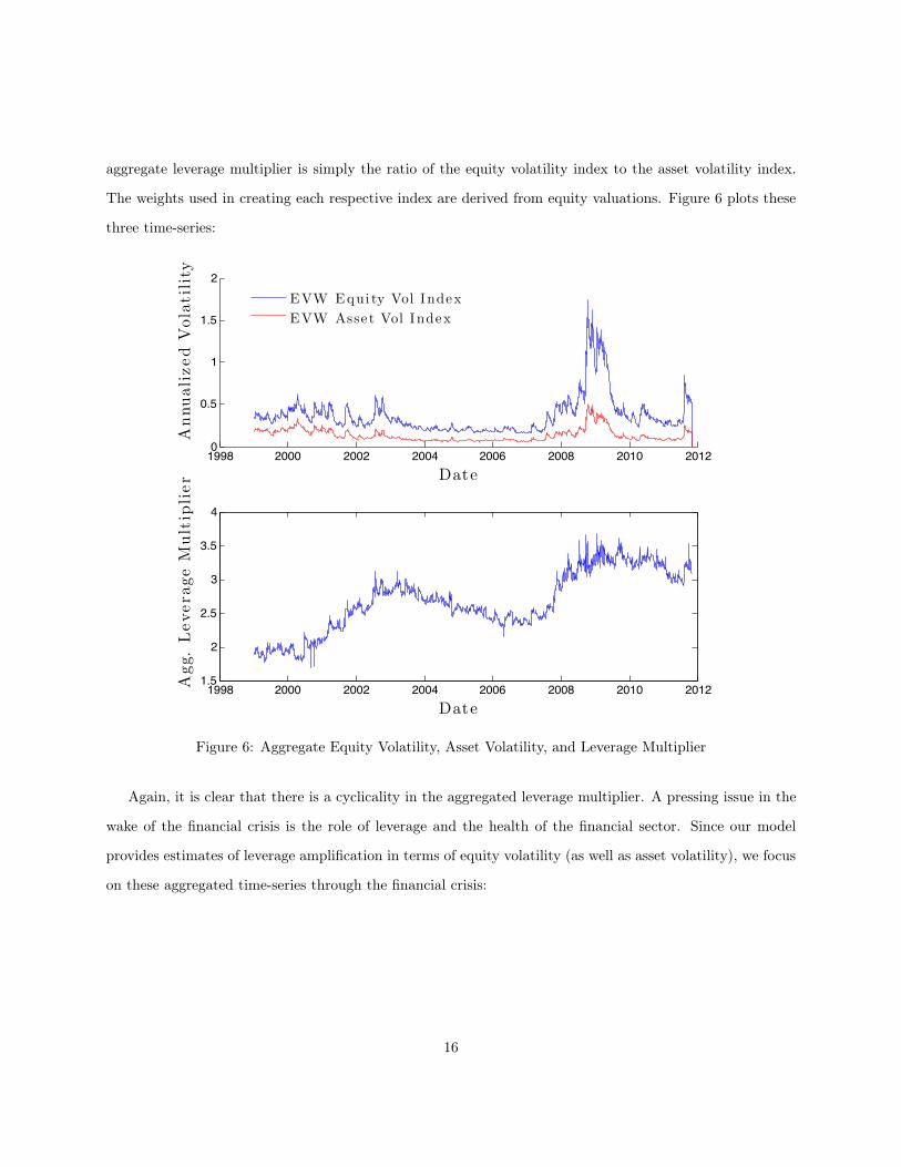
aggregate leverage multiplier is simply the ratio of the equity volatility index to the asset volatility index.

The weights used in creating each respective index are derived from equity valuations. Figure 6 plots these

three time-series:

1998 2000 2002 2004 2006 2008 2010 20120

0.5

1

1.5

2

Date

AnnualizedVolatility

EVW Equi ty Vol Index

EVW Asse t Vol Index

1998 2000 2002 2004 2006 2008 2010 20121.5

2

2.5

3

3.5

4

Date

Agg.LeverageMultiplier

Figure 6: Aggregate Equity Volatility, Asset Volatility, and Leverage Multiplier

Again, it is clear that there is a cyclicality in the aggregated leverage multiplier. A pressing issue in the

wake of the financial crisis is the role of leverage and the health of the financial sector. Since our model

provides estimates of leverage amplification in terms of equity volatility (as well as asset volatility), we focus

on these aggregated time-series through the financial crisis:

16

2007 2008 2009 20100

0.5

1

1.5

2

Date

AnnualizedVolatility

EW Equi ty Vol Index

EW Asse t Vol Index

2007 2008 2009 20102

2.5

3

3.5

4

Date

Agg.LeverageMultiplier

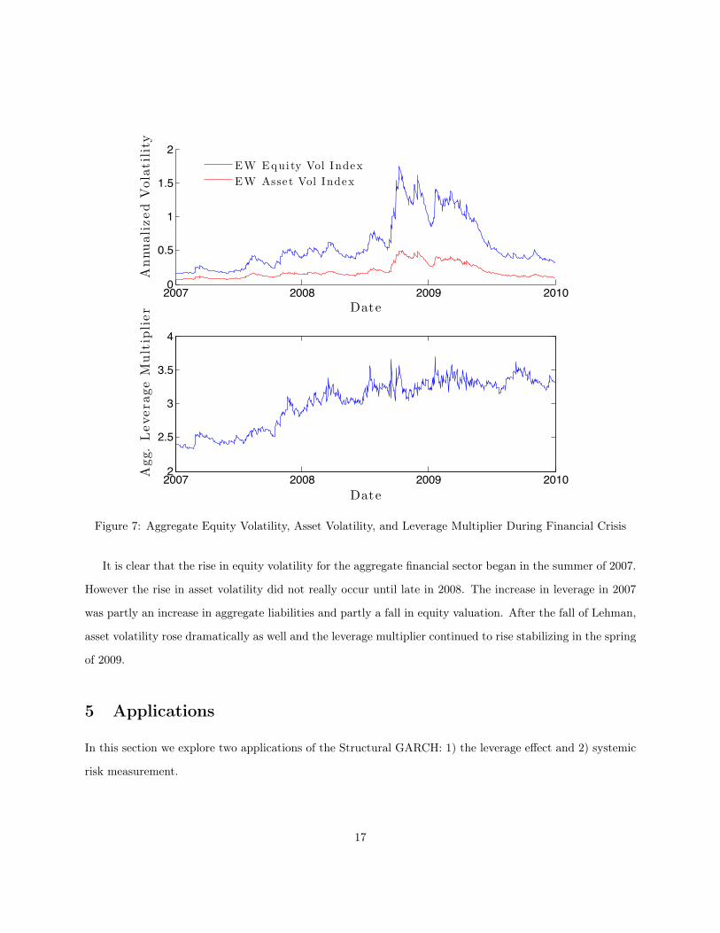
Figure 7: Aggregate Equity Volatility, Asset Volatility, and Leverage Multiplier During Financial Crisis

It is clear that the rise in equity volatility for the aggregate financial sector began in the summer of 2007.

However the rise in asset volatility did not really occur until late in 2008. The increase in leverage in 2007

was partly an increase in aggregate liabilities and partly a fall in equity valuation. After the fall of Lehman,

asset volatility rose dramatically as well and the leverage multiplier continued to rise stabilizing in the spring

of 2009.

5 Applications

In this section we explore two applications of the Structural GARCH: 1) the leverage effect and 2) systemic

risk measurement.

17

5.1 The Leverage Effect

The leverage effect of Black (1976) and Christie (1982) documents the negative correlation that exists

between equity returns and equity volatility. One possible explanation for this stylized fact is that when

a firm experiences a fall in equity, its financial leverage mechanically rises, the company becomes riskier,

and hence volatility rises. A second explanation points to the role of risk premia in describing the negative

correlation between equity returns and equity volatility (e.g. French et al. (1987)). In this explanation, a rise

in future volatility raises the required return on equity, leading to an immediate decline in the stock price.

The Structural GARCH model provides a natural framework to explore these issues econometrically.12

Recall that the Structural GARCH model delivers an estimate of the daily return of assets.13 Since

any correlation between asset volatility and asset returns can not be due to financial leverage, then any

correlation that remains can be attributed to a risk-premium argument. In fact, the � parameter in the

GJR volatility model is one way to capture this correlation (e.g. a higher � corresponds to more negative

correlation). Therefore, we would expect the GJR � estimated from equity returns to be larger than the same

parameter estimated from asset returns. Indeed, the median � for equity returns is 0.0846 and the median �

for asset returns is 0.0674; thus, financial leverage accounts for roughly 23% of the so-called leverage effect,

at least for our subsample of firms.

To put a bit more structure on the implications of Structural GARCH and the leverage effect, we run

the following cross-sectional regression:

�E,i � �A,i = a+ b⇥D/Ei + errori (9)

where �E,i and �A,i are the estimated GJR asymmetry parameter for firm i’s equity returns and firm i’s

asset returns, respectively. D/Ei is the median debt to equity ratio for firm i over the sample period. The

logic behind the regression in (9) is simple: firms with higher leverage should experience a larger reduction

in volatility asymmetry after unlevering the firm. Table 3 presents the results:12Other econometric studies of the leverage effect include Bekaert and Wu (2001). A key divergence in our approach is that

we allow debt for the firm to be risky, as in the Merton (1974) model.13Again, this relies on a few assumptions. First, our specification ignores the effect of changes in long-run asset volatility

on daily equity returns. Second, we assume that the book value of debt adequately captures the outstanding liabilities of thefirm. For example, we do not consider non-debt liabilities in our baseline specification. Still, the Structural GARCH model is,at worst, effective in at least partially unlevering the firm.

18

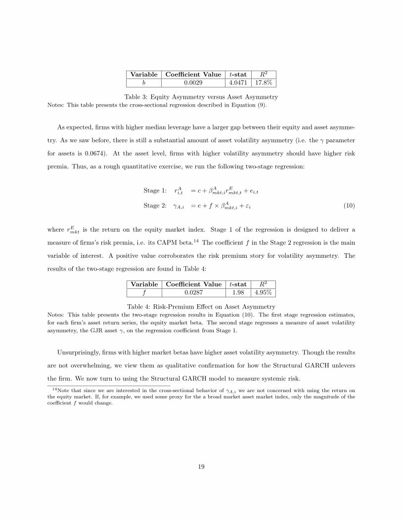
Variable Coefficient Value t-stat R2

b 0.0029 4.0471 17.8%

Table 3: Equity Asymmetry versus Asset AsymmetryNotes: This table presents the cross-sectional regression described in Equation (9).

As expected, firms with higher median leverage have a larger gap between their equity and asset asymme-

try. As we saw before, there is still a substantial amount of asset volatility asymmetry (i.e. the � parameter

for assets is 0.0674). At the asset level, firms with higher volatility asymmetry should have higher risk

premia. Thus, as a rough quantitative exercise, we run the following two-stage regression:

Stage 1: rAi,t = c+ �Amkt,ir

Emkt,t + ei,t

Stage 2: �A,i = e+ f ⇥ �Amkt,i + "i (10)

where rEmkt is the return on the equity market index. Stage 1 of the regression is designed to deliver a

measure of firms’s risk premia, i.e. its CAPM beta.14 The coefficient f in the Stage 2 regression is the main

variable of interest. A positive value corroborates the risk premium story for volatility asymmetry. The

results of the two-stage regression are found in Table 4:

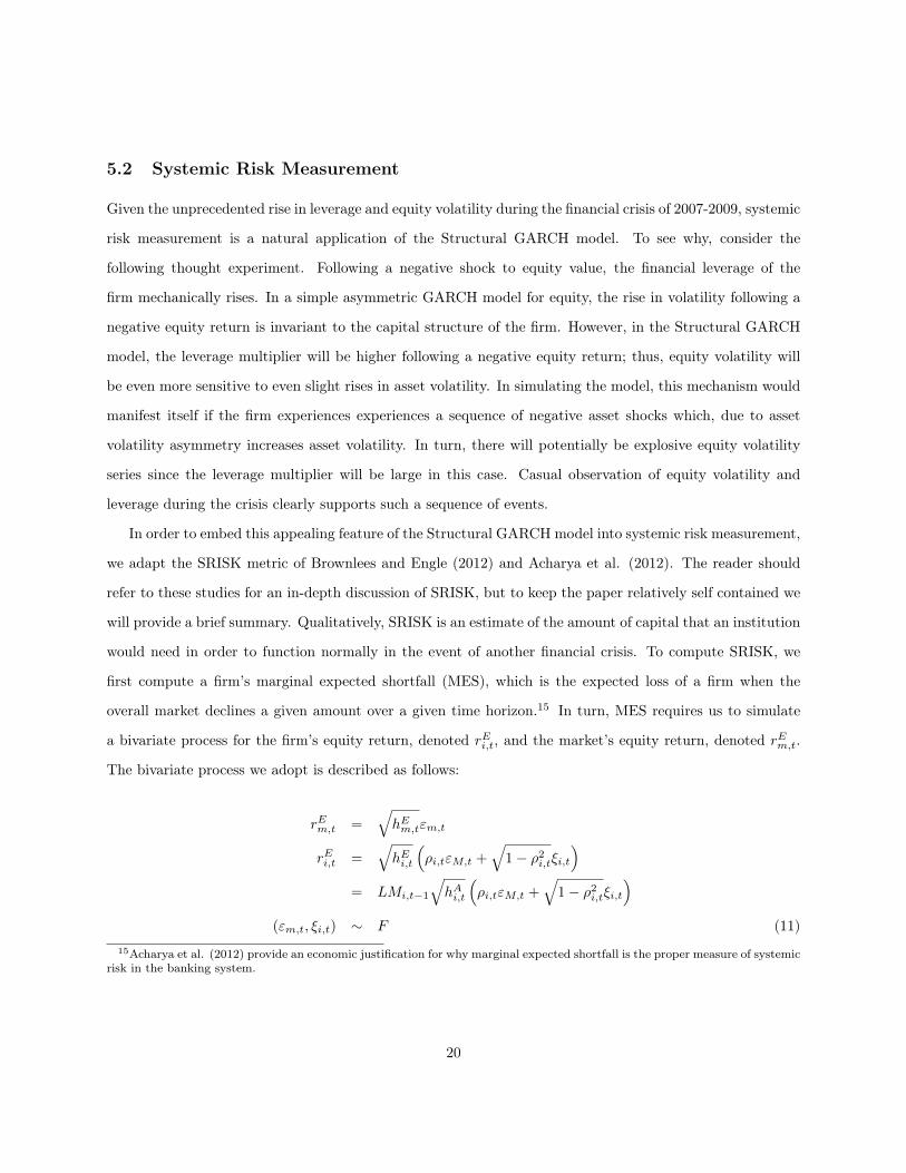
Variable Coefficient Value t-stat R2

f 0.0287 1.98 4.95%

Table 4: Risk-Premium Effect on Asset AsymmetryNotes: This table presents the two-stage regression results in Equation (10). The first stage regression estimates,for each firm’s asset return series, the equity market beta. The second stage regresses a measure of asset volatilityasymmetry, the GJR asset �, on the regression coefficient from Stage 1.

Unsurprisingly, firms with higher market betas have higher asset volatility asymmetry. Though the results

are not overwhelming, we view them as qualitative confirmation for how the Structural GARCH unlevers

the firm. We now turn to using the Structural GARCH model to measure systemic risk.14Note that since we are interested in the cross-sectional behavior of �A,i we are not concerned with using the return on

the equity market. If, for example, we used some proxy for the a broad market asset market index, only the magnitude of thecoefficient f would change.

19

5.2 Systemic Risk Measurement

Given the unprecedented rise in leverage and equity volatility during the financial crisis of 2007-2009, systemic

risk measurement is a natural application of the Structural GARCH model. To see why, consider the

following thought experiment. Following a negative shock to equity value, the financial leverage of the

firm mechanically rises. In a simple asymmetric GARCH model for equity, the rise in volatility following a

negative equity return is invariant to the capital structure of the firm. However, in the Structural GARCH

model, the leverage multiplier will be higher following a negative equity return; thus, equity volatility will

be even more sensitive to even slight rises in asset volatility. In simulating the model, this mechanism would

manifest itself if the firm experiences experiences a sequence of negative asset shocks which, due to asset

volatility asymmetry increases asset volatility. In turn, there will potentially be explosive equity volatility

series since the leverage multiplier will be large in this case. Casual observation of equity volatility and

leverage during the crisis clearly supports such a sequence of events.

In order to embed this appealing feature of the Structural GARCH model into systemic risk measurement,

we adapt the SRISK metric of Brownlees and Engle (2012) and Acharya et al. (2012). The reader should

refer to these studies for an in-depth discussion of SRISK, but to keep the paper relatively self contained we

will provide a brief summary. Qualitatively, SRISK is an estimate of the amount of capital that an institution

would need in order to function normally in the event of another financial crisis. To compute SRISK, we

first compute a firm’s marginal expected shortfall (MES), which is the expected loss of a firm when the

overall market declines a given amount over a given time horizon.15 In turn, MES requires us to simulate

a bivariate process for the firm’s equity return, denoted rEi,t, and the market’s equity return, denoted rEm,t.

The bivariate process we adopt is described as follows:

rEm,t =

qhEm,t"m,t

rEi,t =

qhEi,t

⇣⇢i,t"M,t +

q1� ⇢2i,t⇠i,t

⌘

= LMi,t�1

qhAi,t

⇣⇢i,t"M,t +

q1� ⇢2i,t⇠i,t

⌘

("m,t, ⇠i,t) ⇠ F (11)15Acharya et al. (2012) provide an economic justification for why marginal expected shortfall is the proper measure of systemic

risk in the banking system.

20

where the shocks ("m,t, ⇠i,t) are independent and identically distributed over time and have zero mean, unit

variance, and zero covariance. We do not assume the two shocks are independent, however, and allow them to

have extreme tail dependence nonparametrically.16 The processes hEm,t, h

Ei,t and ⇢i,t represent the conditional

variance of the market, the conditional variance of the firm, and the conditional correlation between the

market and the firm, respectively. It is also worth emphasizing that, due to the Structural GARCH model,

we are really estimating correlations between shocks to the equity market index and shocks to firm asset

returns. Generically, once the bivariate process in (11) is fully specified, we compute a 6-month MES

(henceforth LRMES for “long-run” marginal expected shortfall) by simulating the joint processes for the firm

and the market (with bootstrapped shocks) and conditioning on the event that the market declines by 40%.

Incorporating the Structural GARCH model into LRMES is therefore very simple. As stated in Equation

(11), we simply assume the volatility process for firm equity returns follows a Structural GARCH model.

Finally, we assume that equity market volatility follows a familiar GJR(1,1) process and that correlations

follow a DCC(1,1) model.

Once we have an estimate for the LRMES of a firm on a given day, we compute its capital shortfall in a

crisis as follows:

CSi,t = kDebti,t � (1� k)(1� LRMESi,t)Ei,t (12)

where Debti,t is the book value of debt outstanding on the firm, Ei,t is the market value of equity, and k is

a prudential level of equity relative to assets. In our applications, we take k = 8% and, as is conventional in

risk metrics such as VaR, we use positive values of LRMESi,t to represent declines in the firm’s value. For

example, if firm i is expected to lose 60% of its equity in a crisis, its LRMES will be 60%. Thus, positive

values of capital shortfall mean that the firm will be short of capital in a crisis. Finally, we define the SRISK

of a firm as:

SRISKi,t = max(CSi,t, 0)

The parameters governing the market volatility and firm-market correlation are estimated recursively and

allowed to change daily. However, due to the computational burden of estimating the Structural GARCH

recursively each day, we use the full sample to estimate the Structural GARCH parameters. In future versions

of SRISK measurement with Structural GARCH, we hope to estimate all parameters of the bivariate process16See Brownlees and Engle (2012) for complete details.

21

recursively. The calculation of SRISK for the firms analyzed in Section 3 can be found at the following web

address: INSERT LINK.

6 Extensions and Conclusion

6.1 Granular Debt Measurement

One obvious way to extend the Structural GARCH model is to allow for different types of debt to determine

the strike in the Merton (1974) model. That is, instead of using the book value of debt in the option pricing

formulas, we can further decompose debt. For example, balance sheet information readily delivers short term

liabilities, long term liabilities, and non-debt liabilities. Thus, we could add extra parameters to the model

as pseudo-weights on each debt component:

Dt = ✓1 ⇥ LT Debtt + ✓2 ⇥ ST Debtt + ✓3 ⇥ Non-Debt Liabilitiest (13)

In this case, ✓1, ✓2, ✓3 are estimated parameters (with an appropriate normalization). Duan (1996) in fact

finds this type of decomposition to be extremely useful in fitting the data in the context of maximum

likelihood estimation of the static Merton (1974) model. Decomposing the debt has obvious advantages for

the subset of firms we examine, i.e. financial firms, given that many broker-dealers like Bear Stearns and

Lehman Brothers relied heavily on short term debt. For firms with large deposit bases, like commercial

banks, the debt decomposition would also help fit the data in this regard.

6.2 Additional Parameters for the Leverage Multiplier

It is easy to see from the derivation Equation (4) that the leverage multiplier in a generic setting is simply

the delta of the option multiplied by the inverse call option pricing formula (scaled by leverage). Thus, one

way to view our specification of the leverage multiplier is that power functions of the BSM delta and BSM

inverse call option pricing function are suitable in stochastic volatility and non-normal environments. To see

why, recall that our leverage multiplier specification is, in a reduced form, as follows:

LM(D/E) =

��

BS�� ⇥

✓gBS

(D/E) · DE

◆�

(14)

22

where again �

BS and gBS are the BSM delta and inverse call pricing functions. We choose our parameter �

to match the entire leverage multiplier for an arbitrary asset return generating process, but does this same

parameter of � match the individual hedge ratios and inverse call pricing functions?

To explore this idea further, we again turn to a Monte Carlo exercise. As in Section 2.2.1, we simulate

a variety of stochastic volatility processes for assets and compute the leverage multiplier for different levels

of debt (leverage). Then we choose a reasonable parameter for � from the specification in Equation (7) to

match each of these cases to a reasonable degree. After we settle on a �, we check whether the implied hedge

ratio (e.g.��

BS��) and implied inverse call option pricing function match their simulated counterparts as

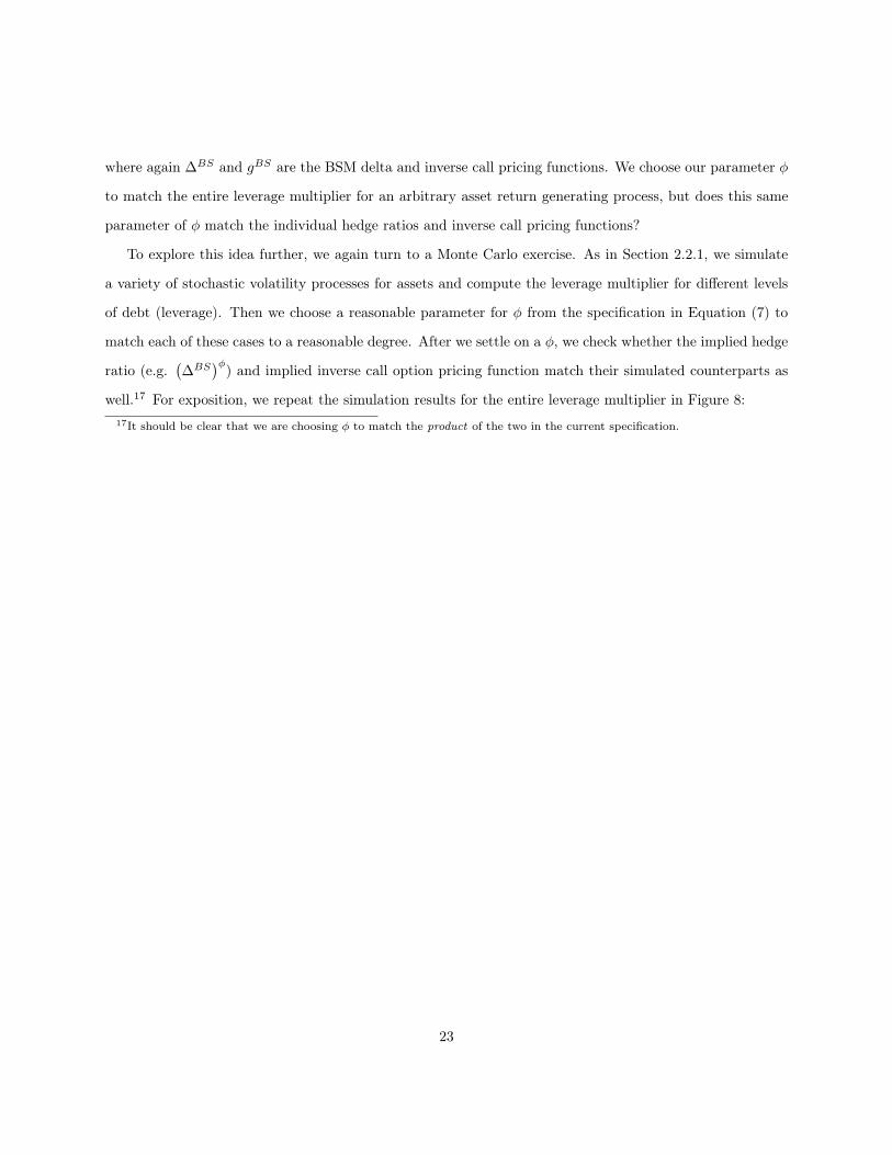
well.17 For exposition, we repeat the simulation results for the entire leverage multiplier in Figure 8:17It should be clear that we are choosing � to match the product of the two in the current specification.

23

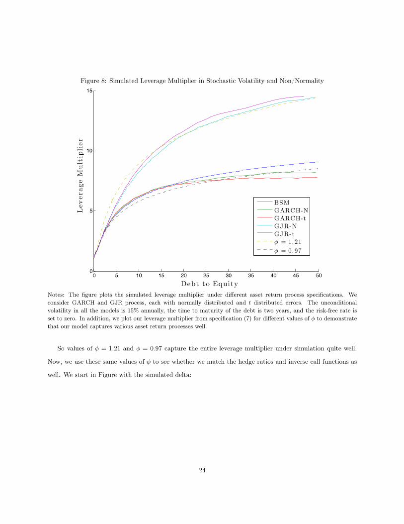
Figure 8: Simulated Leverage Multiplier in Stochastic Volatility and Non/Normality

0 5 10 15 20 25 30 35 40 45 500

5

10

15

Debt to Equity

LeverageMultiplier

BSM

GARCH-N

GARCH-t

GJR-N

GJR-t

! = 1.21

! = 0.97

Notes: The figure plots the simulated leverage multiplier under different asset return process specifications. Weconsider GARCH and GJR process, each with normally distributed and t distributed errors. The unconditionalvolatility in all the models is 15% annually, the time to maturity of the debt is two years, and the risk-free rate isset to zero. In addition, we plot our leverage multiplier from specification (7) for different values of � to demonstratethat our model captures various asset return processes well.

So values of � = 1.21 and � = 0.97 capture the entire leverage multiplier under simulation quite well.

Now, we use these same values of � to see whether we match the hedge ratios and inverse call functions as

well. We start in Figure with the simulated delta:

24

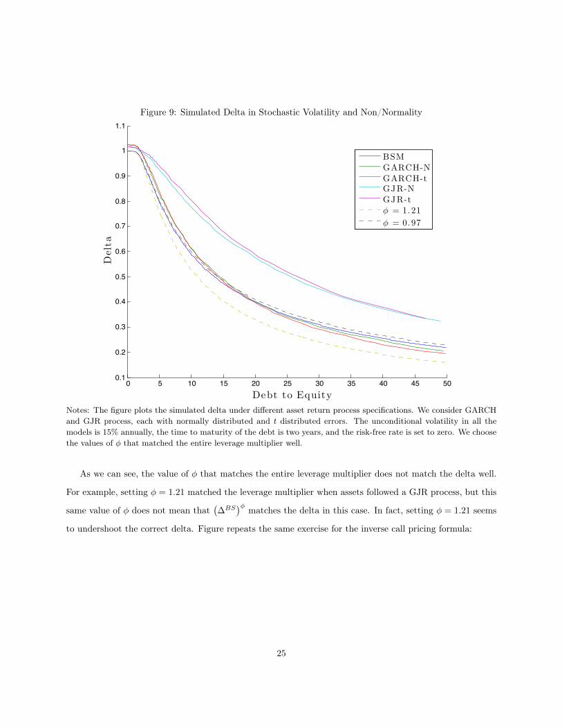
Figure 9: Simulated Delta in Stochastic Volatility and Non/Normality

0 5 10 15 20 25 30 35 40 45 500.1

0.2

0.3

0.4

0.5

0.6

0.7

0.8

0.9

1

1.1

Debt to Equity

Delta

BSM

GARCH-N

GARCH-tGJR-N

GJR-t

! = 1.21

! = 0.97

Notes: The figure plots the simulated delta under different asset return process specifications. We consider GARCHand GJR process, each with normally distributed and t distributed errors. The unconditional volatility in all themodels is 15% annually, the time to maturity of the debt is two years, and the risk-free rate is set to zero. We choosethe values of � that matched the entire leverage multiplier well.

As we can see, the value of � that matches the entire leverage multiplier does not match the delta well.

For example, setting � = 1.21 matched the leverage multiplier when assets followed a GJR process, but this

same value of � does not mean that��

BS�� matches the delta in this case. In fact, setting � = 1.21 seems

to undershoot the correct delta. Figure repeats the same exercise for the inverse call pricing formula:

25

Figure 10: Simulated Delta in Stochastic Volatility and Non/Normality

0 5 10 15 20 25 30 35 40 45 500

10

20

30

40

50

60

Debt to Equity

AssetstoEquity

BSM

GARCH-N

GARCH-tGJR-N

GJR-t

! = 1.21

! = 0.97

Notes: The figure plots the inverse call function under different asset return process specifications. We considerGARCH and GJR process, each with normally distributed and t distributed errors. The unconditional volatility inall the models is 15% annually, the time to maturity of the debt is two years, and the risk-free rate is set to zero. Wechoose the values of � that matched the entire leverage multiplier well.

Unsurprisingly, the values of � that matched the leverage multiplier again do not match the inverse call

option pricing formula. Continuing with the previous example of the GJR process for assets, � = 1.16

overshoots the inverse call function. This makes sense given it undershot the delta, but matched the entire

leverage multiplier, which is the product of the delta and the inverse call function. In light of these results,

a natural extension of our leverage multiplier specification is as follows:

LM⇣Dt/Et,�

fA,t, ⌧, rt;�

⌘=

h�

BSMt

⇣Et/Dt, 1,�

fA,t, ⌧, rt

⌘i�⇥

gBS

⇣Et/Dt, 1,�

fA,t, ⌧, rt

⌘⇥ Dt

Et

��(15)

where now � and � are now estimated parameters. Notice we raise the leverage ratio to the power � because in

26

reality, the leverage multiplier is the delta of the option multiplier by the asset to equity ratio. gBS(·)⇥D/E

is precisely the asset to equity ratio in the BSM model. The model in (15) also has the advantage of nesting

the original Structural GARCH, by restricting � = �.

6.3 Conclusion

This paper has provided a econometric approach to disentangle the effects of leverage on equity volatility.

The Structural GARCH model we propose is rooted in the classical Merton (1974) structural model of credit,

but departs from it in a flexible and parsimonious way. In doing so, we are able to deliver high frequency

asset return and asset volatility series. We applied the model in two different settings (asymmetric volatility

and systemic risk measurement), but there are a variety of applications of the model in both corporate

finance and asset pricing.

27

References

[1] Bekaert, G., and Wu, G. Asymmetric volatility and risk in equity markets. Review of Financial

Studies 13, 1 (2000), 1–42.

[2] Black, F. Studies of stock price volatility changes. Proceedings of the 1976 Meetings of the American

Statistical Association, Business and Economics Statistics Section (1976), 177–181.

[3] Christie, A. A. The stochastic behavior of common stock variances: Value, leverage and interest rate

effects. Journal of financial Economics 10, 4 (1982), 407–432.

[4] Merton, R. C. On the pricing of corporate debt: The risk structure of interest rates*. The Journal of

Finance 29, 2 (1974), 449–470.

[5] Schaefer, S. M., and Strebulaev, I. A. Structural models of credit risk are useful: Evidence from

hedge ratios on corporate bonds. Journal of Financial Economics 90, 1 (2008), 1 – 19.

28

A Appendix: Ignoring Volatility Terms

For exposition, we repeat Equation (2):

dEt

Et= �t ·

At

Dt· Dt

Et· dAt

At+

@f

@�fA,t

· Dt

Et· d�f

A,t (16)

It is straightforward to work out that equity variance will be as follows:

vart

✓dEt

Et

◆=

✓�t

At

Dt· Dt

Et

◆2

vart

✓dAt

At

◆+

✓⌫tDt

Et

◆2

vart

⇣d�f

A,t

⌘

+2

✓�t

At

Dt· Dt

Et

◆✓⌫tDt

Et

◆s

vart

✓dAt

At

◆vart

⇣d�f

A,t

⌘⇥ ⇢t

✓dAt

At, d�f

A,t

◆(17)

where �t = @f⇣At/Dt, 1,�

fA,t, ⌧, r

⌘/@At and ⌫t = @f

⇣At/Dt, 1,�

fA,t, ⌧, r

⌘/@d�f

A,t. In option pricing lingo,

�t is the “delta” of the call option on assets, and ⌫t is the “vega” of the call option on assets.18 In the model

where we set the long run volatility of assets to be the unconditional volatility of the asset GJR process,

this analysis is moot as d�fA,t = 0. Our task now is to show that the last two terms are negligible for the

purposes of modeling equity volatility, when we use the GJR forecast for long run asset volatility.

A.1 Magnitude of Volatility Terms

In the language of the Structural GARCH model we can simply substitute LMt into Equation (17) where it

is appropriate:

vart

✓dEt

Et

◆= (LMt)

2vart

✓dAt

At

◆+

✓⌫tDt

Et

◆2

vart

⇣d�f

A,t

⌘

+2 (LMt)

✓⌫tDt

Et

◆s

vart

✓dAt

At

◆vart

⇣d�f

A,t

⌘⇥ ⇢t

✓dAt

At, d�f

A,t

◆(18)

In order to investigate the magnitude of the terms we ignore (i.e. any term containing ⌫t), we need a

functional form for the sensitivity of the equity value to changes in long run asset volatility. Since we are

only interested in magnitudes, we will use the Black-Scholes vega. It is unlikely that the Black-Scholes vega18To be precise, these are the delta and vega of the option where debt has been normalized to 1.

29

is incorrect by an order of magnitude, so for this exercise it will be sufficient. The next thing we need in

order to quantitatively evaluate Equation (18) are time-series for LMt, dAt/At, and d�fA,t. To be precise, if

we extended the model to include changes in volatility we would undoubtedly obtain different estimates for

these three quantities. Again, since our goal is to assess relative magnitudes, we will simply use the values

delivered by our Structural GARCH model for LMt, dAt/At, and d�fA,t. Formally, we define d�f

A,t as:

d�fA,t =

qhfA,t+1/⌧ �

qhfA,t/⌧

where hfA,t+1 is the forecast of total volatility over the life of the option. Finally, we set the volatility of

volatility to be constant and the correlation between asset returns and volatility to be constant. Under this

assumption, we estimate these quantities using their in-sample moments.

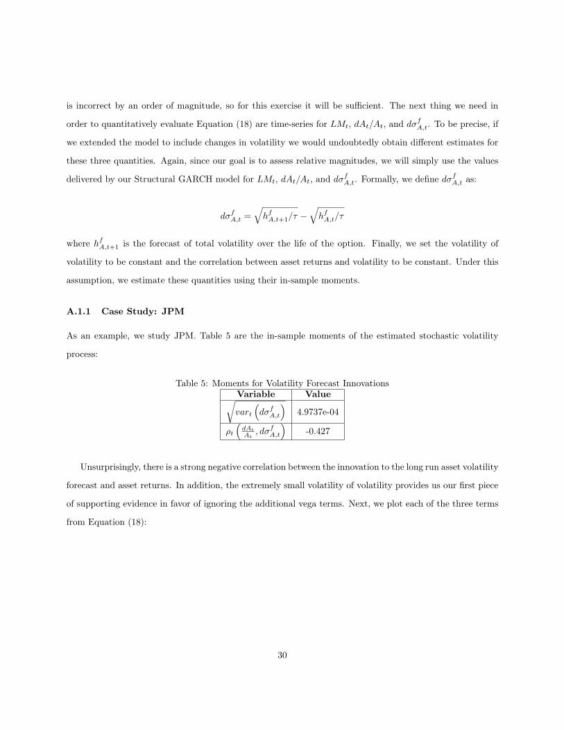
A.1.1 Case Study: JPM

As an example, we study JPM. Table 5 are the in-sample moments of the estimated stochastic volatility

process:

Table 5: Moments for Volatility Forecast InnovationsVariable Valuervart

⇣d�f

A,t

⌘4.9737e-04

⇢t

⇣dAtAt

, d�fA,t

⌘-0.427

Unsurprisingly, there is a strong negative correlation between the innovation to the long run asset volatility

forecast and asset returns. In addition, the extremely small volatility of volatility provides us our first piece

of supporting evidence in favor of ignoring the additional vega terms. Next, we plot each of the three terms

from Equation (18):

30

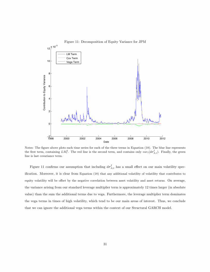
Figure 11: Decomposition of Equity Variance for JPM

1998 2000 2002 2004 2006 2008 2010 2012−2

0

2

4

6

8

10

12 x 10−3

Date

Con

tribu

tion

to E

quity

Var

ianc

e

LM TermCov TermVega Term

Notes: The figure above plots each time series for each of the three terms in Equation (18). The blue line representsthe first term, containing LM2

t . The red line is the second term, and contains only vart(d�fA,t). Finally, the green

line is last covariance term.

Figure 11 confirms our assumption that including d�fA,t has a small effect on our main volatility spec-

ification. Moreover, it is clear from Equation (18) that any additional volatility of volatility that contributes to

equity volatility will be offset by the negative correlation between asset volatility and asset returns. On average,

the variance arising from our standard leverage multiplier term is approximately 12 times larger (in absolute

value) than the sum the additional terms due to vega. Furthermore, the leverage multiplier term dominates

the vega terms in times of high volatility, which tend to be our main areas of interest. Thus, we conclude

that we can ignore the additional vega terms within the context of our Structural GARCH model.

31

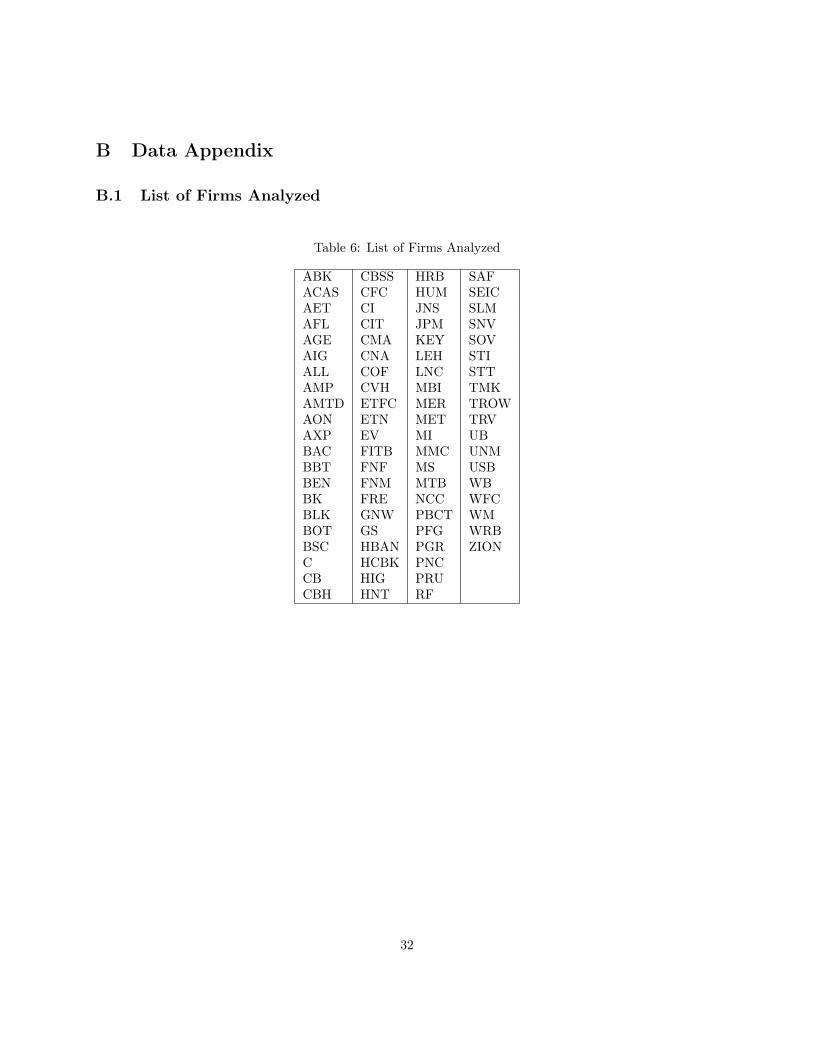
B Data Appendix

B.1 List of Firms Analyzed

Table 6: List of Firms Analyzed

ABK CBSS HRB SAFACAS CFC HUM SEICAET CI JNS SLMAFL CIT JPM SNVAGE CMA KEY SOVAIG CNA LEH STIALL COF LNC STTAMP CVH MBI TMKAMTD ETFC MER TROWAON ETN MET TRVAXP EV MI UBBAC FITB MMC UNMBBT FNF MS USBBEN FNM MTB WBBK FRE NCC WFCBLK GNW PBCT WMBOT GS PFG WRBBSC HBAN PGR ZIONC HCBK PNCCB HIG PRUCBH HNT RF

32