Summative Assignment

Econometrics II

MSc Economics and Finance

April 22, 2015Z0953632

Contents

Contents 2

List of Figures 3

List of Tables 4

1 Testing Nonstationarity 5

2 Volatility Estimation 6

3 VAR Estimation 8

4 Testing Leverage and Volatility Feedback Effects 9

References 22

2

List of Figures

1 The Natural Logarithm of Boeing’s Adjusted Closing Share Prices 11

2 First Differences Plot of the Natural Logarithm of the Share Prices 11

3 SACF of ln(S) . . . . . . . . . . . . . . . . . . . . . . . . . . . . . 12

4 SACF of the First Differences . . . . . . . . . . . . . . . . . . . . 12

5 SPACF of the First Differences . . . . . . . . . . . . . . . . . . . 14

6 Normality Test of GARCH(1,1) Residuals . . . . . . . . . . . . . 16

7 Plot of the Conditional Variance Estimated by GARCH(1,1) . . . 17

8 Correlogram of VAR(5) Residuals . . . . . . . . . . . . . . . . . . 19

9 Impulse Responses . . . . . . . . . . . . . . . . . . . . . . . . . 20

3

List of Tables

1 Coefficients measured by the ADF test . . . . . . . . . . . . . . . 13

2 The ADF Unit Root Test for the Share Prices . . . . . . . . . . . 13

3 The ADF Unit Root Test for the First Differences . . . . . . . . . 13

4 AIC for Different ARMA Orders . . . . . . . . . . . . . . . . . . . 14

5 ARMA(5,3) Model . . . . . . . . . . . . . . . . . . . . . . . . . . 15

6 Testing ARCH Effect . . . . . . . . . . . . . . . . . . . . . . . . . 16

7 Estimated VAR Model (Coefficients marked with asterisks are

Significant at 5%) . . . . . . . . . . . . . . . . . . . . . . . . . . . 18

8 VAR(5) Residual Correlation Matrix . . . . . . . . . . . . . . . . . 18

9 Multivariate Normaility Test of VAR(5) Residuals . . . . . . . . . 20

10 Granger Causality Analysis . . . . . . . . . . . . . . . . . . . . . 21

4

1 Testing Nonstationarity

The adjusted closing share prices of Boeing have been retrieved from Yahoo

Finance for the past five years. The ln plot of the aforementioned time-series is

shown in Figure 1.

The ln(S) process appears to violate the conditions of constant mean and con-

ditional variance of weak stationarity. The first differences plot in figure 2, further

reveals that the process may be first-order integrated. These findings are con-

firmed by the slow decaying SACF plot (fig. 3) of the ln(s) process, which unlike

∆ln(s) (fig. 4) shows the high correlation of the process with its own lags.

Graphical means of testing nonstationarity may be deceiving. A plausible

approach for testing nonstationarity is to start from a general relationship such

as equation (1), which includes an intercept, an autoregressive process of order

p and a time trend, and by conducting appropriate tests (e.g. Perron Sequential

Testing Procedure) simplify to one of the cases of nonstationarity: No drift or no

trend, drift but no trend, both drift and trend.

ln(St) = α + δt+ θln(St−1) +

p−1∑j=1

pj∆ln(St−j) + ut (1)

Dougherty (2011) suggested that the aforementioned general-to-specific ap-

proaches have low power that may lead to ambiguity. A pragmatic approach

for choosing an appropriate Dickey-Fuller test is to analyse the plot of the data

and look for obvious trends.

Evidently, the data has an upward trend. Hence, the appropriate choice of a

Dickey-Fuller test includes a drift and a deterministic trend.

The unit root null hypothesis is

H0 : θ = 1 (2)

against the alternative

HA : |θ| < 1 (3)

5

The number of lags of the ADF test is chosen by Eviews using the Schwarz

Information Criterion to minimize

SIC = log(RSS

T) +

klogT

T= log(

RSS

T) +

(p+ 2)logT

T(4)

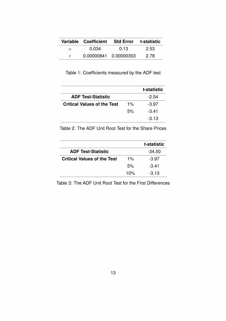
Surprisingly, the ADF test chose 0 lags for the model. Furthermore, as shown

in table 1, the trend and the constant coefficients are highly significant, which

implies the correct choice of the model.

Since the ADF t-statistic in table 2 is not larger in absolute terms than the critical

values of DF with a trend and a constant, the unit root null hypothesis does not

get rejected. Taking the first-differences and conducting the ADF test with no

intercept and no trend yields the t-statistic in table 3, indicating the stationarity

of the data and integration of first order.

2 Volatility Estimation

To estimate the volatility of the share prices, initially an appropriate ARMA model

is chosen. The first differences plot and the unit testing procedure carried out

earlier, indicate that the process is first order integrated and the returns are sta-

tionary. To choose an appropriate ARMA model, the Box-Jenkins approach is

utilised.

The order of the model is determined by choosing the number of parameters

that minimizes the information criterion and yields a parsimonious model. Infor-

mation criterion models are functions of RSS, and penalise adding extra param-

eters. In this case AIC is chosen, which overparameterizes, but produces better

results in practice (Dougherty, 2011).

The SACF and SPACF of the returns (fig. 4 & 5) do not possess any of the

AR and MA ‘signatures’ and are of little help. The information criterion is min-

imised with an ARMA(4,5) model (Table 4). However, the joint-null hypothesis

6

of no autocorrelation gets rejected at 5% level of significance for numerous lags

when diagnosing residuals using Ljung-Box Q-statistic; hence, the next best

model of ARMA(5,3) is chosen, which does not suffer from this issue.

Rt = c+5∑

i=1

φiyt−i +3∑

j=1

θjut−j + ut (5)

Once the ARMA model is determined, the ARCH effect with 5 lags is analysed.

Both the LM-statistic and F-statistics in table 6 are highly significant, suggesting

the existence of ARCH in R and persistence in the variance of returns.

The GARCH(1,1) is estimated

ht = 1.26× 10−5

(4.39)+ 0.097u2t−1

(6.63)

+ 0.846ht−1(38.22)

(6)

All coefficients are highly significant, and the analysis of the correlogram

and Ljung-box Q-statistic at the 36th lag is 36.045 with p-value of 0.14, sug-

gesting that the autocorrelation of squared residuals of the mean (i.e. ARCH

effect) has been captured by the GARCH(1,1) model. The Jarque-Bera test in

figure 6, rejects the null hypothesis of normality of the residuals. Therefore, the

GARCH(1,1) model is estimated again using Robust Standard Errors to obtain

unbiased estimators

ht = 1.10× 10−5

(2.78)+ 0.087u2t−1

(4.29)

+ 0.862ht−1(27.42)

(7)

The graph of the conditional volatility estimated by the model is shown in fig-

ure 7. The sum of the squared residual and variance coefficients in GARCH(1,1)

is 0.95, showing the high persistent (close to 1), yet mean reverting nature of

the volatility model.

7

3 VAR Estimation

For estimating VAR, it is important that the variables are stationary or cointe-

grated. Thus far, our analysis has indicated that both returns and the estimated

volatilities are stationary. Hence, testing cointegration is not necessary, as the

processes do not possess unit roots.

To select the optimal order of the VAR model, such that the errors follow a white

noise process, the objective is to minimise the information criterion, which in

this case is accomplished by choosing a lag of 5 based on MAIC. It is evident

that not all coefficients are statistically significant (table 7). However, before

analysing the estimated model and making conclusions based on t-statistics,

the assumptions of VAR(p) are checked to ensure that the OLS estimation of

the equation is consistent, efficient and approximately normal.

Since the dependent variables are stationary, the no autocorrelation assump-

tion of the error terms is expected to hold. Figure 8 indicates that there is no

substantial autocorrelation. This is consistent with the autocorrelation LM-test

at 5% significance level, which fails to reject the null hypothesis of no autocor-

relation at almost all lags, and the residual correlation matrix in table 8.

Finally, a multivariate normality test with χ2 statistics associated with skewness

and kurtosis in table 9, shows that the error terms are not normally distributed.

Furthermore, the homoscedasticity null hypothesis gets rejected at 5% signifi-

cance with a χ2 statistic of 1171. Nevertheless, according to Sims et al (1990),

the use of t-tests and F-tests is appropriate when the coefficients of interest are

stationary, and given a large sample size, the critical values of a normal distri-

bution may be used.

To interpret the estimated model, impulse responses have been constructed

to analyse the responsiveness of the dependent variables to unit shocks to the

8

error terms. Due to the stationarity of the return and volatility variables, the

estimated VAR is stable and mean-reverting. As expected, figure 9 shows that

the shock effects fade away over time. The highest persistent shock is the

impact of a unit shock to volatility on volatility itself. Furthermore, a unit shock

to the returns leads to an inverse shift in volatility. The impact of a shock to

volatility is small on returns, while a unit shock to the return has a large impact

on returns itself; though the effect fades away exponentially.

4 Testing Leverage and Volatility Feedback Effects

To test whether leverage and volatility feedback effects are present, we wish to

test the null hypotheses

H0 : No volatility feedback effect (8)

H0 : No leverage effect (9)

“The fundamental difference between the leverage and volatility feedback expla-

nations lies in the ‘causality’: the leverage effect explains why a negative return

leads to higher subsequent volatility, whereas the volatility feedback effect justi-

fies how an increase in volatility may result in negative returns”.(Bollerslev et al,

2006)

In earlier section, a VAR(5) model was estimated in which returns and volatilities

are endogenous variables with impacts on one another. The model is

Rt = c+5∑

j=1

αjRt−j +5∑

j=1

βjht−j + ut (10)

ht = c+5∑

j=1

γjht−j +5∑

j=1

δjRt−j + ut (11)

9

To test whether the returns have any significant impact on volatility and vice

versa, the Granger Causality test conducts a joint hypothesis using an F-test

H0 : β1 = β2 = ... = βj = 0 for equation 10 (12)

and

H0 : δ1 = δ2 = ... = δj = 0 for equation 11 (13)

Null-hypothesis (12) does not get rejected (table 10), which implies there is no

volatility feedback effect. The second F-statistic on the other hand is highly

significant, which indicates that returns have a significant impact on volatility.

Furthermore, figure 9 shows that this relationship is inverse, rejecting the no

leverage effect hypothesis.

10

Figure 1: The Natural Logarithm of Boeing’s Adjusted Closing Share Prices

Figure 2: First Differences Plot of the Natural Logarithm of the Share Prices11

Figure 3: SACF of ln(S)

Figure 4: SACF of the First Differences12

Variable Coefficient Std Error t-statistic

α 0.034 0.13 2.53

t 0.00000841 0.00000303 2.78

Table 1: Coefficients measured by the ADF test

t-statistic

ADF Test-Statistic -2.54

Critical Values of the Test 1% -3.97

5% -3.41

-3.13

Table 2: The ADF Unit Root Test for the Share Prices

t-statistic

ADF Test-Statistic -34.50

Critical Values of the Test 1% -3.97

5% -3.41

10% -3.13

Table 3: The ADF Unit Root Test for the First Differences

13

Figure 5: SPACF of the First Differences

ARMA(p,q) q=1 q=2 q=3 q=4 q=5

p=1 -5.5347 -5.5375 -5.5366 -5.5354 -5.5347

p=2 -5.5371 -5.5474 -5.5463 -5.5452 -5.5342

p=3 -5.5356 -5.5359 -5.4782 -5.5465 -5.5322

p=4 -5.5347 -5.5354 -5.5474 -5.5497 -5.5513

p=5 -5.5347 -5.533 -5.5469 -5.5502 -5.5499

Table 4: AIC for Different ARMA Orders

14

Vari

able

cA

R(1

)A

R(2

)A

R(3

)A

R(4

)A

R(5

)M

A(1

)M

A(2

)M

A(3

)

Coe

ffici

ent

0.00

071.

6969

*-1

.594

9*0.

5586

*-0

.002

2-0

.040

2-1

.684

6*1.

5547

*-0

.54*

Std

.Err

or0.

0004

0.22

530.

2655

0.23

430.

0612

0.03

430.

2246

0.25

650.

2057

t-st

atis

tic1.

847.

53-6

.00

2.38

-0.0

3-1

.16

-7.4

96.

06-2

.62

Pro

b(F-

stat

)0.

0001

75

Tabl

e5:

AR

MA

(5,3

)Mod

el

15

Test-Statistic Coefficient p-values

F-Statistic 30.738 0.0000

LM-Test 137.427 0.0000

Table 6: Testing ARCH Effect

Figure 6: Normality Test of GARCH(1,1) Residuals

16

Figu

re7:

Plo

toft

heC

ondi

tiona

lVar

ianc

eE

stim

ated

byG

AR

CH

(1,1

)

17

ht Rt

c 1.32× 10−5∗ 0.000131

(5.86) (0.153)

ht−1 0.984134∗ −11.63049

(34.81) (−1.08)

ht−2 0.064391 34.13301∗

(1.63) (2.27)

ht−3 −0.165896∗ −32.93824∗

(−4.24) (−2.21)

ht−4 0.132047∗ 13.25747

(3.36) (0.89)

ht−5 −0.069701∗ 0.033311

(−2.50) (0.00314)

Rt−1 −0.000452∗ 0.024692

(−6.058) (0.87)

Rt−2 −7.92× 10−5 −0.031109

(−1.05) (−1.082)

Rt−3 −0.000408∗ −0.026362

(−5.39) (−0.918)

Rt−4 −6.21× 10−5 −0.044414

(−0.82) (−1.54)

Rt−5 −0.000187∗ −0.059401∗

(−2.45) (−2.05)

Table 7: Estimated VAR Model (Coefficients marked with asterisks are Signifi-

cant at 5%)

h r

h 1.00 0.00278

r 0.00278 1.00

Table 8: VAR(5) Residual Correlation Matrix

18

Figu

re8:

Cor

relo

gram

ofVA

R(5

)Res

idua

ls

19

Component Skewness Chi-sq df p-value

1 4.04 3399.205 1 0.0000

2 -0.25 13.06 1 0.0003

Joint 3412.26 2 0.0000

Component Kurtosis Chi-sq df p-value

1 27.71 31750.60 1 0.0000

2 5.34 284.17 1 0.0000

Joint 32034.77 2 0.0000

Table 9: Multivariate Normaility Test of VAR(5) Residuals

Figure 9: Impulse Responses

20

Null Hypothesis F-Statistic p-value

Volatility Does not Granger Cause Return 1.57 0.1644

Return Does not Granger Cause Volatility 13.97 0.0000

Table 10: Granger Causality Analysis

21

References

[1] Bollerselv, T., Litvinova, J. & Tauchen, G., 2006. Leverage and Volatility

Feedback Effects in High-Frequency Data. Journal of Financial Economet-

rics,4(3), pp. 353-384.

[2] Dougherty, C., 2011.Introduction to Econometrics. 4th ed. New York: Oxford

University Press

[3] Engle, R. F., Focardi, S. M. & Fabozzi, F. J.,2007. ARCH/GARCH Models in

Applied Financial Econometrics, New York: New York University.

[4] Engle, R. F. & Patton, A. J., 2001. What good is a volatility model? Quanti-

tative Finance, Volume 1, pp. 237-245.

[5] Knight, J. & Satchell, S., 1999. Forecasting Volatility in the Financial Mar-

kets. 2nd ed. Oxford: Butterworth Heinemann.

[6] Nguyen, H. T., 2011. Exports, Imports, FDI and Economic

Growth.Discussion Papaers in Economics, April, pp. 1-45.

[7] Sims, C. A., Stock, J. H. & Watson, M. W., 1990. Inference in Linear Time

Series Models With Some Unit Roots.. Econometrica, 58(1), pp. 113-144.

28-45.

[8] Stock, J. H. & Watson, M. W., 2007. Introduction to Econometrics. 2nd ed.

Boston: Pearson Education Inc.

22