stock return volatility modeling by using...

Ministry of Education and Training

Hoa Sen University

Faculty of Economics and Commerce

-------

MARKET VOLATILITY ANSLYSIS AND FINANCIAL STOCK

RETURN VOLATILITY MODELING BY SYMMETRIC AND

ASYMMETRIC GARCH - EVIDENCE FROM FINANCIAL

INDUSTRY OF HO CHO MINH STOCK EXCHANGE

Thai Gia Hao1 and Huynh Ha Bao Tran2

(1)Faculty of Corporate Finance, Hoa Sen University, Vietnam

Email: [email protected]

Phone: 0122 8710 678

(2)Faculty of Finance and Banking, Hoa Sen University, Vietnam

Email: [email protected]

Phone: 093 646 8099

Instructors: Master. Nguyen Phuong Quynh*

*Email: [email protected]

Phone: 096 204 6820

HCMC, June 2016

mailto:[email protected]

mailto:[email protected]

MARKET VOLATILITY ANSLYSIS AND FINANCIAL STOCK

RETURN VOLATILITY MODELING BY SYMMETRIC AND

ASYMMETRIC GARCH - EVIDENCE FROM FINANCIAL

INDUSTRY OF HO CHO MINH STOCK EXCHANGE

ABSTRACT

This paper empirically examines the symmetric and asymmetric GARCH models in

stock market volatility forecasting. We study on the financial listed on the Ho Chi Minh

City Stock Exchange including four sub-industries such as insurance, real estate,

diversified finance and banks. Additionally, the four market-weighted indexes

(Vnindex, Hnxindex, VN30 index and UPCOM index) will also be employed. The

collected data, totally 45 common stocks, covered the period from the beginning of

2012 to 8th April 2016. In particular, ARCH, GARCH, GARCH-M, EGARCH,

EGARCH-M, GJRGARCH, GJRGARCH-M are employed to capture either time-

varying volatility or asymmetric effect. The hypothesis of risk-return tradeoff is

detected by GARCH-M models. In summary, both symmetric and asymmetric show

the inability of dealing with heteroscedasticity and autocorrelation in residuals on

whole financial industry. ARCH(2) and GARCH(1,1) are significantly found which

employed on the three market-weighted indexes (Vnindex, HNXindex and VN30

index). Last, the new contribution are that the samples of a whole financial industry

are investigated in this paper to detect whether time-series models are available.

Otherwise, the postestimations of heteroscedasticity and autocorrelation are carefully

focused to ascertain that there are not any disturbances in residuals.

Keywords: symmetry, asymmetry, ARCH, GARCH-type models, risk-return tradeoff,

heteroscedasticity.

1 | P a g e

1. Introduction

The study on the volatility of stock return is closely linked to the risk of financial

asset, meaning that higher volatility lead to large string of return, hence higher risk.

The volatility forecasting become an essential part of invest ment strategies and there

is two basic approaches to volatility comprising of constant variance and time-varying

volatility.

The constant variance can be capture by simplier model such as ARMA or

ARIMA model, first introduced by Box, Jenkins and Reinsel in 1994. Another problem

is the variance of error changing over time which could break the hypothesis of white-

noise residuals. The term “white-noise” indicates that the residual of return series must

be homoscedastic and unautocorrelated. We must differentiate with the term “white-

noise” in return series with finite mean and variance (Ruey S.Tsay, “Analysis of

Financial Time Series”, 2nd edition, p.31). Othewise the term of stationary is also

important showing that the mean of return series and covariance between current return

and its lagged value must be time-invariant. A well-known test of stationarity is

Dickey-Fuller (1979).

On the order hand, when the variance of error term is changing over time,

meaning heteroscedasticity, Engle (1982) proposed the Autoregressive Conditional

Heteroscedastic). The further models can be known as GARCH by Bollerslev (1986);

GARCH-in-mean by Engle, Lilien and Robins (1987); Exponential GARCH by Nelson

(1991); GJRGARCH by Glosten, Jaganathan and Runkle (1993); Threshold GARCH

might be the same as GJRGARCH. In general, according to Tim Bollerslev in 2007,

his “Glossary to ARCH(GARCH)”, GARCH-type models could be divided into two

group: the symmetric GARCH and the asymmetric GARCH. In particular, we use the

asymmetric GARCH to capture the leverage effect – one of residual behaviour. Another

essential test of ARCH effect in error term before using GARCH-family models was

Lagrange Multiplier test of Engle (1982).

2 | P a g e

Beginning with ARCH model first promoted by Engle (1982) to deal with time-

varying volatility, in ARCH model, the conditional variance of error is expressed as a

function of past squared error with the constraint of non-negative coefficients. But it

emerged some disadvantages that if these parameters are positve and the recent squared

residual are large, the current forecasted squared error will be large in magnitude in the

sense that its variance is large (Mohd. Aminul Islam, 2013). Other weakness is that

ARCH requires many parameters and maybe high order to capture the volatility while

Bollerslev (1986) remdedied this problem by Generalized ARCH model.

Furthermore, the volatility have some characteristics known as volatility clusters,

leverage effect. “Volatility clustering or volatility pooling shows that volatility may be

high for certain time periods and low for other periods, in short for the volatility

tendency in financial market to appear in bunches” (Chris Brooks, “Introductory

Econometrics for Finance”, 2nd edition, p.380). It could be detected through the

existence of significant correlation at extended lag length in correlogram and

corresponding Box-Ljung statistic (M.Tamilselvan 2016). And the term of leverage

effect indicated that volatility seems to react diffently to a big price increase or a big

price drop. This is the phenomenon of the tendency for volatility to rise more following

a large price fall than following a price rise of the same magnitude” (Chris Brooks,

“Introductory Econometrics for Finance”, 2nd edition, p.380). Basically, leverage

effect is known as the negative correlation between price movement and volatility

which first investigated by Black (1976) and the other evidence of Nelson (1991),

Gallant, Rossi and Tauchen (1992,1993).

To capture the asymmetry, a new class of GARCH was proposed such as

Exponential GARCH by Nelson (1991); GJRGARCH by Glosten, Jaganathan and

Runkle (1993); Threshold GARCH might be the same as GJRGARCH.

As an application on Vietnamese stock market, our main purposes are to

investigate and to model the stock return volatility. Likewise, the current paper will

detect whether there are any ARCH effect, volatility cluster or asymmetric effect in

3 | P a g e

stock return by both symmetric and asymmetric GARCH models (ARCH, GARCH,

EGARCH, GJRGARCH). The other useful hypothesis is that the risk-return tradeoff

is also encountered by GARCH-in-mean model.

Our paper was conducted with Financial industry on Hochiminh City Stock

Exchange (HOSE) including four sub-industries: insurance (4 tickers), real estate (30

tickers), diversified finance (6 tickers) and banks (5 tickers). Besides, we will also

investigate on market-weighted index comprising of Vnindex, HNXindex, VN30 index

and UPCOM index to detect whether GARCH models are available for market

volatility forecasting or not.

2. Research questions

The hypotheses to be tested for stock returns volatility are the following: 1)

whether there are any ARCH effect in return series using ARCH and GARCH, 2)

whether there are any asymmetric effect using EGARCH and GJRGARCH, 3) whether

the risk-return tradeoff using GARCHs-in-mean are statistically significant on

Vietnamese financial industry.

To the our best collection, it seem that few studies were officially studying on

Vietnam stock market. Moreover, there was no single one investigation of a wholly

financial industry from the year of 2012 till now (including 53 common stocks

classified by HoChiMinh Stock Exchange-HOSE). We first conduct this research on

only Financial stock marke before analyzing whole stock exchange.

Applying the model estimation progess from the below papers and the standard

proxy propose by Ruey S.Tsay (“Analysis of Financial Time Series”, 2005, the 2nd

edition, p.101-131), both symmetric and asymmetric will be utilized to take the

adequate volatility models. The stationarity Dickey-Fuller pretest and Lagrange

Multiplier (LM) test of heteroscedasticity will be executed, especially LM test included

in pre and post-estimation to ascertain that there are no remaining ARCH effect in error

term. The correlogram with ACF and PACF function are to detect the autocorrelation

in squared residuals and define the order of ARCH model.

4 | P a g e

Furthermore, the hypothesis of risk premiums in return series is to be detected

by GARCH-in-mean, EGARCH-in-mean and GJRGARCH-in-mean model while the

asymmetry will be captured by EGARCH and GJRGARCH. Model estimation will be

conducted on STATA 12 programme.

3. Literature review

There has been a large amount of literature on modelling stock market volatility,

as a proxy of risk, to define the most fittest for capturing many volatility characteristics.

However, we found no one studying on a whole industry and just employed two or

three samples.

To begin with Vietnames stock market, Tran Manh Tuyen conducted

investigation stock return volatility (using VNindex) covering the period 02/01/2009 –

16/10/2009 by both symmetric and asymmetric GARCH models (GARCH, GARCH-

In-Mean, EGARCH, GJRGARCH). VNindex is the value-weighted stock price index

of all common stocks traded on the Vietnam official stock exchange. The paper

indicated that higherrisk (proxied by the conditional variance) would not necessarily

lead to higher return (no risk-return tradeoff), meaning that GARCH-In-Mean model

was statistically insignificant. Moreover, there was no clue that the effect of shocks on

volatility was asymmetric, as well as insignificant EGARCH and TGARCH. But

essentially he did not show any test of stationary, autocorrelation and heteroscedasticity,

as well as the basic method of model order estimation. Last but not least, his study did

not retest the three characteristics of time-series after model estimation.The paper

named “Modeling volatility using GARCH models: Evidence from Vietnam) was

published on Economic Bulletin Vol.31, No.3, p.1935-1942 in 2011.

In the same year, 2011, Vo Xuan Vinh and Nguyen Thi Kim Ngan employed the

same ample (VNindex), from 01 March 2002 to 31 August 2010 and also had the same

conclusion about the symmetric volatility, meaning that TGARCH was insignificant.

But there was some differences that risk-return tradeoff hypothesis was statistically

significant with GARCH-M (1,1) model. It is doubtful that time periods of data of these

5 | P a g e

two paper was totally different. As the same deficiency as Tran Manh Tuyen, they did

not conduct the retest of autocorrelation or heteroscedasticity after model estimation.

Their paper was published on the Vietnamese Jounal of Development of Science and

Technology (14), Quarter 3-2011, page.5-20. Both papers conducting on Vietnam stock

market used the AIC and BIC criterion to selection among estimated models.

In 2011, Ahmed Alsheikh M.Ahmed and Suliman Zakaria utilized the symmetric

and asymmetric GARCH to capture the volatility of Khartoum Stock Exchange index

(KSE) from January 2006 to November 2010. Augmented Dickey-Fuller test (Dickey-

Fuller 1981) and Lagrange Multiplier proposed by Engle (1982) was used to test the

stationarity and heteroscedasticity before estimation. They directly use GARCH(1,1),

GARCH-M(1,1), EGARCH(1,1), TGARCH(1,1) and PGARCH(1,1), in spite of no

single explanation for order choosing. They had carefully retested the ARCH effect on

residuals by LM test but the serial correlation of error term was ignored. The result

showed that leverage effect and risk-return tradeoff were significant at 1% level.

Moreover, the total of Arch and Garch coefficient is approximately equal to one which

indicating highly persistent variance, namely the current level of volatility tended to be

positively correlated with its level during the immediately preceding periods. Their

research was disclosed on International Journal of Business and Social Science p.114-

128.

Another research of Suliman Zakaria with Peter Winker in 2012 displayed the

volatility model with symmetric or asymmetric studying on the Khartoum Stock

Exchange index (KSE) from Sudan and the Capital Market Authority index (CMA)

from Egypt over the periods from 2nd Jan 2006 to 30th November 2010. The Dickey-

Fuller stationary and Lagrange Multiplier (LM) of time-varying volatility test was

applied as a pre-estimation. Beside, LM test was also seen as the post-estimation to

ascertain that there was no remaining ARCH effects left in the residuals of the

estimated models. However, we discovered the same way of chossing model between

two papers of Suliman Zakaria in 2011 and 2012. The author directly using the simplest

form of GARCH-type models with the order (1,1) without any explainations. The

6 | P a g e

asymmetric (leverage) effect coefficient in both EGARCH(1,1) and TGARCH(1,1)

were respectively negatively and postively significant showing that negative shocks

imply a higher next period conditional variance than positive shocks.

Afees A.Salisu and Ismail O.Fasanya in 2012 also conducted three phases in

modeling symmetric and asymmetric volatility. To begin with the Lagrange Multilier

test of ARCH effects in squared residual, the author then proceeded to estimation and

using BIC and AIC to select the best fit one. GARCH with the order (1,1) was directly

used and ARCH model was not estimated based on the theoretical assumption that

GARCH with lower value of order provides a better fit than ARCH with high order.

The third phase was seen as postestimation using ARCH LM test to validate the

selected models as well as confirmed no remaining ARCH effect in residuals. Their

work was published on the International Journal of Energy Economics and Policy

(Vol.2, No.3, pp.167-183, ISSN: 2146-4553) which was named “Comparative

performance of volatility models for oil price”.

To capture the ARCH effect in residual and leverage effect, Sohail Chand and

coworkers had utilized the ARCH, GARCH-family models on the paper named

“Modeling and volatility analysis of share prices using ARCH and GARCH models”

which published on the World Apllied Sciences Journal 19 (1) in 2012 (p.77-82 and

ISSN: 1818-4952). The pre-estimation also began with ADF test of stationarity and

ARCH effect test. The author noted that ARCH effect was specified by correlogram of

squared residual when the ACF and PACF of squared errors show autocorrelation.

Likewise, this test was redone with the error obtained from the estimated models (with

the selection of AIC and BIC) to confirm well ARCH effect modelling.

To further research on the risk-return tradeoff, Heping Liu and Jing Shi in 2013

utilized various forms of GARCH-in-mean such as GJRGARCH-in-mean, EGARCH-

in-mean. Their paper was published on the Energy Economics 37 (p.152-166), namely

“Applying ARMA-GARCH approaches to forecasting short-term electricity prices”.

To conincide with other further researches, the author also employed the PACF of

7 | P a g e

residuals to disclose whether there were significant autocorrelations among the

residuals of estimated models or not.

The same as purpose of Heping Liu, Mohd. Aminul Islam in 2013 executed the

GARCH-in-mean models to test the risk-return hypothesis on Indonesian, Malaysian

and Singapore stock market with the sticker: JKSE, KLCI and STI respectively. The

data was collected from Jan 2007 to Dec 2012 which using daily log return. To embrace

the time-series progress, ADF test of stationarity and LM test of squared time-varying

error were executed. The author also used the GARCH with the simplest form with

order (1,1).Addiationally, the post-estimation with LM ARCH effect test and

autocorrelation function was preceded. Their result was disclosed on the Middle-East

Journal of Scientific Research 18 (7) (page.991-999 and ISSN: 1990-9233).

Likewise,another relevant conclusions of Ching Mun Lim and Siok Kun Sek in

2013 also contributes to our research for the countries in ASEAN, particularly Vietnam.

The authors had divided the data period (from 1990 to Dec 2010) into three phases: pre

crisis 1997, during crisis and post-crisis 1997, also using both symmetric and

asymmetric GARCH (Conventional GARCH, EGARCH and TGARCH) to modeling

the stock market volatility. In the normal condition (pre and post crisis), symmetric

GARCH seemed to be more preferred while asymmetric GARCH was highly

appreciated in the crisis period and post-crisis. They applied the conditional mean

equation of stock return which was constructed by the constant term plus the error

terms (rt=μ+εt). Ching Mun Lim also directly utilized the simplest form of GARCH

with the order (1,1). Additionally, there did not exist any test of stationarity, ARCH

effect and serial correlation in residuals for pre and post analysis. They just apllied

some error measures like mean squared error (MSE), root mean squared error (RMSE)

and mean absolute percentage error (MAPE) for ranking the GARCH performances.

Some doubts emerged whether there was any heterocsedastic residual to apply

GARCH models or not. Other problem arrived that no post-estimation was to ascertain

no remaining ARCH effect in residuals. Their result was published on the Procedia

Economics and Finance 5 (p.478-487).

8 | P a g e

Mohd. Aminul Islam in 2013 executed the study on Asian market (Malaysia,

Singapore, Japan and Hongkong) with the period from Jan 2007 to Dec 2012. The

author pointed out another research of Stock & Watson in 2012 (p.703) showing the

disadvantage of ARCH of the non-negative coeffients contraints since the variance

could not be negative. If these coefficients are positive and the recent squared error are

large, ARCH will predicts that current squared error will be large . As a consequence,

the simplest form GARCH (1,1) by Bollerslev 1986 was applied. Asymmetric GARCH

(EGARCH, TGARCH and PGARCH) was employed to tackle with leverage effect.

Otherwise, the risk-return relationship was again examined by GARCH-in-mean

(Engle, Lilien and Robin 1987). The writer also carefully conducted the ARCH LM

test test after model estimation. The result was pulished on the Australian Journal of

Basic and Applied Sciences 7(11) (p.294-303).

On Turkish stock market, R.Ilker Gokbulut and Mehmet Pekkaya researched on

BIST-100 index from 02/01/2002 to 04/02/2014 with 3027 daily observations of retuns.

Lagrange Multiplier test (1982) was preceding in pre and post estimation. Moreover,

AIC and BIC were used in model selection but writer also highlight that it was

inadequate with the still remaining ARCH effect of selected models if the AIC or BIC

value was smallest. This is an critical base for our research because both symmetric or

asymmetric GARCH can not capture the ARCH effect in spite of many remedial

measure like differencing and log normal functions. The paper of R.Ilker Gokbulut was

published on the International Journal of Economics and Finance (Vol.6, No.4 and

ISSN: 1916-971X) by Canadian Center of Science & Education.

Correlogram of autocorrelation to specify ACF and PACF of squared residuals

was also used by Yogendra Singh Rajavat and Amitabh Joshi in 2014. Their paper

named “Volatility in returns of BSE Small Cap Index using GARCH(1,1)” was

displayed on the Journal of Applied Management (Vol.II, Issue.I & ISSN: 2321-2535).

The other important test of ARCH disturbance in residuals was conducted. But the

paper seemed to be the same as the above literatures studying on only few samples.

9 | P a g e

As the same as the above papers, Trilochan Tripathy and Luis A. Gil-Alana in

2015 based on the error measures such as mean squared error (MSE), mean absolute

error (MAE) and mean absolute percent error to explain the forecast accuracy. Their

methodology included both symmetric and asymmetric GARCH (GARCH, EGARCH,

TGARCH) studying on S&P CNX Nifty of the National Stock Exchange in India (3rd

Aug 1992 to 21st Sep 2012). The test of Dickey & Fuller 1979 and Lagrange Multipiler

1982 were proposed in the pre-analysis but no single one in the post-analysis to check

out whether there was any remaining ARCH effect in residuals as standard progress.

Trilochan Tripathy et.al result was displayed on the Review of Development Finance

Journal 5 (p.91-97).

M.Tamiselvan and Shaik Mastan Vali applied GARCH, EGARCH and

TGARCH with the order (1,1) on Muscat stock market (MSM 30 Index, Financial

Index, Industrial Index, Service Index). Importantly, the coefficient of each model was

statistically significant at 1% level after estimation leading to the acceptable conclusion.

This result coincided with Tran Manh Tuyen 201. They only accepted the result if the

coefficients were all significant. Although the value of AIC and BIC was negative, they

also used as proxy to select among models.

Consequently, to our the best collection, it seems to have few studies on Vietnam

stock market in the period of 2012 till now. Moreover, most papers had been

investigated on two or three sample; there was no single one conducting on the whole

industry. Some research inadequately ignnored some post-estimation of

autocorrelation and ARCH effect in obtained residuals. The orther of GARCH model

was all used as the simplest form of (1,1). Additionally, Ruey S.Tsay gave futher

suggestion on specifying the order of GARCH model that only lower order GARCH

should be used in most application such as GARCH(1,1), GARCH(2,1) and

GARCH(1,2). As a standard proxy of error detect in pre or post-estimation, the

autocorrelation functions of squared residuals should be used to detect whether there

are any autocorrelations.

10 | P a g e

So our research will base on the instructive standard of Ruey S.Tsay in the book

of “Analysis of Financial Time Series and all references of above literature to conduct

the current investigation on Vietnamese Financial Industry, particularly. Both

symmetric and asymmetric GARCH models will be apllied to capture various

characteristics of time-series. The hypothesis of risk-return tradeoff also have been

tested by class of GARCH-in-mean models. Last, our main purpose is modelling the

stock return volatility by using univariate GARCH models.

4. Data description and methodology

4.1. Data and summary statistic

The descriptive summary: The time-series data used for modeling volatility in

this paper is the daily return of commons stock from the Financial Industry and listed

on Hochiminh Stock Exchange (HOSE). Data covers the periods from 3rd January 2012

to 8th April 2016.

The daily returns are calculated from daily closing stock prices collected from

cophieu68.com which are calculated as simple return (denoted rt): rt = [(Pt – Pt-1)/Pt-1].

Such a remedial measure, we will use the continously compounded return which are

the difference in logarithm of closing prices: rt = log(Pt/Pt-1) where Pt and Pt-1 are the

closing price at the current and previous day, respectively.

But we have to note that during the time-frame from the beginning of 2012 to 8th

April 2016, just getting the working day, common stocks will have their own different

number of trading days. Data comprises whole Financial industry with total 45

common stocks which is classified into 4 sub-industries by HOSE inclusing Insurance,

Real estate, Bank and Diversified financial (see table 1 & 2).

The four market-weighted index (Vnindex, HNXindex, VN30 index and

UPCOM index) cover the period also from the beginning of 2012 to 8th April 2016.

Vnindex and HNXindex are the market-weighted index of all common stocks which

are listed on the HOSE and HNX, respectively. VN30 index is also the market-

11 | P a g e

weighted index for 30 common stocks which have the largest capitalization, basing on

the oustanding shares, listed shares and charted capital. UPCOM is Unlisted Public

Company Market for which companies are under-conditional listed on HNX and

HOSE (see table 3).

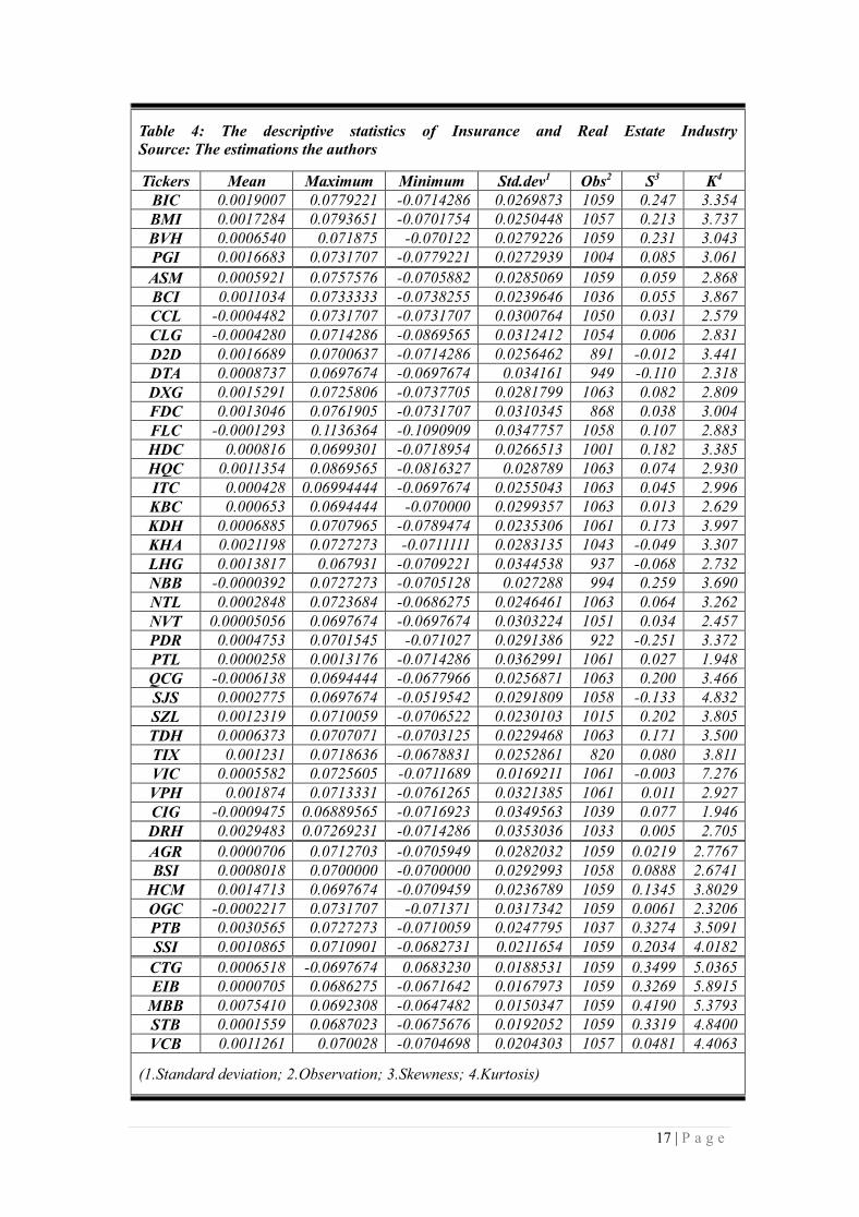
During the collected periods, the mean return of the insurance group is about

0.11488% while the mean return of the real estate is approximately 0.0709%. And the

mean return of the diversifed financial industry is 0.1044% and 1.1909% for banks

industry (see table 4)

Besides, the kurtosis and the skewness are used to show the form of distribution

of return. The “kurtosis” describe the degree of the peak of the distribution when the

“skewness” describe the asymmetric from the normal distribution. For normal

distribution, the skewness is equal to zero and the kurtosis is equal to three (excess

kurtosis equals zero). If the skewness is different from zero showing the

nonsymmetrical distribution when one side of the distribution does not mirror the other.

Particularly, the positive skewness indicates long right tail distribution which specifies

frequent small negative outcomes; when the negative skewness signs the long left tail

distribution which indicates a greater chance of extremenly negative scenarios.

Additionally, if it is the higher positive excess kurtosis (leptokurtosis) showing a higher

peak with fat tail than the normal distribution. The lower negative excess kurtosis

(platykurtosis) showing a lower peak with thin tail than normal (Ruey S.Tsay, 2005,

“Analsysis of Financial Time Series”, p.7-16).

According to the above descriptive statistic (see table 4 & 5), it shows that most

return series have not normal distribution. For insurance group, all stocks return have

the over-three kurtosis and positive non-zero skewness while for real estate, half of

them have over-three kurtosis and half have the lower-three kurtosis. Moreover, real

estate shows that seven stocks return have negative non-zero skewness and the

remainers have the postive skewness. For diversified financial industry, all stocks

return haave positive non-zero skewness; four lower-3-kurtosis tickers and two over-

12 | P a g e

3-kurtosis tickers. About banking group, the result shows that all had over-three

kurtosis and positive non-zero skewness.

To the four market-weighted indexes, all have over-three kurtosis and negative

skewness. Negative skewness signs the long left tail distribution which indicates a

greater chance of extremenly negative scenarios. And the higher positive excess

kurtosis (leptokurtosis) showing a higher peak with fat tail than the normal distribution.

In brief, for descriptive summary, either the general financial industry or the four

market-weighted had non-normal distribution of return (see table 5)

Pretesting for Stationarity (see table 6.1 to 6.3): The ADF (Dickey-Fuller 1979)

will test the null hypothesis of nonstationary and the alternative hypothesis of

stationary. It will reject the null hypothesis if the absolute value of ADF test statistic

exceeds the absolute critical value at 1%, 5% or 10% significance level (Mohd.Aminul

Islam 2013; Nguyen Quang Dong 2012, p.524-528; Ruey S.Tsay 2005). The test as

following:

𝒓𝒕 = 𝒄𝒕 + 𝜷𝒓 + ∑ 𝜱𝒊∆𝒓𝒕−𝒊 + 𝒆𝒊

𝒑−𝟏

𝒊=𝟏

𝑯𝟎: 𝜷 = 𝟏

𝑯𝟏: 𝜷 < 𝟏

We denote the rt is the return series; while ct can be zero or constant, ∆𝑥𝑡−𝑖 is the

differced series of rt . The the ADF-test statistic is calculated as below:

𝑨𝑫𝑭 − 𝒕𝒆𝒔𝒕 = �̂� − 𝟏

𝒔𝒕𝒅(�̂�) ; �̂� 𝑖𝑠 𝑡ℎ𝑒 𝑙𝑒𝑎𝑠𝑡 𝑠𝑞𝑢𝑎𝑟𝑒𝑑 𝑒𝑠𝑡𝑖𝑚𝑎𝑡𝑒 𝑜𝑓 𝛽

As consequence, we can conculde that all sample result show the stationary (see table

6a, 6b & 6c). This is the fundamental for the following step of forecasting. The same

application in the others papers could be listed as Mohd.Aminul Islam 2013; Ahmed

Elsheikh M.Ahmed & Suliman Zakaria 2011; Rilker Gokbulut & Mehmet Pekkaya

2014; Dana Al.Najjar 2016; Sohail Chand, Shahid Kamal & Imran Ali 2012; Suliman

13 | P a g e

Zakaria & Peter Winker 2012; M.Tamilselvan & Shaik Mastan Vali 2016, Trilochan

Tripathy & Luis A.Gil-Alana 2015.

Pretesting for Heteroscedasticity (see table 7.1 to 7.3): The other

characteristics series are the heteroscedaticity which must be tested by Lagrange

Multiplier test (Engle, 1982). Additionally, one of the most important issue before

applying ARCH or GARCH models is to first examine the residuals for evidence of

heteroscedaticity by the Lagrange Multiplier Test proposed by Engle 1982 which

previously applied by Ahmed Alsheikh M.Ahmed & Suliman Zakaria 2011; Suliman

Zakaria & Peter Winker 2012; Rilker Gokbulut & Mehmet Pekkaya 2014; Sohail

Chand, Shahid Kamal & Imran Ali 2012; Afees A.Salisu & Ismail O.Fasanya 2012;

M.Tamilselvan & Shaik Mastan Vali 2016. We will obtain the residuals from the OLS

regression of mean equation then squared its as below:

𝒆𝒕𝟐 = 𝜶𝟎 + 𝜶𝟏𝒆𝒕−𝟏

𝟐 + ⋯ + 𝜶𝒒𝒆𝒕−𝒒𝟐 + 𝜺𝒕

The null hypothesis that there is no ARCH effect formulated as:

H0: α1 = α2 =…= αq = 0

H1: αi ≠ 0 (for at least one i= 1,2,…,q)

(Another form H1: α12+ α2

2+…+ αq2

>0)

If the value of LM test statistic (TR2) is greater than the critical value from the X2(q)

distibution or the coeffient of the lagged term is statistically significant, the null

hypothesis will be rejected. The same conclusion can be achieved of the F-version of

the test is considered. As consequence, we get all the value of LM test of all research

sample showing that there is ARCH effect in the squared error

Pretesting the autocorrelation in residual (see table 8.1 to 8.3): According to

intruction of Ruey S.Tsay in the book named “Analysis of Financial Time Series”

published by John Wiley and Sons 2005 (The 2nd edition, p.107-119), by

reinvestigating on the squared residual obtained by mean equation, we check out the

14 | P a g e

autocorrelation function (ACF – autocorrelation function or PACF – partial

autocorrelation function), if it is statically different from zero, the autocorrelation in

residuals is ascertained. As can be seen from the result of table 8.1-8.3, all sample show

that the error terms are autocorrelated

In summary, we find the evidence of stationary but existing the ARCH effect and

autocorraltion in residuals. It is also the principal condition to apply ARCH, GARCH

models.

The orders of ARCH and GARCH-type models will be discussed in the section

5.2 of methodology. It is the common way using ACF and PACF of squared errors to

specifying the order m of ARCH proposed by Ruey S.Tsay (2005, p.106-107). Tim

Bollerslev, in 1992, demonstrated that GARCH could be adapted by low orders such

as GARCH(1,1), GARCH(1,2) and GARCH(2,1) (T.Bollerslev, Ray Y.Chou 1992 and

Kroner, “ARCH modelling in finance: A reivew of the theory and empirical evidence”,

Journal of econometrics 52).

15 | P a g e

Table 1: The HOSE classification of Financial industry (Insurance & Real Estate)

Source: Ho Chi Minh Stock Exchange – HOSE

Industry Tickers Name

Insurance

BIC The Vietnam Investment & Development Banking Insurance Co.

BMI Bao Minh J.S Company

BVH Bao Viet Insurance Corporation

PGI Petrolimex J.S Company

Rea

l es

tate

ASM Sao Mai J.S Company

BCI Binh Chanh Investment & Construction J.S Company

CCL Cuu Long Investment & Development J.S Company

CIG Coma18 J.S Company

CLG Cotec Housing Investment and Devepment J.S Co.

D2D The Two Industrial Development J.S Company

DRH Dream House Investment J.S Company

DTA De Tam J.S Company

DXG Dat Xanh Real Estate Service & Construction J.S Co.

FDC Ho Chi Minh Foreign & Invest Development J.S Co.

FLC FLC Corporation J.S Company

HAR An Duong Thao Dien Commercial Real Estate Investment J.S

Company

HDC Ba Ria Vung Tau Housing Development J.S Company

HQC Hoang Quan Real Estate Commerce & Service J.S Company

ITC Housing Investment J.S Company

KBC Kinh Bac City Development J.S Company

KDH Khang Dien Housing Investment J.S Company

KHA Khanh Hoi Investment & Service J.S Company

LDG Long Dien Investment J.S Company

LHG Long hau J.S Company

NBB Nam Bay Bay Investment J.S Company

NLG Nam Long Investment J.S Company

NTL Tu Liem City Development J.S Company

NVT Ninh Van Bay Real Estate & Traveling J.S Company

PDR Phat Dat Real Estate Development J.S Company

PTL Petro City & Infrastructure Investment J.S Co.

QCG Quoc Cuong Gia Lai J.S Co.

SJS Song Da City & Industry Development J.S Co.

SZL Sonadezi Long Thanh J.S Co.

TDH Thu Duc House Development J.S Co.

TIX Tan Binh Export Import Service & Investment J.S Co.

VIC Vingroup J.S Co.

VPH Van Phat Hung J.S Co.

16 | P a g e

Table 2: The HOSE classification of Financial industry (Diversified financials & Bank)

Source: Ho Chi Minh Stock Exchange – HOSE

Industry Tickers Name

Diversified Financials

AGR Agribank Securities Joint – Stock Corporation

BSI Vietnam Invest & Development Banking Securities J.S

Co.

HCM Ho Chi Minh Securities J.S Co.

OGC Ocean Group J.S Co.

PTB Phu Tai J.S Co.

SSI Sai Gon Securities J.S Co.

Banks

CTG Viet Nam Industrial Commerce J.S Bank

EIB Viet Nam Ex-Im J.S Bank

MBB Military J.S Bank

STB Sai Gon Commercial Trust J.S Bank

VCB Viet Nam Foreign Commerce J.S Bank

Table 3: The four market-weighted indexes

Source: HOSE, HNX

VNindex Hochiminh Stock Exchange Index

HNXindex Hanoi Stock Exchange Index

VN30 index The 30 largest capicalilation companies index

UPCOM index Unlisted Public Company Market Index

17 | P a g e

Table 4: The descriptive statistics of Insurance and Real Estate Industry

Source: The estimations the authors

Tickers Mean Maximum Minimum Std.dev1 Obs2 S3 K4

BIC 0.0019007 0.0779221 -0.0714286 0.0269873 1059 0.247 3.354

BMI 0.0017284 0.0793651 -0.0701754 0.0250448 1057 0.213 3.737

BVH 0.0006540 0.071875 -0.070122 0.0279226 1059 0.231 3.043

PGI 0.0016683 0.0731707 -0.0779221 0.0272939 1004 0.085 3.061

ASM 0.0005921 0.0757576 -0.0705882 0.0285069 1059 0.059 2.868

BCI 0.0011034 0.0733333 -0.0738255 0.0239646 1036 0.055 3.867

CCL -0.0004482 0.0731707 -0.0731707 0.0300764 1050 0.031 2.579

CLG -0.0004280 0.0714286 -0.0869565 0.0312412 1054 0.006 2.831

D2D 0.0016689 0.0700637 -0.0714286 0.0256462 891 -0.012 3.441

DTA 0.0008737 0.0697674 -0.0697674 0.034161 949 -0.110 2.318

DXG 0.0015291 0.0725806 -0.0737705 0.0281799 1063 0.082 2.809

FDC 0.0013046 0.0761905 -0.0731707 0.0310345 868 0.038 3.004

FLC -0.0001293 0.1136364 -0.1090909 0.0347757 1058 0.107 2.883

HDC 0.000816 0.0699301 -0.0718954 0.0266513 1001 0.182 3.385

HQC 0.0011354 0.0869565 -0.0816327 0.028789 1063 0.074 2.930

ITC 0.000428 0.06994444 -0.0697674 0.0255043 1063 0.045 2.996

KBC 0.000653 0.0694444 -0.070000 0.0299357 1063 0.013 2.629

KDH 0.0006885 0.0707965 -0.0789474 0.0235306 1061 0.173 3.997

KHA 0.0021198 0.0727273 -0.0711111 0.0283135 1043 -0.049 3.307

LHG 0.0013817 0.067931 -0.0709221 0.0344538 937 -0.068 2.732

NBB -0.0000392 0.0727273 -0.0705128 0.027288 994 0.259 3.690

NTL 0.0002848 0.0723684 -0.0686275 0.0246461 1063 0.064 3.262

NVT 0.00005056 0.0697674 -0.0697674 0.0303224 1051 0.034 2.457

PDR 0.0004753 0.0701545 -0.071027 0.0291386 922 -0.251 3.372

PTL 0.0000258 0.0013176 -0.0714286 0.0362991 1061 0.027 1.948

QCG -0.0006138 0.0694444 -0.0677966 0.0256871 1063 0.200 3.466

SJS 0.0002775 0.0697674 -0.0519542 0.0291809 1058 -0.133 4.832

SZL 0.0012319 0.0710059 -0.0706522 0.0230103 1015 0.202 3.805

TDH 0.0006373 0.0707071 -0.0703125 0.0229468 1063 0.171 3.500

TIX 0.001231 0.0718636 -0.0678831 0.0252861 820 0.080 3.811

VIC 0.0005582 0.0725605 -0.0711689 0.0169211 1061 -0.003 7.276

VPH 0.001874 0.0713331 -0.0761265 0.0321385 1061 0.011 2.927

CIG -0.0009475 0.06889565 -0.0716923 0.0349563 1039 0.077 1.946

DRH 0.0029483 0.07269231 -0.0714286 0.0353036 1033 0.005 2.705

AGR 0.0000706 0.0712703 -0.0705949 0.0282032 1059 0.0219 2.7767

BSI 0.0008018 0.0700000 -0.0700000 0.0292993 1058 0.0888 2.6741

HCM 0.0014713 0.0697674 -0.0709459 0.0236789 1059 0.1345 3.8029

OGC -0.0002217 0.0731707 -0.071371 0.0317342 1059 0.0061 2.3206

PTB 0.0030565 0.0727273 -0.0710059 0.0247795 1037 0.3274 3.5091

SSI 0.0010865 0.0710901 -0.0682731 0.0211654 1059 0.2034 4.0182

CTG 0.0006518 -0.0697674 0.0683230 0.0188531 1059 0.3499 5.0365

EIB 0.0000705 0.0686275 -0.0671642 0.0167973 1059 0.3269 5.8915

MBB 0.0075410 0.0692308 -0.0647482 0.0150347 1059 0.4190 5.3793

STB 0.0001559 0.0687023 -0.0675676 0.0192052 1059 0.3319 4.8400

VCB 0.0011261 0.070028 -0.0704698 0.0204303 1057 0.0481 4.4063

(1.Standard deviation; 2.Observation; 3.Skewness; 4.Kurtosis)

18 | P a g e

Table 5: The descriptive statistics of the four market-weighted indexes

Source: The estimations the authors

Tickers Mean Maximum Minimum Std.dev1 Obs2 S3 K4

Vnindex 0.0004643 0.0392557 -0.0605465 0.0112674 1059 -0.5596313 5.501443

HNXindex 0.0003258 0.0556075 -0.064800 0.0127936 1059 -0.540226 5.992988

VN30 0.0003941 0.0416241 -0.0577473 0.0112687 1060 -0.4343574 5.474966

UPCOM 0.0005316 0.0742958 -0.0644823 0.0111791 1059 -0.1658537 14.52935

19 | P a g e

Table 6.1: Dickey-Fuller test of stationary for Insurance and Real Estate

Industry

Source: The estimation of authors

Tickers Test Statistic

Z(t) 1% level 5% level 10% level

BIC -30.926 -3.430 -2.860 -2.570

BMI -32.845 -3.430 -2.860 -2.570

BVH -29.435 -3.430 -2.860 -2.570

PGI -38.553 -3.430 -2.860 -2.570

ASM -30.115 -3.430 -2.860 -2.570

BCI -31.552 -3.430 -2.860 -2.570

CCL -31.074 -3.430 -2.860 -2.570

CIG -29.892 -3.430 -2.860 -2.570

D2D -38.416 -3.430 -2.860 -2.570

DRH -28.163 -3.430 -2.860 -2.570

DTA -28.035 -3.430 -2.860 -2.570

DXG -30.062 -3.430 -2.860 -2.570

FDC -29.644 -3.430 -2.860 -2.570

FLC -30.012 -3.430 -2.860 -2.570

HDC -36.813 -3.430 -2.860 -2.570

HQC -31.190 -3.430 -2.860 -2.570

ITC -32.189 -3.430 -2.860 -2.570

KBC -31.597 -3.430 -2.860 -2.570

KDH -30.117 -3.430 -2.860 -2.570

KHA -44.270 -3.430 -2.860 -2.570

LHG -32.622 -3.430 -2.860 -2.570

NBB -30.991 -3.430 -2.860 -2.570

NTL -30.948 -3.430 -2.860 -2.570

NVT -31.269 -3.430 -2.860 -2.570

PDR -31.287 -3.430 -2.860 -2.570

PTL -33.009 -3.430 -2.860 -2.570

QCG -30.893 -3.430 -2.860 -2.570

SJS -28.641 -3.430 -2.860 -2.570

SZL -35.677 -3.430 -2.860 -2.570

TDH -29.447 -3.430 -2.860 -2.570

TIX -36.731 -3.430 -2.860 -2.570

VIC -33.915 -3.430 -2.860 -2.570

VPH -31.781 -3.430 -2.860 -2.570

20 | P a g e

Table 6.2: Dickey-Fuller test of Stationarity for Diversified finance and Banks


Tickers Test statistic

Z(t)

1% Critical

value

5% Critical

value

10%

Critical

value

P-value for

Z(t)

AGR -33.954 -3.430 -2.860 -2.570 0.000

BSI -30.455 -3.430 -2.860 -2.570 0.000

HCM -31.368 -3.430 -2.860 -2.570 0.000

OGC -30.327 -3.430 -2.860 -2.570 0.000

PTB -32.681 -3.430 -2.860 -2.570 0.000

SSI -32.869 -3.430 -2.860 -2.570 0.000

CTG -32.367 -3.430 -2.860 -2.570 0.000

EIB -29.909 -3.430 -2.860 -2.570 0.000

MBB -34.659 -3.430 -2.860 -2.570 0.000

STB -29.979 -3.430 -2.860 -2.570 0.000

VCB -31.725 -3.430 -2.860 -2.570 0.000

Table 6.3: Pretest of Stationarity for Vnindex, HNXindex, VN30index, UPCOMindex


Tickers Test statistic 1% Critical

value

5% Critical

value

10% Critical

value

P-value

VNindex -30.417 -3.439 -2.860 -2.571 0.00000

HNXindex -33.373 -3.340 -2.860 -2.570 0.00000

VN30index -30.464 -3.430 -2.860 -2.570 0.00000

UPCOMindex -18.852 -3.420 -2.830 -2.570 0.00000

21 | P a g e

Table 7.1: Pre-estimation of heteroscedasticity for Insurance and Real Estate

Industry

Source: Estimated by the authors

Tickers LM test statistic P-value

BIC 106.474 0.00000

BMI 40.354 0.00000

BVH 150.515 0.00000

PGI 38.153 0.00000

ASM 41.592 0.00000

BCI 54.639 0.00000

CCL 61.987 0.00000

CIG 79.241 0.00000

CLG 112.242 0.00000

D2D 66.681 0.00000

DRH 71.523 0.00000

DTA 71.741 0.00000

DXG 32.385 0.00000

FDC 123.424 0.00000

FLC 58.442 0.00000

HDC 38.913 0.00000

HQC 37.659 0.00000

ITC 38.443 0.00000

KBC 59.228 0.00000

KDH 94.132 0.00000

KHA 104.797 0.00000

LHG 57.406 0.00000

NBB 106.293 0.00000

NTL 32.55 0.00000

NVT 40.173 0.00000

PDR 92.299 0.00000

PTL 36.19 0.00000

QCG 83.189 0.00000

SJS 68.075 0.00000

SZL 37.714 0.00000

TDH 49.02 0.00000

TIX 85.908 0.00000

VIC 11.401 0.00070

VPH 6.855 0.00880

22 | P a g e

Table 7.2: Pre-estimation of heteroscedasticity for Diversified finance and Banks

Source: The estimation of author

Tickers L-M test statistic P-value

AGR 75.370 0.000

BSI 28.925 0.000

HCM 45.606 0.000

OGC 22.285 0.000

PTB 66.774 0.000

SSI 16.473 0.000

CTG 43.306 0.000

EIB 144.625 0.000

MBB 20.998 0.000

STB 123.713 0.000

VCB 18.074 0.000

Table 7.3: Pretest of Heteroscedasticity for VNindex, HNXindex, VN30 index and UPCOM

index


Tickers Lagrange Multiplier test statistic P-value

VNindex 15.794 0.00010

HNXindex 29.166 0.00000

VN30index 16.681 0.00000

UPCOMindex 449.943 0.00000

23 | P a g e

Table 8.1: Pretest of autocorrelation in squared error for Insurance and real estate


Tickers AC PAC Q statisitc Prob

BIC 0.3171 0.3172 106.79 0.00000

BMI 0.1954 0.1955 40.487 0.00000

BVH 0.3771 0.3771 151.00 0.00000

PGI 0.1950 0.1951 38.286 0.00000

ASM 0.1982 0.1983 41.717 0.00000

BCI 0.2292 0.2293 54.600 0.00000

CCL 0.2430 0.2431 62.157 0.00000

CIG 0.2761 0.2764 79.455 0.00000

CLG 0.3264 0.3266 112.61 0.00000

D2D 0.2737 0.2737 66.948 0.00000

DRH 0.2631 0.2632 71.687 0.00000

DTA 0.2751 0.2751 72.026 0.00000

DXG 0.1746 0.1746 32.495 0.00000

FDC 0.3771 0.3773 123.86 0.00000

FLC 0.2350 0.2352 58.614 0.00000

HDC 0.1972 0.1973 39.041 0.00000

HQC 0.1882 0.1883 37.765 0.00000

ITC 0.1902 0.1903 38.569 0.00000

KBC 0.2361 0.2361 59.407 0.00000

KDH 0.2979 0.2979 94.397 0.00000

KHA 0.3170 0.3171 105.13 0.00000

LHG 0.2474 0.2474 57.548 0.00000

NBB 0.3268 0.3268 106.46 0.00000

NTL 0.1739 0.1762 32.245 0.00000

NVT 0.1955 0.1956 40.274 0.00000

PDR 0.3163 0.3165 92.558 0.00000

PTL 0.1846 0.1848 36.255 0.00000

QCG 0.2797 0.2798 83.373 0.00000

SJS 0.2537 0.2538 68.31 0.00000

SZL 0.1928 0.1928 37.848 0.00000

TDH 0.2148 0.2148 49.189 0.00000

TIX 0.3238 0.3238 86.282 0.00000

VIC 0.1037 0.1037 11.442 0.00007

VPH 0.1084 0.1085 6.878 0.00870

24 | P a g e

Table 8.2: Pretest of autocorrelation in squared error for Diversified finance and

banks



AGR 0.2653 0.2679 74.771 0.00000

BSI 0.1653 0.1654 29.005 0.00000

HCM 0.2076 0.2076 45.760 0.00000

OGC 0.1451 0.1451 22.369 0.00000

PTB 0.2538 0.2539 66.979 0.00000

SSI 0.1248 0.1248 16.530 0.00000

CTG 0.2015 0.2016 43.126 0.00000

EIB 0.3697 0.3697 145.16 0.00000

MBB 0.1409 0.1409 21.07 0.00000

STB 0.3415 0.3416 123.88 0.00000

VCB 0.1308 0.1308 18.136 0.00000

Table 8.3: Pretest of autocorrelation in squared error for the hour market-

weighted indexes

Source: The estimation authors


Vnindex 0.1222 0.1222 15.848 0.0001

HNXindex 0.1660 0.1660 29.271 0.0000

VN30 index 0.1255 0.1255 16.738 0.0000

UPCOM index 0.6521 0.6521 451.58 0.0000

25 | P a g e

4.2. Methodology

Conditional heteroscedastic models are the basic econometrics tools used to

estimate and forecast asset return volatility depending on each time-series

characteristics. In the section we will review both symmetric (ARCH, GARCH) and

asymmetric GARCH-type models (EGARCH, GJRGARCH). Our aims are to study

some statistical methods and econommetric models avaible in the literature for

modelling the conditional heteroscedastic volatility model.

The univariate volatility models include the autoregressive conditional

heteroscedastic (ARCH) model of Engle (1982), the generalized ARCH (GARCH)

model of Bollerslev (1986), GARCH-in-mean of Engle, Lilien and Robin (1987), the

exponential GARCH (EGARCH) model of Nelson (1991), the GJRGARCH model of

Glosten, Jagannathan & Runkle (1993). These are models which will be displayed in

our current paper using the information selection criteria (AIC and BIC) to choose the

best fit. Following Ching Mun Lim & Siok Kun Sek (2013), we assume that the

conditional mean equation of stock return is defined as the constant term plus residuals

term: rt = μ + εt.

4.2.1. ARCH (m) – Engle 1982

Ruey S.Tsay in 2005 gave some instructions of model building with four phase:

specifying the mean equation and obtaining the residuals; conducting ARCH effect test

on the obtained residuals, the third with ARCH/GARCH model estimationand last step

of careful checking the fittest model and refining if necessary. The general model of

ARCH (m) process is as follow (Engle, 1982):

𝒓𝒕 = 𝝁 + 𝒖𝒕

𝒖𝒕 = 𝝈𝒕𝜺𝒕

𝝈𝒕𝟐 = 𝜱𝟎 + 𝜱𝟏𝒖𝒕−𝟏

𝟐 + ⋯ + 𝜱𝒎𝒖𝒕−𝒎𝟐

𝝈𝒕𝟐 = 𝜱𝟎 + ∑ 𝜱𝒊

𝒎

𝒊=𝟏

𝒖𝒕−𝒊𝟐

(𝜱𝟎 > 𝟎, 𝜱𝒊 ≥ 𝟎 𝒇𝒐𝒓 𝒊 > 𝟎)

Where Φ0 is constant, бt2 is the squared conditional variance of error term, ut-m

is the lagged value of error term. In general, бt2 is expressed as a function of past

squared errors. Another issue is that the unknown coefficients (Φ0, Φ1, Φ2,… Φm) must

26 | P a g e

be non-negative since the variance can not be negative meaning that ARCH assume

that positive and negative shocks have the same effects on volatility because it depends

on the squared of previous shocks. However the asymmetric literature proved that

return of financial asset responds differently to either positive or negative shocks (Ruey

S.Tay 2005; Nelson 1991; Glosten, Jagannathan and Runkle 1993 and Zakoian 1994;

Ding, Granger and Engle 1993).

If these coefficient are positive and the recent squared residual are large, ARCH

predicts that the current squared error will be large in magnitude in the sense that its

variance is large. Hence, ARCH models are likely to overpredict the volatility because

they respond slowly to large isolated shocks to return series (Ruey S.Tay 2005).

And if the ARCH effect is found to be statistically significant, we can use PACF

of ut2 (squared error term specified by correlogram in Stata programme) to intepret the

ARCH order (m). We have:

бt2 = Φ0 + Φ1u2

t-1 + Φ2 u2t-2 + … +Φm u2

t-m

Hence, u2t is an unbiased estimate of the squared variance of error term

(бt2).Otherwise, it is expected that u2

t is the linear regression of u2t-1, u2

t-2,…,u2t-m

as same as the autoregressive function AR(q) when the PACF is the useful tool for

determing the order of AR(q). For AR(q) model, the lagged (1) sample of PACF will

be close to zero. In brief, for an AR(q) series, the sample PACF cuts off at lag q and

the same version for ARCH(m) model based on PACF of squared errors (Ruey S.Tay

2005).

However, ARCH models are likely to overpredict the volatility since they

respond slowly to large shocks to the return. Additionally, ARCH(m) estimation will

often require a large number of parameters and higher order m to capture the volatility

process. As consequence, to remedy this problem, Bollerslev 1986 developed the

Generalized ARCH model (GARCH).

27 | P a g e

4.2.2. GARCH (m,s) - Bollerslev 1986

The standard GARCH (m,s) model espresses the variance at time t as following:

𝒓𝒕 = 𝝁 + 𝒖𝒕 𝒖𝒕 = 𝝈𝒕𝜺𝒕

𝝈𝒕𝟐 = 𝜱𝟎 + ∑ 𝜱𝒊

𝒎

𝒊=𝟏

𝒖𝒕−𝒊𝟐 + ∑ 𝜽𝒋

𝒔

𝒋=𝟏

𝝈𝒕−𝒋𝟐

[ 𝜱𝟎 > 𝟎, 𝜱𝒊 & 𝜽𝒋 ≥ 𝟎, ∑ (

𝒎𝒂𝒙(𝒎.𝒔)

𝒊=𝟏

𝜱𝒊 + 𝜽𝒋) < 𝟏 ]

The GARCH model allows the error variance (б2t) depending on either its own

past squared errors (u2t-m) or its own past values (б2

t-s) where m is the order of ARCH

terms and s is the order of GARCH term. GARCH also assumes that the variance is

non-negative. Large s order signs that shocks to the conditional variance take a long

time to die out meaning highly persistent volatility while large m order implies a

sizeable reaction of volatility to market movement. Hence, if 𝜱𝒊 + 𝜽𝒋 is close to untity,

the shock at t time will be persistent for many future periods. And one of the weakness

of GARCH model is the asumption of symmetry in volatility estimation.

We will apply GARCH(1,1), GARCH(1,2) and GARCH(2,1) with low order to

model the volatility and then use the information criteria to select the best fit (Ruey

S.Tsay 2005). Tim Bollerslev, in 1992, also specified that most low order GARCH such

as GARCH(1,1), GARCH(1,2) or GARCH(2,1) were employed (Tim Bollerslev, Ray

Y.Chou, Kenneth F.Kroner, “ARCH modeling in finance- A review of theory and

empirical evidence”, Journal of econometrics 52 (100), 1992, p.21-22).

4.2.3. GARCH-in-mean (m,s) – Engle, Lilien and Robin (1987)

Engle assume that the return of a security my depend on its volatility. To model

such a phenomenon, GARCH-in-mean was introduced with the following model:

𝒓𝒕 = 𝝁 + 𝒖𝒕 + 𝒄𝝈𝒕𝟐


𝝈𝒕𝟐 = 𝜱𝟎 + ∑ 𝜱𝒊

𝒎

𝒊=𝟏

𝒖𝒕−𝒊𝟐 + ∑ 𝜽𝒋

𝒔

𝒋=𝟏

𝝈𝒕−𝒋𝟐

28 | P a g e

The parameter c is called the risk premium parameter. The term of variance 𝝈𝒕𝟐

is added into the conditional mean equation intepreting the risk-return tradeoff

hypothesis. As an application, it can be listed such as Mohd.Aminul Islam 2013,

Suliman Zakaria & Peter Winkers 2012, Ahmed Elsheikh & Suliam Zakaria 2011.

If the parameter c is statistically positive, it will confirm the positive relationship

between return and volatility meaning high risk – high return. In order words, an

increase in return is caused by an increasse in the conditional variance (Enders, 2004,

“Applied Econometric Time Series, 2nd edition, Wiley Series in Probability and

Statistics). But either GARCH or GARCH-in-mean are also considered to be

symmetric model assuming that both positive and negative shocks of equal size

generate an equal effect on volatility.

Nonetheless, the negative shocks tend to have a larger impact on future volatility

than the positive one, namely asymmetric or leverage effect which has to be captured

by others asymmetric GARCH models (for instance: Exponential GARCH model

(EGARCH) of Nelson 1991 and GJRGARCH model of Glosten, Jagannathan and

Runkle 1993 as following sections).

4.2.4. Exponential GARCH (EGARCH) – Nelson 1991

To remedy some weakness of symmetric GARCH model, Nelson advanced the

following model as: EGARCH(m,s):

𝒓𝒕 = 𝝁 + 𝒖𝒕


𝒍𝒏(𝝈𝒕𝟐) = 𝜱𝟎 + ∑ 𝜱𝒊

𝒔

𝒊=𝟏

|𝒖𝒕−𝒊| + 𝜸𝒊𝒖𝒕−𝒊

𝝈𝒕−𝒊+ ∑ 𝜽𝒋

𝒎

𝒋=𝟏

𝒍𝒏 (𝝈𝒕−𝒋𝟐 )

The presence of parameter 𝜸𝒊 indicates an asymmetric effect of shocks on

volatility and the value of is statistically different from zero or negative signing the

asymmetry or the leverage effect (Ruey S.Tsay 2005; R.Ilker Gokbulut & Mehmet

Pekkaya 2014; Mohd.Aminul Islam 2013; M.Tamiselvan & Shaik Mastan Vali 2016;

Suliman Zakaria & Peter Winker 2012; Dana Al.Najjar 2016). Nelson used the logged

conditional variance to relax the positiveness contraint of GARCH model (Ruey S.Tsay

2005) and applied the absolute value of 𝒖𝒕−𝒊 to respond asymmetrically to positive

and negative lagged value of ut .

29 | P a g e

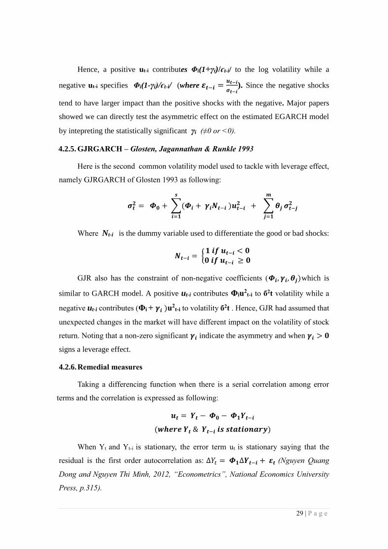
Hence, a positive ut-i contributes Φi(1+γi)/єt-i/ to the log volatility while a

negative ut-i specifies Φi(1-γi)/єt-i/ (where 𝜺𝒕−𝒊 =𝒖𝒕−𝒊

𝝈𝒕−𝒊). Since the negative shocks

tend to have larger impact than the positive shocks with the negative. Major papers

showed we can directly test the asymmetric effect on the estimated EGARCH model

by intepreting the statistically significant γi (≠0 or <0).

4.2.5. GJRGARCH – Glosten, Jagannathan & Runkle 1993

Here is the second common volatility model used to tackle with leverage effect,

namely GJRGARCH of Glosten 1993 as following:

𝝈𝒕𝟐 = 𝜱𝟎 + ∑(𝜱𝒊 + 𝜸𝒊𝑵𝒕−𝒊 )𝒖𝒕−𝒊

𝟐

𝒔

𝒊=𝟏

+ ∑ 𝜽𝒋

𝒎

𝒋=𝟏

𝝈𝒕−𝒋𝟐

Where Nt-i is the dummy variable used to differentiate the good or bad shocks:

𝑵𝒕−𝒊 = {𝟏 𝒊𝒇 𝒖𝒕−𝒊 < 𝟎𝟎 𝒊𝒇 𝒖𝒕−𝒊 ≥ 𝟎

GJR also has the constraint of non-negative coefficients (𝜱𝒊, 𝜸𝒊, 𝜽𝒋)which is

similar to GARCH model. A positive ut-i contributes Φiu2t-i to б2t volatility while a

negative ut-i contributes (Φi + 𝜸𝒊 )u2t-i to volatility б2t . Hence, GJR had assumed that

unexpected changes in the market will have different impact on the volatility of stock

return. Noting that a non-zero significant 𝜸𝒊 indicate the asymmetry and when 𝜸𝒊 > 𝟎

signs a leverage effect.

4.2.6. Remedial measures

Taking a differencing function when there is a serial correlation among error

terms and the correlation is expressed as following:

𝒖𝒕 = 𝒀𝒕 − 𝜱𝟎 − 𝜱𝟏𝒀𝒕−𝒊

(𝒘𝒉𝒆𝒓𝒆 𝒀𝒕 & 𝒀𝒕−𝒊 𝒊𝒔 𝒔𝒕𝒂𝒕𝒊𝒐𝒏𝒂𝒓𝒚)

When Yt and Yt-i is stationary, the error term ut is stationary saying that the

residual is the first order autocorrelation as: ∆𝑌𝑡 = 𝜱𝟏∆𝒀𝒕−𝒊 + 𝜺𝒕 (Nguyen Quang

Dong and Nguyen Thi Minh, 2012, “Econometrics”, National Economics University

Press, p.315).

30 | P a g e

Normally, the economic time series, such as stock return series would deal with

autocorrelation in residuals resulting the autorrelation function value often exceeds

zero (detected by ACF and PACF functions). Denoting the autocorrelation function

ACF(k) is ρk (Ruey S.Tsay, 2005, p.25-30):

𝝆𝒌 = 𝒄𝒐𝒓𝒓(𝒀𝒕, 𝒀𝒕−𝒌) = 𝜹𝒌

𝜹𝟎, 𝒌 = 𝟎, 𝟏, 𝟐, …

𝒘𝒉𝒆𝒓𝒆 𝜹𝒌 = 𝒄𝒐𝒗(𝒀𝒌, 𝒀𝒕−𝒌), 𝒌 = 𝟎, 𝟏, 𝟐, …

𝒘𝒉𝒆𝒏 𝒌 = 𝟎, 𝜹𝟎 = 𝒗𝒂𝒓(𝒀𝒕 )

(𝒔𝒆𝒆 𝒀𝒕 𝒂𝒔 𝒆𝒓𝒓𝒐𝒓 𝒕𝒆𝒓𝒎 𝒖𝒕)

4.2.7. Autocorrelation

Noting that serial correlation is related to the variance of parameter and if, after

model estimation, there is still correlated we should reject that models. Now we have

the equation of parameter variance, perhaps homoscedasticity is satisfied (Nguyen

Quang Dong, 2012):

𝒗𝒂𝒓(𝜷�̂�) = 𝝈𝟐

∑ 𝒙𝟐𝒕𝟐

𝒕

+ 𝟐 ∑ ∑ 𝒌𝒕𝒌𝒕+𝒔𝒄𝒐𝒗(𝒖𝒕, 𝒖𝒕+𝒔)

𝒏−𝒕

𝒔=𝟏

𝒏

𝒕=𝟏

Hence, when there is autocorrelated residuals, 𝟐 ∑ ∑ 𝒌𝒕𝒌𝒕+𝒔𝒄𝒐𝒗(𝒖𝒕, 𝒖𝒕+𝒔)𝒏−𝒕𝒔=𝟏

𝒏𝒕=𝟏 will

be different from zero causing that the variance of estimated parameter will be biased.

We could not continuously adapt the models and then the remedial measure of

diiferencing and loggeg function is to be used (as discussed in section 5.2.6).

4.2.8. Model information criteria

Akaike (1973) proposed AIC (Akaike information criteria) for model selection

(ARIMA, GARCHs) denoted as following:

𝑨𝑰𝑪(𝒍) = 𝐥𝐧 (𝝈𝒍𝟐)̂ +

𝟐𝒍

𝑻

𝒘𝒉𝒆𝒓𝒆 𝑻 𝒊𝒔 𝒔𝒂𝒎𝒑𝒍𝒆 𝒔𝒊𝒛𝒆 & 𝒍 𝒊𝒔 𝒕𝒐𝒕𝒂𝒍 𝒐𝒓𝒅𝒆𝒓

& 𝝈𝒍�̂� 𝒊𝒔 𝒕𝒉𝒆 𝒎𝒂𝒙𝒊𝒎𝒖𝒎 𝒍𝒊𝒌𝒆𝒍𝒊𝒉𝒐𝒐𝒅 𝒆𝒔𝒕𝒊𝒎𝒂𝒕𝒆 𝒐𝒇 𝝈𝒍

𝟐

𝝈𝒍𝟐 𝒊𝒔 𝒕𝒉𝒆 𝒄𝒐𝒏𝒅𝒊𝒕𝒊𝒐𝒏𝒂𝒍 𝒗𝒂𝒓𝒊𝒂𝒏𝒄𝒆 𝒐𝒇 𝒖𝒕

The first phrase of AIC measures the goodness of fit and the second phrase expressed

as the penalty function of the criterion. And Schwarz Bayesian (1978) introduced

another criteria (BIC):

31 | P a g e

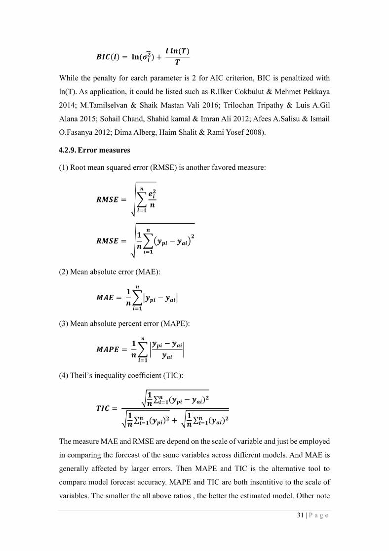
𝑩𝑰𝑪(𝒍) = 𝐥𝐧 (𝝈𝒍𝟐)̂ +

𝒍 𝒍𝒏(𝑻)

𝑻

While the penalty for earch parameter is 2 for AIC criterion, BIC is penaltized with

ln(T). As application, it could be listed such as R.Ilker Cokbulut & Mehmet Pekkaya

2014; M.Tamilselvan & Shaik Mastan Vali 2016; Trilochan Tripathy & Luis A.Gil

Alana 2015; Sohail Chand, Shahid kamal & Imran Ali 2012; Afees A.Salisu & Ismail

O.Fasanya 2012; Dima Alberg, Haim Shalit & Rami Yosef 2008).

4.2.9. Error measures

(1) Root mean squared error (RMSE) is another favored measure:

𝑹𝑴𝑺𝑬 = √∑𝒆𝒊

𝟐

𝒏

𝒏

𝒊=𝟏

𝑹𝑴𝑺𝑬 = √𝟏

𝒏∑(𝒚𝒑𝒊 − 𝒚𝒂𝒊)

𝟐𝒏

𝒊=𝟏

(2) Mean absolute error (MAE):

𝑴𝑨𝑬 = 𝟏

𝒏∑|𝒚𝒑𝒊 − 𝒚𝒂𝒊|

𝒏

𝒊=𝟏

(3) Mean absolute percent error (MAPE):

𝑴𝑨𝑷𝑬 = 𝟏

𝒏∑ |

𝒚𝒑𝒊 − 𝒚𝒂𝒊

𝒚𝒂𝒊|

𝒏

𝒊=𝟏

(4) Theil’s inequality coefficient (TIC):

𝑻𝑰𝑪 =

√𝟏𝒏

∑ (𝒚𝒑𝒊 − 𝒚𝒂𝒊)𝟐𝒏𝒊=𝟏

√𝟏𝒏

∑ (𝒚𝒑𝒊)𝟐𝒏𝒊=𝟏 + √𝟏

𝒏∑ (𝒚𝒂𝒊)𝟐𝒏

𝒊=𝟏

The measure MAE and RMSE are depend on the scale of variable and just be employed

in comparing the forecast of the same variables across different models. And MAE is

generally affected by larger errors. Then MAPE and TIC is the alternative tool to

compare model forecast accuracy. MAPE and TIC are both insentitive to the scale of

variables. The smaller the all above ratios , the better the estimated model. Other note

32 | P a g e

that TIC is ranges between zero and one with the value of TIC converging to zero

showing the better. Heping Liu & Jing Shi 2013, Ching Mun Lim & Siok Kun Sek

2013 and Dima Alberg 2008 had applied these measure into their papers to compare

among defined symmetric and asymmetric volatility models. Hence, we just utilize the

MAPE and TIC to compare the model’s accuracy.

4.2.10. The l-step ahead forecast

The last phases came for forecasting with the l-step ahead forecast for ARCH(m) at the

forecast origin h (Ruey S.Tsay, 2005). The 1-step ahead forecast is denoted б2h+1:

𝝈𝒉𝟐(𝟏) = ɸ𝟎 + ɸ𝟏𝒖𝒉

𝟐 + ⋯ + ɸ𝒎𝒖𝒉+𝟏−𝒎𝟐

The 2-step ahead forecast б2h+2 :

𝝈𝒉𝟐(𝟐) = ɸ𝟎 + ɸ𝟏𝝈𝒉

𝟐(𝟏) + ɸ𝟐𝒖𝒉𝟐 + ⋯ + ɸ𝒎𝒖𝒉+𝟐−𝒎

𝟐

We have the general equation for l-step forecast as following:

𝝈𝒉𝟐(𝒍) = ɸ𝟎 + ∑ ɸ𝒊

𝒎

𝒊=𝟏

𝝈𝒉𝟐(𝒍 − 𝒊)

𝒘𝒉𝒆𝒓𝒆 𝝈𝒉𝟐(𝒍 − 𝒊) = 𝒖𝒉+𝒍−𝒊

𝟐 𝒘𝒊𝒕𝒉 (𝒍 − 𝒊 < 𝟎)

But we have to note that the weakness of ARCH models are likely to overpredict the

volatility because they respond slowly to large shock to return. GARCH also has others

shortcoming that the large past squared value of residual and variance give an increase

to the current variance. GARCH’s phenomenon showed that the large shock in the past

tended to be followed by another large shock (as volatility clustering). Additionally,

the 1-step ahead forecast of GARCH(1,1) at the forecast origin h, as following:

𝝈𝒉+𝟏𝟐 = ɸ𝟎 + ɸ𝟏𝒖𝒉

𝟐 + 𝜷𝟏𝝈𝒉𝟐

(𝑤ℎ𝑒𝑟𝑒 𝑢ℎ & 𝜎ℎ2 𝑎𝑟𝑒 𝑘𝑛𝑜𝑤𝑛 𝑎𝑡 𝑡ℎ𝑒 𝑡𝑖𝑚𝑒 ℎ)

In general, for l-step ahead forecast in GARCH model, we have:

𝝈𝒉𝟐(𝒍) = ɸ𝟎 + (ɸ𝟏 + 𝜷𝟏)𝝈𝒉

𝟐(𝒍 − 𝟏), 𝒍 > 𝟏

33 | P a g e

5. EMPIRICAL RESULTS AND DISCUSSIONS

` To again introduce, data mangement is performed by Stata 12 programme. After

we pre-test the return seires in the section 5.1, the result displays that there was ARCH

effect in the residual but stationary.

The following sections are divided into two sections: section 5.1-the model

estimation for the financial industry, section 5.2-the model estimation for the four

market-weighted indexes.

The model we applied are ARCH(m), GARCH(m,s), GARCH-M(m,s)

EGARCH(m,s), EGARCH-M(m,s), GJRGARCH(m,s) and GJRGARCH-M(m,s).

For both section 5.1 and 5.2, we estimate the proper model and the value of BIC

and AIC will be generated after each model estimation in order to compare which is

more available. In our paper, we only disclose the result after using the AIC and BIC

to filter (see appendix 1)

Each section will also include the first post-estimation of ARCH effect and

serial correlation using again Lagrange-Multilier and ACF, respectively basing the

preceeding filter result.

If there is still remaning the ARCH effect or autocorrelation in residuals meaning

useless inadequate model, reject it. To remedy, we have to refine the model by

differencing and natural logarithic functions. We, first, also have to generate the ARCH

effect test. Then redefining the model on remedied data (see appendix 2)

Last, the second post-estimation of ARCH effect and autocorrealtion must be

executed (see appendix 3). If the post-estimated model, again, can not capture the

ARCH effect or serial correlation, reject it. Last, the remainers which can totally

capture the ARCH effect and serial correlation are used to forecast. The error measures

will be generated to choose which is the best accuracy one.

34 | P a g e

5.1. The model estimation result of the financial industry

5.1.1.The model selection

After executing both symmetric and asymmetric GARCH, the two information

criterions (AIC & BIC) were used to select the model and the detailed model

parameters will be attached on the appendix 1 (Appendix 1: The model parameters

result of financial industry)

ARCH model estimation (see table 9): For insurance industry including BIC,

PGI, BMI and BVH, the first two tickers followed ARCH(1) while the last two follow

ARCH(3) and no one was available for ARCH(4) and ARCH(5).

For real estate including 30 common stocks, the majority were available for

lower order ARCH models (ARCH(1) and ARCH(2)). There were five tickers followed

ARCH(3) which were BCI, CLG, FLC, NTL, TDH and the last one ITC followed

ARCH(4). In short, most tickers in real estate followed the ARCH(1) & ARCH(2).

For diversified finance, three tickers followed ARCH(3) which were HCM, OGC,

SSI. The ARCH(1) was fitted by BSI and AGR was used for ARCH(2). Especially,

only one tickers followed ARCH(4) which was PTB.

Beside, banking tickers seemed to be available for high order ARCH, at least 2.

We had CTG and MBB following much high order ARCH(4) and ARCH(5).

Now we have to focus the principle of the ARCH’s weakness. ARCH model

often require many parameter to adequately describe the volatility process of return

series so that we other proper model was GARCH-family models. Our results seemed

to correspond with the previous papers, GARCH(1,1) was more available for most

tickers

GARCH-family models estimation (see table 10.1 – 10.2): The insurance

industry was totally captured by both symmetric and asymmetric GARCH(1,1). For

real estate, 16 tickers also followed the simplest model of GARCH and the others 14

tickers followed higher order. While most tickers in diversified finance and banking

group follow the lowest order GARCHs

Noting that, we can not applied these models if the post-estimation of

heteroscedasticity and autocorrelation test were not executed. And if the post results

indicated that they could not capture the problem, we have to refine the model by

35 | P a g e

differencing and logging functions.

5.1.2. The first postestimation of heteroscedasticity and autocorrelation

The test for conditional heteroscedasticity is the Lagrange multiplier (LM) test

proposed by Engle 1982. The test is equivalent to the F statistic for testing αi =0

(i=1,…,m) in this auxiliary linear regression (Ruey S.Tsay, “Analysis of financial time

series”, Second edition, page. 101-102). To retest whether there are any remaining

Arch Effect in the residuals, the LM test was also applied in R.Ilker Gokbulut &

Mehmet Pekkaya, 2014, “Estimating and forecasting volatility of financial markets

using Asymmetric Garch models: An application on Turkish financial markets”,

International Journal of Economics & Finance, vol.6, no.4, ISSN 1916-971X. Afees

A.Salisu & Ismail O.Fasanya in 2012 also conducted the ARCH LM test on order to

ascertain of the chosen models had captured these effects; the same as Kolade Sunday

Adesina.

Here below is the auxiliary regression of squared residual and its lagged value

on m lags which haved been previously selected using AIC and BIC information

criterion:

And the null hypothesis H0: α1=....=αm=0. First we have to obtain the residual and

square them. Then, we define the test statistic (TR2) and compare the p-value from this

statistic to the desired test level (α) and reject the null hypothesis if the p-value is

smaller (Ruey S.Tsay,” Analysis of financial time-series, Second edition, John Wiley

& Sons Publication, p.101-102).

Additionally, the autocorrelation of residuals have also been retested to confirm

whether there are any serial correlation by autocorrelation function of the obtained

squared residual from previous model selection phase (Ruey S.Tsay, “Analysis of

financial time-series”, Second edition, page. 116-120). The empirical test of

autocorrelation by ACF was also proposed by Walter Enders, “Applied Econometric

Time-Series”, John Wiley & Sons Publication, page.147-153.

If the both tests of heteroscedasticity and serial correlation in residuals show that

there is still remaining the ARCH effect or autocorrelation, the remedial measure

Tmtwhere

euuu tmtmtt

,...,1

... 22

110

2

36 | P a g e

including the log normal of return and differencing function must be applied (Nguyen

Quang Dong, “Econometrics”, 2012, page.295-317).

In term of application of autocorrelation retest, Haping Liu and Jing Shi in 2013

also employed the partial autocorrelation function (PACF) of residual to determine that

there did not exist significant autocorrelation among the residual gathered after each

model estimation. Their paper, in 2013, studied “Applying Arma-Garch approaches to

forecasting short-term electricity prices” which was published on the Journal of Energy

Economics p.152-166.

The result was unexpected. All of the four sub-industies was heteroscedastic

and serial corralted even if we applied both symmetric and asymmetric volatility

models (See table 11.1 to table 13.3). Table 11.1 to table 11.17 will present the first

post-test of ARCH effect and autocorrelation for insurance and real estate. Table 12.1

to table 12.3 will display the pre-test result of the diversified finance industry and table

13.1 to table 13.3 will display the result of banking industry.

There still existed a very high value of Chi squared distribution test and a zero

P-value much less than α (1%, 5% and 10%). As consequence, the null hypothesis of

no ARCH effect must be rejected. Other wise the test of autocorrelation also was

unsatisfactory as same as the ARCH effect result with a non-zero ACF and PACF and

p-value of zero much less than the α (1%, 5% or 10%).

This result was not satisfactory. Infact, this is an very important post-estimation

we have to execute. However, some researches ignored this phase such as Tran Manh

Tuyen, 2011, “Model volatility using GARCH models: Evidence from Vietnam”,

Economics Bulletin, Vol.31, no.3, pp.1935-1942. The lack of this postestimation was

also seen at the paper of Dana Al.Najjar, 2016 (Asian Journal of Finance & Accounting,

ISSN: 1946-052X, Vol8, No.1, p.152-167). The same inadequacy was signed at the

study of Shing Mun Lim & Siok Kun Sek, 2013 (Procedia Economics and Finance 5,

p.478-487) and of Dima Alberg, Haim Shalit and Rami Yosef, 2008 (Applied Financial

Economics 18, p.1201-1208).

37 | P a g e

Table 9: The first ARCH model classification for the Financial industry


Model Group Tickers

ARCH (1)

Insurance BIC, PGI

Real estate

D2D, DTA, FDC, HDC,

HQC, KHA, NVT, QCG, TIX,

VIC, VPH

Diverisified finance BSI

Bank None

ARCH(2)

Insurance None

Real estate

ASM, CCL, CIG, DXG,

DRH, KBC, KDH, LHG,

NBB, PDR, PTL, SJS, SZL.

Diverisified finance AGR

Bank STB, VCB

ARCH (3)

Insurance BMI, BVH

Real estate BCI, CLG, FLC, NTL, TDH

Diverisified finance HCM, OGC, SSI

Bank EIB

ARCH (4)

Insurance None

Real estate ITC

Diverisified finance PTB

Bank CTG

ARCH(5) Bank MBB

38 | P a g e

39 | P a g e

Table 10.1: The first symmetric and asymmetric GARCH classification for

insurance & real estate industries.


Models Group Tickers

Sym

met

ric

&

asy

mm

etri

c

GA

RC

H (

1,1

)

Insurance BIC, BMI, BVH, PGI

Real estate

ASM, BCI, CCL, CIG, CLG, DTA, FLC,

KBC, KDH, KHA, LHG, NBB, NVT, QCG,

SJS, SZL,

GARCH(1,2)

Real estate

FDC, ITC, PDR, D2D, DXG

GARCH-M(1,2) FDC, ITC, PDR, D2D, DXG,

GARCH(2,1) None

GARCH-M(2,1) None

EGARCH(1,2) FDC, HQC, NTL, D2D, DXG, VPH

EGARCH-M(1,2) TIX

EGARCH(2,1) None

EGARCH-M(2,1) HDC, PTL, TDH, VIC, DRH

GJRGARCH(1,2) FDC, ITC, PDR, D2D, DXG

GJRGARCH-M(1,2) FDC, ITC, PDR, DXG,

GJRGARCH(2,1) VPH

GJRGARCH-M(2,1) VPH

40 | P a g e

Table 10.2: The first symmetric and asymmetric GARCH estimation for

diversified & banking industries.


Models Group Tickers

Symmetric & asymmetric

GARCH (1,1)

Diverisified finance AGR, BSI, HCM, OGC,

PTB

Bank CTG, STB, MBB, VCB

EGARCH(1,2) Diverisified finance OGC

Bank MBB

EGARCH-M(2,1) Diverisified finance SSI

Bank EIB

GJRGARCH(2,1) Diverisified finance SSI

GJRGARCH-M(2,1) Diverisified finance SSI

Bank EIB

41 | P a g e

Table 11.1: The first postestimation of ARCH effect and Autocorrelation for

insurance


Tickers Lagrange Multiplier

test

Autocorrelation test

Chi-

squared

distribution

statistic

P-value AC PAC Q P-value

BIC

ARCH(1) 108.43402 0.00000 0.3200 0.3201 108.76 0.0000

GARCH

(1,1)

107.79909 0.00000 0.3191 0.3192 108.12 0.0000

GARCH-M

(1,1)

88.006431 0.00000 0.2883 0.2884 88.27 0.0000

EGARCH

(1,1)

107.4123 0.00000 0.3185 0.3186 107.73 0.0000

EGARCH-M

(1,1)

95.653566 0.00000 0.3006 0.3007 95.94 0.0000

GJRGARCH

(1,1)

107.91426 0.00000 0.3192 0.3194 108.24 0.0000

GJRGARCH

-M(1,1)

88.216387 0.00000 0.2886 0.2888 88.481 0.0000

BMI

ARCH(3) 39.901002 0.00000 0.2103 0.1475 142.12 0.0000

GARCH

(1,1)

41.522099 0.00000 0.1982 0.1983 41.658 0.0000

GARCH-M

(1,1)

37.860777 0.00000 0.1893 0.1893 37.985 0.0000

EGARCH

(1,1)

40.45812 0.00000 0.1957 0.1957 40.591 0.0000

EGARCH-M

(1,1)

40.230582 0.00000 0.1951 0.1952 40.363 0.0000

GJRGARCH

(1,1)

40.757242 0.00000 0.1964 0.1965 40.891 0.0000

GJRGARCH

-M(1,1)

38.595779 0.00000 0.1911 0.1912 38.723 0.0000

42 | P a g e


insurance



test


Chi-

squared

distribution

statistic


BVH

ARCH(3) 150.52471 0.00000 0.2917 0.1538 340.16 0.0000

GARCH

(1,1)

150.53229 0.00000 0.3771 0.3771 151.02 0.0000

GARCH-M

(1,1)

147.49588 0.00000 0.3733 0.3733 147.97 0.0000

EGARCH

(1,1)

150.34731 0.00000 0.3769 0.3769 150.83 0.0000

EGARCH-M

(1,1)

149.97207 0.00000 0.3764 0.3764 150.46 0.0000

GJRGARCH

(1,1)

150.44582 0.00000 0.3770 0.3770 150.93 0.0000

GJRGARCH

-M(1,1)

149.42046 0.00000 0.3757 0.3757 149.90 0.0000

PGI

ARCH(1) 38.339163 0.00000 0.1955 0.1956 38.473 0.0000

GARCH

(1,1)

38.289641 0.00000 0.1953 0.1954 38.423 0.0000

GARCH-M

(1,1)

35.99811 0.00000 0.1894 0.1895 36.124 0.0000

EGARCH

(1,1)

38.484227 0.00000 0.1958 0.1959 38.618 0.0000

EGARCH-M

(1,1)

26.88057 0.00000 0.1637 0.1637 26.976 0.0000

GJRGARCH

(1,1)

38.419713 0.00000 0.1957 0.1958 38.554 0.0000

GJRGARCH

-M(1,1)

26.510063 0.00000 0.1625 0.1626 26.603 0.0000

43 | P a g e

Table 11.3: The first postestimation of ARCH effect and Autocorrelation for real

estate



test


Chi-

squared

distribution

statistic


ASM

ARCH(2) 41.759259 0.00000 0.1986 0.1987 41.885 0.0000

GARCH

(1,1)

42.119993 0.00000 0.1995 0.1995 42.248 0.0000

GARCH-M

(1,1)

45.238885 0.00000 0.2067 0.2068 45.377 0.0000

EGARCH

(1,1)

41.673309 0.00000 0.1984 0.1985 41.799 0.0000

EGARCH-M

(1,1)

46.361165 0.00000 0.2093 0.2093 46.503 0.0000

GJRGARCH

(1,1)

41.934257 0.00000 0.1990 0.1991 42.061 0.0000

GJRGARCH

-M(1,1)

45.869302 0.00000 0.2081 0.2082 46.009 0.0000

BCI

ARCH(3) 54.515267 0.00000 0.1971 0.1375 131.53 0.0000

GARCH

(1,1)

54.714153 0.00000 0.2294 0.2295 54.681 0.0000

GARCH-M

(1,1)

56.099385 0.00000 0.2323 0.2324 56.062 0.0000

EGARCH

(1,1)

54.668005 0.00000 0.2293 0.2294 54.631 0.0000

EGARCH-M

(1,1)

57.466926 0.00000 0.2351 0.2352 57.425 0.0000

GJRGARCH

(1,1)

54.727109 0.00000 0.2294 0.2295 54.695 0.0000

GJRGARCH

-M(1,1)

56.386576 0.00000 0.2329 0.2330 56.352 0.0000

44 | P a g e


estate



test


Chi-

squared

distribution

statistic


CCL

ARCH(2) 62.108926 0.00000 0.1691 0.1171 92.431 0.0000

GARCH

(1,1)

61.923385 0.00000 0.2428 0.1172 92.227 0.0000

GARCH-M

(1,1)

62.226053 0.00000 0.2434 0.2436 62.397 0.0000

EGARCH

(1,1)

61.843787 0.00000 0.2427 0.2428 62.013 0.0000

EGARCH-M

(1,1)

61.821969 0.00000 0.2426 0.2428 61.991 0.0000

GJRGARCH

(1,1)

61.919838 0.00000 0.2428 0.2430 62.090 0.0000

GJRGARCH

-M(1,1)

62.226281 0.00000 0.2434 0.2436 62.397 0.0000

CLG

ARCH(3) 113.10917 0.00000 0.2335 0.1264 240.09 0.0000

GARCH

(1,1)

113.89439 0.00000 0.3288 0.3290 114.27 0.0000

GARCH-M

(1,1)

108.32648 0.00000 0.3207 0.3208 108.68 0.0000

EGARCH

(1,1)

113.32106 0.00000 0.3280 0.3281 113.69 0.0000

EGARCH-M

(1,1)

106.52929 0.00000 0.3180 0.3181 106.88 0.0000

GJRGARCH

(1,1)

113.61636 0.00000 0.3284 0.3286 113.99 0.0000

GJRGARCH

-M(1,1)

107.15899 0.00000 0.3189 0.3191 107.51 0.0000

45 | P a g e


estate



test


Chi-

squared

distribution

statistic


D2D

ARCH(2) 67.528415 0.00000 0.2754 0.2754 67.799 0.0000

GARCH

(1,1)

67.260999 0.00000 0.2748 0.2748 67.531 0.0000

GARCH-M

(1,1)

59.408151 0.00000 0.2583 0.2584 59.547 0.0000

EGARCH

(1,1)

67.530475 0.00000 0.2754 0.2754 67.801 0.0000

EGARCH-M

(1,1)

51.200654 0.00000 0.2398 0.2398 51.407 0.0000

GJRGARCH

(1,1)

67.778433 0.00000 0.2759 0.2759 68.050 0.0000

GJRGARCH

-M(1,1)

51.883192 0.00000 0.2414 0.2414 52.092 0.0000

DTA

ARCH(3) 75.033661 0.00000 0.2813 0.2813 75.326 0.0000

GARCH

(1,1)

76.143728 0.00000 0.2834 0.2834 76.438 0.0000

GARCH-M

(1,1)

63.244623 0.00000 0.2583 0.2583 63.501 0.0000

EGARCH

(1,1)

77.445695 0.00000 0.2858 0.2858 77.742 0.0000

EGARCH-M

(1,1)

60.350601 0.00000 0.2523 0.2523 60.598 0.0000

GJRGARCH

(1,1)

75.986277 0.00000 0.2831 0.2831 76.28 0.0000

GJRGARCH

-M(1,1)

61.086766 0.00000 0.2538 0.2538 61.336 0.0000

46 | P a g e


estate



test


Chi-

squared

distribution

statistic


DXG

ARCH(2) 32.355211 0.00000 0.1745 0.1746 32.465 0.0000

GARCH

(1,1)

32.502697 0.00000 0.1547 0.1282 58.164 0.0000

GARCH-M

(1,2)

30.974979 0.00000 0.1570 0.1318 57.369 0.0000

EGARCH

(1,2)

32.432552 0.00000 0.1561 0.1296 58.533 0.0000

EGARCH-M

(1,1)

31.866800 0.00000 0.1732 0.1732 31.974 0.0000

GJRGARCH

(1,2)

32.506044 0.00000 0.1749 0.1750 32.616 0.0000

GJRGARCH

-M(1,2)

31.010846 0.00000 0.1569 0.1317 57.382 0.0000

FDC

ARCH(1) 128.99911 0.00000 0.3855 0.3857 129.44 0.0000

GARCH

(1,2)

129.58934 0.00000 0.2469 0.1153 183.18 0.0000

GARCH-M

(1,2)

111.73160 0.00000 0.2265 0.1127 156.85 0.0000

EGARCH

(1,2)

125.51364 0.00000 0.2449 0.1178 178.27 0.0000

EGARCH-M

(1,2)

123.95439 0.00000 0.2433 0.1178 176.03 0.0000

GJRGARCH

(1,2)

127.97127 0.00000 0.2462 0.1163 181.25 0.0000

GJRGARCH

-M(1,2)

107.41845 0.00000 0.2216 0.1121 150.62 0.0000

47 | P a g e


estate



test


Chi-

squared

distribution

statistic


FLC

ARCH(3) 58.485334 0.00000 0.1116 0.0262 128.36 0.0000

GARCH

(1,1)

58.531203 0.00000 0.2352 0.2353 58.703 0.0000

GARCH-M

(1,1)

58.537393 0.00000 0.2352 0.2353 58.709 0.0000

EGARCH

(1,1)

58.309193 0.00000 0.2348 0.2349 58.481 0.0000

EGARCH-M

(1,1)

59.283610 0.00000 0.2367 0.2368 59.458 0.0000

GJRGARCH

(1,1)

58.439158 0.00000 0.2350 0.2352 58.611 0.0000

GJRGARCH

-M(1,1)

58.961403 0.00000 0.2361 0.2362 59.135 0.0000

HDC

ARCH(1) 39.257656 0.00000 0.1981 0.1982 39.388 0.0000

GARCH

(1,1)

38.902159 0.00000 0.1972 0.1972 39.030 0.0000

GARCH-M

(1,1)

38.638344 0.00000 0.1965 0.1966 38.764 0.0000

EGARCH

(1,1)

39.148199 0.00000 0.1978 0.1979 39.278 0.0000

EGARCH-M

(2,1)

38.688725 0.00000 0.1184 0.0832 52.904 0.0000

GJRGARCH

(1,1)

39.158472 0.00000 0.1978 0.1979 39.288 0.0000

GJRGARCH

-M(1,1)

38.816688 0.00000 0.1969 0.1970 38.945 0.0000

48 | P a g e


estate



test


Chi-

squared

distribution

statistic


HQC

ARCH(2) 37.861219 0.00000 0.1578 0.1267 64.535 0.0000

GARCH

(1,1)

38.400386 0.00000 0.1901 0.1902 65.193 0.0000

GARCH-M

(1,1)

35.257123 0.00000 0.1821 0.1822 35.356 0.0000

EGARCH

(1,2)

38.130665 0.00000 0.1580 0.1267 64.867 0.0000

EGARCH-M

(1,1)

1.6540527 0.00091 0.0395 0.0395 1.6603 0.1976

GJRGARCH

(1,1)

38.418390 0.00000 0.1901 0.1902 38.526 0.0000

GJRGARCH

-M(1,1)

35.237755 0.00000 0.1821 0.1822 35.337 0.0000

ITC

ARCH(4) 38.520284 0.00000 0.1904 0.1905 38.647 0.0000

GARCH

(1,2)

38.871473 0.00000 0.1913 0.1913 39.000 0.0000

GARCH-M

(1,2)

39.486131 0.00000 0.1623 0.1299 67.723 0.0000

EGARCH

(1,1)

38.331592 0.00000 0.1899 0.1900 38.458 0.0000

EGARCH-M

(1,1)

37.656704 0.00000 0.1883 19.883 37.782 0.0000

GJRGARCH

(1,2)

38.448927 0.00000 0.1624 0.1308 66.714 0.0000

GJRGARCH

-M(1,2)

38.985283 0.00000 0.1629 0.1309 67.429 0.0000

49 | P a g e


estate



test


Chi-

squared

distribution

statistic


KBC

ARCH(2) 59.276563 0.00000 0.2540 0.2101 128.30 0.0000

GARCH

(1,1)

59.248311 0.00000 0.2361 0.2362 128.34 0.0000

GARCH-M

(1,1)

56.772761 0.00000 0.2311 0.2312 56.940 0.0000

EGARCH

(1,1)

59.188555 0.00000 0.2360 0.2361 59.368 0.0000

EGARCH-M

(1,1)

57.947259 0.00000 0.2335 0.2336 58.12 0.0000

GJRGARCH

(1,1)

59.308852 0.00000 0.2362 0.2363 59.487 0.0000

GJRGARCH

-M(1,1)

57.789354 0.00000 0.2332 0.2333 57.96 0.0000

KDH

ARCH(2) 94.175558 0.00000 0.2979 0.2979 94.439 0.0000

GARCH

(1,1)

94.206180 0.00000 0.2980 0.2980 94.468 0.0000

GARCH-M

(1,1)

94.527097 0.00000 0.2985 0.2985 94.79 0.0000

EGARCH

(1,1)

94.248923 0.00000 0.2980 0.2981 94.509 0.0000

EGARCH-M

(1,1)

93.522646 0.00000 0.2969 0.2969 93.782 0.0000

GJRGARCH

(1,1)

94.241612 0.00000 0.2980 0.2980 94.502 0.0000

GJRGARCH

-M(1,1)

94.832032 0.00000 0.2990 0.2990 95.093 0.0000

50 | P a g e


estate



test


Chi-

squared

distribution

statistic


KHA

ARCH(2) 106.92777 0.00000 0.3202 0.3203 107.27 0.0000

GARCH

(1,1)

106.36978 0.00000 0.3194 0.3195 106.71 0.0000

GARCH-M

(1,1)

103.65258 0.00000 0.3153 0.3154 147.44 0.0000

EGARCH

(1,1)

106.16883 0.00000 0.3191 0.3192 106.51 0.0000

EGARCH-M

(1,1)

102.88902 0.00000 0.3141 0.3142 103.22 0.0000

GJRGARCH

(1,1)

106.19875 0.00000 0.3191 0.3192 106.54 0.0000

GJRGARCH

-M(1,1)

103.69670 0.00000 0.3154 0.3154 104.03 0.0000

LHG

ARCH(2) 57.486731 0.00000 0.1917 0.1395 92.215 0.0000

GARCH

(1,1)

57.572479 0.00000 0.2478 0.2478 57.718 0.0000

GARCH-M

(1,1)

58.908809 0.00000 0.2506 0.2507 59.055 0.0000

EGARCH

(1,1)

57.411000 0.00000 0.2474 0.2475 57.552 0.0000

EGARCH-M

(1,1)

58.231839 0.00000 0.2492 0.2492 58.373 0.0000

GJRGARCH

(1,1)

57.473731 0.00000 0.2476 0.2476 57.617 0.0000

GJRGARCH

-M(1,1)

58.505433 0.00000 0.2498 0.2498 58.649 0.0000

51 | P a g e


estate



test


Chi-

squared

distribution

statistic


NBB

ARCH(2) 107.53238 0.00000 0.2221 0.1284 156.95 0.0000

GARCH

(1,1)

111.27706 0.00000 0.2224 0.1249 160.82 0.0000

GARCH-M

(1,1)

93.299881 0.00000 0.3062 0.3062 93.451 0.0000

EGARCH

(1,1)

112.24508 0.00000 0.3359 0.3359 112.46 0.0000

EGARCH-M

(1,1)

96.34267 0.00000 0.3111 0.3111 96.504 0.0000

GJRGARCH

(1,1)

111.25518 0.00000 0.3344 0.3344 111.46 0.0000

GJRGARCH

-M(1,1)

93.335492 0.00000 0.3062 0.3062 93.487 0.0000

NTL

ARCH(2) 32.56731 0.00000 0.1895 0.1392 121.68 0.0000

GARCH

(1,1)

32.551925 0.00000 0.1739 0.1762 32.246 0.0000

GARCH-M

(1,1)

32.177345 0.00000 0.1730 0.1751 31.900 0.0000

EGARCH

(1,2)

32.571735 0.00000 0.2187 0.1961 83.279 0.0000

EGARCH-M

(1,1)

32.437494 0.00000 0.1736 0.1758 32.140 0.0000

GJRGARCH

(1,1)

32.564422 0.00000 0.1740 0.1762 32.257 0.0000

GJRGARCH

-M(1,1)

12.529676 0.00040 0.1074 0.1098 12.305 0.0000

52 | P a g e


estate



test


Chi-

squared

distribution

statistic


NVT

ARCH(1) 41.671521 0.00000 0.1991 0.1992 41.776 0.0000

GARCH

(1,1)

41.615851 0.00000 0.1990 0.1991 41.720 0.0000

GARCH-M

(1,1)

37.836359 0.00000 0.1897 0.1898 37.932 0.0000

EGARCH

(1,1)

41.170367 0.00000 0.1979 0.1980 41.274 0.0000

EGARCH-M

(1,1)

38.596752 0.00000 0.1916 0.1917 38.694 0.0000

GJRGARCH

(1,1)

41.698694 0.00000 0.1992 0.1993 41.803 0.0000

GJRGARCH

-M(1,1)

38.049908 0.00000 0.1902 0.1904 38.146 0.0000

PDR

ARCH(2) 93.902390 0.00000 0.2486 0.1638 151.39 0.0000

GARCH

(1,2)

91.314448 0.00000 0.2453 0.1629 147.29 0.0000

GARCH-M

(1,2)

98.102033 0.00000 0.2533 0.1649 157.78 0.0000

EGARCH

(1,2)

90.693515 0.00000 0.3136 0.3137 90.942 0.0000

EGARCH-M

(1,1)

96.821795 0.00000 0.3240 0.3241 97.094 0.0000

GJRGARCH

(1,2)

91.519757 0.00000 0.3150 0.3151 91.774 0.0000

GJRGARCH

-M(1,2)

98.519133 0.00000 0.3268 0.3270 98.796 0.0000

53 | P a g e


estate



test


Chi-

squared

distribution

statistic


PTL

ARCH(2) 37.911976 0.00000 0.1657 0.1353 67.232 0.0000

GARCH

(1,1)

40.031757 0.00000 0.1941 0.1943 40.104 0.0000

GARCH-M

(1,1)

31.136577 0.00000 0.1712 0.1714 31.195 0.0000

EGARCH

(1,1)

40.334637 0.00000 0.1949 0.1951 40.407 0.0000

EGARCH-M

(2,1)

29.986128 0.00000 0.1680 0.1682 30.041 0.0000

GJRGARCH

(1,1)

39.598642 0.00000 0.1931 0.1933 39.670 0.0000

GJRGARCH

-M(1,1)

31.381628 0.00000 0.1719 0.1721 31.441 0.0000

QCG

ARCH(1) 83.123871 0.00000 0.2796 0.2797 83.31 0.0000

GARCH

(1,1)

83.066985 0.00000 0.2795 0.2796 83.255 0.0000

GARCH-M

(1,1)

82.525699 0.00000 0.2785 0.2787 82.709 0.0000

EGARCH

(1,1)

82.959417 0.00000 0.2793 0.2794 83.150 0.0000

EGARCH-M

(1,1)

82.820273 0.00000 0.2791 0.2792 83.009 0.0000

GJRGARCH

(1,1)

83.068717 0.00000 0.2795 0.2796 83.257 0.0000

GJRGARCH

-M(1,1)

82.516212 0.00000 0.2785 0.2786 82.699 0.0000

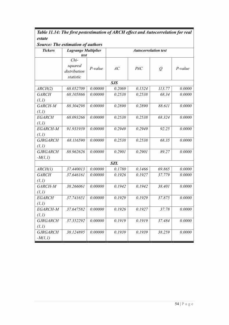
54 | P a g e


estate



test


Chi-

squared

distribution

statistic


SJS

ARCH(2) 68.052709 0.00000 0.2069 0.1524 113.77 0.0000

GARCH

(1,1)

68.105866 0.00000 0.2538 0.2538 68.34 0.0000

GARCH-M

(1,1)

88.304298 0.00000 0.2890 0.2890 88.611 0.0000

EGARCH

(1,1)

68.093266 0.00000 0.2538 0.2538 68.324 0.0000

EGARCH-M

(1,1)

91.931939 0.00000 0.2949 0.2949 92.25 0.0000

GJRGARCH

(1,1)

68.116590 0.00000 0.2538 0.2538 68.35 0.0000

GJRGARCH

-M(1,1)

88.962626 0.00000 0.2901 0.2901 89.27 0.0000

SZL

ARCH(1) 37.440013 0.00000 0.1780 0.1466 69.865 0.0000

GARCH

(1,1)

37.646161 0.00000 0.1926 0.1927 37.779 0.0000

GARCH-M

(1,1)

38.266061 0.00000 0.1942 0.1942 38.401 0.0000

EGARCH

(1,1)

37.741651 0.00000 0.1929 0.1929 37.875 0.0000

EGARCH-M

(1,1)

37.647582 0.00000 0.1926 0.1927 37.78 0.0000

GJRGARCH

(1,1)

37.352292 0.00000 0.1919 0.1919 37.484 0.0000

GJRGARCH

-M(1,1)

38.124895 0.00000 0.1939 0.1939 38.259 0.0000

55 | P a g e


insurance



test


Chi-

squared

distribution

statistic


TDH

ARCH(3) 49.082074 0.00000 0.2251 0.1740 141.12 0.0000

GARCH

(1,1)

49.250712 0.00000 0.2153 0.2153 49.419 0.0000

GARCH-M

(1,1)

49.340915 0.00000 0.2155 0.2155 49.511 0.0000

EGARCH

(1,1)

49.132172 0.00000 0.2151 0.2151 49.301 0.0000

EGARCH-M

(2,1)

49.182284 0.00000 0.1900 0.1549 87.857 0.0000

GJRGARCH

(1,1)

49.200773 0.00000 0.2152 0.2152 49.370 0.0000

GJRGARCH

-M(1,1)

49.173992 0.00000 0.2151 0.2152 49.344 0.0000

TIX

ARCH(1) 85.931701 0.00000 0.3238 0.3239 86.306 0.0000

GARCH

(1,1)

85.890301 0.00000 0.3238 0.3238 86.264 0.0000

GARCH-M

(1,1)

83.32132 0.00000 0.3189 0.3189 83.687 0.0000

EGARCH

(1,1)

86.082401 0.00000 0.3241 0.3242 86.454 0.0000

EGARCH-M

(1,2)

62.777046 0.00000 0.1941 0.1273 94.091 0.0000

GJRGARCH

(1,1)

86.053157 0.00000 0.3241 0.3241 86.427 0.0000

GJRGARCH

-M(1,1)

79.026600 0.00040 0.3106 0.3106 79.375 0.0000

56 | P a g e


estate



test


Chi-

squared

distribution

statistic


VIC

ARCH(1) 11.479916 0.00070 0.1041 0.1041 11.521 0.0007

GARCH

(1,1)

11.488838 0.00000 0.1041 0.1041 11.53 0.0007

GARCH-M

(1,1)

11.591576 0.00000 0.1046 0.1046 11.633 0.0006

EGARCH

(1,1)

11.517878 0.00000 0.1042 0.1042 11.559 0.0007

EGARCH-M

(2,1)

11.027943 0.00000 0.1548 0.1459 36.588 0.0000

GJRGARCH

(1,1)

11.509212 0.00000 0.1042 0.1042 11.55 0.0007

GJRGARCH

-M(1,1)

11.521116 0.00000 0.1042 0.1043 11.562 0.0007

VPH

ARCH(1) 6.9190805 0.00853 0.0808 0.0808 6.9423 0.0084

GARCH

(1,1)

6.9530477 0.00837 0.0810 0.0810 6.9764 0.0083

GARCH-M

(1,1)

6.7156637 0.00955 0.0796 0.0796 6.7382 0.0094

EGARCH

(1,2)

6.8608470 0.00881 0.0804 0.0805 6.8839 0.0087

EGARCH-M

(1,1)

6.8477532 0.00887 0.0804 0.0804 6.8709 0.0088

GJRGARCH

(2,1)

6.8059452 0.00908 0.0746 0.0688 12.759 0.0017

GJRGARCH

-M(2,1)

6.7661940 0.00929 0.0745 0.0687 12.697 0.0017

57 | P a g e


insurance



test


Chi-

squared

distribution

statistic


CIG

ARCH(2) 79.842295 0.00000 0.2480 0.1855 144.19 0.0000

GARCH

(1,1) 80.437250 0.00000 0.2782 0.2785 80.656 0.0000

GARCH-M

(1,1) 62.065075 0.00000 0.2444 0.2446 62.23 0.0000

EGARCH

(1,1) 81.815658 0.00000 0.2806 0.2809 82.041 0.0000

EGARCH-M

(1,1) 65.611431 0.00000 0.2513 0.2515 65.788 0.0000

GJRGARCH

(1,1) 81.297034 0.00000 0.2797 0.2800 81.52 0.0000

GJRGARCH

-M(1,1) 64.111063 0.00000 0.2484 0.2486 64.284 0.0000

DRH

ARCH(2) 72.168884 0.00000 0.2192 0.1609 122.16 0.0000

GARCH

(1,1) 72.590959 0.00000 0.2650 0.1652 72.756 0.0000

GARCH-M

(1,1) 71.653659 0.00000 0.2633 0.2635 71.813 0.0000

EGARCH

(1,1) 71.329294 0.00000 0.2627 0.2629 71.493 0.0000

EGARCH-M

(2,1) 70.525455 0.00000 0.2156 0.1585 118.88 0.0000

GJRGARCH

(1,1) 72.558921 0.00000 0.2649 0.2651 72.724 0.0000

GJRGARCH

-M(1,1) 70.921755 0.00000 0.2619 0.2621 71.08 0.0000

58 | P a g e


diversified finance group


Tickers Lagrange Multiplier test Autocorrelation test

Chi-

squared

distributio

n statistic

P-value Critical

value AC PAC Q P-value

AGR

ARCH(2) 76.475 0.0000 3.84145 0.2673 0.2699 75.881 0.000

GARCH

(1,1) 78.7112 0.0000 3.84145 0.2712 0.2737 78.131 0.000

GARCH-

M(1,1) 58.202 0.0000 3.8416 0.2332 0.2354 57.753 0.000

EGARCH

(1,1) 78.713 0.0000 3.8414 0.2712 0.2737 78.133 0.000

EGARCH

-M(1,1) 60.852 0.0000 3.8415 0.2384 0.2407 60.375 0.000

TGARCH

(1,1) 78.4419 0.0000 3.8418 0.2708 0.2733 77.860 0.000

TGARCH

-M(1,1) 57.9189 0.0000 3.8415 0.2326 0.2348 57.477 0.000

BSI

ARCH(1) 30.548 0.0000 3.8468 0.1699 0.1700 30.634 0.000

GARCH

(1,1) 29.9047 0.0000 3.8967 0.1681 0.1682 29.988 0.000

GARCH-

M(1,1) 27.546 0.0000 3.8416 0.1614 0.1614 27.624 0.000

EGARCH

(1,1) 29.527 0.0000 3.8414 0.1671 0.1671 29.610 0.000

EGARCH

-M(1,1) 29.743 0.0000 3.8264 0.1677 0.1677 29.828 0.000

TGARCH

(1,1) 30.346 0.0000 3.8414 0.1694 0.1694 30.431 0.000

TGARCH

-M(1,1) 28.346 0.0000 3.8400 0.1637 0.1637 28.426 0.000

59 | P a g e

Table 12.2: Postestimation of ARCH effect and Autocorrelation for Diversified

finance group



Chi-

squared

distributio

n statistic

P-value Critical


HCM

ARCH(3) 45.6739 0.0000 3.8414 0.2077 0.2078 45.829 0.000

GARCH

(1,1) 45.5531 0.0000 3.4812 0.2075 0.2075 45.707 0.000

GARCH-

M(1,1) 47.4866 0.0000 3.8441 0.2118 0.2119 47.647 0.000

EGARCH

(1,1) 45.4436 0.0000 3.8415 0.2072 0.2073 45.597 0.000

EGARCH

-M(1,1) 47.3538 0.0000 3.8141 0.2115 0.2116 47.513 0.000

TGARCH

(1,1) 45.464 0.0000 3.8414 0.2073 0.2073 45.617 0.000

TGARCH

-M(1,1) 47.821 0.0000 3.4811 0.2126 0.2126 47.982 0.000

OGC

ARCH(3) 22.185 0.0000 3.8411 0.1689 0.1688 15.0167 0.0002

GARCH

(1,1) 22.305 0.0000 3.8411 0.1452 0.1452 22.389 0.0000

GARCH-

M(1,1) 22.401 0.0000 3.1884 0.1455 0.1455 22.485 0.0000

EGARCH

(1,1) 22.237 0.0000 3.8415 0.1450 0.1450 22.321 0.0000

EGARCH

-M(1,2) 22.155 0.0000 3.8451 0.1447 0.1447 22.239 0.0000

TGARCH

(1,1) 22.2689 0.0000 3.8158 0.1451 0.1451 22.353 0.0000

TGARCH

-M(1,1) 22.228 0.0000 3.8451 0.1449 0.1449 22.312 0.00007

60 | P a g e

Table 12.3: The first postestimation of ARCH effect and Autocorrelation for Diversified finance

group



Chi-

squared

distributio

n statistic

P-value Critical


PTB

ARCH(4) 67.2209 0.0000 3.841 0.2546 0.2548 67.426 0.000

GARCH

(1,1)

68.1127 0.000 3.1841 0.2563 0.2565 68.317 0.000

GARCH-

M(1,1)

66.7849 0.000 3.841 0.2538 0.2540 66.985 0.000

EGARCH

(1,1)

67.233 0.000 3.841 0.2546 0.2548 67.438 0.000

EGARCH

-M(1,1)

67.044 0.000 3.815 0.2543 0.2545 67.249 0.000

TGARCH

(1,1)

67.239 0.000 8.481 0.2547 0.2548 67.444 0.000

TGARCH

-M(1,1)

66.521 0.000 3.841 0.2533 0.2535 66.724 0.000

SSI

ARCH(3) 16.472 0.000 3.854 0.1248 0.1248 16.529 0.000

GARCH

(1,1)

16.393 0.000 3.841 0.1245 0.1245 16.450 0.000

GARCH-

M(1,1)

17.952 0.000 3.811 0.1302 0.1303 18.014 0.000

EGARCH

(1,1)

16.329 0.000 3.841 0.1242 0.1242 16.386 0.000

EGARCH

-M(1,1)

17.141 0.000 3.484 0.1273 0.1273 17.200 0.000

TGARCH

(2,1)

16.090 0.000 3.841 0.1233 0.1233 16.146 0.000

TGARCH

-M(2,1)

17.771 0.000 3.841 0.1296 0.1296 17.832 0.000

61 | P a g e

Table 13.1: The first postestimation of ARCH effect and Autocorrelation for banking industry



Chi-

squared

distributio

n statistic

P-value Critical


CTG

ARCH(4) 43.40448 0.0000 3.8415 0.2017 0.2018 43.215 0.000

GARCH

(1,1) 43.41764 0.0000 3.8111 0.2017 0.2017 43.225 0.000

GARCH-

M(1,1) 41.4703 0.0000 3.8415 0.1972 0.1972 41.296 0.000

EGARCH

(1,1) 43.4235 0.0000 3.8418 0.2018 0.2018 43.230 0.000

EGARCH

-M(1,1) 41.7917 0.0000 3.8414 0.1979 0.1980 41.613 0.000

TGARCH

(1,1) 43.4345 0.0000 3.8418 0.2018 0.2018 43.237 0.000

TGARCH

-M(1,1) 41.123 0.0000 3.4481 0.1964 0.1964 40.944 0.000

EIB

ARCH(3) 145.350 0.0000 3.8415 0.3706 0.3707 145.89 0.000

GARCH

(1,1) 144.894 0.0000 3.8414 0.3701 0.3701 145.43 0.000

GARCH-

M(1,1) 139.698 0.0000 4.3841 0.3634 0.3634 140.21 0.000

EGARCH

(1,1) 146.1589 0.0000 3.8418 0.3717 0.3717 146.70 0.000

EGARCH

-M(2,1) 146.7020 0.0000 3.8611 0.3724 0.3724 147.24 0.000

TGARCH

(1,1) 145.565 0.0000 3.8411 0.3709 0.3709 146.10 0.000

TGARCH

-M(2,1) 142.269 0.0000 3.8411 0.3667 0.3667 142.79 0.000

62 | P a g e




Chi-

squared

distributio

n statistic

P-value Critical


MBB

ARCH(5) 20.7668 0.000 3.8400 0.1401 0.1401 20.838 0.000

GARCH

(1,1) 20.7939 0.000 3.8411 0.1402 0.1402 20.866 0.000

GARCH-M(1,1)

21.242 0.000 3.8411 0.1417 0.1417 21.315 0.000

EGARCH

(1,2) 20.586 0.000 3.8411 0.1395 0.1395 20.657 0.000

EGARCH

-M(1,1) 21.3508 0.000 3.8411 0.1420 0.1421 21.425 0.000

TGARCH(1,1)

20.873 0.000 3.8411 0.1404 0.1405 20.946 0.000

TGARCH

-M(1,1) 21.434 0.000 3.8144 0.1423 0.1423 21.509 0.000

STB

ARCH(2) 124.3825 0.000 3.8411 0.3425 0.3426 124.57 0.000

GARCH (1,1)

123.633 0.000 3.8411 0.3414 0.3415 123.80 0.000

GARCH-

M(1,1) 123.143

0.000 3.448 0.3408 0.3408 123.31 0.000

EGARCH

(1,1) 124.122 0.000 3.884 0.3421 0.3422 124.30 0.000

EGARCH-M(1,1)

122.3116 0.000 3.845 0.3396 0.3397 122.47 0.000

TGARCH

(1,1) 123.397 0.000 3.854 0.3411 0.3412 123.56 0.000

TGARCH-M(1,1)

6.9332 0.0084 3.840 0.1808 0.1808 6.9332 0.0085

63 | P a g e




Chi-

squared

distribution

statistic

P-value Critical


VCB

ARCH(2) 17.757 0.0000 3.844 0.1297 0.1297 17.819 0.000

GARCH

(1,1)

18.411 0.000 3.941 0.1320 0.1320 18.476 0.000

GARCH-

M(1,1)

14.907 0.000 3.841 0.1188 0.1188 14.959 0.000

EGARCH

(1,1)

18.733 0.000 3.8411 0.1332 0.1332 18.798 0.000

EGARCH

-M(1,1)

15.469 0.000 3.8414 0.1210 0.1210 15.523 0.000

TGARCH

(1,1)

18.631 0.000 3.844 0.1328 0.1329 18.696 0.000

TGARCH

-M(1,1)

15.110 0.000 3.8414 0.1196 0.1196 15.163 0.000

64 | P a g e

5.1.3. The remedial measure and model reformation

As the consequence of the first post-estimation, both symmetric and asymmetric

GARCH model could not capture the ARCH effect and autocorrelation. We refined the

model as taking the logarithm and differencing to remedy the issue. First, we also have

to test the ARCH effect on the new database (see the table 14.1 to 14.2).

The result showed that there are ARCH effect in the residual of differenced

logged return series. Hence, we will again reestimate basing on the result of the first

selection by AIC and BIC. Noting that after each new model estimation, we have to

obtain the residual to make the second postestimation to ascertain whether there are

any remaining ARCH effect or serial correlation in error terms.

And importanly, for this step we must focus on the paper’s research question

are to detect: 1) whether there are any ARCH effect in return series, 2) whether there

is asymmetry or leverage effect, meaning that volatility reacts differently to a big

increase or a big drop, 3) if the hypothesis of risk-return tradeoff is statistically

significant and 4) if Garch-family models could capture these all effect on Vietnam

financial section.

Table 14.1 : The second pre-test of ARCH effect for insurance and real estate industry.


Tickers Chi-squared statistic

test Prob Tickers

Chi-squared statistic

test Prob

BIC 111.367 0.00000 KBC 37.434 0.00000

BMI 98.620 0.00000 KDH 90.818 0.00000

BVH 107.505 0.00000 KHA 257.228 0.00000

PGI 132.112 0.00000 LHG 95.111 0.00000

ASM 58.139 0.00000 NBB 102.584 0.00000

BCI 107.574 0.00000 NTL 71.256 0.00000

CCL 407.554 0.00000 NVT 60.316 0.00000

CLG 45.709 0.00000 PDR 141.002 0.00000

D2D 94.125 0.00000 PTL 33.682 0.00000

DTA 76.112 0.00000 QCG 81.340 0.00000

DXG 42.505 0.00000 SJS 104.090 0.00000

FDC 82.938 0.00000 SZL 147.231 0.00000

FLC 41.094 0.00000 TDH 52.397 0.00000

HDC 113.886 0.00000 TIX 128.312 0.00000

HQC 52.552 0.00000 VIC 169.633 0.00000

ITC 78.253 0.00000 VPH 52.897 0.00000

CIG 33.013 0.00000 DRH 21.055 0.00000

65 | P a g e

Table 14.2: The second pre-test of ARCH effect for Diversified finance and Banks

Source: The estimation by authors

Tickers Chi-squared test statistic P-value

AGR 94.209 0.00000

BSI 35.912 0.00000

HCM 10.297 0.00130

OGC 39.027 0.00000

PTB 73.206 0.00000

SSI 128.091 0.00000

CTG 105.667 0.00000

EIB 68.864 0.00000

MBB 239.637 0.00000

STB 92.994 0.00000

VCB 158.362 0.00000

To check the appendix 2, we will display all the model result after refining

(Appendix 2: The refined models for financial industry).

ARCH model reformation result (see appendix 2.1 & 2.4): As the result after

refining, ARCH(1) was statistically significant for most of the insurance (4 tickers) and

real estate (27 tickers) while the three remainers (PDR, SJS, TIX) of real estate

followed higher order with ARCH(2) and ARCH(3). For the diversified finance and

banking industry, most were statistically captured by ARCH(1), except MBB for

ARCH(4). But the second post-test, again, showing that there was still remaining

ARCH effect and autocorrelation in residuals. Consequently, we concluded that ARCH

models were not adequate for all financial industry.

66 | P a g e

GARCH model reformation result (see apendix 2.1 & 2.4): For insurance and

real estate groups, the simplest GARCH (1,1) model was proved to be significantly

available for 22 tickers of real estate and all 4 tickers of insurance. Diversified finance

& banking also followed GARCH(1,1)

GARCH(1,2) statisfied 5 tickers of real eatate (including D2D, DXG, FDC, ITC,

PDR) and only three remainers were statistically insignificant (ASM, NVT, CIG).

Additionally, the sum of Arch term and Garch term (Φ+ θ ) for all models were less

than one showing concluding that there were no the persistent volatility.

EGARCH and GJRGARCH models reformation result (see appendix 2.2 &

2.5): The order important hypothesis of leverage effect or asymmetry that volatility

reacts differently to a big increase or a big drop was detected by EGARCH and

GJRGARCH.

The result indicated that the parameter γ was statiscally insignificant in majority

showing that both insurance & real estate stock return volatility seemed to react in the

same size on both negative or positive shocks. In particular, 27 tickers were not

available for EGARCH(1,1) and only seven remainers was weakly significant at 10%

level (as CCL, CLG, DTA, NTl, PTL, TDH, DRH). Beside, GJRGARCH (1,1) were

also not applicable for 25 tickers in majority (in constrast, BCI, CCL, CLG, DTA, LHG,

NBB, PTL, VPH, PDR).

For diversified finance and banking industry, majority was not significant with

the asymmetry parameter γ. The exception were BSI, SSI, EIB, AGR, and MBB.

Particularly, only three ticker followed asymmetric EGARCH (BSI, SSI, EIB) and

GJRGARCH( AGR, BSI, MBB).

GARCH-M model reformation result (see appendix 2.3 & 2.6): The third

hypothesis of risk-return trade-off was captured by GARCH-M, EGARCH-M and

GJRGARCH-M. The result showed that high volatilty (high risk) were not necessarily

lead to high return. As result, GARCH-M (1,1) were not available for 26 tickers (3

tickers of insurance and 23 of real estate).Additionally, EGARCH-M(1,1) was not

statistically significant for 33 tickers (4 of insurance and 29 of real estate). And 26

tickers were not available for for GJRGARCH-M(1,1). It could be concluded that there

was inefficient risk-return tradeoff for insurance and real estate on HOSE.

67 | P a g e

Otherwise, there also seemed that high volatility did not neccesarily lead to high

return in the diversified finance and banking industry (see appendix 2.6).

The second post-estimation: The post-test showed the unstatisfactory result that

both symmetric and asymmetric GARCH models could not capture the

heteroscedaticity and autocorrelation in error terms (see appendix 3.1 and 3.2). Since

the Lagrange Multiplier specified that both symmetric and asymmetric GARCH could

not capture the leverage effect, we rejected these models. In brief, we could use

GARCH-family models to describe the volatility of financial industry in HOSE.

Futhermore, we continued others same test on the four market-weighted indexes

such as Vnindex, HNXindex, VN30 index and UPCOM index. Finally, we found it

statically significant for Vnindex, HNXindex and VN30 index (see section 5.2.2).

5.2. The market-weighted indexes volatility modelling

The symmetric and asymmetric GARCH were applied to detect whether:

1/GARCH models could capture the market volatility, 2/There are any risk-return

tradeoff, 3/There are any leverage effect in market volatility, 4/ Market volatility could

be forecasted.

We also conduct the same progress as financial industry: first is the pre-test of

stationarity, heteroscedasticity and autocorrelation; second is the model estimation,

third is the post-estimation. The phase of remedial meaure to refining models will be

executed if the first post-estimation was not satisfied.

5.2.1. Pre-estimation

The Dickey-Fuller test shows that the null hypothesis of non-stationarity was

rejected. The absolute of test statistic was larger than the critical value and the p-value

was less than the significance level (1%, 5% and 10%) (see table 15.1)

The Lagrange Multiplier test of heteroscedasticity indicates that there are ARCH

effect in all four residuals while the ACF and PACF showed the autocorrelation in

residual (see table 15.2).

After pre-testing, we adapte symmetric and asymmetric GARCH to model

matket volatility as discussed on table 16.1 to table 16.3. Comparing to the post-

estimation, ARCH(2) and GARCH(1,1) could capture the heteroscedasticity in the

residual due to the result of LM test and Autocorrelation (see table 17.1 to table 17.2) .

68 | P a g e

ARCH(2) and GARCH(1) will be used to forecast the volatility of Vnindex, HNXindex

and VN30 index for the following 14 days from 11/04/2016 to 29/04/2016.

Table 15.1: The pretesting of Stationarity for Vnindex, HNXindex, VN30index,

UPCOMindex


Tickers Test statistic 1% Critical

value

5% Critical

value

10% Critical

value P-value

VNindex -30.417 -3.439 -2.860 -2.571 0.00000

HNXindex -33.373 -3.340 -2.860 -2.570 0.00000

VN30index -30.464 -3.430 -2.860 -2.570 0.00000

UPCOMindex -18.852 -3.420 -2.830 -2.570 0.00000

Table 15.2: The pretest of heteroscedasticity & autocorrelation for VNindex, HNXindex,

VN30index and UPCOMindex


ARCH effect test Autocorrelation test

Tickers Lagrange

Multiplier

test

statistic

P-value AC PAC Q statistic P-value

VNindex 15.794 0.00010 0.1222 0.1222 15.848 0.0001

HNXindex 29.166 0.00000 0.1660 0.1660 29.271 0.0000

VN30index 16.681 0.00000 0.1255 0.1255 16.738 0.0000

UPCOMindex 449.943 0.00000 0.6521 06521 451.58 0.0000

69 | P a g e

5.2.2. Model estimation of the four market-weighted indexes:

As previous applications, both symmetric and asymmetric GARCH-type models

were utilized to describe the market volatility. Phillip Hans Franses & Dick Van Dijk,

in 1996, applied GJRGARCH (1992) to capture the cross-country market-weighted

indexes such as DAX (Germany), EOE (The Netherlands), MAD (Spain), MIL (Italy)

and VEC (Sweden) covering the historical data of 9 years (Phillip & Dick, 1996).

Another paper, in 2013, by Mohd. Aminul Islam, that symmetric GARCH and

GARCH-M were employed to model the volatility of the three market-weighted

indexes including KLCI (Kuala Lumpur Composite Index), JKSE (Jakarta Stock

Exchange Composite Index) and STI (Straits Time Index). Author directly used the

simplest GARCH(1,1) and GARCH-M(1,1) spanning the period from Jan 2007 to Dec

2012. Paper was found that risk-return tradeoff was statistically significant only for

Indonesian market, except Malaysia and Singapore. (Mohd. Aminul Islam, 2013,

Middle-east journal of scientific research, ISSN:1990-9233, p.991-999).

Suliman Zakaria and Peter Winker, in 2012, applied both symmetric and

asymmetric GARCH to capture the two market-weighted indexes such as KSE

(Khartoum Stock Exchange, from Sudan) and CASE ( Cairo and Alexandria Stock

Exchange, from Egypt). In particular, GARCH(1,1), GARCH-M(1,1), EGARCH(1,1)

and TGARCH(1,1) were all displayed to cover the period of 2nd Jan 2006 to 30th Nov

2010. The positive risk premium was significantly found. (Suliman Zakaria and Peter

Winker, 2012, International journal of economics and finance,ISSN: 1916-971X,

p.161-176)

The orther older paper in 1993, published on The Journal of Finance by Glosten,

Jagannathan and Runkle, disclosed the GARCH-M to model the Center for Research

in Security Price (CRSP) value-weighted stock index during the period April 1951 to

December 1989. The negative relation between return and volatility was detected.

In our papers, ARCH and univariate GARCH models will be employed on the

volatility descriptions with the sample including the four Vietnamese market-weighted

indexes (VNindex, HNXindex, VN30 index and UPCOM index) (see table 16.1 to

16.3).

70 | P a g e

ARCH model estimation result (see table 16.1): ARCH(2) was adequately

defined as the proper model after using the information criterions, except for UPCOM

index. We will display the ARCH parameter for the lag 1 and 2 preparing for the step

of forecasting. Noting that all ARCH parameters were statistically significant and non-

zero at 1% level.

GARCH model estmation result (see table 16.1): We found that the total of

ARCH and GARCH parameter persistent volatility (Φ+ θ) for HNX and UPCOM

nearly converge to 1. It means that the past volatility would lead to the future volatility.

GARCH(1,1) was found to be statistically significant for all indexes

EGARCH and GJRGARCH model estimation result (see table 16.2): The

asymmetric parameter was significant for Vnindex and UPCOM index at 1%

significance level. The EGARCH(1,1) was 5% significant for HNXindex but

insignificant for VN30 index. And GJRGARCH(1,1) was 10% significant for VN30

but insignificant for HNXindex. In short, it might have the leverage effect on the

volatility for Vietnam stock market.

GARCH-M, EGARCH-M and GJRGARCH-M model estimation result (see

table 16.3): We found no significant risk-return tradeoff for the four market-weighted

indexes meaning that the higher volatility (higher risk) will not be necessarily

correspondent with higher return.

In brief, ARCH(2) and GARCHs with the lowest order (1,1) was available and

then, these defined models must suffer the post-testing of heteroscedasticity and

autocorrelation to define which could be used to forecast the market volatility.

5.2.3. The post estimation

As can be seen the result from table 17.1 to table 17.2, ARCH(2) and

GARCH(1,1) could capture the time-varying volatility of the market indexes such as

Vnindex, HNXindex and VN30 index but for UPCOM index.

The Lagrange Multiplier test showed the p-value exceeding the significance α

meaning that we could accept the null hypothesis of time-unvariant residual. And the

p-value of Q statistic for autocorrelation was also less then the significance α. The null

hypothesis of no serial correlation was accepted. ARCH(2) and GARCH(1,1) could be

used to forecast the market volatility.

71 | P a g e

Table 16.1: The estimation of ARCH, GARCH result of the four market-weighted indexes


Model Equation Parameter VNINDEX HNXINDEX VN30 INDEX UPCOM INDEX

ARCH

Mean μ 0.0008306** 0.0004727* 0.0006019* Invalid

Variance

Φ0 0.0000788*** 0.0000901*** 0.0000813***

Φ1 0.1494969*** 0.158548*** 0.157263***

Φ2 0.2355293*** 0.3314383*** 0.2082811***

AIC

BIC

-6569.475

-6554.58

-6323.151

-6308.256

-6563.053

-6548.155

GARCH

Mean μ 0.0006828** 0.0004694 0.0004603 0.0002833**

Variance

Φ0 0.0000116*** 0.000000*** 0.0000086*** 0.000000166***

Φ (1)0.1565037*** (1)0.1155778*** (1)0.13777195*** (1)0.1012399***

θ (1)0.7557016*** (1)0.8710014*** (1)0.7967006*** (1)0.8807393***

Φ+ θ 0.9122053 0.9865792 0.93447255 0.9819793

AIC

BIC

-6616.451

-6596.591

-6460.22

-6440.359

-6633.819

-6613.955

-7548.878

-7529.018

GARCH-M

Mean μ 0.000405 0.0003669 -0.0001149 0.0003558**

Variance

c 2.566829 0.9435362 5.557381 -3.15801

Φ0 0.0000113*** 0.00000312*** 0.0000083*** 0.000000158***

Φ (1)0.1543702*** (1)0.1159454*** (1)0.1356207*** (1)0.1081602***

θ (1)0.7606089*** (1)0.8704742*** (1)0.8010735*** (1)0.8023172***

Φ+ θ 0.914979 0.9864196 0.9366942 0.9104774

AIC

BIC

-6614.655

-6589.83

-6458.298

-6433.473

-6632.873

-6608.043

-7549.058

-7524.222

72 | P a g e

Table 16.2: EGARCH and GJRGARCH estimation result of the four market-weighted indexes



EGARCH

Mean μ 0.0004994 0.0003939 0.0005236 0.0003468***

Variance

Φ0 -1.325305*** -0.2608818*** -17.49597*** -0.0615494***

ɣ (2)-0.0708678*** (1)-0.0227351** (1)0.0024879 (1)0.0499549***

Φ (2)0.2711623*** (1)0.230143*** (1)0.0765889*** (1)0.1683549***

θ (1)0.8532738*** (1)0.9697897*** (1)-0.945692*** (1)0.9926451***

AIC

BIC

-6616.978

-6592.153 -6461.517

-6436.691

-6506.231

-6481.401

-7591.82

-7566.995

GJRGARCH

Mean μ 0.0005895* 0.0004387 0.000379 0.0003216**

Variance

Φ0 0.0000139*** 0.00000322*** 0.00000952*** 0.000000153***

Φ (1)0.2011086*** (1)0.1216902*** (1)0.1628951*** (1)0.0484485***

ɣ (1)-0.0882181*** (1)-0.0100559 (1)-0.0462696* (1)0.0912867***

θ (1)0.7331019*** (1)0.8688823*** (1)0.7860669*** (1)0.9140669***

AIC

BIC

-6618.801

-6593.975

-6458.39

-6433.564

-6633.644

-6608.814

-7565.186

-7540.36

73 | P a g e

Table 16.3: GARCH-M, EGARCH-M and GJRGARCH-M estimation result of the four market-weighted indexes



GARCH-M

Mean μ 0.000405 0.0003669 -0.0001149 0.0003558**

c 2.566829 0.9435362 5.557381 -3.15801

Variance Φ0 0.0000113*** 0.00000312*** 0.0000083*** 0.000000158***

Φ (1)0.1543702*** (1)0.1159454*** (1)0.1356207*** (1)0.1081602***

θ (1)0.7606089*** (1)0.8704742*** (1)0.8010735*** (1)0.8023172***

Φ+ θ 0.914979 0.9864196 0.9366942 0.9104774

AIC

BIC -6614.655

-6589.83

-6458.298

-6433.473

-6632.873

-6608.043

-7549.058

-7524.222

EGARCH-M

Mean μ 0.0007523 0.0004402 0.0000924 0.000339***

c -1.698545 -0.4345045 2.390025 0.4130149

Variance

Φ0 -0.8252703*** -0.2596914*** -0.5923131*** -0.0610052***

ɣ (1)-0.0404881** (1)-0.0228924** (1)-0.0240563* (1)0.0504118***

Φ (1)0.270256*** (1)0.2300183*** (1)0.2515014*** (1)0.1684329***

θ (1)0.9084383*** (1)0.9699215*** (1)0.9341488*** (1)0.992688***

AIC

BIC -6622.322

-6592.532

-6459.529

-6429.739

-6632.632

-6602.836

-7589.87

-7560.079

GJRGARCH-M

Mean μ 0.0007013 0.0003673 -0.0000449 0.0003202**

c -1.063606 0.6858798 4.183319 0.0506474

Variance

Φ0 0.0000141*** 0.00000324*** 0.00000924*** 0.000000153***

Φ (1)0.2034057*** (1)0.1213631*** (1)0.1577001*** (1)0.0483861***

ɣ (1)-0.0911446*** (1)-0.0090799 (1)-0.0398955 (1)0.0914409***

θ (1)0.7309562*** (1)0.8686612*** (1)0.7900146*** (1)0.9140806***

AIC

BIC -6616.833

-6587.043

-6456.431

-6426.64

-6632.227

-6602.431

-7563.189

-7533.398

74 | P a g e

Table 17.1: The post-estimation for Vnindex and HNXindex


Tickers

Postestimtion of

Heteroscedasticity Post estimation of autocorrelation

Chi-

squared

distibution

TR2 test

P-value Critical

value AC PAC

Q

statistic

test

P-value

VNindex

ARCH(2) 4.61924 0.103165 4.84145 0.0661 0.0661 4.6362 0.13130

GARCH(1,1) 4.73101 0.106125 4.84145 0.0661 0.0662 4.4662 0.11240

GARCH-

M(1,1)

4.77392 0.000172 3.84146 0.1155 0.1155 5.162 0.00020

EGARCH(2,1) 15.58681 0.000079 3.84146 0.1214 0.1214 15.64 0.00010

EGARCH-

M(1,1)

16.511917 0.000048 3.84146 0.1249 0.1249 16.568 0.00000

TGARCH(1,1) 15.633084 0.000076 3.84145 0.1215 0.1216 15.687 0.00000

TGARCH-

M(1,1)

16.53052 0.000048 3.841458 0.1250 0.1250 16.587 0.00000

HNXindex

ARCH(2) 0.746493 0.387588 3.84145 0.0266 0.0266 0.74894 0.38680

GARCH(1,1) 0.764690 0.084785 3.84150 0.0162 0.0166 0.79800 0.39680

GARCH-

M(1,1)

8.947501 0.000000 3.84145 0.1654 0.1654 9.05100 0.00000

EGARCH(1,1) 29.13817 0.000000 3.84158 0.1659 0.1660 29.243 0.00000

EGARCH-

M(1,1)

29.18639 0.000000 3.84581 0.1661 0.1661 29.291 0.00000

TGARCH(1,1) 29.11823 0.000000 3.84145 0.1659 0.1659 29.223 0.00000

TGARCH-

M(1,1)

28.99044 0.000000 3.84145 0.1655 0.1655 29.094 0.00000

75 | P a g e

Table 17.2: The post-estimation of VN30 index and UPCOM index


Tickers

Postestimtion of

Heteroscedasticity

Post estimation of autocorrelation

Chi-

squared distibution

TR2 test

P-value Critical

value

AC PAC Q

statistic test

P-value

VN30index

ARCH(2) 4.47718 0.343503 4.59089 0.0650 0.0650 4.4935 0.1340

GARCH(1,1) 4.71280 0.343020 4.89050 0.0650 0.0650 4.4950 0.1210

GARCH-

M(1,1)

5.68500 0.001450 3.88410 0.1217 0.1217 6.7380 0.0001

EGARCH(1,1) 16.5022 0.000048 3.80401 0.1248 0.1248 16.559 0.0000

EGARCH-

M(1,1)

16.3783 0.000052 3.84146 0.1243 0.1244 16.434 0.0000

TGARCH(1,1) 16.70144 0.000043 3.84145 0.1256 0.1256 16.759 0.0000

TGARCH-

M(1,1)

15.8006 0.000070 3.84145 0.1221 0.1222 15.855 0.0000

UPCOMindex

ARCH Invalid

GARCH(1,1) 259.24784 0.00000 3.84145 0.4946 0.4955 259.74 0.00000

GARCH-

M(1,1)

474.78442 0.00000 3.84154 0.6699 0.6699 476.54 0.00000

EGARCH(1,1) 451.06687 0.00000 3.84145 0.6529 0.6529 452.71 0.00000

EGARCH-

M(1,1)

448.48545 0.00000 3.84145 0.6510 0.6511 450.12 0.00000

TGARCH(1,1) 451.21703 0.00000 3.80140 0.6530 0.6531 452.87 0.00000

TGARCH-

M(1,1)

450.90142 0.00000 3.48158 0.6528 0.6528 452.55 0.00000

76 | P a g e

5.2.4. Volatility forecasting and error measure

We applied ARCH(2) and GARCH(1,1) to forecast the volatility of Vnindex,

HNXindex and VN30 index (see table 18.1 to table 18.6). And the 1-step ahead

forecasting will be again employed to make forecasting for the following 14 days from

08/04/2016 to 29/04/2016. The day of 08/04/2016 will be the origin time. Additionally,

we need to remember ARCH and GARCH which were used in short-term forecasting.

Otherwise, we will compare the result of 14 days forecasting and 1 day

forecasting to test the accuracy of the Vietnam stock market by the mean absolute

percenatge error (MAPE) and Theil’s inequality coefficient (TIC) (see table 19).

For Vnindex, ARCH(2) forecasting for 1 day had the lower value of MAPE and

TIC than GARCH(1,1). And, for 14 days, ARCH(2) also provide more satisfactory

result (noting that TIC is ranged from 0 to 1, the closer zero the more accurate). The

poorest was 14-days forecasting by GARCH(1,1).

For HNXindex, if we predict in 1 day, GARCH(1,1) would be more available

and the same as 14-days forecasting.

However, VN30 index was much more complicated. For 14-days prediction,

GARCH(1,1) would be the better while for 1-day, ARCH(2) could be more successful.

In brief, the ARCH and GARCH models would be more available for short-term

forecasting, especially for 1-day. However, on Vietnamese stock market, it is still not

ready for intraday trading (T+0). For 14-days ahead prediction, the result was also

accurate. In 2017, we expect that the disclipine for intraday trading would be valid and

our research would be more applicable.

6. Conclusion and further researches

We find that both symmetric and asymmetric GARCH models are not available

for Financial industry listed on HOSE. However, the application of short-term

volatility forecasting on the four Vietnamese market-weighted indexes are statistically

significant. ARCH(2) and GARCH(1,1) are found to be significant. The forecast

accuracy would be dependent on the different length of prediction for each marker

index.

The hypothesis of risk-return tradeoff is insignificantly found showing that higher

risk (higher volatility) does not neccerarily lead to higher return. And the term of

77 | P a g e

leverage effect is statistically insignificant signing by the parameter γ of EGARCH and

GJRGARCH models. Both asymmetric models could not capture the time-varying

volatility and autocorrelation due to LM test and autocorrelation function.

Importantly, the progress of model building can not be ignored the post-

estimation of heteroscedasticity and autocorrelation. Before deciding to use the

estimated model to forecast, you must ascertain that there are no remaining ARCH

effect and serial correlation in residual, if not, reject it. But we found some papers (see

the literature review) which did not execute this post-step, the result could be less

reliable and biased.

Despite our unexpected results for financial industry, as we recommended in the

introduction section that there are very few papers conducting on Vietnamese stock

market. Moreover, there is no single one investigating for a whole industry to figure

out the proper volatility models. Our current papers are conducted on a whole financial

industry listed on HOSE which include four sub-industries (insurance, real estate,

diversified finance and banks). In addition, we conduct on the four market-weighted

indexes to describe the market volatility.

Limitation and further researches

First, our limitation is the time contraint so that we can not investigate on all

industries of both Hanoi Stock Exchange and Hochiminh Stock Exchanged. If it can

be tested all industries, we will found the proper time-series models for each industry.

Moreover, some previous researches shows that others variables, for instance:

daily trading volume, daily crude oil prices, could impact the stock return volatility.

Anh the hypothesis of “Friday effect” also can be detected by ARCH and GARCH

models.

For our further researched, following the result of significant volatility modelling

for market-weighted index, as well as market risk modelling, we would carefully

consider others new variable such as crude oil, daily trading volume which can be

added to find the relationship with volatility. Moreover, we will conduct both

symmetric and asymmetric for all industries in Vietnam to detect the proper model for

each group.

78 | P a g e

Table 18.1: ARCH(2) forecasting for Vnindex from 11/04/2016 to 29/04/2016


Date Forecast variance Actual Variance Residual of var (є) Squared residual of var Residual of mean (u)

11/04/2016 0.008687932% 0.013672271% -0.004984339% 2.48436E-09 -0.000000465

12/04/2016 0.009182634% 0.000015875% 0.009166759% 8.40295E-09 0.000000878

13/04/2016 0.009273465% 0.001277096% 0.007996369% 6.39419E-09 0.000000770

14/04/2016 0.009284491% 0.000452623% 0.008831868% 7.80019E-09 0.000000851

15/04/2016 0.009288046% 0.000005095% 0.009282952% 8.61732E-09 0.000000895

19/04/2016 0.009289606% 0.042727067% -0.033437461% 1.11806E-07 -0.000003223

20/04/2016 0.009192861% 0.000098472% 0.009094389% 8.27079E-09 0.000000872

21/04/2016 0.009274842% 0.016902530% -0.007627688% 5.81816E-09 -0.000000735

22/04/2016 0.009249258% 0.080088328% -0.070839070% 5.01817E-07 -0.000006813

25/04/2016 0.009102274% 0.000393801% 0.008708473% 7.58375E-09 0.000000831

26/04/2016 0.009260330% 0.012391016% -0.003130686% 9.80119E-10 -0.000000301

27/04/2016 0.009257295% 0.006418422% 0.002838873% 8.0592E-10 0.000000273

28/04/2016 0.009270370% 0.001886920% 0.007383450% 5.45153E-09 0.000000711

29/04/2016 0.009282635% 0.011654016% -0.002371381% 5.62345E-10 -0.000000228

79 | P a g e

Table 18.2: GARCH (1,1) forecasting for Vnindex from 11/04/2016 to 29/04/2016



11/04/2016 0.0084626128% 0.013672271043% -0.000052097 0.00000000271405388 -4.792493E-07

12/04/2016 0.0088796403% 0.000015875315% 0.000088638 0.00000000785663291 8.352489E-07

13/04/2016 0.0092600549% 0.001277095871% 0.000079830 0.00000000637276350 7.681936E-07

14/04/2016 0.0096070712% 0.000452623118% 0.000091544 0.00000000838039191 8.972793E-07

15/04/2016 0.0099236212% 0.000005094595% 0.000099185 0.00000000983771707 9.880576E-07

19/04/2016 0.0102123799% 0.042727066907% -0.000325147 0.00000010572048720 -3.285815E-06

20/04/2016 0.0104757871% 0.000098471800% 0.000103773 0.00000001076886720 1.062132E-06

21/04/2016 0.0107160685% 0.016902529792% -0.000061865 0.00000000382723036 -6.404129E-07

22/04/2016 0.0109352545% 0.080088328315% -0.000691531 0.00000047821476238 -7.231459E-06

25/04/2016 0.0111351971% 0.000393801074% 0.000107414 0.00000001153775880 1.133469E-06

26/04/2016 0.0113175858% 0.012391016226% -0.000010734 0.00000000011522529 -1.141960E-07

27/04/2016 0.0114839617% 0.006418422255% 0.000050655 0.00000000256596903 5.428397E-07

28/04/2016 0.0116357308% 0.001886920380% 0.000097488 0.00000000950393039 1.051595E-06

29/04/2016 0.0117741753% 0.011654016409% 0.000001202 0.00000000000144382 1.303830E-08

80 | P a g e

Table 18.3: ARCH(2) forecasting for HNXindex from 11/04/2016 to 29/04/2016

Source: The esmation of authors


11/04/2016 0.01028759692% 0.0034683388% 0.0000681925811 0.000000004650228113 0.000000691662290

12/04/2016 0.01179448320% 0.0007880320% 0.0001100645115 0.000000012114196697 0.000001195327108

13/04/2016 0.01091960944% 0.0002470889% 0.0001067252057 0.000000011390269528 0.000001115245689

14/04/2016 0.01077824575% 0.0000846963% 0.0001069354942 0.000000011435199926 0.000001110186448

15/04/2016 0.01075566514% 0.0000106146% 0.0001074505057 0.000000011545611184 0.000001114364068

19/04/2016 0.01075222349% 0.0000106146% 0.0001074160893 0.000000011538216231 0.000001113828890

20/04/2016 0.01075166009% 0.0000106146% 0.0001074104552 0.000000011537005889 0.000001113741288

21/04/2016 0.01075156786% 0.0011870902% 0.0000956447765 0.000000009147923273 0.000000991738462

22/04/2016 0.01074750959% 0.0213698737% -0.0001062236415 0.000000011283462011 -0.000001101222576

25/04/2016 0.01067749742% 0.0000106146% 0.0001066688285 0.000000011378238980 0.000001102230091

26/04/2016 0.01073942799% 0.0000827246% 0.0001065670339 0.000000011356532724 0.000001104367083

27/04/2016 0.01074931778% 0.0081096035% 0.0000263971424 0.000000000696809128 0.000000273682713

28/04/2016 0.01072335373% 0.0002470889% 0.0001047626486 0.000000010975212535 0.000001084855227

29/04/2016 0.01074612254% 0.0034683388% 0.0000727778373 0.000000005296613608 0.000000754440580

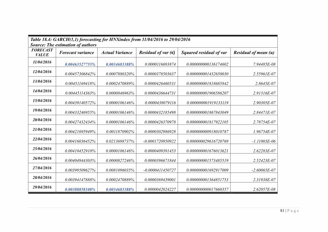
81 | P a g e

Table 18.4: GARCH(1,1) forecasting for HNXindex from 11/04/2016 to 29/04/2016

Source: The estimation of authors FORECAST

VALUE Forecast variance Actual Variance Residual of var (є) Squared residual of var Residual of mean (u)

11/04/2016 0.00463527755% 0.0034683388% 0.0000116693874 0.000000000136174602 7.94485E-08

12/04/2016 0.00457306842% 0.0007880320% 0.0000378503637 0.000000001432650030 2.55961E-07

13/04/2016 0.00451169418% 0.0002470889% 0.0000426460531 0.000000001818685842 2.8645E-07

14/04/2016 0.00445114363% 0.0000846963% 0.0000436644731 0.000000001906586207 2.91316E-07

15/04/2016 0.00439140572% 0.0000106146% 0.0000438079116 0.000000001919133119 2.90305E-07

19/04/2016 0.00433246955% 0.0000106146% 0.0000432185498 0.000000001867843049 2.84471E-07

20/04/2016 0.00427432434% 0.0000106146% 0.0000426370978 0.000000001817922105 2.78754E-07

21/04/2016 0.00421695949% 0.0011870902% 0.0000302986928 0.000000000918010787 1.96754E-07

22/04/2016 0.00416036452% 0.0213698737% -0.0001720950922 0.000000029616720769 -1.11003E-06

25/04/2016 0.00410452910% 0.0000106146% 0.0000409391453 0.000000001676013621 2.62283E-07

26/04/2016 0.00404944303% 0.0000827246% 0.0000396671844 0.000000001573485519 2.52423E-07

27/04/2016 0.00399509627% 0.0081096035% -0.0000411450727 0.000000001692917009 -2.60065E-07

28/04/2016 0.00394147888% 0.0002470889% 0.0000369439001 0.000000001364851753 2.31938E-07

29/04/2016 0.00388858108% 0.0034683388% 0.0000042024227 0.000000000017660357 2.62057E-08

82 | P a g e

Table 18.5: ARCH(2) forecasting for VN30 index from 11/04/2016 to 29/04/2016


FORECAST VALUE Forecast variance Actual Variance Residual of var (є) Squared residual of var Residual of mean (u)

11/04/2016 0.008554352261% 0.01686743431% -0.008313082052% 0.000000691073% -0.00000076887481

12/04/2016 0.009502151362% 0.00006369632% 0.009438455041% 0.000000890844% 0.00000092005096

13/04/2016 0.009643499752% 0.00285422351% 0.006789276242% 0.000000460943% 0.00000066671591

14/04/2016 0.009660452134% 0.00054712747% 0.009113324668% 0.000000830527% 0.00000089572680

15/04/2016 0.009667887980% 0.00108790953% 0.008579978446% 0.000000736160% 0.00000084362997

19/04/2016 0.009667972285% 0.02757905290% -0.017911080613% 0.000003208068% -0.00000176112218

20/04/2016 0.009613733479% 0.00000162339% 0.009612110087% 0.000000923927% 0.00000094246401

21/04/2016 0.009661514312% 0.01533764150% -0.005676127186% 0.000000322184% -0.00000055792358

22/04/2016 0.009637778232% 0.04408015413% -0.034442375896% 0.000011862773% -0.00000338128336

25/04/2016 0.009575240176% 0.00058157449% 0.008993665688% 0.000000808860% 0.00000088005857

26/04/2016 0.009654160953% 0.01318803041% -0.003533869459% 0.000000124882% -0.00000034722243

27/04/2016 0.009641010327% 0.00476261786% 0.004878392466% 0.000000237987% 0.00000047900275

28/04/2016 0.009656150929% 0.00116397308% 0.008492177847% 0.000000721171% 0.00000083448994

29/04/2016 0.009665936112% 0.00803579048% 0.001630145632% 0.000000026574% 0.00000016026857

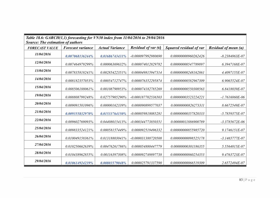
83 | P a g e

Table 18.6: GARCH(1,1) forecasting for VN30 index from 11/04/2016 to 29/04/2016


FORECAST VALUE Forecast variance Actual Variance Residual of var (є) Squared residual of var Residual of mean (u)

11/04/2016 0.007068136244% 0.01686743431% -0.000097992980690 0.00000000960262426 -8.2384863E-07

12/04/2016 0.007464979299% 0.00006369632% 0.000074012829782 0.00000000547789897 6.3947168E-07

13/04/2016 0.007835818241% 0.00285422351% 0.000049815947314 0.00000000248162861 4.4097155E-07

14/04/2016 0.008182357053% 0.00054712747% 0.000076352295874 0.00000000582967309 6.9065524E-07

15/04/2016 0.008506188061% 0.00108790953% 0.000074182785269 0.00000000550308563 6.8418039E-07

19/04/2016 0.008808799248% 0.02757905290% -0.000187702536503 0.00000003523224221 -1.7616860E-06

20/04/2016 0.009091581096% 0.00000162339% 0.000090899577037 0.00000000826273311 8.6672549E-07

21/04/2016 0.009355832970% 0.01533764150% -0.000059818085281 0.00000000357820333 -5.7859375E-07

22/04/2016 0.009602769093% 0.04408015413% -0.000344773850351 0.00000011886900789 -3.3785672E-06

25/04/2016 0.009833524121% 0.00058157449% 0.000092519496332 0.00000000855985720 9.1746151E-07

26/04/2016 0.010049158361% 0.01318803041% -0.000031388720508 0.00000000098525178 -3.1465777E-07

27/04/2016 0.010250662639% 0.00476261786% 0.000054880447779 0.00000000301186355 5.5564015E-07

28/04/2016 0.010438962855% 0.00116397308% 0.000092749897738 0.00000000860254353 9.4763723E-07

29/04/2016 0.010614924239% 0.00803579048% 0.000025791337590 0.00000000066519309 2.6572494E-07

84 | P a g e

Table 19: The forecast error measure of the three market-weigthed indexes


Tickers Model Error

measure 14 days 1 days Model

Error

measure 14 days 1 days

VNindex

ARCH(2)

MAPE 2547.077 0.366

GARCH(1,1)

MAPE 2672.769 0.381

TIC 0.661 0.095

TIC 0.621 0.105

HNXindex

MAPE 4408.69 1.966

MAPE 1748.093 0.336

TIC 0.615 0.394

TIC 0.595 0.040

VN30 index

MAPE 6122.654 0.493

MAPE 5766.099 0.581

TIC 0.457 0.193

TIC 0.464 0.287

85 | P a g e

APPENDIX 1: THE FIRST MODEL ESTIMATION FOR FINANCIAL INDUSTRY

Appendix 1.1.1: The first estimation of ARCH, GARCH result for Insurance industry (BIC,BMI,BVH,PGI)


Model Equation Parameter BIC BMI BVH PGI

ARCH

Mean μ 0.0012151 0.0018619** 0.0010167 0.0013928*

Variance Φ0 0.0005051*** 0.0004862*** 0.0005246*** 0.0006039***

Φ (1)0.3016102*** (3)0.227259*** (3)0.3291053*** (1)0.1875451***

AIC

BIC

-4725.383

-4710.488

-4838.149

-4823.259

-4647.356

-4632.461

-4406.388

-4391.653

GARCH

Mean μ 0.001454* 0.001376** 0.0007543 0.0014754*

Variance

Φ0 0.0003368*** 0.0000684*** 0.0000699*** 0.0001245***

Φ (1)0.2626804*** (1)0.1669123*** (1)0.2250166*** (1)0.1687454***

θ (1)0.2687226** (1)0.7257419*** (1)0.2250166*** (1)0.6676921***

Φ+ θ 0.531403 0.8926542 0.9092454 0.8364375

AIC

BIC

-4728.708

-4708.848

-4906

-4886.148

-4772.219

-4752.359

-4430.976

-4411.329

GARCH-M

Mean μ -0.0017362 0.0006854 -0.0000263 -0.0017011

Variance

c 4.904167 1.379233 1.394707 5.091715

Φ0 0.0003824*** 0.0000705*** 0.0000698*** (1)0.0001427***

Φ (1)0.2695667*** (1)0.1695222*** (1)0.2243438*** (1)0.1781321***

θ (1)0.1962612* (1)0.719897*** (1)0.6848445*** (1)0.6337542***

Φ+ θ 0.4658279 0.8894192 0.9091882 0.8118863

AIC

BIC

-4728.859

-4704.034

-4904.239

-4879.423

-4770.765

-4745.94

-4430.922

-4406.363

86 | P a g e

Appendix 1.1.2: The first estimation of ARCH, GARCH result for real estate industry (ASM,BCI,CCL,CLG)


Model Equation Parameter ASM BCI CCL CLG

ARCH

Mean μ 0.0007765 0.0013917* -0.0003038 -0.0006553

Variance Φ0 0.0006341*** 0.0004684*** 0.0007292*** 0.0007724***

Φ (2)0.2209264*** (3)0.1798353*** (2)0.1959518*** (3)0.2024323***

AIC

BIC

-4560.417

-4545.522

-4824.545

-4809.716

-4397.26

-4382.391

-4347.899

-4333.017

GARCH

Mean μ 0.0012123 0.000851 -0.0005192 -0.0008678

Variance

Φ0 0.0000788*** 0.000781*** 0.0000749** 0.0000633***

Φ (1)0.1165909*** (1)0.1427007*** (1)0.1394731*** (1)0.1307947***

θ (1)0.784504*** (1)0.7208277*** (1)0.7777979*** (1)0.8023041***

Φ+ θ 0.9010949 0.8635284 0.917271 0.9330988

AIC

BIC

-4595.74

-4575.88

-4868.032

-4848.26

-4454.145

-4434.319

-4427.731

-4407.89

GARCH-M

Mean μ 0.0029556 -0.0005851 -0.0008471 -0.0020002

Variance

c -2.403344 2.912207 0.4259562 1.391861

Φ0 0.000077*** 0.0000889*** 0.0000756** 0.0000656***

Φ (1)0.1159878*** (1)0.1502566*** (1)0.1404767*** (1)0.1331573***

θ (1)0.7872936*** (1)0.6941028*** (1)0.7759945 (1)0.7975698***

Φ+ θ 0.9032814 0.8443594 0.9164712 0.9307271

AIC

BIC

-4594.367

-4569.541

-4866.75

-4842.034

-4452.174

-4427.391

-4426.117

-4401.316

87 | P a g e

Appendix 1.1.3: The first estimation of ARCH, GARCH result for real estate industry (D2D,DTA, DXG, FDC)


Model Equation Parameter D2D DTA DXG FDC

ARCH

Mean μ 0.0012197 -0.0000253 0.0016323* 0.0001422

Variance Φ0 0.0004912*** 0.000878*** 0.1574551*** 0.0005934***

Φ (1)0.2470064*** (1)0.2420454*** (2)0.1574551*** (1)0.3819175***

AIC

BIC

-4048.286

-4033.909

-3748.23

-3733.663

-4586.066

-4571.16

-3657.043

-3642.745

GARCH

Mean μ 0.0013768* -0.0003496 0.0010052 0.00000

Variance

Φ0 0.005782*** 0.0000762** 0.000103 0.0001258***

Φ (1)0.251675*** (1)0.1315233*** (1)0.0770213*** (1)0.2448486***

θ (2)-0.1370761* (1)0.8041581*** (2)0.9092271*** (2)0.6203863***

Φ+ θ 0.1145989 0.9356814 0.9862484 0.8652349

AIC

BIC

-4048.321

-4029.152

-3778.355

-3758.933

-4648.754

-4628.879

-3679.347

-3660.282

GARCH-M

Mean μ -0.0019362 -0.007791*** -0.0009626 -0.002474

Variance

c 5.907659 7.162156*** 2.968513 3.326528

Φ0 0.000565*** 0.0000942** 0.0000109 0.0001272***

Φ (1)0.2484655*** (1)0.1553125*** (1)0.078973*** (1)0.2426725***

θ (2)-0.1165884 (1)0.7656376*** (2)0.9066033*** (2)0.6208653***

Φ+ θ 0.1318771 0.9209501 0.9855763 0.8635378

AIC

BIC

-4048.188

-4024.226

-3784.377

-3760.100

-4648.053

-4623.208

-3679.548

-3655.717

88 | P a g e

Appendix 1.1.4: The first estimation of ARCH, GARCH result for real estate industry (FLC, HDC, HQC, ITC)


Model Equation Parameter FLC HDC HQC ITC

ARCH

Mean μ 0.00000 0.000231 0.0009776 0.0003778

Variance Φ0 0.0010547*** 0.0005581*** 0.0006814*** 0.0005439***

Φ (3)0.1277488** (1)0.2168495 (2)0.1791151*** (4)0.1622735***

AIC

BIC

-4112.3

-4097.408

-4450.256

-4435.53

-4544.556

-4529.649

-4801.404

-4786.498

GARCH

Mean μ 0.0001693 0.0008295 0.0005249 0.0001412

Variance

Φ0 0.0001647*** 0.0000292*** 0.0000207** 0.00000

Φ (1)0.2004091*** (1)0.1533959*** (1)0.0687742*** (1)0.0897037***

θ (1)0.6636534*** (1)0.8133475*** (1)0.9054722*** (2)0.8975601***

Φ+ θ 0.8640625 0.9667434 0.9742464 0.9872638

AIC

BIC

-4204.969

-4185.112

-4517.338

-4497.703

-4592.263

-4572.387

-4909.842

-4889.967

GARCH-M

Mean μ 0.0001745 0.0002752 -0.0031784 0.0005182

Variance

c -0.0052156 1.082787 5.162641* -0.7673427

Φ0 0.0001647*** 0.0000298*** 0.0000302** 0.000000

Φ (1)0.2003907*** (1)0.1540537*** (1)0.0686485*** (1)0.089809***

θ (1)0.6636747*** (1)0.811833*** (1)0.9061838*** (2)0.8974785***

Φ+ θ 0.8640654 0.9658867 0.9748323 0.9872875

AIC

BIC

-4202.969

-4178.148

-4515.605

-4491.061

-4593.707

-4568.863

-4907.954

-4883.109

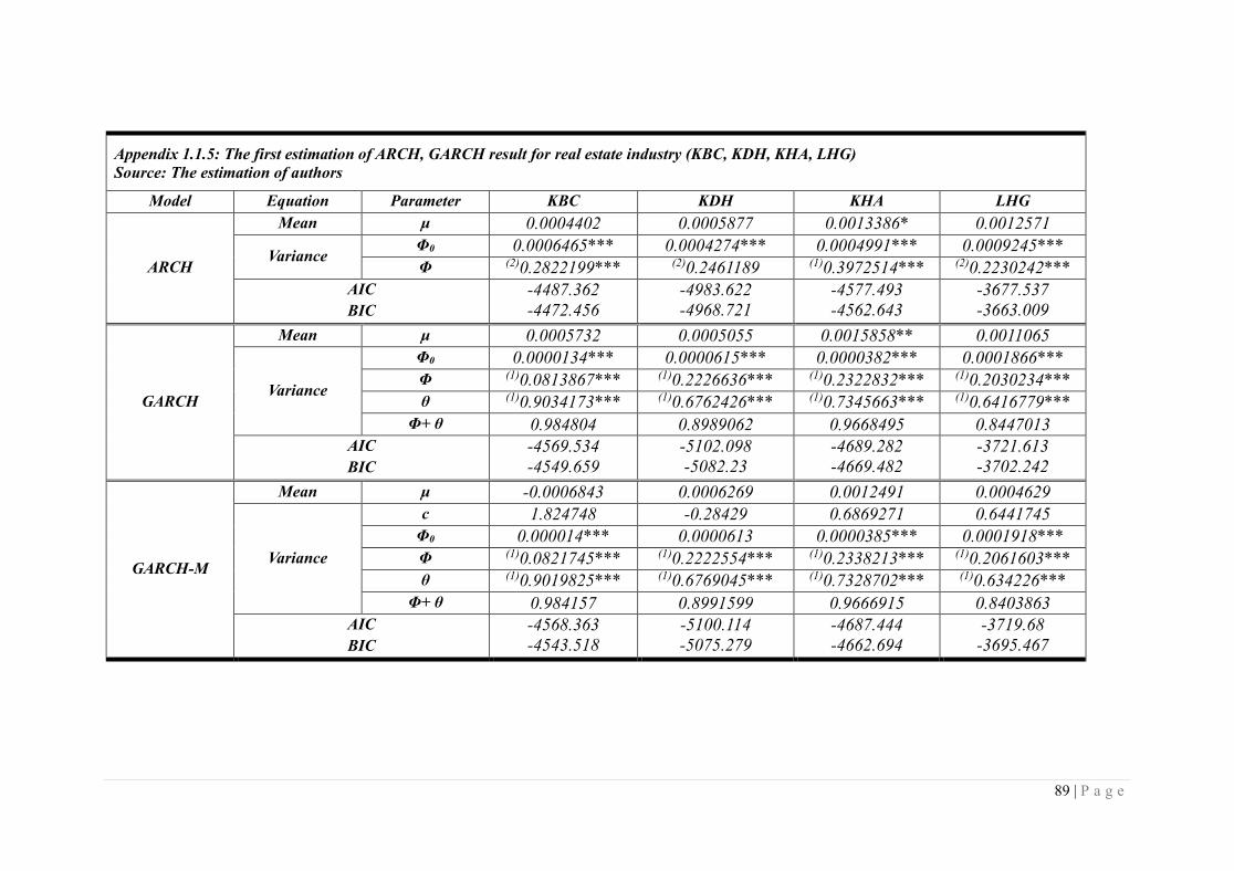
89 | P a g e

Appendix 1.1.5: The first estimation of ARCH, GARCH result for real estate industry (KBC, KDH, KHA, LHG)


Model Equation Parameter KBC KDH KHA LHG

ARCH

Mean μ 0.0004402 0.0005877 0.0013386* 0.0012571

Variance Φ0 0.0006465*** 0.0004274*** 0.0004991*** 0.0009245***

Φ (2)0.2822199*** (2)0.2461189 (1)0.3972514*** (2)0.2230242***

AIC

BIC

-4487.362

-4472.456

-4983.622

-4968.721

-4577.493

-4562.643

-3677.537

-3663.009

GARCH

Mean μ 0.0005732 0.0005055 0.0015858** 0.0011065

Variance

Φ0 0.0000134*** 0.0000615*** 0.0000382*** 0.0001866***

Φ (1)0.0813867*** (1)0.2226636*** (1)0.2322832*** (1)0.2030234***

θ (1)0.9034173*** (1)0.6762426*** (1)0.7345663*** (1)0.6416779***

Φ+ θ 0.984804 0.8989062 0.9668495 0.8447013

AIC

BIC

-4569.534

-4549.659

-5102.098

-5082.23

-4689.282

-4669.482

-3721.613

-3702.242

GARCH-M

Mean μ -0.0006843 0.0006269 0.0012491 0.0004629

Variance

c 1.824748 -0.28429 0.6869271 0.6441745

Φ0 0.000014*** 0.0000613 0.0000385*** 0.0001918***

Φ (1)0.0821745*** (1)0.2222554*** (1)0.2338213*** (1)0.2061603***

θ (1)0.9019825*** (1)0.6769045*** (1)0.7328702*** (1)0.634226***

Φ+ θ 0.984157 0.8991599 0.9666915 0.8403863

AIC

BIC

-4568.363

-4543.518

-5100.114

-5075.279

-4687.444

-4662.694

-3719.68

-3695.467

90 | P a g e

Appendix 1.1.6: The first estimation of ARCH, GARCH result for real estate industry (NBB, NTL, NVT, PDR)


Model Equation Parameter NBB NTL NVT PDR

ARCH

Mean μ -0.0002677 0.0001687 -0.0000989 -0.0000941

Variance Φ0 0.0005848*** 0.0004777*** 0.0007412*** 0.0006069***

Φ (2)0.210993*** (3)0.2176026*** (1)0.1920239*** (2)0.2924854

AIC

BIC

-4380.517

-4365.812

-4890.291

-4875.385

-4385.991

-4371.119

-3956.878

-3942.398

GARCH

Mean μ -0.001016 0.0002711 -0.0000755 0.0007913

Variance

Φ0 0.0001773 0.0000346*** 0.0001637** 0.0000306***

Φ (1)0.300393*** (1)0.1017037*** (1)0.1412199*** (1)0.1693193***

θ (1)0.4708338*** (1)0.8410354*** (1)0.680355*** (2)0.7943991***

Φ+ θ 0.600786 0.9427391 0.8215749 0.9637184

AIC

BIC

-4476.533

-4456.926

-4952.011

-4932.135

-4399.146

-4379.316

-4103.405

-4084.098

GARCH-M

Mean μ -0.0024954* -0.0003849 -0.0069549** 0.0017391

Variance

c 2.646371 1.27849 8.17186** -1.695518

Φ0 0.000182*** 0.0000337*** 0.0001895*** 0.0000297***

Φ (1)0.3025308*** (1)0.1001228*** (1)0.1518365*** (1)0.1689785***

θ (1)0.462353*** (1)0.8441368*** (1)0.6408416*** (2)0.7954904***

Φ+ θ 0.7648838 0.9442596 0.7926781 0.9644689

AIC

BIC

-4475.939

-4451.43

-4950.164

-4925.32

-4402.284

-4377.496

-4102.28

-4078.148

91 | P a g e

Appendix 1.1.7: The first estimation of ARCH, GARCH result for real estate industry (PTL,QCG,SJS,SZL)


Model Equation Parameter PTL QCG SJS SZL

ARCH

Mean μ -0.0004038 -0.0007796 0.0004399 0.0014748**

Variance Φ0 0.0011273*** 0.0004813*** 0.0006423*** 0.0004422***

Φ (2)0.1419808** (1)0.2664325*** (2)0.2385627 (2)0.1604745***

AIC

BIC

-4031.533

-4016.632

-4833.886

-4818.979

-4533.142

-4518.249

-4801.844

-4787.076

GARCH

Mean μ -0.000928 -0.0008971 -0.0000496 0.0012957*

Variance

Φ0 0.000192 0.0000433*** 0.0001798*** 0.0000727***

Φ (1)0.1271321** (1)0.142541*** (1)0.2161678*** (1)0.1415431***

θ (1)0.726913*** (1)0.7923642*** (1)0.5661054*** (1)0.722448***

Φ+ θ 0.8540451 0.9349052 0.7822732 0.8639911

AIC

BIC

-4047.165

-4027.297

-4909.088

-4889.213

-4601.403

-4581.546

-4842.361

-4822.67

GARCH-M

Mean μ -0.0199122** -0.0017186 -0.0018642 0.0022736

Variance

c 15.33852** 1.637951 2.581036 -2.195705

Φ0 0.0004815** 0.0000439*** 0.0001808*** 0.0000665***

Φ (1)0.1668372*** (1)0.1437329*** (1)0.2162178*** (1)0.135906***

θ (1)0.4609729*** (1)0.790248*** (1)0.5646792*** (1)0.7398411***

Φ+ θ 0.6278101 0.9339809 0.780897 0.8757471

AIC

BIC

-4055.896

-4031.061

-4907.544

-4882.7

-4600.493

-4575.672

-4840.696

-4816.083

92 | P a g e

Appendix 1.1.8: The first estimation of ARCH, GARCH result for real estate industry (TDH, TIX, VIC, VPH)


Model Equation Parameter TDH TIX VIC VPH

ARCH

Mean μ 0.0005452 0.0012639* 0.0003169 0.0016971*

Variance Φ0 0.0003942*** 0.0004538*** 0.0002319*** 0.000934***

Φ (3)0.2604193*** (1)0.2762135*** (1)0.2050332*** (1)0.0959264**

AIC

BIC

-5059.137

-5044.23

-3772.071

-3757.943

-5683.061

-5668.16

-4285.687

-4270.786

GARCH

Mean μ 0.0002707 0.0012074* 0.0002879 0.0016024*

Variance

Φ0 0.000016*** 0.001204*** 0.0000651*** 0.0000418**

Φ (1)0.0904971*** (1)0.2133191*** (1)0.2625991*** (1)0.0652432***

θ (1)0.8796484*** (1)0.5967056*** (1)0.540559*** (1)0.8942933***

Φ+ θ 0.9701455 0.8100247 0.8031581 0.9595365

AIC

BIC

-5134.971

-5115.096

-3805.154

-3786.317

-5745.71

-5725.843

-4316.248

-4296.38

GARCH-M

Mean μ -0.0002434 0.0018301 -0.0002186 0.000912

Variance

c 1.23978 -1.277597 2.130265 0.7221215

Φ0 0.00000159*** 0.0001202*** 0.0000653*** 0.0000423**

Φ (1)0.090308*** (1)0.2125927*** (1)0.2635736*** (1)0.0655905***

θ (1)0.8799253*** (1)0.5975271*** (1)0.5390454*** (1)0.8934536***

Φ+ θ 0.9702333 0.8101198 0.802619 0.9590441

AIC

BIC

-5133.168

-5108.324

-3803.313

-3779.766

-5744.126

-5719.291

-4314.295

-4289.46

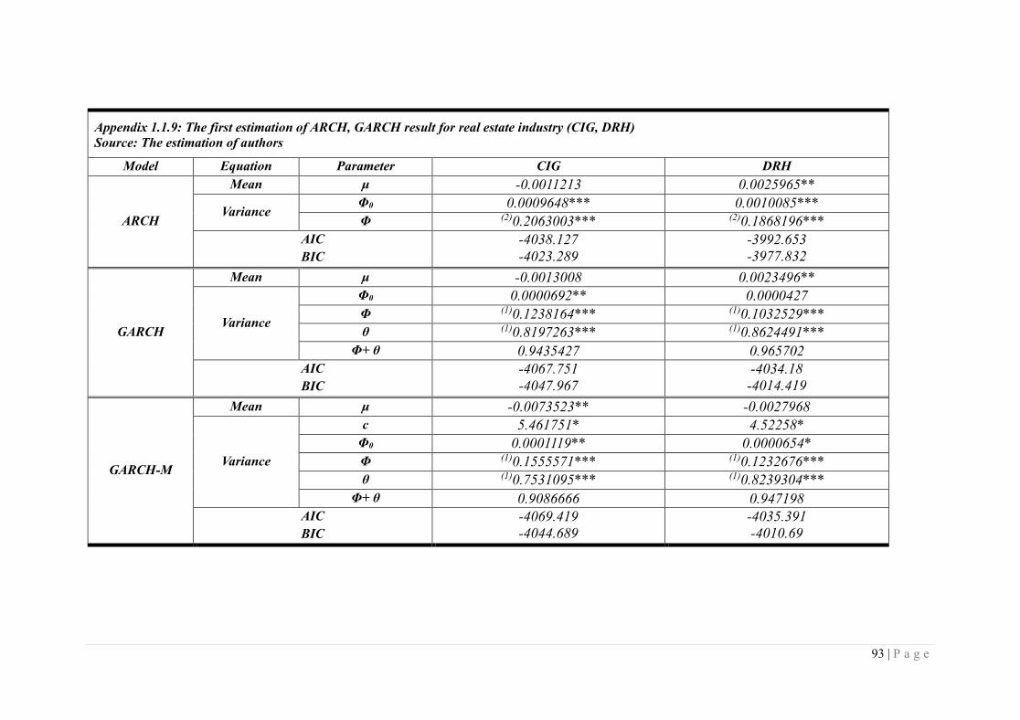
93 | P a g e

Appendix 1.1.9: The first estimation of ARCH, GARCH result for real estate industry (CIG, DRH)


Model Equation Parameter CIG DRH

ARCH

Mean μ -0.0011213 0.0025965**

Variance Φ0 0.0009648*** 0.0010085***

Φ (2)0.2063003*** (2)0.1868196***

AIC

BIC

-4038.127

-4023.289

-3992.653

-3977.832

GARCH

Mean μ -0.0013008 0.0023496**

Variance

Φ0 0.0000692** 0.0000427

Φ (1)0.1238164*** (1)0.1032529***

θ (1)0.8197263*** (1)0.8624491***

Φ+ θ 0.9435427 0.965702

AIC

BIC

-4067.751

-4047.967

-4034.18

-4014.419

GARCH-M

Mean μ -0.0073523** -0.0027968

Variance

c 5.461751* 4.52258*

Φ0 0.0001119** 0.0000654*

Φ (1)0.1555571*** (1)0.1232676***

θ (1)0.7531095*** (1)0.8239304***

Φ+ θ 0.9086666 0.947198

AIC

BIC

-4069.419

-4044.689

-4035.391

-4010.69

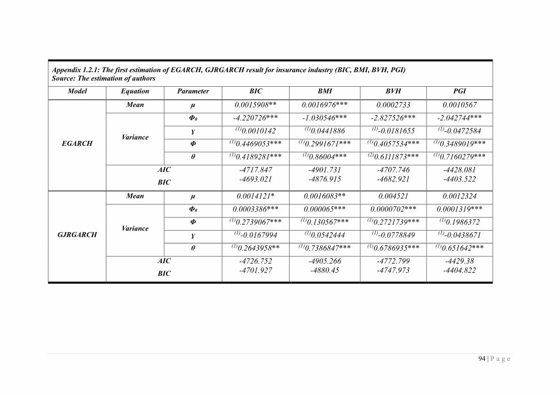
94 | P a g e

Appendix 1.2.1: The first estimation of EGARCH, GJRGARCH result for insurance industry (BIC, BMI, BVH, PGI)



EGARCH

Mean μ 0.0015908** 0.0016976*** 0.0002733 0.0010567

Variance

Φ0 -4.220726*** -1.030546*** -2.827526*** -2.042744***

ɣ (1)0.0010142 (1)0.0441886 (1)-0.0181655 (1)-0.0472584

Φ (1)0.4469053*** (1)0.2991671*** (1)0.4057534*** (1)0.3489019***

θ (1)0.4189281*** (1)0.86004*** (2)0.6111873*** (1)0.7160279***

AIC

BIC

-4717.847

-4693.021

-4901.731

-4876.915

-4707.746

-4682.921

-4428.081

-4403.522

GJRGARCH

Mean μ 0.0014121* 0.0016083** 0.004521 0.0012324

Variance

Φ0 0.0003386*** 0.000065*** 0.0000702*** 0.0001319***

Φ (1)0.2739067*** (1)0.130567*** (1)0.2721739*** (1)0.1986372

ɣ (1)-0.0167994 (1)0.0542444 (1)-0.0778849 (1)-0.0438671

θ (1)0.2643958** (1)0.7386847*** (1)0.6786935*** (1)0.651642***

AIC

BIC

-4726.752

-4701.927

-4905.266

-4880.45

-4772.799

-4747.973

-4429.38

-4404.822

95 | P a g e

Appendix 1.2.2: The first estimation of EGARCH, GJRGARCH result for real estate industry (ASM, BCI, CCL, CLG)



EGARCH

Mean μ 0.0006804 0.0010175 -0.0006033 -0.000712

Variance

Φ0 -14.13486*** -1.4891*** -0.842243*** -0.503636***

ɣ (1)0.0041659 (1)-0.0104613 (1)0.0049623 (1)0.0142337

Φ (1)0.233614 (1)0.2950172*** (1)0.2179481*** (1)0.2205861***

θ (1)-0.9835661*** (1)0.7992136 (1)0.8796866*** (1)0.9278469***

AIC

BIC

-4524.595

-4499.77

-4858.538

-4833.822

-4449.084

-4424.301

-4420.306

-4395.504

GJRGARCH

Mean μ 0.0009804 0.0007928 -0.0005231 -0.0007918

Variance

Φ0 0.0000812*** 0.0000778*** 0.000075** -0.000063***

Φ (1)0.1403604*** (1)0.1493131*** (1)0.1399889*** (1)0.1241339***

ɣ (1)-0.0463909 (1)-0.0132767 (1)-0.000688 (1)0.011065

θ (1)-0.7812909*** (1)0.7216464*** (1)0.77745*** (1)0.8040588***

AIC

BIC

-4595.633

-4570.808

-4866.133

-4841.418

-4452.145

-4427.363

-4425.854

-4401.052

96 | P a g e

Appendix 1.2.3: The first estimation of EGARCH, GJRGARCH result for real estate industry (D2D, DTA, DXG, FDC)



EGARCH

Mean μ 0.0012185 -0.0007487 0.0013447* 0.0009013

Variance

Φ0 -8.140516*** -0.754658*** -0.039982 -1.806327***

ɣ (1)-0.018332 (1)0.0015701 (1)0.0340499*** (1)0.07005197**

Φ (1)0.4589531*** (1)0.21349*** (1)0.0379159*** (1)0.3479382***

θ (2)-0.1060719 (1)0.8878919*** (2)0.9946613*** (2)0.7418786***

AIC

BIC

-4046.717

-4022.755

-3766.003

-3741.726

-4636.528

-4611.684

-3658.453

-3634.623

GJRGARCH

Mean μ 0.0010528 -0.0003028 0.0009856 0.0003802

Variance

Φ0 0.0006046*** 0.0000749** 0.0000105 0.0001198***

Φ (1)0.3084661*** (1)0.1270259*** (1)0.079706*** (1)0.1970011***

ɣ (1)-0.1037735 (1)0.006503 (1)-0.00032085 (1)0.0818932

θ (2)-0.176779** (1)0.8064716*** (2)0.9079491*** (2)0.6322336***

AIC

BIC

-4047.497

-4023.535

-3776.384

-3752.107

-4646.772

-4621.927

-3679.142

-3655.311

97 | P a g e

Appendix 1.2.4: The first estimation of EGARCH, GJRGARCH result for real estate industry (FLC, HDC, HQC, ITC)



EGARCH

Mean μ -0.0004726 0.0004625 0.0007577 0.0004986

Variance

Φ0 -1.351424*** -0.628065 -1.211564*** -0.0559688*

ɣ (1)-0.0354676 (1)-0.0313507 (1)0.0169735 (1)0.0194756

Φ (1)0.3532662*** (1)0.3057986*** (1)0.1388023*** (1)0.0619654***

θ (1)0.8001411*** (1)0.911479*** (2)0.8294954*** (1)0.9924115

AIC

BIC

-4196.104

-4171.283

-4513.987

-4489.443

-4554.295

-4529.451

-4901.654

-4876.81

GJRGARCH

Mean μ -0.0001365 0.0004435 0.0005089 0.0004239

Variance

Φ0 0.0001699*** 0.0000286*** 0.0000208** 0.00000

Φ (1)0.2383608*** (1)0.1926827*** (1)0.0699495*** (1)0.0625111***

ɣ (1)-0.0647865 (1)-0.067895 (1)-0.0018966 (1)0.0454245*

θ (1)0.6552961*** (1)0.8116357 (1)0.9052443*** (2)0.9030861***

AIC

BIC

-4204.836

-4180.016

-4517.633

-4493.089

-4590.271

-4565.427

-4911.517

-4886.673

98 | P a g e

Appendix 1.2.5: The first estimation of EGARCH, GJRGARCH result for real estate industry (KBC, KDH, KHA, LHG)



EGARCH

Mean μ 0.0007874 0.000361 0.0016647** 0.0013747

Variance

Φ0 -13.93364*** -1.332177*** -0.7023513*** -1.518776***

ɣ (1)-0.0165857 (1)-0.0109162 (1)0.0155645 (1)0.0065775

Φ (1)0.0133665 (1)0.4090365*** (1)0.4236707*** (1)0.3366024***

θ (1)-0.9837114*** (1)0.8210299 (1)0.9013492*** (1)0.7756372***

AIC

BIC

-4437.045

-4412.201

-5101.234

-5076.399

-4678.839

-4654.09

-3713.832

-3689.619

GJRGARCH

Mean μ 0.0002162 0.0003895 0.0016532** 0.0012781

Variance

Φ0 0.0000139** 0.0000604*** 0.0000381*** 0.0001846***

Φ (1)0.1090902*** (1)0.2467246*** (1)0.2256676*** (1)0.1893795***

ɣ (1)-0.0414303 (1)-0.044478 (1)0.0126184 (1)0.0298357

θ (1)0.8975362 (1)0.6781274*** (1)0.7346649*** (1)0.6426531***

AIC

BIC

-4570.541

-4545.697

-5100.737

-5075.902

-4687.332

-4662.583

-3719.85

-3695.637

99 | P a g e

Appendix 1.2.6: The first estimation of EGARCH, GJRGARCH result for real estate industry (NBB, NTL, NVT, PDR)



EGARCH

Mean μ -0.0012274* 0.0001373 0.0001092 0.0009808

Variance

Φ0 -1.6298*** -0.8582154*** -2.069233*** -0.2093846***

ɣ (1)0.0001359 (1)-0.0110615 (1)0.0025438 (1)0.0109569

Φ (1)0.4423676*** (1)0.143106*** (1)0.2452058*** (1)0.16309***

θ (1)0.7731974*** (2)0.8841741*** (1)0.7039863*** (1)0.9698734***

AIC

BIC

-4471.222

-4446.714

-4912.001

-4887.156

-4388.481

-4363.693

-4093.384

-4069.251

GJRGARCH

Mean μ -0.0010113 0.0001907 -0.0001104 0.0007271

Variance

Φ0 0.0001774*** 0.0000344*** 0.0001648** 0.0000304

Φ (1)0.2996544*** (1)0.1099166*** (1)0.1458115*** (1)0.1755249***

ɣ (1)0.0012892 (1)-0.0158069 (1)-0.0071559 (1)-0.0172604

θ (1)0.4708308*** (1)0.8413135*** (1)0.678356*** (2)0.7963229***

AIC

BIC

-4474.533

-4450.024

-4950.303

-4925.458

-4397.17

-4372.382

-4101.543

-4077.41

100 | P a g e

Appendix 1.2.7: The first estimation of EGARCH, GJRGARCH result for real estate industry (PTL, QCG, SJS, SZL)



EGARCH

Mean μ -0.0010052 -0.0010822 -0.0010083 0.0012057

Variance

Φ0 -1.578372* -0.7124512*** -1.740722*** -14.99359***

ɣ (1)0.0161098 (1)0.0151627 (1)-0.0241208 (1)-0.0102153

Φ (1)0.1826069** (1)0.2613997*** (1)0.3575154*** (1)-0.0031818

θ (1)0.7627495*** (1)0.901818*** (1)0.7547158*** (1)-0.9876418***

AIC

BIC

-4035.995

-4011.16

-4891.221

-4866.377

-4578.461

-4553.64

-4770.445

-4745.832

GJRGARCH

Mean μ -0.0008187 -0.0008937 -0.0002666 0.001546**

Variance

Φ0 0.0001969 0.0000433*** 0.0001758*** 0.0000624***

Φ (1)0.1188224* (1)0.1421335*** (1)0.2427167*** (1)0.1054877***

ɣ (1)0.0148847 (1)0.0006416 (1)-0.0538237 (1)0.0484754

θ (1)0.7236823*** (1)0.7924565*** (1)0.5726107*** (1)0.7526351***

AIC

BIC

-4045.268

-4020.433

-4907.089

-4882.244

-4600.318

-4575.497

-4841.492

-4816.879

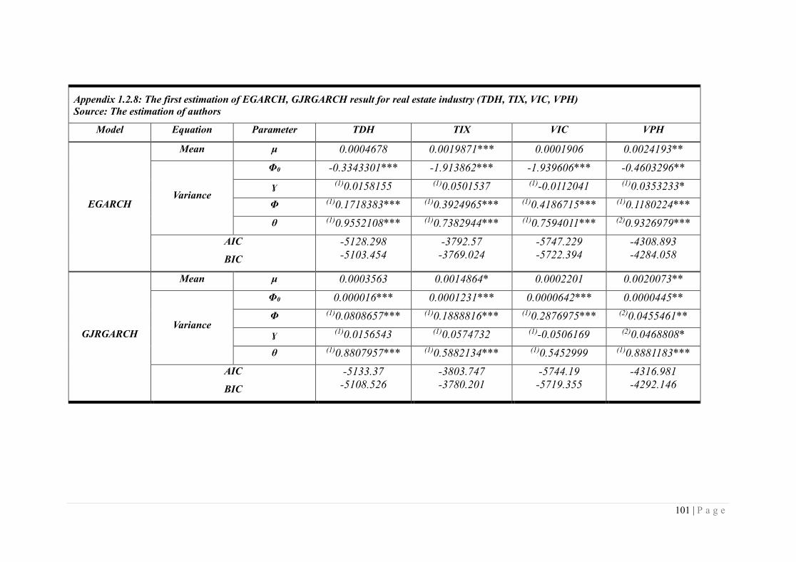
101 | P a g e

Appendix 1.2.8: The first estimation of EGARCH, GJRGARCH result for real estate industry (TDH, TIX, VIC, VPH)



EGARCH

Mean μ 0.0004678 0.0019871*** 0.0001906 0.0024193**

Variance

Φ0 -0.3343301*** -1.913862*** -1.939606*** -0.4603296**

ɣ (1)0.0158155 (1)0.0501537 (1)-0.0112041 (1)0.0353233*

Φ (1)0.1718383*** (1)0.3924965*** (1)0.4186715*** (1)0.1180224***

θ (1)0.9552108*** (1)0.7382944*** (1)0.7594011*** (2)0.9326979***

AIC

BIC

-5128.298

-5103.454

-3792.57

-3769.024

-5747.229

-5722.394

-4308.893

-4284.058

GJRGARCH

Mean μ 0.0003563 0.0014864* 0.0002201 0.0020073**

Variance

Φ0 0.000016*** 0.0001231*** 0.0000642*** 0.0000445**

Φ (1)0.0808657*** (1)0.1888816*** (1)0.2876975*** (2)0.0455461**

ɣ (1)0.0156543 (1)0.0574732 (1)-0.0506169 (2)0.0468808*

θ (1)0.8807957*** (1)0.5882134*** (1)0.5452999 (1)0.8881183***

AIC

BIC

-5133.37

-5108.526

-3803.747

-3780.201

-5744.19

-5719.355

-4316.981

-4292.146

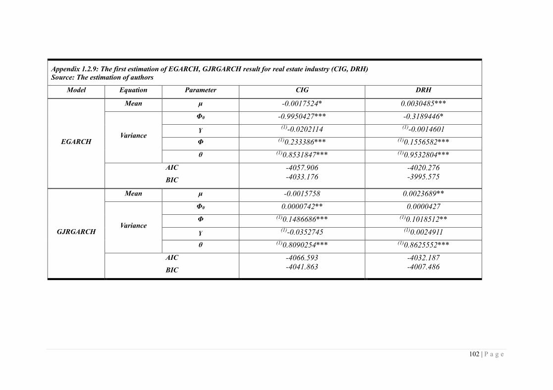
102 | P a g e

Appendix 1.2.9: The first estimation of EGARCH, GJRGARCH result for real estate industry (CIG, DRH)



EGARCH

Mean μ -0.0017524* 0.0030485***

Variance

Φ0 -0.9950427*** -0.3189446*

ɣ (1)-0.0202114 (1)-0.0014601

Φ (1)0.233386*** (1)0.1556582***

θ (1)0.8531847*** (1)0.9532804***

AIC

BIC

-4057.906

-4033.176

-4020.276

-3995.575

GJRGARCH

Mean μ -0.0015758 0.0023689**

Variance

Φ0 0.0000742** 0.0000427

Φ (1)0.1486686*** (1)0.1018512**

ɣ (1)-0.0352745 (1)0.0024911

θ (1)0.8090254*** (1)0.8625552***

AIC

BIC

-4066.593

-4041.863

-4032.187

-4007.486

103 | P a g e

Appendix 1.3.1: The first GARCH-M, EGARCH-M and GJRGARCH-M estimation result of Insurance industry (BIC,BMI,BVH,PGI)



GARCH-M

Mean μ -0.0017362 0.0006854 -0.0000263 -0.0017011

c 4.904167 1.379233 1.394707 5.091715

Variance Φ0 0.0003824*** 0.0000705*** 0.0000698*** 0.0001427***

Φ (1)0.2695667*** (1)0.1695222*** (1)0.2243438*** (1)0.1781321***

θ (1)0.1962612* (1)0.719897*** (1)0.6848445*** (1)0.6337542***

Φ+ θ 0.4658279 0.8894192 0.9091882 (1)0.8118863

AIC

BIC -4728.859

-4704.034

-4904.239

-4879.423

-4770.765

-4745.94

-4430.922

-4406.363

EGARCH-M

Mean μ -0.0010037 0.0016502 0.0006042 -0.022974***

c 4.030914 0.0947398 0.4356977 35.36682***

Variance

Φ0 -4.706503*** -1.033923*** -1.032589*** -4.378831***

ɣ (1)0.0037027 (1)0.0439631 (1)-0.0190065 (1)-0.146206***

Φ (1)0.4509177*** (1)0.299667*** (1)0.3864614*** (1)0.2218519***

θ (1)0.3523743*** (1)0.8595833*** (2)0.858509*** (1)0.3974873***

AIC

BIC -4717.037

-4687.247

-4899.732

-4869.953

-4759.919

-4730.129

-4448.139

-4418.669

GJRGARCH-M

Mean μ -0.0017177 0.0012025 0.00000 -0.010189***

c 4.846033 0.7908335 0.8276243 16.57221***

Variance

Φ0 0.0003812*** 0.0000661*** 0.0000704*** 0.0002755***

Φ (1)0.2748341*** (1)0.1338877*** (1)0.2685474*** (1)0.2890542***

ɣ (1)-0.0092063 (1)0.0520125 (1)-0.0731792 (1)-0.2101819**

θ (1)0.1976826* (1)0.7350856*** (1)0.6789682*** (1)0.4434657***

AIC

BIC -4726.872

-4697.082

-4903.343

-4873.564

-4770.984

-4741.194

-4437.023

-4407.553

104 | P a g e

Appendix 1.3.2: The first GARCH-M, EGARCH-M and GJRGARCH-M estimation result of real estate industry (ASM, BCI, CCL, CLG)



GARCH-M

Mean μ 0.0029556 -0.0005851 -0.0008471 -0.0020002

c -2.403344 2.912207 0.4259562 1.391861

Variance Φ0 0.000077*** 0.0000889*** 0.0000756** 0.0000656***

Φ (1)0.1159878*** (1)0.1502566*** (1)0.1404767*** (1)0.1331573***

θ (1)0.7872936*** (1)0.6941028*** (1)0.7759945 (1)0.7975698***

Φ+ θ 0.9032814 0.8443594 0.9164712 0.9307271

AIC

BIC

-4594.367

-4569.541

-4866.75

-4842.034

-4452.174

-4427.391

-4426.117

-4401.316

EGARCH-M

Mean μ 0.0045995* -0.001809 0.0007436 -0.0018686

c -4.70863 5.408538 -1.064308 1.557235

Variance

Φ0 -0.747668 -1.747754*** -0.812207 -0.505057***

ɣ (1)-0.0401753 (1)-0.0199556 (1)0.0079463 (1)0.016286

Φ (1)0.2000316*** (1)0.3087267*** (1)0.2083044*** (1)0.2230953***

θ (1)0.9851044*** (1)0.7647078*** (1)0.8838145*** (1)0.9276277***

AIC

BIC

-4590.299

-4560.509

-4858.51

-4828.851

-4446.746

-4417.007

-4418.601

-4388.839

GJRGARCH-M

Mean μ 0.0031153 -0.0006799 -0.0008507 -0.0019976

c -2.98187 2.972139 0.427437 1.505546

Variance

Φ0 0.0000773*** 0.0000894*** 0.0000758** 0.0000645***

Φ (1)0.1413457*** (1)0.1581425*** (1)0.1408218*** (1)0.1248668***

ɣ (1)-0.0500739 (1)-0.0153836 (1)-0.0004598 (1)0.0137637

θ (1)0.7875004*** (1)0.6931781*** (1)0.7757157*** (1)0.8001697***

AIC

BIC

-4594.587

-4564.797

-4864.873

-4835.214

-4450.174

-4420.435

-4424.3

-4394.538

105 | P a g e

Appendix 1.3.3: The first GARCH-M, EGARCH-M and GJRGARCH-M estimation result of real estate industry (D2D,DTA,DXG,FDC)



GARCH-M

Mean μ -0.0019362 -0.007791*** -0.0009626 -0.002474

c 5.907659 7.162156*** 2.968513 3.326528

Variance Φ0 0.000565*** 0.0000942** 0.0000109 0.0001272***

Φ (1)0.2484655*** (1)0.1553125*** (1)0.078973*** (1)0.2426725***

θ (2)-0.1165884 (1)0.7656376*** (2)0.9066033*** (2)0.6208653***

Φ+ θ 0.1318771 0.9209501 0.9855763 0.8635378

AIC

BIC

-4048.188

-4024.226

-3784.377

-3760.1

-4648.053

-4623.208

-3679.548

-3655.717

EGARCH-M

Mean μ -0.005335* -0.010333*** -0.0016744 0.0006678

c 10.63854** 9.920017*** 4.371225 0.3048936

Variance

Φ0 -5.882484*** -0.983566*** -0.2451726* -1.799424***

ɣ (1)-0.0863123 (1)0.0125141 (1)-0.017255 (1)0.0706425**

Φ (1)0.4254497 (1)0.2791445*** (1)0.1327441*** (1)0.3461015***

θ (1)0.200311 (1)0.8549576*** (1)0.9658899*** (2)0.7428623***

AIC

BIC

-4050.838

-4022.084

-3777.705

-3748.573

-4648.236

-4618.423

-3656.468

-3627.871

GJRGARCH-M

Mean μ -0.0062242* -0.007974*** -0.0009727 -0.0021931

c 12.19479** 7.528834*** 2.959735 3.545794

Variance

Φ0 0.0004387*** 0.00009** 0.0000112 0.0001158***

Φ (!)0.2932375*** (1)0.1404788*** (1)0.0812393*** (1)0.1916834***

ɣ (1)-0.1593562 (1)0.0268606 (1)-0.0026903 (1)0.0903109

θ (1)0.1066223 (1)0.7715743*** (2)0.9053495*** (2)0.6398109***

AIC

BIC

-4080.981

-4020.227

-3782.808

-3753.676

-4646.065

-4616.252

-3679.773

-3651.175

106 | P a g e

Appendix 1.3.4: The first GARCH-M, EGARCH-M and GJRGARCH-M estimation result of real estate industry (FLC, HDC, HQC, ITC)



GARCH-M

Mean μ 0.0001745 0.0002752 -0.0031784 0.0005182

c -0.0052156 1.082787 5.162641* -0.7673427

Variance Φ0 0.0001647*** 0.0000298*** 0.0000302** 0.000000

Φ (1)0.2003907*** (1)0.1540537*** (1)0.0686485*** (1)0.089809***

θ (1)0.6636747*** (1)0.811833*** (1)0.9061838*** (2)0.8974785***

Φ+ θ 0.8640654 0.9658867 0.9748323 0.9872875

AIC

BIC

-4202.969

-4178.148

-4515.605

-4491.061

-4593.707

-4568.863

-4907.954

-4883.109

EGARCH-M

Mean μ 0.0015188 0.0004506 -0.0029328 -0.0001106

c -1.400613 0.7883664 5.268131 1.220343

Variance

Φ0 -1.295409 -0.577265*** -0.363618*** -0.0587843*

ɣ (1)-0.0343552 (2)-0.0217126 (1)0.0091522 (1)0.0187764

Φ (1)0.3500528 (2)0.2122321*** (1)0.1375576*** (1)0.0646089***

θ (1)0.8085338 (1)0.9191544*** (1)0.9486274*** (1)0.9920103***

AIC

BIC

-4194.343

-4164.558

-4475.478

-4446.025

-4581.472

-4551.659

-4899.872

-4870.059

GJRGARCH-M

Mean μ 0.000485 -0.0002282 -0.0031826 0.0006951

c -0.6362029 1.299424 5.184509* -0.5609475

Variance

Φ0 0.0001679 0.0000299*** 0.0000202** 0.00000

Φ (1)0.239315 (1)0.1942549*** (!)0.0678945*** (1)0.0622423***

ɣ (1)-0.0681074 (1)-0.0697086 (1)0.0013123 (1)0.0452596*

θ (1)0.6579634 (1)0.8085765*** (1)0.9063592*** (2)0.9031249***

AIC

BIC

-4202.942

-4173.157

-4516.015

-4486.562

-4591.711

-4561.898

-4909.58

-4879.767

107 | P a g e

Appendix 1.3.5: The first GARCH-M, EGARCH-M and GJRGARCH-M estimation result of real estate industry (KBC, KDH, KHA, LHG)



GARCH-M

Mean μ -0.0006843 0.0006269 0.0012491 0.0004629

c 1.824748 -0.28429 0.6869271 0.6441745

Variance Φ0 0.000014*** 0.0000613 0.0000385*** 0.0001918***

Φ (1)0.0821745*** (1)0.2222554*** (1)0.2338213*** (1)0.2061603***

θ (1)0.9019825*** (1)0.6769045*** (1)0.7328702*** (1)0.634226***

Φ+ θ 0.984157 0.8991599 0.9666915 0.8403863 AIC

BIC

-4568.363

-4543.518

-5100.114

-5075.279

-4687.444

-4662.694

-3719.68

-3695.467

EGARCH-M

Mean μ -0.0001164 0.000032 0.0011673 0.0007095

c 1.127937 0.7318761 0.9419202 0.6436145

Variance

Φ0 -0.2521773 -1.381706*** -0.7220785*** -1.567801***

ɣ (1)-0.0255816 (1)-0.0099711 (1)0.010539 (1)0.0045714

Φ (1)0.1766006*** (1)0.4153358*** (1)0.4264319*** (1)0.3403483***

θ (1)0.964865*** (1)0.8141818*** (1)0.8985803*** (1)0.7684085***

AIC

BIC

-4560.189

-4530.376

-5099.306

-5069.504

-4677.13

-4647.431

-3711.888 -3682.832

GJRGARCH-M

Mean μ -0.0007222 0.0006179 0.0013208 0.000794

c 1.397824 -0.547066 0.6444609 0.474886

Variance

Φ0 0.0000147** 0.0000601*** )0.0000384*** 0.0001882***

Φ (1)0.1077393*** (1)0.2474419*** (1)0.2286719*** (1)0.1923932***

ɣ (1)-0.0391312 (1)-0.0463916 (1)0.0096101 (1)0.02828

θ (1)0.8962781*** (1)0.6791513*** (1)0.733157*** (1)0.6374527***

AIC

BIC

-4569.053

-4539.24

-5098.793

-5068.991

-46685.472

-4655.773

-3717.886 -3688.83

108 | P a g e

Appendix 1.3.6: The first GARCH-M, EGARCH-M and GJRGARCH-M estimation result of real estate industry (NBB, NTL, NVT, PDR)



GARCH-M

Mean μ -0.0024954* -0.0003849 -0.0069549** 0.0017391

c 2.646371 1.27849 8.17186** -1.695518

Variance Φ0 0.000182*** 0.0000337*** 0.0001895*** 0.0000297***

Φ (1)0.3025308*** (1)0.1001228*** (1)0.1518365*** (1)0.1689785***

θ (1)0.462353*** (1)0.8441368*** (1)0.6408416*** (2)0.7954904***

Φ+ θ 0.7648838 0.9442596 0.7926781 0.9644689

AIC

BIC

-4475.939

-4451.43

-4950.164

-4925.32

-4402.284

-4377.496

-4102.28

-4078.148

EGARCH-M

Mean μ -0.0027669* 0.0002362 -0.0093344** 0.0016959

c 2.843381 0.2690661 10.96363** -1.637121

Variance

Φ0 -1.731459*** -0.5638007*** -2.364548*** -0.2030791***

ɣ (1)-0.0038145 (1)-0.0139895 (1)-0.0018243 (1)0.0085755

Φ (1)0.4511685*** (1)0.1989109*** (1)0.2782873*** (1)0.1601386***

θ (1)0.7592885*** (1)0.9235444*** (1)0.662807*** (1)0.9708397***

AIC

BIC

-4470.458

-4441.048

-4940.017

-4910.203

-4394.322

-4364.577

-4091.703

-4062.743

GJRGARCH-M

Mean μ -0.0025025 -0.0004471 -0.0069293** 0.001691

c 2.648282 1.246575 8.107778** -1.741212

Variance

Φ0 0.0001819*** 0.0000336*** 0.0001898*** (1)0.0000294***

Φ (1)0.3034782*** (1)0.1080159*** (1)0.1550177*** (1)0.1764917***

ɣ (1)-0.0017561 (1)-0.0152779 (1)-0.0053783 (2)-0.0194226

θ (1)0.4623801 (1)0.8441467*** (1)0.6400951*** 0.7976249***

AIC

BIC

-4473.939

-4444.529

-4948.446

-4918.633

-4400.298

-4370.553

-4100.459

-4071.5

109 | P a g e

Appendix 1.3.7: The first GARCH-M, EGARCH-M and GJRGARCH-M estimation result of real estate industry (PTL, QCG, SJS, SZL)



GARCH-M

Mean μ -0.0199122** -0.0017186 -0.0018642 0.0022736

c 15.33852** 1.637951 2.581036 -2.195705

Variance Φ0 0.0004815** 0.0000439*** 0.0001808*** 0.0000665***

Φ (1)0.1668372*** (1)0.1437329*** (1)0.2162178*** (1)0.135906***

θ (1)0.4609729*** (1)0.790248*** (1)0.5646792*** (1)0.7398411***

Φ+ θ 0.6278101 0.9339809 0.780897 0.8757471 AIC

BIC

-4055.896

-4031.061

-4907.544

-4882.7

-4600.493

-4575.672

-4770.445

-4745.832

EGARCH-M

Mean μ -0.0174825 -0.0015925 -0.0041942** 0.0049629***

c 13.37501 0.9791192 4.702497* -6.458137*

Variance

Φ0 -4.10926** -0.7106541 -1.748868*** -0.6757807***

ɣ (2)0.0003908 (1)0.0148298 (1)-0.0188791 (1)0.647247**

Φ (2)0.1946034** (1)0.2639571*** (1)0.3616243*** (1)0.1920964***

θ (1)0.3819717 (1)0.9020369*** (1)0.7537044*** (1)0.9095424***

AIC

BIC

-4028.194

-3998.392

-4889.374

-4859.561

-4579.094

-4549.309

-4837.055 -4807.519

GJRGARCH-M

Mean μ -0.0204354** -0.0017141 -0.0019145 0.0034464*

c 15.67546** 1.647782 2.376795 -4.103225

Variance

Φ0 0.0004918** 0.00000438*** 0.000177*** 0.0000536***

Φ (1)0.1734357** (1)0.1425839*** (1)0.2394084*** (1)0.0873545***

ɣ (1)-0.0143426 (1)0.0017789 (1)-0.0489146 (1)0.0612614

θ (1)0.4533705*** (1)0.7905673*** (1)0.5711066*** (1)0.7798901***

AIC

BIC

-4053.982

-4024.18

-4905.546

-4875.733

-4599.257

-4569.472

-4840.667 -4811.131

110 | P a g e

Appendix 1.3.8: The first GARCH-M, EGARCH-M and GJRGARCH-M estimation result of real estate industry (TDH,TIX,VIC, VPH)



GARCH-M

Mean μ -0.0002434 0.0018301 -0.0002186 0.000912

c 1.23978 -1.277597 2.130265 0.7221215

Variance Φ0 0.00000159*** 0.0001202*** 0.0000653*** 0.0000423**

Φ (1)0.090308*** (1)0.2125927*** (1)0.2635736*** (1)0.0655905***

θ (1)0.8799253*** (1)0.5975271*** (1)0.5390454*** (1)0.8934536***

Φ+ θ 0.9702333 0.8101198 0.802619 0.9590441

AIC

BIC

-5133.168

-5108.324

-3803.313

-3779.766

-5744.126

-5719.291

-4316.248

-4296.38

EGARCH-M

Mean μ 0.0000472 0.0075643*** 0.0013832 0.0029843

c 1.086187 -10.59329*** -2.943432 -0.6659738

Variance

Φ0 -0.29543*** -2.361968*** -2.784923*** -0.4116008**

ɣ (2)0.0100013 (1)0.1010819*** (2)-0.0219859 (1)0.0249004

Φ (2)0.1419091*** (1)0.2849237*** (2)0.312162*** (1)0.1166576***

θ (1)0.9604433*** (2)0.6792141*** (1)0.6570502*** (1)0.9397754***

AIC

BIC

-5115.09

-5085.277

-3774.077

-3745.821

-5702.581

-5672.779

-4307.555

-4277.754

GJRGARCH-M

Mean μ -0.0002117 0.0031462* -0.0002237 0.0018632

c 1.38037 -3.084168 1.895636 0.1513745

Variance

Φ0 0.0000159*** 0.0001256*** 0.0000646*** 0.00000443**

Φ (1)0.0802897*** (1)0.1716946*** (1)0.2859698*** (2)0.0453431**

ɣ (1)0.0164313 (1)0.0887357 (1)-0.0458883 (1)0.0470067*

θ (1)0.8813139*** (1)0.5846318*** (1)0.5429971*** (1)0.8885545***

AIC

BIC

-5131.61

-5101.797

-3802.495

-3774.239

-5742.515

-5712.714

-4314.983

-4285.182

111 | P a g e

Appendix 1.3.9: The first GARCH-M, EGARCH-M and GJRGARCH-M estimation result of real estate industry (CIG, DRH)



GARCH-M

Mean μ -0.0073523** -0.0027968

c 5.461751* 4.52258*

Variance Φ0 0.0001119** 0.0000654*

Φ (1)0.1555571*** (1)0.1232676***

θ (1)0.7531095*** (1)0.8239304***

Φ+ θ 0.9086666 0.947198

AIC

BIC

-4069.419

-4044.689

-4035.391

-4010.69

EGARCH-M

Mean μ -0.0101444 0.001246

c 7.689594** 1.847539

Variance

Φ0 -1.687743*** -0.1080593

ɣ (1)-0.0172273 (2)0.0000721

Φ (1)0.3200321*** (2)0.1015462***

θ (1)0.7513793*** (1)0.969516***

AIC

BIC

-4059.419

-4029.743

-4007.746

-3978.105

GJRGARCH-M

Mean μ -0.0074376** -0.0031398

c 5.295579* 4.974712*

Variance

Φ0 0.0001184** 0.0000661*

Φ (1)0.1783471*** (1)0.1133077***

ɣ (1)-0.0354719 (1)0.0209845

θ (1)0.7427433*** (1)0.8228505***

AIC

BIC

-4068.075

-4038.398

-4033.779

-4004.137

112 | P a g e

Appendix 1.4.1: The first estimation of ARCH, GARCH result for diversified finance industry (AGR, BSI, HCM, OGC)


Model Equation Parameter AGR BSI HCM OGC

ARCH

Mean μ -0.000111 0.0000854 0.0017488** -0.0005445

Variance Φ0 0.00066*** 0.0007075*** 0.0004758*** 0.0007947***

Φ (2)0.1683659*** 0.1756083*** (3)0.1468585*** (3)0.2137096***

AIC

BIC

-4570.869

-4555.974

-4484.563

-4469.67

-4945.238

-4930.343

-4320.73

-4305.834

GARCH

Mean μ -0.0004931 0.0003739 0.0013097* -0.0001484

Variance

Φ0 0.0000721*** 0.0000152** 0.0000271*** 0.0001138**

Φ (1)0.1139594*** 0.0779543*** (1)0.0985406*** (1)0.1292958***

θ (1)0.7935346*** 0.9052633*** (1)0.8522953*** (1)0.7577469***

Φ+ θ 0.907494 0.9832176 0.9508359 0.8870427

AIC

BIC

-4618.633

-4598.771

-4531.977

-4512.121

-5031.151

-5011.291

-4345.15

-4325.29

GARCH-M

Mean μ -0.0052926** -0.0032654 -0.0008943 0.0004792

Variance

c 6.893955* 5.036307* 4.769825 0.3514733

Φ0 0.0000999*** 0.0000157** 0.0000254*** 0.0001152**

Φ (1)0.1331748*** 0.0791682*** (1)0.09356*** (1)0.1299927***

θ (1)0.738386*** 0.9036512*** (1)0.8601798*** (1)0.7555799***

Φ+ θ 0.8715608 0.9828194 0.9537398 0.8855726

AIC

BIC

-4620.297

-4594.472

-4534.332

-4509.512

-5031.709

-5006.884

-4343.161

-4318.335

113 | P a g e

Appendix 1.4.2: The first estimation of ARCH, GARCH result for diversified finance & banking industry (PTB, SSI,CTG,EIB)


Model Equation Parameter PTB SSI CTG EIB

ARCH

Mean μ 0.00291*** 0.0010862** 0.0002753 0.0002397

Variance Φ0 0.0005198*** 0.0003755*** 0.000267*** 0.0002146***

Φ (4)0.1498751*** (3)0.1591876*** (4)0.2638249*** (3)0.2461679***

AIC

BIC

-4746.644

-4731.812

-5185.623

-5170.728

-5464.997

-5450.101

-5716.156

-5701.261

GARCH

Mean μ 0.002599*** 0.000973* 0.0001888 0.0001326

Variance

Φ0 0.000066*** 0.00001*** 0.0000175*** 0.0000244***

Φ (1)0.1591829*** (1)0.0818183*** (1)0.1431488*** (1)0.2600158***

θ (1)0.7355038*** (1)0.8954222*** (1)0.8111561*** (1)0.6766339***

Φ+ θ 0.8946867 0.9772405 0.9543049 0.9366497

AIC

BIC

-4817.151

-4797.374

-5297.892

-5278.031

-5606.242

-5586.381

-5905.673

-5885.813

GARCH-M

Mean μ 0.002045 -0.000137 -0.0006891 0.0007112

Variance

c 1.098943 3.2754 3.735111 -3.274518

Φ0 0.0000671*** 0.0000104*** 0.0000174*** 0.0000247***

Φ (1)0.161232*** (1)0.0819829*** (1)0.1399543*** (1)0.2629305***

θ (1)0.7317845*** (1)0.8944629*** (1)0.813896 (1)0.6734343***

Φ+ θ 0.8930165 0.9764458 0.9538503 0.9363648

AIC

BIC

-4815.28

-4790.56

-5297.192

-5272.367

-5606.157

-5581.331

-5905.503

-5880.678

114 | P a g e

Appendix 1.4.3: The first estimation of ARCH, GARCH result for banking industry (MBB,STB,VCB)

Model Equation Parameter MBB STB VCB

ARCH

Mean μ 0.0004612 0.0006752 0.0014092**

Variance Φ0 0.0001623*** 0.0002373*** 0.0003339***

Φ (5)0.3058805*** (2)0.4038394*** (2)0.2046421***

AIC

BIC

-5957.041

-5942.146

-5469.485

-5454.59

-5262.275

-5247.385

GARCH

Mean μ 0.0004932 0.0001059 0.0008114

Variance

Φ0 0.00000588*** 0.0000641*** 0.0000353***

Φ (1)0.0956304*** (1)0.3702163*** (1)0.1439485***

θ (1)0.8806788*** (1)0.4911289 (1)0.7767512***

Φ+ θ 0.9763092 0.8613452 0.9206997

AIC

BIC

-6075.88

-6056.02

-5592.065

-5572.205

-5319.243

-5299.39

GARCH-M

Mean μ 0.0001966 -0.0004019 -0.0010564

Variance

c 1.910676 2.052178 5.356585

Φ0 0.00000611*** 0.000064*** 0.0000358***

Φ (1)0.0973124*** (1)0.3673887*** (1)0.1447115***

θ (1)0.8780331 (1)0.4926795*** (1)0.7745883***

Φ+ θ 0.9753455 0.8600682 0.9192998

AIC

BIC

-6074.202

-6049.376

-5590.932

-5566.107

-5319.814

-5294.998

115 | P a g e

Appendix 1.5.1: The first estimation of EGARCH, GJRGARCH result for diversified finance industry (AGR, BSI HCM, OGC)



EGARCH

Mean μ -0.0004933 0.0005401 0.0010419 -0.0003806

Variance

Φ0 -0.5687863*** -0.2747919*** -0.4237276*** -0.8794235**

ɣ (1)0.004434 (1)-0.0263186 (1)-0.0430391** (1)-0.0195718

Φ (1)0.1630075*** (1)0.1443178*** (1)0.2055995*** (1)0.2037191***

θ (1)0.9201693*** (1)0.9609309*** (1)0.9429395*** (2)0.8734906***

AIC

BIC

-4612.94

-4588.114

-4521.143

-4496.323

-5027.904

-5003.078

-4341.919

-4317.093

GJRGARCH

Mean μ -0.0004458 0.0001768 0.0010876 0.0002766

Variance

Φ0 0.0000713*** 0.0000147** 0.000031*** 0.0001107**

Φ (1)0.1085535*** (1)0.091972*** (1)0.1369143*** (1)0.139-18***

ɣ (1)0.0077763 (1)-0.0239563 (1)-0.0566569* (1)-0.0255111

θ (1)0.796032*** (1)0.9046463 (1)0.8378232*** (1)0.7638266***

AIC

BIC

-4616.68

-4591.854

-4531.188

-4506.367

-5032.642

-5007.817

-4343.636

-4318.811

116 | P a g e

Appendix 1.5.2: The first estimation of EGARCH, GJRGARCH result for diversified finance & banking industry (PTB,SSI,CTG,EIB)



EGARCH

Mean μ 0.0029059*** 0.0008844 0.0001435 0.0004378

Variance

Φ0 -1.022281*** -8.314959*** -0.633799*** -1.271764***

ɣ (1)0.0690085** (1)-0.0358378 (1)-0.0232037 (1)0.0296323

Φ (1)0.2768122*** (1)0.2340607*** (1)0.2961479*** (1)0.459711***

θ (1)0.8621054*** (1)0.1265632*** (1)0.918554 (!)0.8434876***

AIC

BIC

-4816.548

-4791.828

-5151.492

-5190.667

-5606.891

-5582.066

-5902.69

-5877.865

GJRGARCH

Mean μ 0.002904*** 0.0005661 -0.00000692 0.0002913

Variance

Φ0 0.000062*** 0.0000178*** 0.0000173*** 0.0000246***

Φ (1)0.1096161*** (2)0.1753607*** (1)0.1774418*** (1)0.2246885***

ɣ (1)0.0689573 (2)-0.1121334*** (1)-0.0579427* (1)0.0656746

θ (1)0.7530411*** (1)0.847686*** (1)0.8100742*** (1)0.6762649***

AIC

BIC

-4817.488

-4792.767

-5305.008

-5280.182

-5606.928

-5582.103

-5905.18

-5880.355

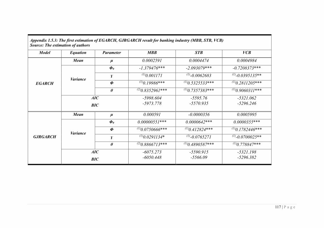
117 | P a g e

Appendix 1.5.3: The first estimation of EGARCH, GJRGARCH result for banking industry (MBB, STB, VCB)



EGARCH

Mean μ 0.0002591 0.0004474 0.0004984

Variance

Φ0 -1.379476*** -2.093079*** -0.7208373***

ɣ (1)0.001171 (1)-0.0062683 (1)-0.0395135**

Φ (1)0.19986*** (1)0.5325533*** (1)0.2811205***

θ (2)0.8352961*** (1)0.7357383*** (1)0.9060311***

AIC

BIC

-5998.604

-5973.778

-5595.76

-5570.935

-5321.062

-5296.246

GJRGARCH

Mean μ 0.000591 -0.0000356 0.0005995

Variance

Φ0 0.00000551*** 0.0000642*** 0.0000355***

Φ (1)0.0750666*** (1)0.412824*** (1)0.1782446***

ɣ (1)0.0291134* (1)-0.0765271 (1)-0.0700025**

θ (2)0.8866713*** (1)0.4890587*** (1)0.778847***

AIC

BIC

-6075.273

-6050.448

-5590.915

-5566.09

-5321.198

-5296.382

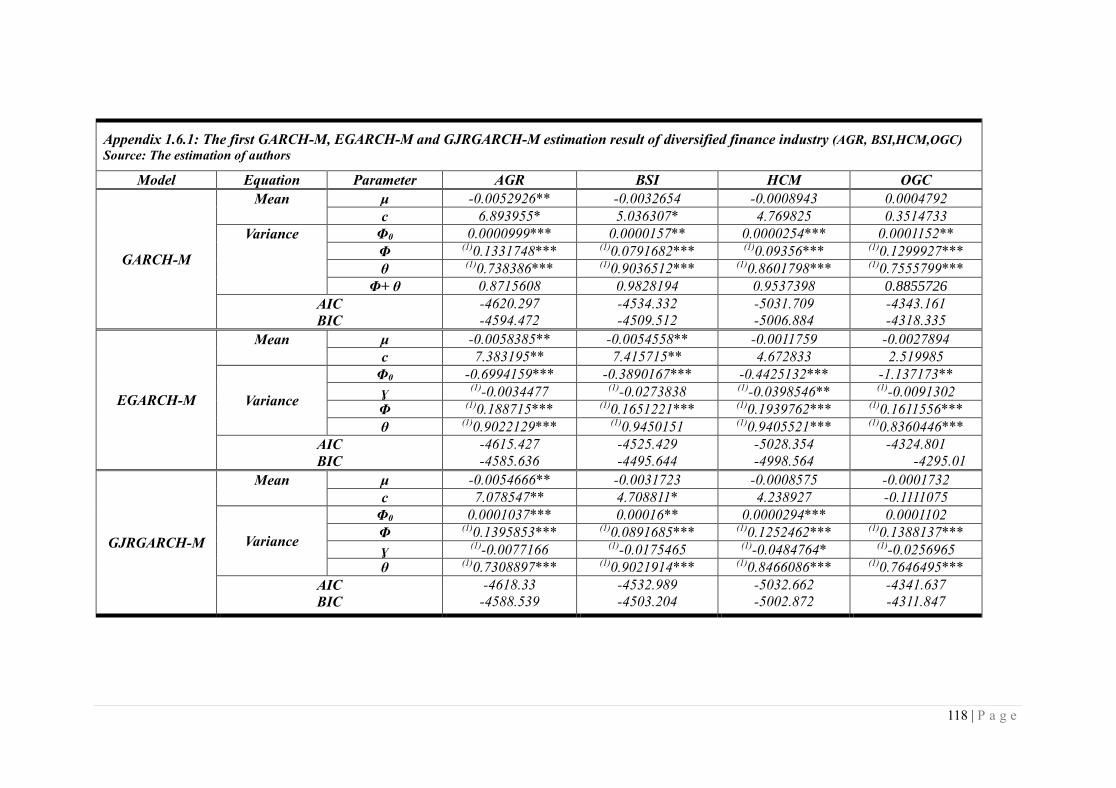
118 | P a g e

Appendix 1.6.1: The first GARCH-M, EGARCH-M and GJRGARCH-M estimation result of diversified finance industry (AGR, BSI,HCM,OGC)



GARCH-M

Mean μ -0.0052926** -0.0032654 -0.0008943 0.0004792

c 6.893955* 5.036307* 4.769825 0.3514733

Variance Φ0 0.0000999*** 0.0000157** 0.0000254*** 0.0001152**

Φ (1)0.1331748*** (1)0.0791682*** (1)0.09356*** (1)0.1299927***

θ (1)0.738386*** (1)0.9036512*** (1)0.8601798*** (1)0.7555799***

Φ+ θ 0.8715608 0.9828194 0.9537398 0.8855726

AIC

BIC

-4620.297

-4594.472

-4534.332

-4509.512

-5031.709

-5006.884

-4343.161

-4318.335

EGARCH-M

Mean μ -0.0058385** -0.0054558** -0.0011759 -0.0027894

c 7.383195** 7.415715** 4.672833 2.519985

Variance

Φ0 -0.6994159*** -0.3890167*** -0.4425132*** -1.137173**

ɣ (1)-0.0034477 (1)-0.0273838 (1)-0.0398546** (1)-0.0091302

Φ (1)0.188715*** (1)0.1651221*** (1)0.1939762*** (1)0.1611556***

θ (1)0.9022129*** (1)0.9450151 (1)0.9405521*** (1)0.8360446***

AIC

BIC

-4615.427

-4585.636

-4525.429

-4495.644

-5028.354

-4998.564

-4324.801

-4295.01

GJRGARCH-M

Mean μ -0.0054666** -0.0031723 -0.0008575 -0.0001732

c 7.078547** 4.708811* 4.238927 -0.1111075

Variance

Φ0 0.0001037*** 0.00016** 0.0000294*** 0.0001102

Φ (1)0.1395853*** (1)0.0891685*** (1)0.1252462*** (1)0.1388137***

ɣ (1)-0.0077166 (1)-0.0175465 (1)-0.0484764* (1)-0.0256965

θ (1)0.7308897*** (1)0.9021914*** (1)0.8466086*** (1)0.7646495***

AIC

BIC

-4618.33

-4588.539

-4532.989

-4503.204

-5032.662

-5002.872

-4341.637

-4311.847

119 | P a g e

Appendix 1.6.2: The first GARCH-M, EGARCH-M and GJRGARCH-M estimation result of diversified finance industry (PTB,SSI,CTG,EIB)



GARCH-M

Mean μ 0.002045 -0.000137 -0.0006891 0.0007112

c 1.098943 3.2754 3.735111 -3.274518

Variance Φ0 0.0000671*** 0.0000104*** 0.0000174*** 0.0000247***

Φ (1)0.161232*** (1)0.0819829*** (1)0.1399543*** (1)0.2629305***

θ (1)0.7317845*** (1)0.8944629*** (1)0.813896 (1)0.6734343***

Φ+ θ 0.8930165 0.9764458 0.9538503 0.9363648

AIC

BIC

-4815.28

-4790.56

-5297.192

-5272.367

-5606.157

-5581.331

-5905.503

-5880.678

EGARCH-M

Mean μ 0.0027947 -0.0016448 -0.0005873 0.001048

c 0.2017199 6.096835 2.992627 -3.293021

Variance

Φ0 -1.028206*** -8.1931*** -0.6293272*** -1.281305***

ɣ (1)0.0685543** (2)-0.0926284*** (1)-0.0239051 (2)0.0301542

Φ (1)0.2784201*** (2)0.3182633*** (1)0.2880074*** (2)0.4667429***

θ (1)0.861304*** (1)0.9669229*** (1)0.9192948*** (1)0.842136***

AIC

BIC

-4814.554

-4784.889

-5234.364

-5204.574

-5605.989

-5576.199

-5902.000

-5872.209

GJRGARCH-M

Mean μ 0.0026389 -0.0004204 -0.0008372 0.0007774

c 0.5218947 2.97574 3.569292 -2.887789

Variance

Φ0 0.0000623*** 0.0000197*** 0.0000175*** 0.0000251***

Φ (1)0.1111412*** (2)0.1734436*** (1)0.1713125*** (1)0.2320056***

ɣ (1)0.0684054 (2)-0.1080565*** (1)-0.0539245* (1)0.0558991

θ (1)0.7515739*** (1)0.8412615*** (1)0.8114549*** (1)0.6723546***

AIC

BIC

-4815.518

-4785.853

-5304.218

-5274.428

-5606.659

-5576.868

-5904.541

-5874.751

120 | P a g e

Appendix 1.6.3: The first GARCH-M, EGARCH-M and GJRGARCH-M estimation result of diversified finance industry (MBB,STB,VCB)



GARCH-M

Mean μ 0.0001966 -0.0004019 -0.0010564

c 1.910676 2.052178 5.356585

Variance Φ0 0.00000611*** 0.000064*** 0.0000358***

Φ (1)0.0973124*** (1)0.3673887*** (1)0.1447115***

θ (1)0.8780331 (1)0.4926795*** (1)0.7745883***

Φ+ θ 0.9756434 0.8600682 0.9192998

AIC

BIC

-6074.202

-6049.376

-5590.932

-5566.107

-5319.814

-5294.998

EGARCH-M

Mean μ 0.0004907 -0.0009435 -0.0010647

c 1.576462 2.755625 4.850873

Variance

Φ0 -0.3077001*** -2.097527*** -0.7691061***

ɣ (1)0.0326939*** (1)-0.019806 (1)-0.0372002**

Φ (1)0.1645997*** (1)0.53300789*** (1)0.280836***

θ (1)0.9623133*** (1)0.7350636*** (1)0.8999841***

AIC

BIC

-6074.92

-6045.13

-5594.352

-5564.561

-5321.159

-5291.38

GJRGARCH-M

Mean μ 0.0002744 -0.0004879 -0.0009004

c 2.069974 1.874209 4.367298

Variance

Φ0 0.00000567*** 0.0000644*** 0.0000368***

Φ (1)0.0763949*** (1)0.4054831*** (1)0.1749661***

ɣ (1)0.0301956* (1)-0.068684 (1)-0.062136*

θ (1)0.8843889*** (1)0.4897458*** (1)0.7738035***

AIC

BIC

-6073.658

-6043.868

-5589.616

-5559.826

-5320.892

-5291.113

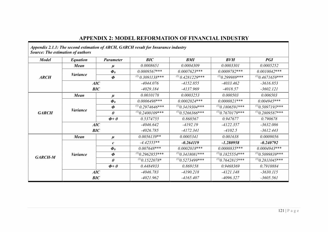
121 | P a g e

APPENDIX 2: MODEL REFORMATION OF FINANCIAL INDUSTRY

Appendix 2.1.1: The second estimation of ARCH, GARCH result for Insurance industry



ARCH

Mean μ 0.0008651 0.0004309 0.0003301 0.0005252

Variance Φ0 0.0009567*** 0.0007623*** 0.0009782*** 0.0010042***

Φ (1) 0.3091138*** (1) 0.4281229*** (1)0.299989*** (1)0.4671659***

AIC

BIC

-4044.076

-4029.184

-4152.855

-4137.969

-4033.462

-4018.57

-3616.853

-3602.121

GARCH

Mean μ 0.0010178 0.0003253 0.000503 0.006503

Variance

Φ0 0.0006498*** 0.0002024*** 0.0000821*** 0.004945***

Φ (1) 0.2974646*** (1)0.3419304*** (1)0.1806591*** (1)0.5097193***

θ (1)0.2400109*** (1)0.5266366*** (1)0.7670179*** (1)0.2809587***

Φ+ θ 0.5374755 0.868567 0.947677 0.790678

AIC

BIC

-4046.642

-4026.785

-4192.19

-4172.341

-4122.357

-4102.5

-3632.086

-3612.443

GARCH-M

Mean μ 0.0056139** 0.0005341 0.001638 0.0009056

Variance

c -4.42555** -0.264119 -1.280958 -0.240792

Φ0 0.007648*** 0.0002018*** 0.0000835*** 0.0004943***

Φ (1)0.2962855*** (1)0.3418081*** (1)0.1825554*** (1)0.5099839***

θ (1)0.1522078* (1)0.5273499*** (1)0.7642815*** (1)0.2811045***

Φ+ θ 0.4484933 0.869158 0.9468369 0.7910884

AIC

BIC

-4046.783

-4021.962

-4190.218

-4165.407

-4121.148

-4096.327

-3630.115

-3605.561

122 | P a g e

Appendix 2.1.2: The second estimation of ARCH, GARCH result for Real estate industry (ASM, BCI, CCL, CLG)



ARCH

Mean μ 0.0001235 0.0002435 -0.0034955 0.0005014

Variance Φ0 0.0011046*** 0.0006993*** 0.0145856*** 0.0012369***

Φ (1)0.2705078*** (1)0.2980862*** (8)0.3917231*** (1)0.2836892***

AIC

BIC

-3924.115

-3909.223

-4201.358

-4186.532

-1067.361

-1052.491

-3776.57

-3761.691

GARCH

Mean μ 0.0001758 0.0003588 -0.0034538 0.0005792

Variance

Φ0 0.009512*** 0.0003217*** 0.0006257*** 0.0009421***

Φ (1)0.2765983*** (1)0.4358426*** (1)0.1678058*** (1)0.2927737***

θ (1)0.0995661 (1)0.3268628*** (1)0.7988975*** (1)0.1691231**

Φ+ θ 0.3761644 0.7627054 0.9667033 0.4618968

AIC

BIC

-3922.975

-3903.118

-4231.687

-4211.918

-1361.987

-1342.161

-3777.909

-3758.072

GARCH-M

Mean μ 0.001287 -0.000389 0.0031514 -0.0033488

Variance

c -0.9337243 1.057999 -0.5681131** 2.964165

Φ0 0.0009522*** 0.0003222*** 0.0005797*** 0.0009733***

Φ (1)0.2757821*** (1)0.4372055*** (1)0.1580366*** (1)0.2995183***

θ (1)0.09955105 (1)0.3249791*** (1)0.8106078*** (1)0.1436544*

Φ+ θ 0.37533315 0.7621846 0.9686444 0.4431727

AIC

BIC

-3921.094

-3896.274

-4230.005

-4205.294

-1365.079

-1340.297

-3777.308

-3752.511

123 | P a g e

Appendix 2.1.3: The second estimation of ARCH, GARCH result for Real estate industry (CIG, DRH, D2D, DTA)


Model Equation Parameter CIG DRH D2D DTA

ARCH

Mean μ 0.0005251 0.0001827 -0.0004088 0.0005334

Variance Φ0 0.0018467*** 0.0018974*** 0.0007563*** 0.0015831***

Φ (1)0.1865114*** (1)0.1205865*** (1)0.6303801*** (1)0.2522021***

AIC

BIC

-3394.932

-3380.097

-3412.948

-3398.13

-3334.094

-3319.721

-3191.904

-3177.341

GARCH

Mean μ 0.000397 0.0001721 -0.00376 0.0006537

Variance

Φ0 0.0023327*** 0.0000473 0.0008333*** 0.0001875***

Φ (1)0.1803495*** (1)0.0417963*** (1)0.6188071*** (1)0.170288***

θ (1)-0.1211004 (1)0.9365244*** (2)-0.0392127* (1)0.7482746***

Φ+ θ 0.0592491 0.9783207 0.5795944 0.9185626

AIC

BIC

-3393.505

-3373.725

-3427.13

-3407.373

-3333.486

-3314.321

-3229.894

-3210.477

GARCH-M

Mean μ 0.0087696 0.0007355 0.002473* -0.0011648

Variance

c -4.188755 -0.2840489 -2.990088*** 1.181841

Φ0 0.0020922*** 0.0000478 0.0007975*** 0.0001992***

Φ (1)0.1831553*** (1)0.0420076*** (1)0.6948812*** (1)0.1775047***

θ (1)-0.1075343 (1)0.936106*** (2)-0.0393457** (1)0.7360581***

Φ+ θ 0.075621 0.9781136 0.6555355 0.9135628

AIC

BIC

-3392.468

-3367.743

-3425.141

-3400.445

-3334.756

-3310.8

-3228.445

-3204.173

124 | P a g e

Appendix 2.1.4: The second estimation of ARCH, GARCH result for Real estate industry (DXG, FDC, FLC, HDC)


Model Equation Parameter DXG FDC FLC HDC

ARCH

Mean μ -0.0000886 0.0007488 0.0005082 0.000332

Variance Φ0 0.0012044*** 0.001248*** 0.0018091*** 0.0008406***

Φ (1)0.1682383*** (1)0.3709691*** (1)0.1866957*** (1)0.5581147***

AIC

BIC

-3948.842

-3933.939

-3039.918

-3025.623

-3483.578

-3468.688

-3714.989

-3700.265

GARCH

Mean μ -0.0000366 0.0008448 0.0006235 0.0003797

Variance

Φ0 0.0008204*** 0.0006944*** 0.0006669*** 0.0003989***

Φ (1)0.1623744*** (1)0.3387675*** (1)0.1927107*** (1)0.5964244***

θ (2)0.2722341** (2)0.3132681*** (1)0.512729*** (1)0.2671909***

Φ+ θ 0.4346085 0.6520356 0.7054397 0.8636153

AIC

BIC

-3947.353

-3927.481

-3049.501

-3030.441

-3500.171

-3480.318

-3739.674

-3720.043

GARCH-M

Mean μ 0.0080545* -0.0043348* 0.0063429 0.0007516

Variance

c -6.401894* 4.103771*** -3.2126 -0.4143108

Φ0 0.0007726*** 0.0008198*** 0.0007109*** 0.0004007***

Φ (1)0.167047*** (1)0.4404123*** (1)0.197778*** (1)0.5970009***

θ (2)0.3005872*** (2)0.1755034*** (1)0.487589*** (1)0.2658322***

Φ+ θ 0.4676342 0.6159157 0.685367 0.8628331

AIC

BIC

-3948.271

-3923.432

-3052.834

-3029.008

-3500.193

-3475.377

-3737.789

-3713.25

125 | P a g e

Appendix 2.1.5: The second estimation of ARCH, GARCH result for Real estate industry (HQC, ITC, KBC, KDH)


Model Equation Parameter HQC ITC KBC KDH

ARCH

Mean μ -0.0003792 -0.000439 -0.0001516 0.0002285

Variance Φ0 0.0011865*** 0.0009392*** 0.0012371*** 0.0005626***

Φ (1)0.2564203*** (1)0.2696204*** (1)0.2395848*** (1)0.5130585***

AIC

BIC

-3874.674

-3859.77

-4110.346

-4095.443

-3850.911

-3836.008

-4448.141

-4433.243

GARCH

Mean μ -0.000192 0.0003083 0.0002411 0.0006037

Variance

Φ0 0.000113 0.0000216* 0.0000153* 0.0001116***

Φ (1)0.1289079*** (1)0.0880195*** (1)0.0617994*** (1)0.5096309***

θ (1)0.8027713*** (1)0.894834*** (1)0.9289411*** (1)0.4829281***

Φ+ θ 0.9316792 0.9828535 0.9907405 0.992559

AIC

BIC

-3889.672

-3869.801

-4129.874

-4110.002

-3902.393

-3882.521

-4528.292

-4508.428

GARCH-M

Mean μ -0.0012216 0.0003157 0.0010719 0.0013241

Variance

c 0.8232315 -0.0082393 -0.6678018 -1.474537

Φ0 0.0001149*** 0.0000216* 0.0000155* 0.0001112***

Φ (1)0.1299297*** (1)0.0880238*** (1)0.0623033*** (1)0.5118747***

θ (1)0.8005694*** (1)0.8948342*** (1)0.9283786*** (1)0.4820214***

Φ+ θ 0.9304991 0.982858 0.9906819 0.9938961

AIC

BIC

-3887.831

-3862.992

-4127.874

-4103.035

-3900.543

-3875.703

-4528.216

-4503.386

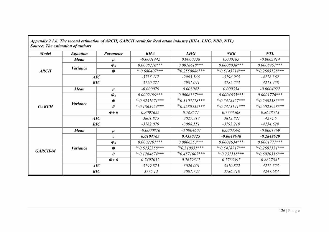
126 | P a g e

Appendix 2.1.6: The second estimation of ARCH, GARCH result for Real estate industry (KHA, LHG, NBB, NTL)


Model Equation Parameter KHA LHG NBB NTL

ARCH

Mean μ -0.0001442 0.0000338 0.000185 -0.0003914

Variance Φ0 0.0008216*** 0.0018618*** 0.0008038*** 0.0008451***

Φ (1)0.680407*** (1)0.2550086*** (1)0.5145714*** (1)0.2695128***

AIC

BIC

-3735.117

-3720.271

-2995.566

-2981.041

-3796.955

-3782.253

-4228.362

-4213.458

GARCH

Mean μ -0.000079 0.003042 0.000354 -0.0004022

Variance

Φ0 0.0002199*** 0.0006337*** 0.0004635*** 0.0001776***

Φ (1)0.6231671*** (1)0.3105178*** (1)0.5418427*** (1)0.2602585***

θ (1)0.1865954*** (1)0.4580532*** (1)0.2315141*** (1)0.6025928***

Φ+ θ 0.8097625 0.768571 0.7733568 0.8628513

AIC

BIC

-3801.875

-3782.079

-3027.917

-3008.551

-3812.821

-3793.219

-4274.5

-4254.629

GARCH-M

Mean μ -0.0000876 -0.0004607 0.0003596 -0.0001769

Variance

c 0.0104765 0.4350425 -0.0049648 -0.2848629

Φ0 0.0002201*** 0.0006353*** 0.0004634*** 0.0001777***

Φ (1)0.6232358*** (1)0.310851*** (1)0.5418717*** (1)0.2607531***

θ (1)0.1264674*** (1)0.4571007*** (1)0.231518*** (1)0.6020316***

Φ+ θ 0.7497032 0.7679517 0.7733897 0.8627847

AIC

BIC

-3799.875

-3775.13

-3026.001

-3001.793

-3810.822

-3786.318

-4272.523

-4247.684

127 | P a g e

Appendix 2.1.7: The second estimation of ARCH, GARCH result for Real estate industry (NVT, PDR, PTL, QCG)


Model Equation Parameter NVT PDR PTL QCG

ARCH

Mean μ 0.0002182 0.0003259 0.0001027 0.0002815

Variance Φ0 0.0013204*** 0.0014844*** 0.002236*** 0.000931***

Φ (1)0.260384*** (3)0.1612982*** (1)0.1661265*** (1)0.2492604***

AIC

BIC

-3710.23

-3695.36

-3244.614

-3230.137

-3283.447

-3268.549

-4145.407

-4130.503

GARCH

Mean μ 0.0002231 0.0003492 0.000143 0.0004575

Variance

Φ0 0.0014988*** 0.0000385*** 0.0013238*** 0.000156

Φ (1)0.2581755*** (1)0.1610689*** (1)0.1739184*** (1)0.242905***

θ (1)-0.100679 (2)0.8252515*** (1)0.3350983** (1)0.6460704***

Φ+ θ 0.1574965 0.9863204 0.5090167 0.8889754

AIC

BIC

-3708.692

-3688.865

-3445.516

-3426.215

-3285.652

-3265.788

-4207.597

-4187.726

GARCH-M

Mean μ -0.0033114 -0.0013422 -0.0071341 0.0014771

Variance

c 2.436554 1.856465* 3.203728 -1.209351

Φ0 0.0014818*** 0.0000528*** 0.0013857*** 0.0001576***

Φ (1)0.2611339*** (1)0.1907613*** (1)0.1814805*** (1)0.243922***

θ (1)-0.0938773 (2)0.7894415*** (1)0.3046869* (1)0.6436682***

Φ+ θ 0.1672566 0.9802028 0.4861674 0.8875902

AIC

BIC

-3707.456

-3682.673

-3445.546

-3421.418

-3284.711

-3259.881

-4206.073

-4181.234

128 | P a g e

Appendix 2.1.8: The second estimation of ARCH, GARCH result for Real estate industry (SJS, SZL, TDH, TIX)


Model Equation Parameter SJS SZL TDH TIX

ARCH

Mean μ -0.0000957 0.0006486 -0.0001354 0.0000401

Variance Φ0 0.0013207*** 0.0006384*** 0.0006783*** 0.0011971***

Φ (2)0.1144931*** (1)0.4982187*** (1)0.2928465*** (2)0.2525724***

AIC

BIC

-3889.141

-3874.251

-4093.74

-4078.976

-4437.857

-4422.953

-2996.578

-2982.453

GARCH

Mean μ 0.00000 0.0007393 -0.0001294 -0.0004193

Variance

Φ0 0.0003575*** 0.0003481*** 0.000171*** 0.000307***

Φ (1)0.2321901*** (1)0.4977461*** (1)0.2782135*** (1)0.604426***

θ (1)0.5307788*** (1)0.2655668*** (1)0.5599834*** (1)0.3042761***

Φ+ θ 0.7629689 0.7633129 0.8381969 0.9087021

AIC

BIC

-3979.264

-3959.411

-4108.675

-4088.89

-4479.711

-4459.839

-3163.313

-3144.481

GARCH-M

Mean μ 0.0001589 0.0017909 0.0004361 -0.0004747

Variance

c -0.1387707 -1.487689 -0.8673751 0.0725188

Φ0 0.0003577*** 0.0003465*** 0.0001708*** 0.0003063***

Φ (1)0.2323681*** (1)0.4998846*** (1)0.280076*** (1)0.6039921***

θ (1)0.5304928*** (1)0.2669076*** (1)0.5586441*** (1)0.3051143***

Φ+ θ 0.7628609 0.7667922 0.8387201 0.9091064

AIC

BIC

-3977.269

-3952.453

-4107.443

-4082.835

-4477.872

-4453.033

-3161.317

-3137.777

129 | P a g e

Appendix 2.1.9: The second estimation of ARCH, GARCH result for Real estate industry (VIC, VPH)


Model Equation Parameter VIC VPH

ARCH

Mean μ -0.0000319 0.0004687

Variance Φ0 0.000278*** 0.0012909***

Φ (1)0.6131687*** (1)0.3954135***

AIC

BIC

-5104.434

-5089.536

-3635.958

-3621.06

GARCH

Mean μ 0.0001049 0.0005509

Variance

Φ0 0.0001285*** 0.0010249***

Φ (1)0.6351288*** (1)0.3912581***

θ (1)0.2668865*** (1)0.1353816

Φ+ θ 0.9020153 0.5266397

AIC

BIC

-5160.366

-5140.502

-3636.622

-3616.758

GARCH-M

Mean μ 0.00087 0.0015084

Variance

c -2.64421** -0.6521796

Φ0 0.0001325*** 0.0010289***

Φ (1)0.6528509*** (1)0.3927944***

θ (1)0.247894*** (1)0.1326156

Φ+ θ 0.9007449 0.52541

AIC

BIC

-5161.976

-5137.145

-3634.76

-3609.93

130 | P a g e

Appendix 2.2.1: The second estimation of EGARCH, GJRGARCH result for insurance industry



EGARCH

Mean μ 0.0006175 0.00000 0.0011894 -

Variance

Φ0 -4.580041*** -1.905124*** -0.604943*** -

ɣ (1)-0.0235744 (1)-0.049853 (1)0.0161932 -

Φ (1)0.5867126*** (1)0.5945895*** (1)0.333982*** -

θ (1)0.3105212*** (1)0.7179371*** (1)0.9078453 -

AIC

BIC

-4201.097

-4176.286

-4101.42

-4076.60

GJRGARCH

Mean μ 0.0006562 -0.0006787 0.0008177 -0.0002821

Variance

Φ0 0.0006453*** 0.0002174*** 0.0000834*** 0.0004945***

Φ (1)0.331638*** (1)0.427514*** (1)0.1640919*** (1)0.5967167***

ɣ (1)-0.059044 (1)-0.1612476 (1)0.0345103 (1)-0.1651107

θ (1)0.2404273 (1)0.5124618*** (1)0.7654521*** (1)0.2804085***

AIC

BIC

-4044.925

-4020.105

-4192.847

-4168.035

-4120.618

-4095.797

-3631.462

-3606.908

131 | P a g e

Appendix 2.2.2: The second estimation of EGARCH, GJRGARCH result for Real estate industry (ASM, BCI, CCL, CLG)



EGARCH

Mean μ 0.0001974 -0.0003799 0.0023691 -0.003068**

Variance

Φ0 -4.915575*** -3.263678*** -0.0814598*** -4.032488***

ɣ (1)-0.0107972 (1)-0.0652603 (1)0.0824069*** (1)-0.2015604***

Φ (1)0.5181561*** (1)0.7217179*** (1)0.1520852*** (1)0.4893679***

θ (1)0.2485739** (1)0.5252604*** (1)0.9779843*** (1)0.372014***

AIC

BIC

-3929.826

-3905.005

-4239.515

-4214.804

-1355.06

-1330.277

-3795.569

-3770.772

GJRGARCH

Mean μ 0.0000434 -0.0008125 0.0004298 -0.0030211**

Variance

Φ0 0.000949*** 0.0003227 0.0003697*** 0.0009302***

Φ (1)0.2861281*** (1)0.5628792*** (1)0.0626837*** (1)0.6207723***

ɣ (1)-0.0191284 (1)-0.2402931* (1)0.1210646*** (1)-0.5198646***

θ (1)0.1010569 (1)0.3248911*** (1)0.8592443*** (1)0.1601475**

AIC

BIC

-3921.003

-3896.182

-4233.553

-4208.842

-1373.099

-1348.316

-3794.601

-3769.804

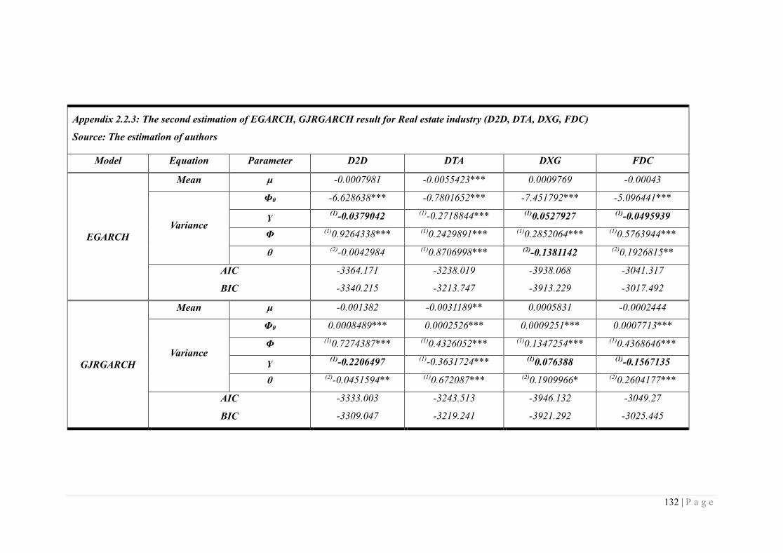
132 | P a g e

Appendix 2.2.3: The second estimation of EGARCH, GJRGARCH result for Real estate industry (D2D, DTA, DXG, FDC)



EGARCH

Mean μ -0.0007981 -0.0055423*** 0.0009769 -0.00043

Variance

Φ0 -6.628638*** -0.7801652*** -7.451792*** -5.096441***

ɣ (1)-0.0379042 (1)-0.2718844*** (1)0.0527927 (1)-0.0495939

Φ (1)0.9264338*** (1)0.2429891*** (1)0.2852064*** (1)0.5763944***

θ (2)-0.0042984 (1)0.8706998*** (2)-0.1381142 (2)0.1926815**

AIC

BIC

-3364.171

-3340.215

-3238.019

-3213.747

-3938.068

-3913.229

-3041.317

-3017.492

GJRGARCH

Mean μ -0.001382 -0.0031189** 0.0005831 -0.0002444

Variance

Φ0 0.0008489*** 0.0002526*** 0.0009251*** 0.0007713***

Φ (1)0.7274387*** (1)0.4326052*** (1)0.1347254*** (1)0.4368646***

ɣ (1)-0.2206497 (1)-0.3631724*** (1)0.076388 (1)-0.1567135

θ (2)-0.0451594** (1)0.672087*** (2)0.1909966* (2)0.2604177***

AIC

BIC

-3333.003

-3309.047

-3243.513

-3219.241

-3946.132

-3921.292

-3049.27

-3025.445

133 | P a g e

Appendix 2.2.4: The second estimation of EGARCH, GJRGARCH result for Real estate industry (CIG, DRH, FLC, HDC)


Model Equation Parameter CIG DRH FLC HDC

EGARCH

Mean μ -0.0045509** -0.0050957*** -0.0013003 -

Variance

Φ0 -0.2957082** -0.1041935** -0.0384914 -

ɣ (1)-0.2057231*** (1)-0.2310821*** (1)-0.0627743 -

Φ (1)0.0833791*** (1)0.0081527 (1)0.0350011*** -

θ (1)0.9493448*** (1)0.9810284*** (1)0.9934343*** -

AIC

BIC

-3397.337

-3372.612

-3426.248

-3401.552

-3471.15

-3446.334

-

GJRGARCH

Mean μ 0.0003176 -0.0007275 0.000367 -0.0002203

Variance

Φ0 0.0023301*** 0.0000686* 0.0006596*** 0.0004064***

Φ (1)0.1842143*** (1)0.0760628** (1)0.2040994*** (1)0.664869***

ɣ (1)-0.0074438 (1)-0.0510894 (1)-0.0232113 (1)-0.1291508

θ (1)-0.2100546 (1)0.9197381*** (1)0.5164431*** (1)0.2609058***

AIC

BIC

-3391.514

-3366.789

-3426.026

-3401.33

-3498.243

-3473.427

-3738.419

-3713.88

134 | P a g e

Appendix 2.2.5: The second estimation of EGARCH, GJRGARCH result for Real estate industry (HQC, ITC, KBC, KDH)



EGARCH

Mean μ - 0.0007901 0.0004732 -

Variance

Φ0 - -1.291135*** -0.0956651** -

ɣ - (1)0.0653325 (1)0.0066716 -

Φ - (1)0.3545849*** (1)0.1261717*** -

θ - (1)0.8068254*** (1)0.9850211*** -

AIC

BIC

- -4129.103

-4104.263

-3892.044

-3867.204

-

GJRGARCH

Mean μ -0.0002355 0.0004325 0.0004757 0.0003641

Variance

Φ0 0.0001128*** 0.0001303*** 0.0000149* 0.0001111***

Φ (1)0.1304994*** (1)0.1224412*** (1)0.0517806* (1)0.5402533***

ɣ (1)-0.0040055 (1)0.0690364 (1)0.017661 (1)-0.0629509

θ (1)0.8032816*** (1)0.7461879*** (1)0.9303515*** (1)0.4840869***

AIC

BIC

-3887.677

-3862.837

-4129.1

-4104.26

-3900.544

-3875.704

-4526.609

-4501.779

135 | P a g e

Appendix 2.2.6: The second estimation of EGARCH, GJRGARCH result for Real estate industry (KHA, LHG, NBB, NTL)



EGARCH

Mean μ -0.0001073 -0.0016067 -0.0006343 0.000798

Variance

Φ0 -2.274492*** -1.981385*** -3.345465*** -1.584232***

ɣ (1)-0.0208436 (1)-0.0933121 (1)-0.0834558 (1)0.0849292*

Φ (1)1.054438*** (1)0.5373352*** (1)0.8442849*** (1)0.4728359***

θ (1)0.646711*** (1)0.6710311*** (1)0.4938118*** (1)0.7672554***

AIC

BIC

-3837.298

-3812.554

-3030.02

-3005.811

-3838.993

-3814.489

-4270.767

-4245.927

GJRGARCH

Mean μ -0.0005705 -0.0019203 -0.0012296 0.0006367

Variance

Φ0 0.0002205*** 0.0006259*** 0.0004807*** 0.0001906***

Φ (1)0.6769625*** (1)0.4394785*** (1)0.7285231*** (1)0.2043826***

ɣ (1)-0.1113357 (1)-0.2349513* (1)-0.3427278** (1)0.1469299

θ (1)0.3877783*** (1)0.4596487*** (1)0.2167365*** (1)0.5797936***

AIC

BIC

-3800.545

-3775.8

-3030.351

-3006.143

-3816.064

-3791.56

-4275.217

-4250.378

136 | P a g e

Appendix 2.2.7: The second estimation of EGARCH, GJRGARCH result for Real estate industry (NVT, PDR, PTL, QCG)



EGARCH

Mean μ 0.00000 - -0.002831 0.0005742

Variance

Φ0 -6.021772*** - -2.777991*** -1.492534***

ɣ (1)-0.0458952 - (1)-0.1258076** (1)0.006217

Φ (1)0.4917382*** - (1)0.2734941*** (1)0.4720621***

θ (1)0.0540693 - (1)0.5305162*** (1)0.7774977***

AIC

BIC

-3715.165

-3690.383

- -3286.103

-3261.273

-4198.02

-4173.181

GJRGARCH

Mean μ -0.0008267 -0.0006166 -0.0027773 0.0003483

Variance

Φ0 0.0013996*** 0.0000348*** 0.0012741*** 0.0001552***

Φ (1)0.3349116*** (1)0.200168*** (1)0.294541*** (1)0.2501023***

ɣ (1)-0.131437 (1)-0.095558** (1)-0.2227048* (1)-0.0144518

θ (1)-0.0493126 (2)0.8379197*** (1)0.3561695** (1)0.646808

AIC

BIC

-3708.124

-3683.341

-3448.857

-3424.73

-3288.591

-3263.76

-4205.626

-4180.787

137 | P a g e

Appendix 2.2.8: The second estimation of EGARCH, GJRGARCH result for Real estate industry (SJS, SZL, TDH, TIX)



EGARCH

Mean μ -0.0001723 0.0007889 0.00000 0.0005351

Variance

Φ0 -1.754088*** -3.281193*** -13.63766*** -2.654032***

ɣ (1)-0.0238472 (1)-0.0109103 (1)-0.0085862*** (1)0.0547971

Φ (1)0.412548*** (1)0.8265518*** (1)0.0775799*** (1)0.8855204***

θ (1)0.7310553*** (1)0.5223762*** (1)-0.9689181*** (1)0.5963567***

AIC

BIC

-3960.861

-3936.046

-4124.176

-4099.568

-4387.57

-4362.73

-3173.617

-3150.077

GJRGARCH

Mean μ -0.0003074 0.0006245 0.000736 -0.000011

Variance

Φ0 0.0003547*** 0.0003501*** 0.0001728*** 0.0003073***

Φ (1)0.2479145*** (1)0.5103946*** (1)0.2185644*** (1)0.5593264***

ɣ (1)-0.0354022 (1)-0.0251439 (1)0.1421161 (1)0.0920285

θ (1)0.534427*** (1)0.2635745*** (1)0.5519487*** (1)0.3038483***

AIC

BIC

-3977.452

-3952.636

-4106.605

-4081.996

-4480.039

-4455.20

-3161.629

-3138.089

138 | P a g e

Appendix 2.2.9: The second estimation of ARCH, GARCH result for Real estate industry (VIC, VPH)



EGARCH

Mean μ 0.0010815** 0.00000

Variance

Φ0 -3.044214*** -3.95744***

ɣ (1)0.0606685 (1)-0.0684264

Φ (1)0.9291191*** (1)0.6122124***

θ (1)0.5997453*** (1)0.3682677***

AIC

BIC

-5176.125

-5151.295

-3651.871

-3627.04

GJRGARCH

Mean μ 0.0005481 -0.001731

Variance

Φ0 0.0001298*** 0.0009796***

Φ (1)0.5616156*** (1)0.5573626***

ɣ (1)0.1780333 (1)-0.3172778**

θ (1)0.2582997*** (1)0.1631913*

AIC

BIC

-5159.739

-5134.909

-3639.992

-3615.162

139 | P a g e

Appendix 2.3.1: The second GARCH-M, EGARCH-M and GJRGARCH-M estimation result of Insurance industry (BIC,BMI,BVH,PGI)



GARCH-M

Mean μ 0.0056139** 0.0005341 0.001638 0.0009056

c -4.42555** -0.264119 -1.280958 -0.240792

Variance Φ0 0.007648*** 0.0002018*** 0.0000835*** 0.0004943***

Φ (1)0.2962855*** (1)0.3418081*** (1)0.1825554*** (1)0.5099839***

θ (1)0.1522078* (1)0.5273499*** (1)0.7642815*** (1)0.2811045***

Φ+ θ 0.4484933 0.869158 0.9468369 0.7910884

AIC

BIC

-4046.783

-4021.962

-4190.218

-4165.407

-4121.148

-4096.327

-3630.115

-3605.561

EGARCH-M

Mean μ - - - -

c - - - -

Variance

Φ0 - - - -

ɣ - - - -

Φ - - - -

θ - - - -

AIC

BIC

- - - -

GJRGARCH-M

Mean μ - -0.3186666*** 0.0036117** -0.3696628*

c - 3.490657** -2.486102* 3.278391*

Variance

Φ0 - 0.009284*** 0.0000962*** 0.0013108***

Φ - (1)0.0277784** (1)0.1363282*** (1)0.0348095*

ɣ - (1)-0.0580404*** (1)0.0992992 (1)-0.0785061*

θ - (1)-0.015249 (1)0.7503352*** (1)-0.1563106***

AIC

BIC

- -4382.079

-4352.305

-4120.644

-4090.859

-3973.268

-3943.803

140 | P a g e

Appendix 2.3.2: The second GARCH-M, EGARCH-M and GJRGARCH-M estimation result of Real estate industry (ASM,BCI,CCL,CLG)



GARCH-M

Mean μ 0.001287 -0.000389 0.0031514 -0.0033488

c -0.9337243 1.057999 -0.5681131** 2.964165

Variance Φ0 0.0009522*** 0.0003222*** 0.0005797*** 0.0009733***

Φ (1)0.2757821*** (1)0.4372055*** (1)0.1580366*** (1)0.2995183***

θ (1)0.09955105 (1)0.3249791*** (1)0.8106078*** (1)0.1436544*

Φ+ θ 0.37533315 0.7621846 0.9686444 0.4431727

AIC

BIC

-3921.094

-3896.274

-4230.005

-4205.294

-1365.079

-1340.297

-3777.308

-3752.511

EGARCH-M

Mean μ - - 0.0117464*** -

c - - -0.7727281*** -

Variance

Φ0 - - -0.0994912*** -

ɣ - - (1)0.081636*** -

Φ - - (1)0.1409983*** -

θ - - (1)0.9747037*** -

AIC

BIC

- - - -

GJRGARCH-M

Mean μ - -0.0086774*** 0.0066427 -0.3073966***

c - 8.155925 -0.5428704** 3.323347***

Variance

Φ0 - 0.0004615*** 0.0003743*** 0.0011541***

Φ - (1)0.6949651*** (1)0.0514307** (1)0.0314725***

ɣ - (1)-0.5377016 (1)0.1148249*** (1)-0.0567295***

θ - (1)-0.5377016 (1)0.8688826*** (1)0.1218402**

AIC

BIC

- -4246.361

-4216.708

-1375.51

-1345.77

-3980.36

-3950.603

141 | P a g e

Appendix 2.3.3: The second GARCH-M, EGARCH-M and GJRGARCH-M estimation result of Real estate industry (D2D,DTA,CIG,DRH)


Model Equation Parameter D2D DTA CIG DRH

GARCH-M

Mean μ 0.002473* -0.0011648 0.0087696 0.0007355

c -2.990088*** 1.181841 -4.188755 -0.2840489

Variance Φ0 0.0007975*** 0.0001992*** 0.0020922*** 0.0000478

Φ (1)0.6948812*** (1)0.1775047*** (1)0.1831553*** (1)0.0420076***

θ (2)-0.0393457** (1)0.7360581*** (1)-0.1075343 (1)0.936106***

Φ+ θ 0.6555355 0.9135628 0.075621 0.9781136

AIC

BIC

-3334.756

-3310.8

-3228.445

-3204.173

-3392.468

-3367.743

-3425.141

-3400.445

EGARCH-M

Mean μ - - -

c - - -

Variance

Φ0 - - -

ɣ - - -

Φ - - -

θ - - -

AIC

BIC

- - - -

GJRGARCH-M

Mean μ - -0.1751458*** -0.033989** -0.0240679**

c - 10.4942*** -0.2900783 0.0144585

Variance

Φ0 - 0.0014974*** 0.001777*** 0.0014013***

Φ - (1)0.080812*** (1)-0.0056092 (1)0.0634962*

ɣ - (1)-0.1341027*** (1)0.0081667 (1)-0.1004171

θ - (1)0.0520302 (1)-0.0338621 (1)0.01480502**

AIC

BIC

- -3402.17

-3373.044

-3652.399

-3627.674

-3655.2

-3625.565

142 | P a g e

Appendix 2.3.4: The second GARCH-M, EGARCH-M and GJRGARCH-M estimation result of Real estate industry (DXG,FDC,FLC,HDC)


Model Equation Parameter DXG FDC FLC HDC

GARCH-M

Mean μ 0.0080545* -0.0043348* 0.0063429 0.0007516

c -6.401894* 4.103771*** -3.2126 -0.4143108

Variance Φ0 0.0007726*** 0.0008198*** 0.0007109*** 0.0004007***

Φ (1)0.167047*** (1)0.4404123*** (1)0.197778*** (1)0.5970009***

θ (2)0.3005872*** (2)0.1755034*** (1)0.487589*** (1)0.2658322***

Φ+ θ 0.4676342 0.6159157 0.685367 0.8628331

AIC

BIC

-3948.271

-3923.432

-3052.834

-3029.008

-3500.193

-3475.377

-3737.789

-3713.25

EGARCH-M

Mean μ - - -

c - - -

Variance

Φ0 - - -

ɣ - - -

Φ - - -

θ - - -

AIC

BIC

- - - -

GJRGARCH-M

Mean μ - -2.284306 - -0.0009342

c - 1.164200 - 0.5502296

Variance

Φ0 - 0.0013363*** - 0.000412***

Φ - (1)0.0050186 - (1)0.6897897***

ɣ - (1)-0.0098521 - (1)-0.175923

θ - (2)0.0394342 - (1)0.2566215***

AIC

BIC

- -3231.209

-3202.619

- -3736.519

-3707.073

143 | P a g e

Appendix 2.3.5: The second GARCH-M, EGARCH-M and GJRGARCH-M estimation result of Real estate industry (HQC,ITC,KBC,KDH)



GARCH-M

Mean μ -0.0012216 0.0003157 0.0010719 0.0013241

c 0.8232315 -0.0082393 -0.6678018 -1.474537

Variance Φ0 0.0001149*** 0.0000216* 0.0000155* 0.0001112***

Φ (1)0.1299297*** (1)0.0880238*** (1)0.0623033*** (1)0.5118747***

θ (1)0.8005694*** (2)0.8948342*** (1)0.9283786*** (1)0.4820214***

Φ+ θ 0.9304991 0.982858 0.9906819 0.9938961

AIC

BIC

-3887.831

-3862.992

-4127.874

-4103.035

-3900.543

-3875.703

-4528.216

-4503.386

EGARCH-M

Mean μ - - - -

c - - - -

Variance

Φ0 - - - -

ɣ - - - -

Φ - - - -

θ - - - -

AIC

BIC

- - - -

GJRGARCH-M

Mean μ - - 0.0063056** 0.0012004

c - - -3.813842** -1.416996

Variance

Φ0 - - 0.0000296** 0.0001108***

Φ - - (1)0.0107443 (1)0.5244049***

ɣ - - (1)0.0972621** (1)-0.0250659

θ - - (1)0.9214227*** (1)0.4827686***

AIC

BIC

- - -3900.415

-3870.607

-4526.265

-4496.469

144 | P a g e

Appendix 2.3.6: The second GARCH-M, EGARCH-M and GJRGARCH-M estimation result of Real estate industry (KHA,LHG,NBB,NTL)



GARCH-M

Mean μ -0.0000876 -0.0004607 0.0003596 -0.0001769

c 0.0104765 0.4350425 -0.0049648 -0.2848629

Variance Φ0 0.0002201*** 0.0006353*** 0.0004634*** 0.0001777***

Φ (1)0.6232358*** (1)0.310851*** (1)0.5418717*** (1)0.2607531***

θ (1)0.1264674*** (1)0.4571007*** (1)0.231518*** (1)0.6020316***

Φ+ θ 0.7497032 0.7679517 0.7733897 0.8627847

AIC

BIC

-3799.875

-3775.13

-3026.001

-3001.793

-3810.822

-3786.318

-4272.523

-4247.684

EGARCH-M

Mean μ - - -0.0019847 -

c - - 1.133752 -

Variance

Φ0 - - 0.3314242*** -

ɣ - - (1)-0.1114105* -

Φ - - (1)0.831835*** -

θ - - (1)0.4988754*** -

AIC

BIC

- - -3838.11

-3808.705

-

GJRGARCH-M

Mean μ -0.0001139 - -0.0059505*** -

c 0.19994662 - 3.88514** -

Variance

Φ0 0.0002229*** - 0.0005587*** -

Φ (1)0.6817521*** - (1)0.8378911*** -

ɣ (1)-0.1202854 - (1)-0.586129*** -

θ (1)0.3858602*** - (1)0.1749255*** -

AIC

BIC

-3798.602

-3768.909

- -3818.579

-3789.175

-

145 | P a g e

Appendix 2.3.7: The second GARCH-M, EGARCH-M and GJRGARCH-M estimation result of Real estate industry (NVT,PDR,PTL,QCG)



GARCH-M

Mean μ -0.0033114 -0.0013422 -0.0071341 0.0014771

c 2.436554 1.856465* 3.203728 -1.209351

Variance Φ0 0.0014818*** 0.0000528*** 0.0013857*** 0.0001576***

Φ (1)0.2611339*** (1)0.1907613*** (1)0.1814805*** (1)0.243922***

θ (1)-0.0938773 (2)0.7894415*** (1)0.3046869* (1)0.6436682***

Φ+ θ 0.1672566 0.9802028 0.4861674 0.8875902

AIC

BIC

-3707.456

-3682.673

-3445.546

-3421.418

-3284.711

-3259.881

-4206.073

-4181.234

EGARCH-M

Mean μ - - 0.0005491 -

c - - -0.2064368 -

Variance

Φ0 - - -1.672492 -

ɣ - - (2)0.0003938 -

Φ - - (2)0.1046531* -

θ - - (1)0.7168843*** -

AIC

BIC

- - -3260.82

-3231.024

-

GJRGARCH-M

Mean μ -0.2612497** -0.0049138*** - 0.0041812**

c 9.192428** 3.910913*** - -3.333703*

Variance

Φ0 0.0014157*** 0.0001457*** - 0.0001834***

Φ (1)0.0417848** (1)0.4195141*** - (1)0.1862579***

ɣ (1)-0.0863565** (1)-0.02365632*** - (1)0.1182499

θ (1)-0.0767953* (2)0.635974*** - (1)0.6192241***

AIC

BIC

-3978.053

-3948.314

-3459.734

-3421.781

- -4204.575

-4174.768

146 | P a g e

Appendix 2.3.8: The second GARCH-M, EGARCH-M and GJRGARCH-M estimation result of Real estate industry (SJS,SZL,TDH,TIX)



GARCH-M

Mean μ 0.0001589 0.0017909 0.0004361 -0.0004747

c -0.1387707 -1.487689 -0.8673751 0.0725188

Variance Φ0 0.0003577*** 0.0003465*** 0.0001708*** 0.0003063***

Φ (1)0.2323681*** (1)0.4998846*** (1)0.280076*** (1)0.6039921***

θ (1)0.5304928*** (1)0.2669076*** (1)0.5586441*** (1)0.3051143***

Φ+ θ 0.7628609 0.7667922 0.8387201 0.9091064

AIC

BIC

-3977.269

-3952.453

-4107.443

-4082.835

-4477.872

-4453.033

-3161.317

-3137.777

EGARCH-M

Mean μ - - - -

c - - - -

Variance

Φ0 - - - -

ɣ - - - -

Φ - - - -

θ - - - -

AIC

BIC

- - - -

GJRGARCH-M

Mean μ -0.4386043 0.0041388*** - 0.0003147

c 3.745641 -3.418252** - -0.3090806

Variance

Φ0 0.0009755*** 0.0003515*** - 0.0003108***

Φ (1)0.0175423 (1)0.3919583*** - (1)0.5506633***

ɣ (1)-0.0387527 (1)0.2173379 - (1)0.1127937

θ (1)0.1681093*** (1)0.2659357*** - (1)0.2999713***

AIC

BIC

-4132.352

-4102.573

-4106.376

-4076.846

- -3159.684

-3131.436

147 | P a g e

Appendix 2.3.9: The second GARCH-M, EGARCH-M and GJRGARCH-M estimation result of Real estate industry (VIC,VPH)



GARCH-M

Mean μ 0.00087 0.0015084

c -2.64421** -0.6521796

Variance Φ0 0.0001325*** 0.0010289***

Φ (1)0.6528509*** (1)0.3927944***

θ (1)0.247894*** (1)0.1326156

Φ+ θ 0.9007449 0.52541

AIC

BIC

-5161.976

-5137.145

-3634.76

-3609.93

EGARCH-M

Mean μ - -

c - -

Variance

Φ0 - -

ɣ - -

Φ - -

θ - -

AIC

BIC

- -

GJRGARCH-M

Mean μ 0.0015935** -0.2830992***

c -2.929864** 9.87723**

Variance

Φ0 0.0001377*** 0.0014447***

Φ (1)0.5423466*** (1)0.0417745***

ɣ (1)0.2639021* (1)-0.0866343***

θ (1)0.2285489*** (1)-0.0123275

AIC

BIC

-5162.867

-5133.071

-3928.588

-3898.792

148 | P a g e

Appendix 2.4.1: The second estimation of ARCH, GARCH result for diversified finance industry (AGR, BSI, HCM, OGC)



ARCH

Mean μ 0.0000108 0.0004166 -0.000377 0.0001529

Variance Φ0 0.0011758*** 0.0012838*** 0.000725*** 0.001517***

Φ (1)0.2957926*** (1)0.2033852*** (1)0.3415467*** (1)0.1916251***

AIC

BIC

-3831.361

-3816.468

-3825.634

-3810.744

-4308.572

-4293.68

-3662.216

-3647.323

GARCH

Mean μ 0.0000549 0.0005676 -0.0001171 0.0001842

Variance

Φ0 0.0006564*** 0.0000492** 0.0001294*** 0.000838***

Φ (1)0.2936685*** (1)0.0927666*** (1)0.3255867*** (1)0.1860518***

θ (1)0.3242839*** (1)0.8785284*** (1)0.587665*** (1)0.369565**

Φ+ θ 0.6179524 0.971295 0.9132517 0.5556168

AIC

BIC

-3836.485

-3816.628

-3856.653

-3836.80

-4376.066

-4356.209

-3665.757

-3645.90

GARCH-M

Mean μ -0.0040334 0.0011128 -0.0001145 -0.0004645

Variance

c 3.297585* -0.421541 -0.0034755 0.4122942

Φ0 0.007149*** 0.0000499** 0.0001294*** 0.0008362***

Φ (1)0.3067917*** (1)0.093163*** (1)0.325605*** (1)0.1859663***

θ (1)0.2763045*** (1)0.8776639*** (1)0.5877008*** (1)0.3705588**

Φ+ θ 0.5830962 0.9708269 0.9133058 0.5565251

AIC

BIC

-3836.768

-3811.947

-3854.7

-3829.884

-4374.066

-4349.245

-3663.773

-3638.953

149 | P a g e

Appendix 2.4.2: The second estimation of ARCH, GARCH result for diversified finance & banking industry (PTB, SSI, CTG, EIB)



ARCH

Mean μ -0.0000441 -0.0003575 0.0001163 0.0002582

Variance Φ0 0.0008774*** 0.0005828*** 0.0003856*** 0.0003087***

Φ (1)0.2990651*** (1)0.3579819*** (1)0.4944033*** (1)0.4734159***

AIC

BIC

-4057.953

-4043.123

-4514.683

-4499.79

-4857.702

-4842.809

-5134.929

-5120.037

GARCH

Mean μ 0.0000169 -0.0000556 0.0002177 0.0000288

Variance

Φ0 0.0001543*** 0.0000495*** 0.0000963*** 0.0000514***

Φ (1)0.2495176*** (1)0.247372*** (1)0.4054645*** (1)0.4051559***

θ (1)0.6445834*** (1)0.7122897*** (1)0.5073457*** (1)0.5656407***

Φ+ θ 0.894101 0.9596617 0.9128102 0.9707966

AIC

BIC

-4089.14

-4069.368

-4620.806

-4600.949

-4929.536

-4909.68

-5241.634

-5221.778

GARCH-M

Mean μ 0.0015348 0.0003938 0.0007304 0.0005471

Variance

c -1.800379 -0.8829896 -1.391056 -1.960243

Φ0 0.0001603*** 0.0000497*** 0.0000971*** 0.0000515***

Φ (1)0.258574*** (1)0.2490754*** (1)0.4085943*** (1)0.4064357***

θ (1)0.6319784*** (1)0.710646*** (1)0.5043563*** (1)0.5636515***

Φ+ θ 0.8905524 0.9597214 0.9129506 0.9700872

AIC

BIC

-4088.209

-4063.493

-4619.118

-4594.297

-4928.249

-4903.428

-5241.08

-5216.259

150 | P a g e

Appendix 2.4.3: The second estimation of ARCH, GARCH result for banking industry (MBB, STB, VCB)



ARCH

Mean μ 0.0000928 0.0006146 -0.0000405

Variance Φ0 0.0003399*** 0.0003508*** 0.0004576***

Φ (4)0.3150558*** (1)0.5933065*** (1)0.457684***

AIC

BIC

-5151.246

-5136.354

-4884.071

-4869.178

-4674.865

-4659.979

GARCH

Mean μ -0.000478 0.0004749 0.000463

Variance

Φ0 0.0000475*** 0.000093*** 0.0001386***

Φ (1)0.4540236*** (1)0.4800483*** (1)0.3902513***

θ (1)0.5067979*** (1)0.4726988*** (1)0.4789783***

Φ+ θ 0.9608125 0.9527471 0.8692296

AIC

BIC

-5391.846

-5371.989

-4942.02

-4922.163

-4707.65

-4687.801

GARCH-M

Mean μ 0.0001749 0.0006793 0.0010474

Variance

c -0.8112964 -0.5812004 -1.232184

Φ0 0.0000475*** 0.0000929*** 0.0001392***

Φ (1)0.4544222*** (1)0.4790183*** (1)0.3926413***

θ (1)0.506788*** (1)0.4739704*** (1)0.4765096***

Φ+ θ 0.9612102 0.9529887 0.8691509

AIC

BIC

-5390.044

-5365.223

-4940.168

-4915.347

-4706.188

-4681.377

151 | P a g e

Appendix 2.5.1: The second estimation of EGARCH, GJRGARCH result for diversified finance industry (AGR, BSI, HCM, OGC)



EGARCH

Mean μ -0.0012573 0.0041637*** -0.00000405 0.0001846

Variance

Φ0 -3.127067*** -0.386235*** -1.438173*** -6.85618***

ɣ (1)-0.0884136 (1)-0.2308009*** (1)0.0066295 (1)-0.0054444

Φ (1)0.5508689*** (1)0.1481769*** (1)0.6232262*** (1)0.3407644***

θ (1)0.5151511*** (1)0.9383537*** (1)0.7918393*** (2)-0.0886413

AIC

BIC

-3848.73

-3823.91

-3863.088

-3838.272

-4384.292

-4359.471

-3657.68

-3632.86

GJRGARCH

Mean μ -0.0017273 -0.0013831 0.0001251 -0.0006365

Variance

Φ0 0.0006494*** 0.0000985** 0.0001276*** 0.0008122***

Φ (1)0.4329791*** (1)0.2240131*** (1)0.3026058*** (1)0.2275533***

ɣ (1)-0.2384845** (1)-0.181474** (1)0.0414781 (1)-0.07899699

θ (1)0.3225113*** (1)0.8194539*** (1)0.5914182*** (1)0.3831411***

AIC

BIC

-3838.976

-3814.156

-3861.181

-3836.366

-4374.283

-4349.462

-3664.423

-3639.602

152 | P a g e

Appendix 2.5.2: The second estimation of EGARCH, GJRGARCH result for diversified finance and banking industry (PTB, SSI, CTG, EIB)



EGARCH

Mean μ 0.0010765 0.001004 0.0006263 0.0013224

Variance

Φ0 -1.326117*** -0.6670651*** -1.955338*** -1.221827***

ɣ (1)0.078195 (1)0.0978794** (1)0.02655548 (1)0.1375461***

Φ (1)0.5204454*** (1)0.4438415*** (1)0.7004322*** (1)0.584964***

θ (1)0.8029919*** (1)0.906991*** (1)0.7333059*** (1)0.8395065***

AIC

BIC

-4101.659

-4076.943

-4625.182

-4600.362

-4932.943

-4908.123

-5264.676

-5239.855

GJRGARCH

Mean μ Invalid 0.00000896 0.0005005 0.0012846**

Variance

Φ0 0.000035*** 0.000096*** 0.0000518***

Φ (2)0.1431414*** (1)0.3712653*** (1)0.2120053***

ɣ (2)-0.0708161 (1)0.075188 (1)0.4003207***

θ (1)0.8550853*** (1)0.5065668*** (1)0.5715407***

AIC

BIC

-4539.511

-4514.69

-4928.112

-4903.291

-5257.191

-5232.371

153 | P a g e

Appendix 2.5.3: The second estimation of EGARCH, GJRGARCH result for banking industry (MBB, STB, VCB)



EGARCH

Mean μ 0.000079 0.0010689* -0.0002152

Variance

Φ0 -4.792518*** -1.97809*** -2.113194***

ɣ (1)-0.0067761 (1)0.039116 (1)-0.0608129

Φ (1)0.7059847*** (1)0.7009185*** (1)0.6695091***

θ (2)0.3890815*** (1)0.730482*** (1)0.708105***

AIC

BIC

-5351.674

-5326.854

-4959.895

-4935.074

-4717.77

-4692.958

GJRGARCH

Mean μ 0.0006078 0.0008298 -0.0002711

Variance

Φ0 0.000044*** 0.0000932*** 0.0001367***

Φ (1)0.3420629*** (1)0.4251863*** (1)0.4748502***

ɣ (1)0.2329634** (1)0.1128008 (1)-0.1741169

θ (1)0.518933*** (1)0.4731418*** (1)0.4851604***

AIC

BIC

-5393.963

-5369.142

-4941.038

-4916.218

-4708.281

-4683.47

154 | P a g e

Appendix 2.6.1: The second GARCH-M,EGARCH-M and GJRGARCH-M estimation result of diversified finance industry (AGR,BSI,HCM,OGC)



GARCH-M

Mean μ -0.0040334 0.0011128 -0.0001145 -0.0004645

c 3.297585* -0.421541 -0.0034755 0.4122942

Variance Φ0 0.007149*** 0.0000499** 0.0001294*** 0.0008362***

Φ (1)0.3067917*** (1)0.093163*** (1)0.325605*** 0.1859663***

θ (1)0.2763045*** (1)0.8776639*** (1)0.5877008*** 0.3705588**

Φ+ θ 0.5830962 0.9708269 0.9133058 0.5565251

AIC

BIC -3836.768

-3811.947

-3854.7

-3829.884

-4374.066

-4349.245

-3663.773

-3638.953

EGARCH-M

Mean μ 0.0029352 0.0001055 0.0016503 Invalid

c -1.610241 0.2411856 -2.373064

Variance

Φ0 -0.5164956 -0.2295416 -1.471423***

ɣ (2)-0.1053602** (2)-0.1399698** (1)0.0397124

Φ (2)0.0928291*** (2)0.1090903*** (1)0.6260112***

θ (1)0.9191315*** (1)0.9644895*** (1)0.7873062***

AIC

BIC -3780.397

-3750.613

-3835.331

-3805.552

-4382.312

-4352.527

GJRGARCH-M

Mean μ -0.4535614 -0.8325909 0.0006851 Invalid

c 0.3808475 0.6871961 -0.6595695

Variance

Φ0 0.0011327*** 0.0010962*** 0.0001285***

Φ (1)0.0269935 (1)0.0143863 (1)0.292015***

ɣ (1)-0.0448158 (1)-0.0257856 (1)0.0638322

θ (2)0.0458374 (1)0.0946381** (1)0.590194***

AIC

BIC -4101.707

-4071.922

-4088.771

-4058.992

-4372.402

-4342.617

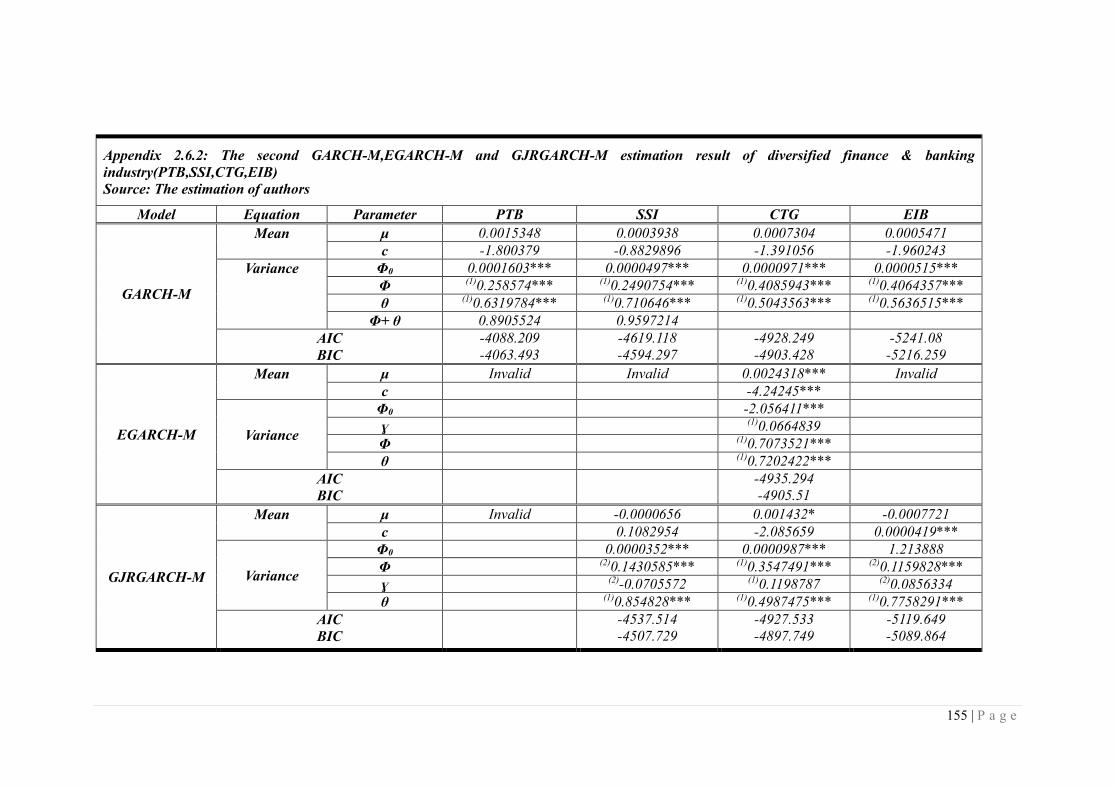
155 | P a g e

Appendix 2.6.2: The second GARCH-M,EGARCH-M and GJRGARCH-M estimation result of diversified finance & banking

industry(PTB,SSI,CTG,EIB)



GARCH-M

Mean μ 0.0015348 0.0003938 0.0007304 0.0005471

c -1.800379 -0.8829896 -1.391056 -1.960243

Variance Φ0 0.0001603*** 0.0000497*** 0.0000971*** 0.0000515***

Φ (1)0.258574*** (1)0.2490754*** (1)0.4085943*** (1)0.4064357***

θ (1)0.6319784*** (1)0.710646*** (1)0.5043563*** (1)0.5636515***

Φ+ θ 0.8905524 0.9597214

AIC

BIC

-4088.209

-4063.493

-4619.118

-4594.297

-4928.249

-4903.428

-5241.08

-5216.259

EGARCH-M

Mean μ Invalid Invalid 0.0024318*** Invalid

c -4.24245***

Variance

Φ0 -2.056411***

ɣ (1)0.0664839

Φ (1)0.7073521***

θ (1)0.7202422***

AIC

BIC

-4935.294

-4905.51

GJRGARCH-M

Mean μ Invalid -0.0000656 0.001432* -0.0007721

c 0.1082954 -2.085659 0.0000419***

Variance

Φ0 0.0000352*** 0.0000987*** 1.213888

Φ (2)0.1430585*** (1)0.3547491*** (2)0.1159828***

ɣ (2)-0.0705572 (1)0.1198787 (2)0.0856334

θ (1)0.854828*** (1)0.4987475*** (1)0.7758291***

AIC

BIC

-4537.514

-4507.729

-4927.533

-4897.749

-5119.649

-5089.864

156 | P a g e

Appendix 2.6.3: The second GARCH-M,EGARCH-M and GJRGARCH-M estimation result of banking industry (MBB, STB,VCB)



GARCH-M

Mean μ 0.0001749 0.0006793 0.0010474

c -0.8112964 -0.5812004 -1.232184

Variance Φ0 0.0000475*** 0.0000929*** 0.0001392***

Φ (1)0.4544222*** (1)0.4790183*** (1)0.3926413***

θ (1)0.506788*** (1)0.4739704*** (1)0.4765096***

Φ+ θ 0.9612102 0.9529887 0.8691509

AIC

BIC

-5390.044

-5365.223

-4940.168

-4915.347

-4706.188

-4681.377

EGARCH-M

Mean μ Invalid Invalid Invalid

c

Variance

Φ0

ɣ

Φ

θ

AIC

BIC

GJRGARCH-M

Mean μ 0.0011717* 0.0012479 -0.0006134

c -2.103525 -1.017222 0.5401461

Variance

Φ0 0.0000448*** 0.000094*** 0.0001374***

Φ (1)0.322977*** (1)0.4127623*** (1)0.4827653***

ɣ (1)0.2708967** (1)0.1311102 (1)-0.1931347*

θ (1)0.5161888*** (1)0.4738355*** (1)0.485359***

AIC

BIC

-5393.345

-5363.56

-4939.468

-4909.684

-4706.345

-4676.572

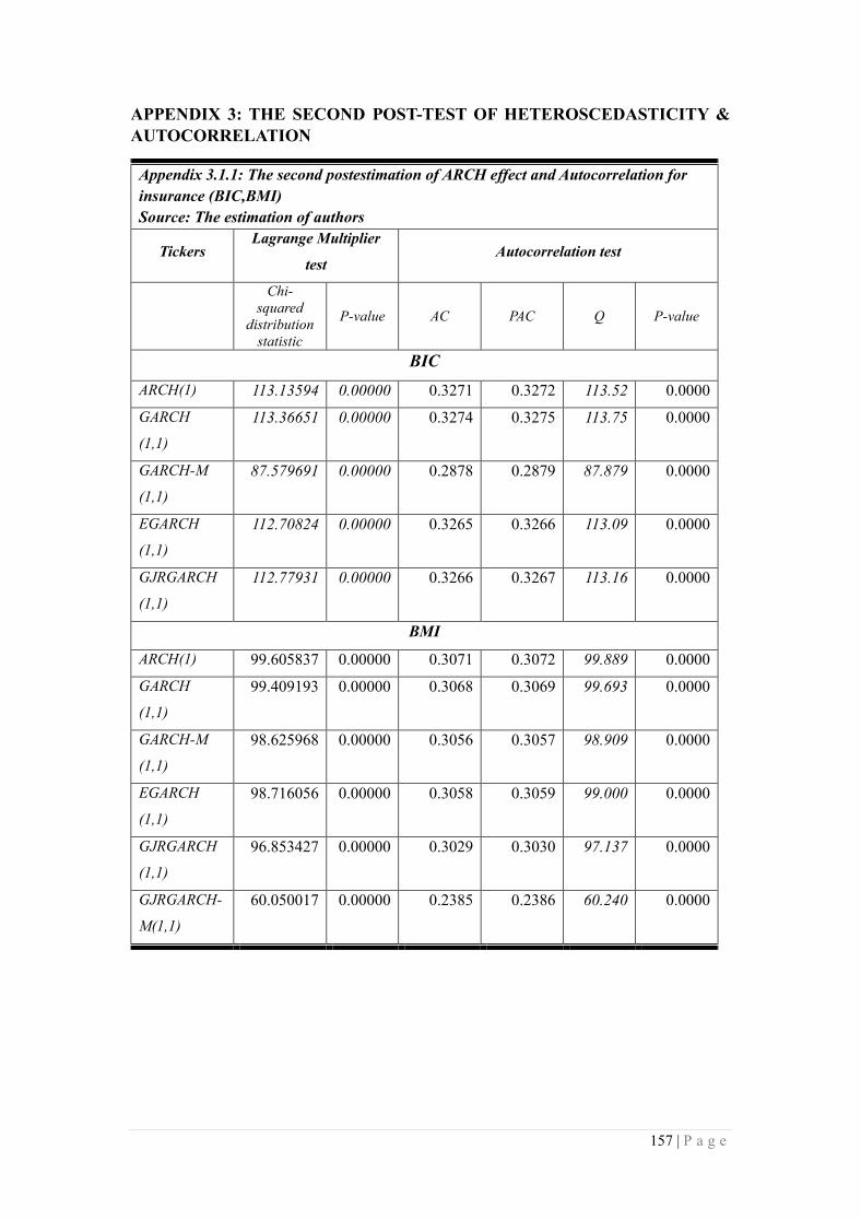
157 | P a g e

APPENDIX 3: THE SECOND POST-TEST OF HETEROSCEDASTICITY &

AUTOCORRELATION

Appendix 3.1.1: The second postestimation of ARCH effect and Autocorrelation for

insurance (BIC,BMI)



test Autocorrelation test

Chi-

squared

distribution

statistic


BIC

ARCH(1) 113.13594 0.00000 0.3271 0.3272 113.52 0.0000

GARCH

(1,1)

113.36651 0.00000 0.3274 0.3275 113.75 0.0000

GARCH-M

(1,1)

87.579691 0.00000 0.2878 0.2879 87.879 0.0000

EGARCH

(1,1)

112.70824 0.00000 0.3265 0.3266 113.09 0.0000

GJRGARCH

(1,1)

112.77931 0.00000 0.3266 0.3267 113.16 0.0000

BMI

ARCH(1) 99.605837 0.00000 0.3071 0.3072 99.889 0.0000

GARCH

(1,1)

99.409193 0.00000 0.3068 0.3069 99.693 0.0000

GARCH-M

(1,1)

98.625968 0.00000 0.3056 0.3057 98.909 0.0000

EGARCH

(1,1)

98.716056 0.00000 0.3058 0.3059 99.000 0.0000

GJRGARCH

(1,1)

96.853427 0.00000 0.3029 0.3030 97.137 0.0000

GJRGARCH-

M(1,1)

60.050017 0.00000 0.2385 0.2386 60.240 0.0000

158 | P a g e


insurance (BVH,PGI)




Chi-

squared

distribution

statistic


BVH

ARCH(1) 107.57678 0.00000 0.3190 0.3190 107.98 0.0000

GARCH

(1,1) 107.56901 0.00000 0.3190 0.3195 107.97 0.0000

GARCH-M

(1,1) 109.55871 0.00000 0.3219 0.3219 109.97 0.0000

EGARCH

(1,2) 107.25100 0.00000 0.3185 0.3185 107.65 0.0000

GJRGARCH

(1,1) 107.48008 0.00000 0.3189 0.3189 107.88 0.0000

GJRGARCH-

M(1,1) 104.91863 0.00000 0.3150 0.3151 105.31 0.0000

PGI

ARCH(1) 133.30452 0.00000 0.3647 0.3648 133.78 0.0000

GARCH

(1,1) 133.55113 0.00000 0.3650 0.3652 134.02 0.0000

GARCH-M

(1,1) 131.76101 0.00000 0.3625 0.3627 132.23 0.0000

GJRGARCH

(1,1) 131.22876 0.00000 0.3618 0.3620 131.69 0.0000

GJRGARCH-

M(1,1) 42.553718 0.00000 0.2085 0.2059 42.612 0.0000

159 | P a g e


real estate (ASM,BCI)




Chi-

squared

distribution

statistic


ASM

ARCH(2) 58.292226 0.00000 0.2348 0.2348 58.47 0.0000

GARCH

(1,1) 58.351699 0.00000 0.2349 0.2350 58.53 0.0000

GARCH-M

(1,1) 55.844683 0.00000 0.2298 0.2299 56.015 0.0000

EGARCH

(1,1) 58.375546 0.00000 0.2349 0.2350 58.554 0.0000

GJRGARCH

(1,1) 58.197396 0.00000 0.2346 0.2346 58.375 0.0000

BCI

ARCH(1) 107.05719 0.00000 0.3230 0.3231 108.29 0.0000

GARCH

(1,1) 108.1603 0.00000 0.3233 0.3234 108.50 0.0000

GARCH-M

(1,1) 113.46828 0.00000 0.3311 0.3312 113.83 0.0000

EGARCH

(1,1) 106.60534 0.00000 0.3210 0.3210 106.93 0.0000

GJRGARCH

(1,1) 105.42182 0.00000 0.3192 0.3193 105.74 0.0000

GJRGARCH-

M(1,1) 145.71634 0.00000 0.3752 0.3753 146.12 0.0000

160 | P a g e

Appendix 3.1.4:The second postestimation of ARCH effect and Autocorrelation for

real estate (CCL,CLG)




Chi-

squared

distribution

statistic


CCL

ARCH(8) 408.10289 0.00000 0.6236 0.6238 409.54 0.0000

GARCH

(1,1) 408.11005 0.00000 0.6236 0.6238 409.55 0.0000

GARCH-M

(1,1) 375.36171 0.00000 0.5981 0.5982 376.69 0.0000

EGARCH

(1,1) 408.49219 0.00000 0.6239 0.6241 409.93 0.0000

EGARCH-M

(1,1) 361.35645 0.00000 0.5868 0.5870 362.64 0.0000

GJRGARCH

(1,1) 408.50106 0.00000 0.6239 0.6241 409.94 0.0000

GJRGARCH-

M(1,1) 371.9578 0.00000 0.5954 0.5955 373.27 0.0000

CLG

ARCH(1) 46.579268 0.00000 0.2104 0.2104 46.732 0.0000

GARCH

(1,1) 46.713282 0.00000 0.2107 0.2107 46.867 0.0000

GARCH-M

(1,1) 53.496778 0.00000 0.2254 0.2255 53.671 0.0000

EGARCH

(1,1) 37.512349 0.00000 0.1888 0.1889 37.638 0.0000

GJRGARCH

(1,1) 37.661413 0.00000 0.1892 0.1892 37.788 0.0000

GJRGARCH-

M(1,1) 36.35435 0.00000 0.1859 0.1859 36.479 0.0000

161 | P a g e


real estate (D2D,DTA)




Chi-

squared

distribution

statistic


D2D

ARCH(1) 93.422896 0.00000 0.3241 0.3241 93.811 0.0000

GARCH

(1,2) 93.488798 0.00000 0.3242 0.3242 93.877 0.0000

GARCH-M

(1,2) 68.776933 0.00000 0.2781 0.2781 69.067 0.0000

EGARCH

(1,1) 92.568872 0.00000 0.3226 0.3226 92.954 0.0000

GJRGARCH

(1,2) 91.047469 0.00000 0.3200 0.3200 91.427 0.0000

DTA

ARCH(1) 76.829394 0.00000 0.2839 0.2857 76.626 0.0000

GARCH

(1,1) 76.994908 0.00000 0.2842 0.2860 76.794 0.0000

GARCH-M

(1,1) 78.286785 0.00000 0.2866 0.2883 78.131 0.0000

EGARCH

(1,1) 58.771295 0.00000 0.2481 0.2501 58.52 0.0000

GJRGARCH

(1,1) 67.935412 0.00000 0.2668 0.2688 67.686 0.0000

GJRGARCH-

M(1,1) 15.255709 0.00009 0.1269 0.1269 15.314 0.0001

162 | P a g e


real estate (DXG,FDC)




Chi-

squared

distribution

statistic


DXG

ARCH(2) 42.50002 0.00000 0.2001 0.2001 42.628 0.0000

GARCH

(1,2) 42.503579 0.00000 0.2001 0.2002 42.632 0.0000

GARCH-M

(1,2) 44.4113 0.00000 0.2045 0.2046 44.546 0.0000

EGARCH

(1,2) 42.234392 0.00000 0.1994 0.1995 42.362 0.0000

GJRGARCH

(1,2) 42.41544 0.00000 0.1999 0.1999 42.543 0.0000

FDC

ARCH(1) 84.114188 0.00000 0.3115 0.3117 84.441 0.0000

GARCH

(1,2) 84.230712 0.00000 0.3118 0.3119 84.558 0.0000

GARCH-M

(1,2) 70.992747 0.00000 0.2862 0.2863 71.269 0.0000

EGARCH

(1,2) 82.949905 0.00000 0.3094 0.3095 83.273 0.0000

GJRGARCH

(1,2) 82.597229 0.00000 0.3087 0.3088 82.919 0.0000

GJRGARCH-

M(1,2) 52.97199 0.00000 0.2472 0.2473 53.182 0.0000

163 | P a g e

Appendix 3.1.7:The second postestimation of ARCH effect and Autocorrelation for

real estate (FLC, HDC)




Chi-

squared

distribution

statistic


FLC

ARCH(1) 41.417669 0.00000 0.1980 0.1981 41.556 0.0000

GARCH

(1,1) 41.475119 0.00000 0.1981 0.1982 41.614 0.0000

GARCH-M

(1,1) 36.866821 0.00000 0.1868 0.1869 36.991 0.0000

EGARCH

(1,1) 39.867947 0.00000 0.1943 0.1943 40.002 0.0000

GJRGARCH

(1,1) 41.34035 0.00000 0.1978 0.1979 41.478 0.0000

HDC

ARCH(1) 114.19869 0.00000 0.3374 0.3375 114.15 0.0000

GARCH

(1,1) 114.24011 0.00000 0.3374 0.3375 114.19 0.0000

GARCH-M

(1,1) 111.69427 0.00000 0.3336 0.3337 111.64 0.0000

GJRGARCH

(1,1) 113.53857 0.00000 0.3364 0.3365 113.48 0.0000

GJRGARCH-

M(1,1) 114.05429 0.00000 0.3371 0.3373 113.99 0.0000

164 | P a g e


real estate (HQC,ITC)




Chi-

squared

distribution

statistic


HQC

ARCH(1) 52.557587 0.00000 0.2225 0.2226 52.742 0.0000

GARCH

(1,1) 52.568679 0.00000 0.2226 0.2226 52.753 0.0000

GARCH-M

(1,1) 52.594137 0.00000 0.2226 0.2227 52.778 0.0000

GJRGARCH

(1,1) 52.56852 0.00000 0.2226 0.2226 52.753 0.0000

ITC

ARCH(1) 79.404812 0.00000 0.2736 0.2736 79.700 0.0000

GARCH

(1,2) 77.43349 0.00000 0.2701 0.2701 77.723 0.0000

GARCH-M

(1,2) 77.10918 0.00000 0.2702 0.2702 77.738 0.0000

EGARCH

(1,1) 75.834945 0.00000 0.2673 0.2673 76.119 0.0000

GJRGARCH

(1,1) 77.045505 0.00000 0.2695 0.2695 77.333 0.0000

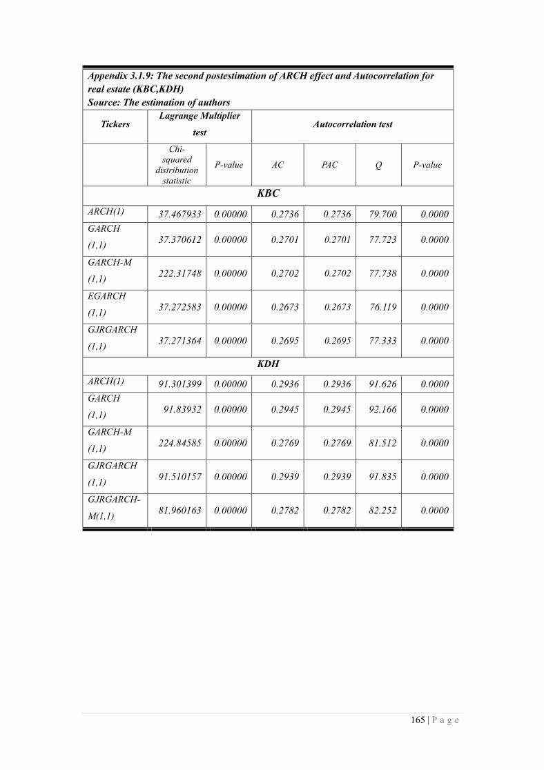
165 | P a g e


real estate (KBC,KDH)




Chi-

squared

distribution

statistic


KBC

ARCH(1) 37.467933 0.00000 0.2736 0.2736 79.700 0.0000

GARCH

(1,1) 37.370612 0.00000 0.2701 0.2701 77.723 0.0000

GARCH-M

(1,1) 222.31748 0.00000 0.2702 0.2702 77.738 0.0000

EGARCH

(1,1) 37.272583 0.00000 0.2673 0.2673 76.119 0.0000

GJRGARCH

(1,1) 37.271364 0.00000 0.2695 0.2695 77.333 0.0000

KDH

ARCH(1) 91.301399 0.00000 0.2936 0.2936 91.626 0.0000

GARCH

(1,1) 91.83932 0.00000 0.2945 0.2945 92.166 0.0000

GARCH-M

(1,1) 224.84585 0.00000 0.2769 0.2769 81.512 0.0000

GJRGARCH

(1,1) 91.510157 0.00000 0.2939 0.2939 91.835 0.0000

GJRGARCH-

M(1,1) 81.960163 0.00000 0.2782 0.2782 82.252 0.0000

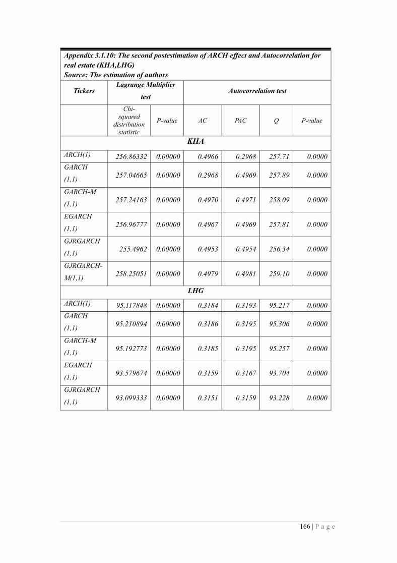
166 | P a g e


real estate (KHA,LHG)




Chi-

squared

distribution

statistic


KHA

ARCH(1) 256.86332 0.00000 0.4966 0.2968 257.71 0.0000

GARCH

(1,1) 257.04665 0.00000 0.2968 0.4969 257.89 0.0000

GARCH-M

(1,1) 257.24163 0.00000 0.4970 0.4971 258.09 0.0000

EGARCH

(1,1) 256.96777 0.00000 0.4967 0.4969 257.81 0.0000

GJRGARCH

(1,1) 255.4962 0.00000 0.4953 0.4954 256.34 0.0000

GJRGARCH-

M(1,1) 258.25051 0.00000 0.4979 0.4981 259.10 0.0000

LHG

ARCH(1) 95.117848 0.00000 0.3184 0.3193 95.217 0.0000

GARCH

(1,1) 95.210894 0.00000 0.3186 0.3195 95.306 0.0000

GARCH-M

(1,1) 95.192773 0.00000 0.3185 0.3195 95.257 0.0000

EGARCH

(1,1) 93.579674 0.00000 0.3159 0.3167 93.704 0.0000

GJRGARCH

(1,1) 93.099333 0.00000 0.3151 0.3159 93.228 0.0000

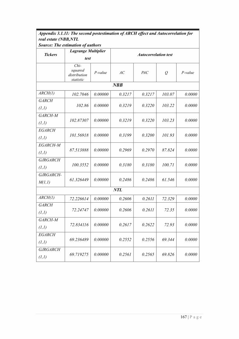
167 | P a g e


real estate (NBB,NTL




Chi-

squared

distribution

statistic


NBB

ARCH(1) 102.7046 0.00000 0.3217 0.3217 103.07 0.0000

GARCH

(1,1) 102.86 0.00000 0.3219 0.3220 103.22 0.0000

GARCH-M

(1,1) 102.87307 0.00000 0.3219 0.3220 103.23 0.0000

EGARCH

(1,1) 101.56918 0.00000 0.3199 0.3200 101.93 0.0000

EGARCH-M

(1,1) 87.513888 0.00000 0.2969 0.2970 87.824 0.0000

GJRGARCH

(1,1) 100.3552 0.00000 0.3180 0.3180 100.71 0.0000

GJRGARCH-

M(1,1) 61.326449 0.00000 0.2486 0.2486 61.546 0.0000

NTL

ARCH(1) 72.226614 0.00000 0.2606 0.2611 72.329 0.0000

GARCH

(1,1) 72.24747 0.00000 0.2606 0.2611 72.35 0.0000

GARCH-M

(1,1) 72.834116 0.00000 0.2617 0.2622 72.93 0.0000

EGARCH

(1,1) 69.236489 0.00000 0.2552 0.2556 69.344 0.0000

GJRGARCH

(1,1) 69.719275 0.00000 0.2561 0.2565 69.826 0.0000

168 | P a g e

Appendix 3.1.12: The second Postestimation of ARCH effect and Autocorrelation for

real estate (NVT,PDR)




Chi-

squared

distribution

statistic


NVT

ARCH(1) 60.524207 0.00000 0.2401 0.2402 60.695 0.0000

GARCH

(1,1) 60.528398 0.00000 0.2401 0.2402 60.700 0.0000

GARCH-M

(1,1) 65.111983 0.00000 0.2490 0.2491 65.296 0.0000

EGARCH

(1,1) 60.315857 0.00000 0.2397 0.2398 60.486 0.0000

GJRGARCH

(1,1) 59.159445 0.00000 0.2374 0.2375 59.327 0.0000

GJRGARCH-

M(1,1) 18.16927 0.00002 0.1316 0.1316 18.225 0.0000

PDR

ARCH(3) 141.88487 0.00000 0.3926 0.3927 142.42 0.0000

GARCH

(1,2) 141.95895 0.00000 0.3927 0.3928 142.49 0.0000

GARCH-M

(1,2) 153.28577 0.00000 0.4081 0.4082 153.86 0.0000

GJRGARCH

(1,2) 138.52209 0.00000 0.3879 0.3880 139.04 0.0000

GJRGARCH-

M(1,2) 119.52605 0.00000 0.3603 0.3604 119.97 0.0000

169 | P a g e


real estate (PTL,QCG)




Chi-

squared

distribution

statistic


PTL

ARCH(1) 33.745884 0.00000 0.1784 0.1785 33.845 0.0000

GARCH

(1,1) 33.769855 0.00000 0.1785 0.1786 33.869 0.0000

GARCH-M

(1,1) 35.118292 0.00000 0.1820 0.1821 35.221 0.0000

EGARCH

(1,1) 30.273756 0.00000 0.1690 0.1691 30.365 0.0000

EGARCH-M

(1,1) 33.670025 0.00000 0.1782 0.1783 33.769 0.0000

GJRGARCH

(1,1) 30.365394 0.00000 0.1693 0.1694 30.457 0.0000

QCG

ARCH(1) 81.380038 0.00000 0.2767 0.2771 81.566 0.0000

GARCH

(1,1) 81.369916 0.00000 0.2767 0.2771 81.554 0.0000

GARCH-M

(1,1) 79.949695 0.00000 0.2743 0.2747 80.137 0.0000

EGARCH

(1,1) 81.344918 0.00000 0.2767 0.2771 81.528 0.0000

GJRGARCH

(1,1) 81.380105 0.00000 0.2767 20.2771 81.565 0.0000

GJRGARCH-

M(1,1) 69.942671 0.00000 0.2566 0.2569 70.112 0.0000

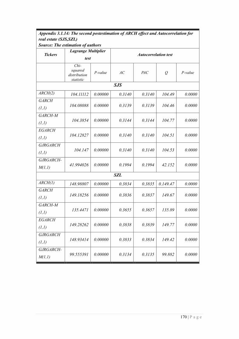
170 | P a g e


real estate (SJS,SZL)




Chi-

squared

distribution

statistic


SJS

ARCH(2) 104.11112 0.00000 0.3140 0.3140 104.49 0.0000

GARCH

(1,1) 104.08088 0.00000 0.3139 0.3139 104.46 0.0000

GARCH-M

(1,1) 104.3854 0.00000 0.3144 0.3144 104.77 0.0000

EGARCH

(1,1) 104.12827 0.00000 0.3140 0.3140 104.51 0.0000

GJRGARCH

(1,1) 104.147 0.00000 0.3140 0.3140 104.53 0.0000

GJRGARCH-

M(1,1) 41.994026 0.00000 0.1994 0.1994 42.152 0.0000

SZL

ARCH(1) 148.98807 0.00000 0.3834 0.3835 0.149.47 0.0000

GARCH

(1,1) 149.18256 0.00000 0.3836 0.3837 149.67 0.0000

GARCH-M

(1,1) 135.4471 0.00000 0.3655 0.3657 135.89 0.0000

EGARCH

(1,1) 149.28262 0.00000 0.3838 0.3839 149.77 0.0000

GJRGARCH

(1,1) 148.93414 0.00000 0.3833 0.3834 149.42 0.0000

GJRGARCH-

M(1,1) 99.555391 0.00000 0.3134 0.3135 99.882 0.0000

171 | P a g e

Appendix 3.1.12: Postestimation of ARCH effect and Autocorrelation for real estate

(CIG,TDH)




Chi-

squared

distribution

statistic


CIG

ARCH(1) 33.413326 0.00000 0.1795 0.1795 33.525 0.0000

GARCH

(1,1) 33.317342 0.00000 0.1792 0.1792 33.429 0.0000

GARCH-M

(1,1) 29.054231 0.00000 0.1673 0.1673 29.151 0.0000

EGARCH

(1,1) 24.912946 0.00000 0.1550 0.1550 24.995 0.0000

GJRGARCH

(1,1) 33.254289 0.00000 0.1790 0.1790 33.365 0.0000

GJRGARCH-

M(1,1) 25.860773 0.00000 0.1752 0.1752 33.884 0.0000

TDH

ARCH(1) 52.514996 0.00000 0.2224 0.2224 52.687 0.0000

GARCH

(1,1) 52.511412 0.00000 0.2224 0.2224 52.684 0.0000

GARCH-M

(1,1) 53.237182 0.00000 0.2240 0.2240 53.415 0.0000

EGARCH

(1,1) 52.42186 0.00000 0.2240 0.2240 53.415 0.0000

GJRGARCH

(1,1) 51.605015 0.00000 0.2205 0.2205 51.773 0.0000

172 | P a g e


(TIX,VIC)




Chi-

squared

distribution

statistic


TIX

ARCH(2) 128.26604 0.00000 0.3959 0.3960 128.84 0.0000

GARCH

(1,1) 128.86952 0.00000 0.3968 0.3969 129.44 0.0000

GARCH-M

(1,1) 128.21681 0.00000 0.3958 0.3959 128.78 0.0000

EGARCH

(1,1) 127.40109 0.00000 0.3946 0.3946 127.97 0.0000

GJRGARCH

(1,1) 128.34264 0.00000 0.3960 0.3961 128.91 0.0000

GJRGARCH-

M(1,1) 129.85227 0.00040 0.3983 0.3984 130.42 0.0000

VIC

ARCH(1) 169.58346 0.00070 0.3996 0.3997 169.75 0.0007

GARCH

(1,1) 169.76349 0.00000 0.3998 0.3999 169.92 0.0007

GARCH-M

(1,1) 170.4357 0.00000 0.4007 0.4008 170.71 0.0006

EGARCH

(1,1) 170.01752 0.00000 0.4001 0.4001 170.13 0.0007

GJRGARCH

(1,1) 170.10343 0.00000 0.4002 0.4002 170.24 0.0007

GJRGARCH-

M(1,1) 174.08537 0.00000 0.4050 0.4050 174.34 0.0007

173 | P a g e


(VPH,DRH)




Chi-

squared

distribution

statistic


VPH

ARCH(1) 53.725566 0.00853 0.2239 0.2240 53.278 0.0084

GARCH

(1,1) 53.843665 0.00837 0.2241 0.2242 53.393 0.0083

GARCH-M

(1,1) 51.637759 0.00955 0.2195 0.2196 51.220 0.0094

EGARCH

(1,1) 52.972161 0.00881 0.2223 0.2224 52.545 0.0087

GJRGARCH

(1,1) 49.087517 0.00908 0.2141 0.2142 48.739 0.0017

GJRGARCH-

M(1,1) 31.55458 0.00929 0.1714 0.1715 0.31226 0.0017

DRH

ARCH(1) 21.131202 0.00000 0.1431 0.1432 21.204 0.0000

GARCH

(1,1) 21.127267 0.00000 0.1431 0.1432 21.200 0.0000

GARCH-M

(1,1) 21.04321 0.00000 0.1428 0.1429 21.116 0.0000

EGARCH

(1,1) 15.516953 0.00000 0.1227 0.1227 15.571 0.0001

GJRGARCH

(1,1) 20.669072 0.00000 0.1416 0.1416 20.742 0.0000

GJRGARCH-

M(1,1) 20.189790 0.00000 0.1796 0.1796 21.551 0.0000

174 | P a g e


Diversified finance group (AGR, BSI)



Chi-

squared

distribution

statistic

P-value Critical


AGR ARCH(1)

94.2452 0.000 3.840 0.2981 0.2984 94.281 0.000

GARCH

(1,1) 94.3036 0.000 3.841 0.2982 0.2985 94.34 0.000

GARCH-

M(1,1) 96.406 0.000 3.844 0.3015 0.3019 96.472 0.000

EGARCH(1,1) 91.728 0.000 3.814 0.2941 0.2944 91.757 0.000

EGARCH

-M(2,1) 91.613 0.000 3.841 0.2939 0.2942 91.656 0.000

TGARCH

(1,1) 90.401 0.000 3.854 0.2919 0.2922 90.427 0.000

TGARCH-M(1,1) 90.722 0.000 3.814 0.1322 0.1326 90.555 0.000

BSI ARCH(1)

36.522 0.000 3.848 0.1859 0.1860 36.639 0.000

GARCH

(1,1) 36.725 0.000 3.840 0.1864 0.1865 36.843 0.000

GARCH-M(1,1) 36.538 0.000 3.828 0.1860 0.1860 36.655 0.000

EGARCH

(1,1) 25.501 0.000 3.841 0.1554 0.1554 25.584 0.000

EGARCH

-M(2,1) 24.272 0.000 3.811 0.1516 0.1516 24.359 0.000

TGARCH(1,1) 33.189 0.000 3.811 0.1772 0.1772 33.286 0.000

TGARCH

-M(1,1) 23.288 0.0021 3.884 0.1070 0.1708 15.305 0.000

175 | P a g e


Diversified finance group (HCM, OGC)



Chi-

squared

distribution

statistic

P-value Critical


HCM

ARCH(1) 82.248 0.000 3.848 0.2790 0.2790 82.52 0.000

GARCH

(1,1) 82.309 0.000 3.840 0.2790 0.2791 82.58 0.000

GARCH-M(1,1) 82.2956 0.000 3.841 0.2790 0.2790 82.57 0.000

EGARCH

(1,1) 82.213 0.000 3.840 0.2790 0.2791 82.59 0.000

EGARCH

-M(1,1) 65.787 0.000 3.811 0.2494 0.2495 66.01 0.000

TGARCH(1,1) 82.299 0.000 3.841 0.2790 0.2790 82.573 0.000

TGARCH

-M(1,1) 78.948 0.000 3.884 0.2732 0.2733 79.211 0.000

OGC

ARCH(1) 39.505 0.000 3.840 0.1933 0.1933 39.635 0.000

GARCH

(1,1) 39.514 0.000 3.844 0.1933 0.1933 39.643 0.000

GARCH-

M(1,1) 39.661 0.000 3.840 0.1937 0.1937 39.789 0.000

EGARCH

(1,2) 39.514 0.000 3.841 0.1933 0.1933 39.644 0.000

TGARCH

(1,1) 39.075 0.000 3.841 0.1922 0.1922 39.204 0.000

176 | P a g e

Appendix 3.2.3: The second postestimation of ARCH effect and Autocorrelation for Diversified

finance group (PTB, SSI)



Chi-

squared

distribution

statistic

P-value Critical


PTB

ARCH(1) 73.279 0.000 3.841 0.2657 0.2658 73.361 0.000

GARCH

(1,1) 73.190 0.000 3.841 0.2656 0.2656 73.271 0.000

GARCH-

M(1,1) 77.898 0.000 3.811 0.2740 0.2741 77.996 0.000

EGARCH(1,1) 71.061 0.000 3.804 0.2616 0.2617 71.124 0.000

TGARCH

(1,1) 70.777 0.000 3.840 0.2611 0.2612 70.839 0.000

SSI

ARCH(1) 128.126 0.000 3.840 0.3481 0.3481 128.54 0.000

GARCH (1,1) 128.112 0.000 3.840 0.3481 0.3481 128.53 0.000

GARCH-

M(1,1) 122.384 0.000 3.840 0.3402 0.3403 122.78 0.000

EGARCH(1,1) 126.719 0.000 3.840 0.3462 0.3462 127.13 0.000

TGARCH

(2,1) 128.088 0.000 3.880 0.3480 0.3481 128.51 0.000

TGARCH

-M(2,1) 128.299 0.000 3.840 0.3483 0.3484 128.72 0.000

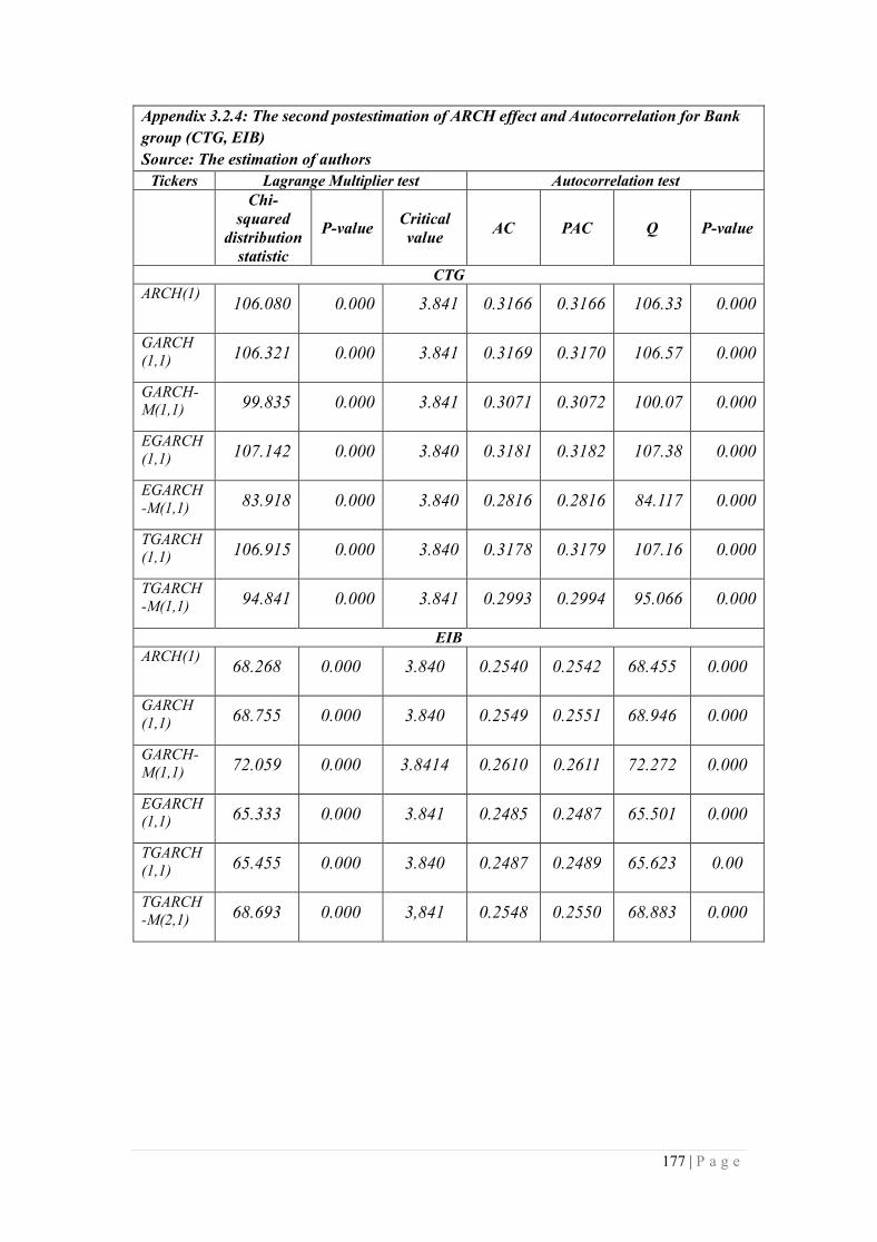
177 | P a g e

Appendix 3.2.4: The second postestimation of ARCH effect and Autocorrelation for Bank

group (CTG, EIB)



Chi-

squared

distribution

statistic

P-value Critical


CTG

ARCH(1) 106.080 0.000 3.841 0.3166 0.3166 106.33 0.000

GARCH

(1,1) 106.321 0.000 3.841 0.3169 0.3170 106.57 0.000

GARCH-M(1,1) 99.835 0.000 3.841 0.3071 0.3072 100.07 0.000

EGARCH

(1,1) 107.142 0.000 3.840 0.3181 0.3182 107.38 0.000

EGARCH

-M(1,1) 83.918 0.000 3.840 0.2816 0.2816 84.117 0.000

TGARCH(1,1) 106.915 0.000 3.840 0.3178 0.3179 107.16 0.000

TGARCH

-M(1,1) 94.841 0.000 3.841 0.2993 0.2994 95.066 0.000

EIB

ARCH(1) 68.268 0.000 3.840 0.2540 0.2542 68.455 0.000

GARCH

(1,1) 68.755 0.000 3.840 0.2549 0.2551 68.946 0.000

GARCH-

M(1,1) 72.059 0.000 3.8414 0.2610 0.2611 72.272 0.000

EGARCH(1,1) 65.333 0.000 3.841 0.2485 0.2487 65.501 0.000

TGARCH

(1,1) 65.455 0.000 3.840 0.2487 0.2489 65.623 0.00

TGARCH

-M(2,1) 68.693 0.000 3,841 0.2548 0.2550 68.883 0.000

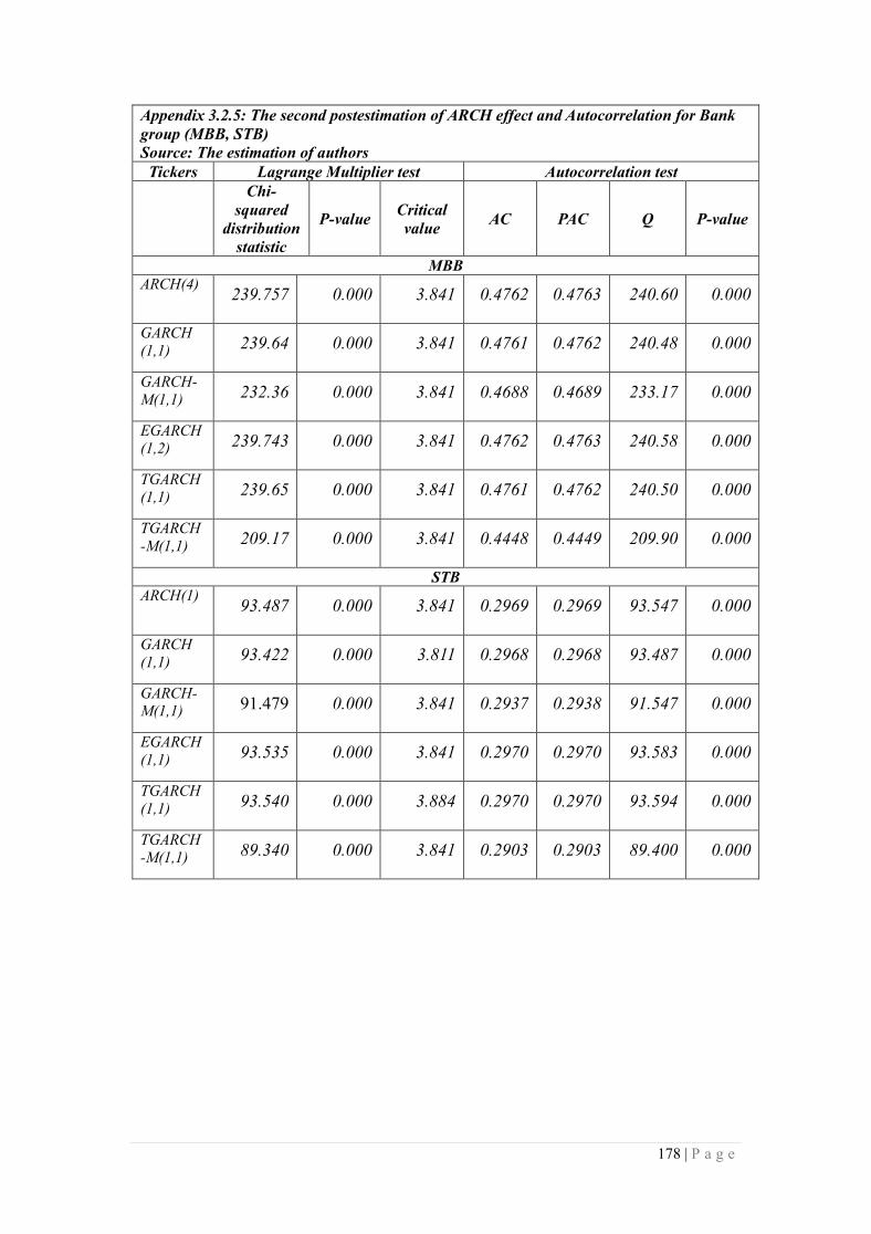
178 | P a g e


group (MBB, STB)


Tickers Lagrange Multiplier test Autocorrelation test Chi-

squared

distribution

statistic

P-value Critical


MBB

ARCH(4) 239.757 0.000 3.841 0.4762 0.4763 240.60 0.000

GARCH

(1,1) 239.64 0.000 3.841 0.4761 0.4762 240.48 0.000

GARCH-

M(1,1) 232.36 0.000 3.841 0.4688 0.4689 233.17 0.000

EGARCH(1,2) 239.743 0.000 3.841 0.4762 0.4763 240.58 0.000

TGARCH

(1,1) 239.65 0.000 3.841 0.4761 0.4762 240.50 0.000

TGARCH

-M(1,1) 209.17 0.000 3.841 0.4448 0.4449 209.90 0.000

STB

ARCH(1) 93.487 0.000 3.841 0.2969 0.2969 93.547 0.000

GARCH

(1,1) 93.422 0.000 3.811 0.2968 0.2968 93.487 0.000

GARCH-M(1,1) 91.479 0.000 3.841 0.2937 0.2938 91.547 0.000

EGARCH

(1,1) 93.535 0.000 3.841 0.2970 0.2970 93.583 0.000

TGARCH

(1,1) 93.540 0.000 3.884 0.2970 0.2970 93.594 0.000

TGARCH-M(1,1) 89.340 0.000 3.841 0.2903 0.2903 89.400 0.000

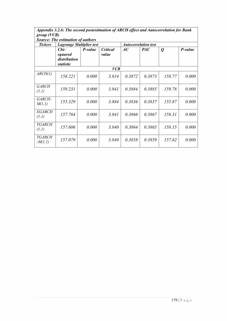
179 | P a g e


group (VCB)



Chi-

squared

distribution

statistic

P-value Critical

value

AC PAC Q P-value

VCB

ARCH(1) 158.221 0.000 3.814 0.3872 0.3873 158.77 0.000

GARCH

(1,1) 159.231 0.000 3.841 0.3884 0.3885 159.78 0.000

GARCH-

M(1,1) 155.329 0.000 3.884 0.3836 0.3837 155.87 0.000

EGARCH(1,1) 157.764 0.000 3.841 0.3866 0.3867 158.31 0.000

TGARCH(1,1) 157.606 0.000 3.840 0.3864 0.3865 158.15 0.000

TGARCH

-M(1,1) 157.079 0.000 3.840 0.3858 0.3859 157.62 0.000

180 | P a g e

REFERENCES

A.Angabini and S.Wasiuzzaman, 2011, “GARCH models and the Financial crisis – A

study of the Malaysian stock markets”, The international Journal of Apllied

Economics and Finance 5(3), p.226-236 (ISSN: 1991-0886)

Afees A.Salisu & Ismail O.Fasanya, 2012, “Comparative performance of volatility

models for oil price”, International Journal of Energy Economics and Policy,

Vol.2, No.3, p.167-183 (ISSN: 2146-4553)

Ching Mun Lim & Siok Kun Sek, 2013, “Comparing the performmaces of GARCH-

type models in capturing the stock market volatility in Malaysia”, Procedia

Economics and Finance 5, p.478-487

Dana Al-Najjar, 2016, “Modelling and estimation of volatility using ARCH/GARCH

models in Jordan’s stock market”, Asian Journal of Finance & Accounting, Vo.8,

No.1, p.152-167 (ISSN:1946-052X)

Daniel B.Nelson, 1991, “Conditional Heteroscedasticity in asset returns: A new

approach”, Econometrica, Vol.59, No.2, p.347-370

Dima Elberg, Haim Shalit & Rami Yosef, 2008, “Estimating stock market volatility

using asymmetric GARCH models”, Applied Financial Economics 18, p.1201-

1208

David G.McMillan * Alan E.H.Speight, 2004, “Daily volatility forecasts: Reassessing

the performance of GARCH models”, Journal of Forecasting 23, p.449-460

Emenike Kalu O. & Aleke Stephen Friday, 2012, “Modeling Asymmetric volatility in

the Nigerian Stock Exchange”, European Journal of Business and Mangement,

Vol.4, No.12 (ISSN: 2222-1905)

Fethi Belhaj & Ezzeddine Abaoub, 2015, “A GARCH examination of the relationship

between trading volum and conditional volatility in the Tunisian stock market:

Evidence for the Information Flow Paradigm”, International Journal of

Economics and Financial Issues 5(2), p.354-364 (ISSN: 2146-4138).

Frimpong Joseph Magnus & Oteng-Abayie Eric Fosu, 2006, “Modelling and

forecasting volatility of returns on the Ghana stock exchange using GARCH

models”, American Journal of Applied Sciences 3 (10, ISSN: 1546-9239,

p.2042-2048

181 | P a g e

Heping Liu & Jing Shi, 2013, “Applying ARMA-GARCH approaches to forecasting

short-term electricity prices”, Energy Economics 37, p.152-166

Lawrence R.Glosten, Ravi Jagannathan & David E.Runkle, 1993, “On the relation

between the expected value and the volatility of the nomial excess return on

stocks”, The Journal of Finance, Vol.48, No.5, p.1779-1801

Mohd Aminul Islem, 2013, “Estimating volatility of stock index returns by using

Symmetric GARCH models”, Middle-East Journal of Scientific Research 18 (7),

p.991-999

Mohd. Aminul Islam, 2013, “Modeling Univariate volatility of stock returns using

Stochastic GARCH models: Evidence from 4-Asian markets”, Australian

Journal of Basic and Apllied Sciences 7 (11), p.294-303

M.Tamilselvan & Shaik Mastan Vali, 2016, “Forecasting stock market volatility –

Evidence from Muscat security market using GARCH models”, International

Journal of Commerce and Finance, Vol.2, Issue 1, p.37-53

Philip Hans Franses & Dick Van Dijk, 1996, “Forecasting Stock Market Volatility

using Non-linear GARCH models”, Journal of Forecasting, Vol.15, p.229-235

R.Ilker Gokbulut & Mehmet Pekkaya, 2014, “Estimating and forecasting volatility of

financial market using Asymmetric GARCH models: An application on Turkish

Financial Markets”, International Journal of Economics and Finance, Vol.6, No.4,

p.23-35 (ISSN: 1916-971X)

Robert F.Engle & Victor K.Ng, 1993, “Measuring and testing the impact of news on

volatility”, The Journal of Finance, Vol.48, No.5, p.1749-1778

Robert F.Engle, 1982, “Autoregressive Conditional Heteroscedasticity with Estimates

of the Variance of United Kingdom Inflation”, Econometrica, Vol.50, Issue 4,

p.987-1008

Robert F.Engle, David M.Lilien and Russell P.Robin, 1987, “Estimating time-varying

risk premia in the term structure: The ARCH-M model”, Econometrica, Vol.55,

Issue.2, p.391-407

Sohail Chand, Shahid Kamal & Imran Ali, 2012, “Modeling and Volatility analysis of

share prices using ARCH and GARCH models”, World Applied Sciences Journal

19 (1), p.77-82 (ISSN: 1818-4952)

182 | P a g e

Suliman Zakaria & Peter Winker, 2012, “Modelling stock market volatility using

Univariate GARCH models: Evidence from Sudan and Egypt”, International

Journal of Economics and Finance, Vol.4, No.8, p.161-176

Ser-Huang Poon & Clive W.J.Granger, 2003, “Forecasting volatility in financial

markets: A reivew”, Journal of Economic Literature, Vol.41, No.2, p.478-539

Tim Bollerslev, 2007, “Glossary to ARCH (GARCH)”, p.4-16

Tim Bollerslev, 1986, “Generalized Autoregressive Conditional Heteroscedasticity”,

Journal of Econometric 31, p.307-327

Tim Bollerslev, Ray Y.Chou & Kenneth F.Kroner, 1992, “ARCH modeling in finance

– A review of the theory and empirical evidence”, Journal of Econometrics 52,

p.5-59

Trilochan Tripathy & Luis A.Gil Alana, 2015, “Modelling time-varying volatility in

the Indian stock returns: Some empirical evidence”, Review of Development 5,

p.91-97

stock return volatility modeling by using...

Documents