38th annual progress report june 2017 chapter 4...

Methodology for Flow and Salinity Estimates in the Sacramento-San Joaquin Delta and Suisun Marsh

38th Annual Progress Report June 2017

Chapter 4

Clifton Court Forebay Transit Time Modeling Analysis Authors: Qiang Shu, Eli Ateljevich

Bay-Delta Office Delta Modeling Section Department of Water Resources

Methodology for Flow and Salinity Estimates 38th Annual Progress Report

Clifton Court Forebay Transit Time Modeling Analysis -i

Contents

Contents

4. Clifton Court Forebay Transit Time Modeling Analysis ................................................................... 4-1

4.1 INTRODUCTION ................................................................................................................................. 4-1 4.1.1 Site Characterization ................................................................................................................ 4-1

4.2 MODEL DESCRIPTION ........................................................................................................................... 4-7

4.2.1 Hydrodynamics ........................................................................................................................ 4-7 4.2.2 Radial Gate Parameterization ................................................................................................... 4-8 4.2.2.1 Evaporation ...................................................................................................................... 4-8 4.2.3 Particle Tracking ...................................................................................................................... 4-8 4.2.4 Mesh and Time Discretization ................................................................................................. 4-9 4.3 INPUT DATA SOURCES.................................................................................................................... 4-11 4.3.1 Banks Pumping Plant Flow .................................................................................................... 4-11 4.3.2 Radial Gate Operations .......................................................................................................... 4-11 4.3.3 Bathymetry ............................................................................................................................. 4-11 4.3.4 Wind ....................................................................................................................................... 4-11

4.4 CALIBRATION AND VALIDATION ....................................................................................................... 4-13

4.5 TRANSIT TIME AND VELOCITY ANALYSIS ......................................................................................... 4-21

4.5.1 Dredge and Fill Alternatives .................................................................................................. 4-21 4.5.2 Methods.................................................................................................................................. 4-21 4.5.3 Key Results ............................................................................................................................ 4-24 4.5.3.1 Patterns and Variations in Particle Trajectories ............................................................. 4-24 4.5.4 Transit Time ........................................................................................................................... 4-27

4.6 DISCUSSION ........................................................................................................................................ 4-30

4.7 REFERENCES CITED ............................................................................................................................ 4-33

4.7.1 Personal Communications...................................................................................................... 4-34

Figures Figure 4-1 Location and Aerial View of Clifton Court Gates 4-2

Figure 4-2 Bathymetric Map of Clifton Court Forebay ........................................................................................ 4-3

Figure 4-3 Priority Schedules Describing the Eligible Periods for Opening Clifton Court Radial Gates ......... 4-4

Figure 4-4 Skinner Delta Fish Protection Facility ................................................................................................. 4-6

Figure 4-5 Horizontal Mesh ................................................................................................................................. 4-10

Figure 4-6 U.S. Geological Survey Sampling Locations for Upward-looking ADCPs and Drifters .............. 4-14

Figure 4-7 Sketch of Upward-Looking ADCP Beam and Sampling Bins ....................................................... 4-14

Figure 4-8 Boundary Flows and Wind (top) and Comparisons with Observed Velocity at Site CCFWE .... 4-15


Page 4-ii Clifton Court Forebay Transit Time Modeling Analysis

Figure 4-9 Boundary Flows and Wind (top) and Comparisons with Observed Velocity at Site CCFNE ..... 4-16

Figure 4-10 Boundary Flows and Wind (top) and Comparisons with Observed Velocity at Site CCFSC .... 4-17

Figure 4-11 Boundary Flows and Wind (top) and Comparisons with Observed Velocity at Site CCFCS .... 4-18

Figure 4-12 Boundary Flows and Wind (top) and Comparisons with Observed Velocity at Site CCFNO ... 4-19

Figure 4-13 Boundary Flows and Wind (top) and Comparisons with Observed Velocity at site CCFCN .... 4-20

Figure 4-14 Base Case and Dredging and Filling Options Explored in This Report ........................................ 4-22

Figure 4-15 Radial Gate Flow, Banks Intake Flow, and Wind Conditions for 2012 (top), 2016 (middle), and 2017 (bottom) .............................................................................................................................. 4-23

Figure 4-16 Particle Trajectories and Velocity Gradients in Low Flow Under Three Bathymetry Options .. 4-25

Figure 4-17 Particle Trajectories and Velocity Gradients in High Flow Under Three Bathymetry Options . 4-26

Figure 4-18 Retention Curves for Base and Filling Options, Low-Flow (2016) Case ..................................... 4-28

Figure 4-19 Retention Curves for Base and Dredge + Fill Options, Low-Flow (2016) Case .. 4-Error! Bookmark not defined.

Figure 4-19 Retention Curves for Base and Dredge + Fill Options, Low-Flow (2016) Case .......................... 4-28

Figure 4-20 Retention Curves for Base and Dredge + Fill Options, High-Flow (2012) Case ......................... 4-29

Figure 4-21 Retention Curves for Base Bathymetry in Low-medium Flow (2016), Medium-High Flow (2012), and Extreme High Flow (2017) ........................................................................................... 4-29


Clifton Court Forebay Transit Time Modeling Analysis Page 4-1

4. Clifton Court Forebay Transit Time Modeling Analysis 4.1 Introduction This chapter is excerpted from Shu and Ateljevich (2017), referred to from this point on as the “Report,” and summarizes 3D hydrodynamic modeling performed by the California Department of Water Resources’ (DWR’s) Bay-Delta Office (BDO) to assess flow patterns and transit time in the Clifton Court Forebay (Forebay). The motivation for this work comes from the National Marine Fisheries Service 2009 Biological Opinion, Action IV.4.2 (National Marine Fisheries Service 2011), which prescribes limits on pre-screen losses of salmonids and steelhead in the Forebay and obliges DWR to study methods to reduce this loss. The Report focuses on model development that has been completed and a study based on this model of how transit time across the Forebay responds to various filling and dredging actions. The premise underlying this investigation is that fish will benefit from faster transit, which reduces their exposure to predators.

The Report characterizes the site, model formulation, and validation on field data. It supports the following findings:

1. Filling scour areas near the Clifton Court radial gates reduces transit time and enhances the benefits of dredging options.

2. Some dredging actions reduce transit time significantly when combined with filling of scour areas. 3. Transit time is more sensitive to flow operations than bathymetry. 4. The transit time interventions that are most effective and straightforward to model operate by

shortening primary particle trajectories in the first few 2–5 days after entry.

The Report does not address engineering and design concerns or the morphological stability of the proposed bathymetry alterations.

4.1.1 Site Characterization

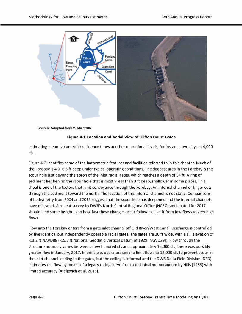
Clifton Court Forebay was completed in 1969. Located in the southern portion of the Sacramento-San Joaquin Delta (Delta) (Figure 4-1), the Forebay is a regulating reservoir that serves as a buffer between diversions from the Delta and State Water Project (SWP) pumping at the Harvey O. Banks Pumping Plant (Banks Pumping Plant). The Forebay affords DWR operators flexibility in meeting daily allocations, preserving sufficient water levels for south Delta agricultural diversions, and scheduling pumping around diurnal fluctuations in electricity prices. With an area of 2,200 acres (97.5 million square feet [sq ft]), an average depth of 7 feet (ft), and a typical water-level range of several ft, the Forebay has only enough storage volume to fulfill this flow-regulation role on a short-term basis. For example, the full volume of the Forebay at a 2.3 ft, North American Vertical Datum of 1988 (NAVD88) water level, is equivalent to 8,000 cubic feet per second (cfs) for one day. We will use this estimate throughout this document when


Page 4-2 Clifton Court Forebay Transit Time Modeling Analysis

Source: Adapted from Wilde 2006

Figure 4-1 Location and Aerial View of Clifton Court Gates

estimating mean (volumetric) residence times at other operational levels, for instance two days at 4,000 cfs.

Figure 4-2 identifies some of the bathymetric features and facilities referred to in this chapter. Much of the Forebay is 4.0–6.5 ft deep under typical operating conditions. The deepest area in the Forebay is the scour hole just beyond the apron of the inlet radial gates, which reaches a depth of 64 ft. A ring of sediment lies behind the scour hole that is mostly less than 3 ft deep, shallower in some places. This shoal is one of the factors that limit conveyance through the Forebay. An internal channel or finger cuts through the sediment toward the north. The location of this internal channel is not static. Comparisons of bathymetry from 2004 and 2016 suggest that the scour hole has deepened and the internal channels have migrated. A repeat survey by DWR’s North Central Regional Office (NCRO) anticipated for 2017 should lend some insight as to how fast these changes occur following a shift from low flows to very high flows.

Flow into the Forebay enters from a gate inlet channel off Old River/West Canal. Discharge is controlled by five identical but independently operable radial gates. The gates are 20 ft wide, with a sill elevation of -13.2 ft NAVD88 (-15.5 ft National Geodetic Vertical Datum of 1929 [NGVD29]). Flow through the structure normally varies between a few hundred cfs and approximately 16,000 cfs; there was possibly greater flow in January, 2017. In principle, operators seek to limit flows to 12,000 cfs to prevent scour in the inlet channel leading to the gates, but the ceiling is informal and the DWR Delta Field Division (DFD) estimates the flow by means of a legacy rating curve from a technical memorandum by Hills (1988) with limited accuracy (Ateljevich et al. 2015).



Figure 4-2 Bathymetric Map of Clifton Court Forebay

Notes: Banks = Harvey O. Banks Pumping Plant, BBID = Byron Bethany Irrigation District, Elev. = elevation, ft NAVD88 = feet in North American Vertical Datum of 1988, SWP = State Water Project

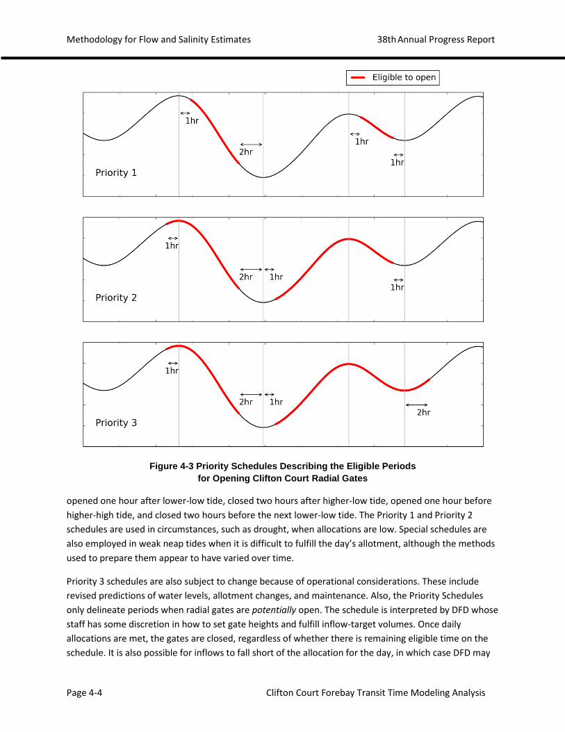
Radial gate flows are manipulated to satisfy multiple objectives. Operators seek to reduce the effect of Clifton Court operations on south Delta water levels, meet SWP allocations from the Delta, and limit entrainment of federal Endangered Species Act- and California Endangered Species Act- protected species. Preliminary gate schedules are developed in advance by the DWR Operation and Maintenance Division (DWR O&M) based on tide tables. These requests specify when the gates are eligible to be open according to the Priority System, which is a set of tidal rules developed to reduce impacts on south Delta diverters. The most common schedule is the one labeled as Priority 3 in Figure 4-3. The gates may be



Figure 4-3 Priority Schedules Describing the Eligible Periods for Opening Clifton Court Radial Gates

opened one hour after lower-low tide, closed two hours after higher-low tide, opened one hour before higher-high tide, and closed two hours before the next lower-low tide. The Priority 1 and Priority 2 schedules are used in circumstances, such as drought, when allocations are low. Special schedules are also employed in weak neap tides when it is difficult to fulfill the day’s allotment, although the methods used to prepare them appear to have varied over time.

Priority 3 schedules are also subject to change because of operational considerations. These include revised predictions of water levels, allotment changes, and maintenance. Also, the Priority Schedules only delineate periods when radial gates are potentially open. The schedule is interpreted by DFD whose staff has some discretion in how to set gate heights and fulfill inflow-target volumes. Once daily allocations are met, the gates are closed, regardless of whether there is remaining eligible time on the schedule. It is also possible for inflows to fall short of the allocation for the day, in which case DFD may



change gate heights or the Joint Operations Center may reschedule gate openings to make up for unused allocation on the following day.

The Clifton Court radial gates can be operated close to being fully open, which means approximately 15–18 ft above the sill, or be partially opened to as little as a few feet above the sill. Operating with the radial gates fully open was apparently a more prevalent operation early in the history of the Forebay, although data from the last 10 years suggest this type of operation is still used with some frequency when water supply demands are adequate, and fish triggers do not constrain operations. In recent years, a sipping strategy has been adopted, in which the radial gates are opened to a much smaller height for a longer period, attempting to take in water over the full eligible opening period at a lower rate. Sipping is the predominant gate operation in recent years during the January–June period of greatest fishery concern.

Across the Forebay from the radial gates, water flows out an intake canal to the Banks Pumping Plant. Banks Pumping Plant has a capacity of 10,300 cfs and lifts water 244 ft from the Delta to the California Aqueduct. The daily export volume is dictated by project demands, agreements, and regulatory constraints; but the hour-by-hour scheduling of pumping is planned around available water in the Forebay, the price of electricity, and maintenance of the facilities.

As a guiding goal, DFD likes to leave water levels at approximately 1.8 ft NAVD88 (-0.5 ft NGVD29) at midnight. This rule is apparently adjusted for challenging tidal circumstances or large-flow allocations. The balance between exports and gate allocations is achievable on a daily average basis during spring tides, but this is more difficult to achieve during neap tides when the head difference across the gates is small.

The main fish protection facilities are in the intake channel. Before water is pumped, it traverses the John E. Skinner Delta Fish Protective Facility (SDFPF) (Figure 4-4). The SDFPF was designed to protect fish from entrainment into the California Aqueduct by diverting them into holding tanks where they can be salvaged and safely returned to the western Delta. Water is drawn to the SDFPF from the Forebay via the intake canal and past a floating trash boom. The trash boom is designed to intercept floating debris and guide it to a trash conveyor on shore. Water and fish then flow through a trash rack, which is equipped with a trash rake, to a series of louvers arranged in a V pattern shown in Figure 4-4. Fish are behaviorally guided via the louvers and directed to holding tanks for salvage. More complete descriptions of the facility, its efficiency, and sampling challenges can be found in Castillo et al. (2012). Details of the facility are not included in our model domain, which terminates at the trash rack.

Byron Bethany Irrigation District (BBID) diverts a small additional volume from a location along the SWP intake downstream of the fish protection facilities at 37° 48’ 51.81” north latitude and 121° 36’ 20.71” west longitude. Operators also strive to prevent water levels in the Forebay from dropping below approximately 0.3 ft NAVD88 (-2.0 ft NGVD29) because of potential cavitation issues at the BBID’s diversion point. Low water levels also can potentially limit conveyance in the main Forebay during high-flow or low-exterior water levels. Such conditions were not the focus of our study, but the presented dredging operations would be expected to benefit conveyance capacity through Clifton Court.



Figure 4-4 Skinner Delta Fish Protection Facility



4.2 Model Description

4.2.1 Hydrodynamics

The model used for this analysis is the 3D SCHISM (Zhang and Baptista 2008; Zhang et al. 2015; 2016). Although this is the same computational code used in the Bay-Delta SCHISM project (Ateljevich et al. 2013), the domain in this case is restricted to the Forebay intake channel up to the SDFPF trash rack.

As used here, SCHISM solves the 3D hydrostatic Reynolds-averaged shallow water equations, including mass conservation and horizontal momentum conservation. For this project, we have dropped terms involving baroclinic pressure (salt and temperature gradients are small). Density terms in the turbulence closure were also neglected. We experimented with horizontal viscosity, although the results here are presented without it, which is the most common practice among 3D models in the estuary. The elimination of horizontal viscosity is justified on the assumption that a well-resolved horizontal grid and modest amount of numerical diffusion are sufficient to model horizontal mixing.

Boundary conditions for the water column are given by wind stresses at the free surface and shear at the bed. For wind, the boundary condition is

ν𝜕𝜕𝜕𝜕𝜕𝜕𝜕𝜕

= 𝜏𝜏𝑤𝑤 , at 𝜕𝜕 = 𝜂𝜂

(1)

using the wind stress (𝜏𝜏𝑤𝑤) formulation from Pond and Pickard (1983). The boundary condition at the bed (𝜕𝜕 = −ℎ) is

ν𝜕𝜕𝜕𝜕𝜕𝜕𝜕𝜕

= 𝜏𝜏𝑏𝑏 , at 𝜕𝜕 = −ℎ

(2)

with bottom stress (𝜏𝜏𝑏𝑏) derived from a quadratic formulation based on the velocity (𝒖𝒖𝑏𝑏) evaluated at the top of the bottom computational cell and is

𝜏𝜏𝑏𝑏 = 𝐶𝐶𝐷𝐷|𝒖𝒖𝑏𝑏|𝒖𝒖𝑏𝑏 (3)

The drag coefficient (𝐶𝐶𝐷𝐷) of roughness is calculated dynamically from a roughness parameter (z0=0.8 millimeters) by using standard boundary layer assumptions as described in Zhang and Baptista (2008).

The turbulent eddy viscosity (ν) is generated by using an independent set of turbulence closure equations, specifically the k-ε 2.5 equation closure with a background eddy viscosity of 0.0096 ft2s-1. As described previously, only terms related to barotropic characteristics of the mean flow were included in the closure calculations, such as production of turbulence by shear. We dropped terms associated with density stratification that play little role in Clifton Court dynamics. The closure is implemented in SCHISM using the Generic Length Scale approach of Umlauf and Burchard (2003). Relative to turbulence, the closure used in the stratified part of the Bay-Delta estuary (k-ω, for instance), the choice of the k-ε closure and the use of non-trivial background viscosity can be regarded as diffusive choices. Our parameter choices are intended to dissipate eddies that form during abrupt gate openings and propagate forth in the upper water column. The results seem to tally well with the 2008–2009 field



measurements, which were mostly taken during periods of light or medium wind. In windy conditions, pronounced layered flow does develop in both the model and field data.

4.2.2 Radial Gate Parameterization

We included the Forebay radial gates directly within the model, which is the domain that extends upstream of the gates to the junction with West Canal. This approach is somewhat more complex than just terminating the domain at the gates and imposing a flow. For our work, the approach has two compensating advantages. First, it is more extensible should the model need to be nested within the greater Bay-Delta. Second, the approach has a stabilizing effect on water levels during longer simulations in the presence of episodic data discrepancies between inflows and outflows.

No matter how the boundary on the gate side is approached, a reasonable rating formula is required to produce flows from water levels and radial gate heights. Daily average flows are inverted from Banks Pumping Plant tallies and midnight storage changes, but these are too coarse in time to use in a study of velocity. Finer time-step gate-flow estimates are also calculated by DWR, based on the antiquated Hills Equation. These take gate heights, interior, and exterior water levels as inputs, which are available at finer time scales, particularly after 2012. For this study, we incorporated the rating equation for the gates developed by Ateljevich et al. (2015). Further details may be found in that work or the Report. As a consequence of our approach, some of our gate flows in this chapter have considerably higher peak values than those plotted by MacWilliams and Gross (2013). In fact, our estimates are similar in magnitude to those of the most accurate methods reported in that work, called the “scaled gate equation.” But the authors used a different technique for the bulk of their analysis, disaggregating daily volume over the gate opening period with a flat line. This simplification results in peak flows, as much as 50 percent lower. One other notable thing about the MacWilliams and Gross (2013) approach is that the scaling they apply algebraically constrains water levels to match historical water-level changes on a daily basis. This is an advantage in historical modeling, as far as water levels are concerned, but it is harder to extend to hypothetical operations, such as our brief gate-export lagging experiment in section 4.5.4, “Transit Time.”

4.2.2.1 Evaporation

We did not include evaporation. Assuming a typical Central Valley summer evaporation rate of 0.75 ft/month, we expected evaporation in the Forebay to reach 20 cfs during July–August, but to be as low as 3–4 cfs during January–March when fishery concerns are highest. Either rate is small compared with other boundary uncertainties. Also, evaporation occurs diffusely over the whole surface and consequently has a particularly small effect on momentum and currents.

4.2.3 Particle Tracking

We modeled transit by using streamlines of neutrally buoyant particles introduced randomly in the top 3.3 ft (1 meter [m]) of the water column within the wingwalls downstream of the radial gates. For purposes of this study, the equations of motion for each particle are accordingly advection with flow.



𝑑𝑑𝒙𝒙𝒊𝒊𝑑𝑑𝑑𝑑

= 𝒖𝒖(𝒙𝒙𝒊𝒊, 𝑑𝑑) (4)

where 𝒙𝒙𝒊𝒊 is the position of the i’th particle. This formulation omits the random-walk component because of eddy diffusivity that provides a linkage with the transport equation for dissolved species. Particles are injected randomly in the upper part of the water column, but afterwards vertical migration is slower than that of a particle subject to turbulent mixing. This amounts to an implicit stabilizing “behavior,” particularly in the vertical direction; particles do not jump vertically from one contrasting horizontal flow structure to another. This is more of an important assumption in windy flow, where the top and bottom of the water column can have very different velocity patterns. In flows driven by gates and exports, vertical structure in the flow is limited to mild shear and the impact of the assumption is smaller.

4.2.4 Mesh and Time Discretization

The horizontal mesh is shown in Figure 4-5. The mesh is mostly triangular, but contains quadratic elements near the radial gates and pump intakes. The mesh is unstructured, with flexible resolution to conform to terrain features. Overall, there are 25,716 horizontal elements in the model. Typical length scales are 5 m near the radial gates, 10 m near the pump intakes, and 20–30 m in the mid-Forebay.

The vertical mesh in the present model uses an S-grid (Song and Haidvogel 1994) with eight levels. An S-grid is a terrain-conforming vertical grid with linear (triangles) or bilinear (quadrilaterals) representation of bathymetric and spatial features. For most of the domain and under typical reservoir heights, these yield a vertical resolution of approximately 0.8 ft (0.25 m) in the body of the Forebay. In deeper regions, eight levels represents a vertical resolution of 3.3 ft (1 m) or coarser in places like the scour hole. In these less-resolved areas, the mesh is somewhat clustered near the surface, so that region remains relatively resolved.

The time step for the hydrodynamic model is 60 seconds, which we found was the coarsest time step that smoothly integrates transitions at abrupt gate openings without creating spurious currents. Hydrodynamic information for particle tracking is saved at intervals of 120s, or every other hydrodynamic time step. The particle tracking model reports at this nominal time step of 120s, but the integration scheme uses a subdivided time step, typically 12s.



Figure 4-5 Horizontal Mesh



4.3 Input Data Sources The major time-series data requirements for our model are Banks Pumping Plant pumping flows and Clifton Court radial gate heights and wind, all required at an hourly or better time step. Additionally, the model requires bathymetric elevations.

Below we list where we acquired data for the various years that we simulated and the reliability and caveats we believed to be associated with those sources. One that applies generally involves time stamps of historical data. DWR operational databases return data time stamped with Daylight Savings Time. We preferred to model in Pacific Standard Time and attempt to align data to Pacific Standard Time (PST), but have found in some cases there are ambiguities that arise over the shifting of older records. Similar comments apply to other sources of data, with California Data Exchange Center (CDEC) serving data with time stamps that are not rigorous. The DWR NCRO and U.S. Geological Survey (USGS) distribute data time stamped in PST.

4.3.1 Banks Pumping Plant Flow

Instantaneous flow at the pumps is not observed directly. This is a matter of some confusion and lore. Flow measurement equipment has been installed in the past, but the instruments have not been maintained. Instead, DFD infers instantaneous flows by logging which pumping units are operating and summing their individually rated capacities. The start- and stop-times upon which flow estimates are made have been stored with very fine temporal resolution as part of the internal DWR Systems Applications and Products (SAP) data logging system since 2006 (SAP report titled Unit Status Log Exclude Report 2). Earlier historical records are available from the Interagency Ecological Program and other sources, but these were not utilized in this study. Daily averaged exports constructed from spreadsheets using similar methods and formulas are reported in public databases, such as CDEC. BBID diversions are taken from the CDEC station BBI, which is a daily average. As the total volume is low, no site-specific processing is performed on this data.

4.3.2 Radial Gate Operations

We modeled the Clifton Court radial gates explicitly by using a radial gate-rating formula. This calculation requires gate heights, interior water levels, and exterior water levels. Interior water levels are taken from the hydrodynamic model’s dynamic state. Radial gate heights and exterior gage heights must be supplied as input data.

Historical gate heights, going back to approximately 2011, are available from the DWR Control Systems Branch (CSB) Information Server at a very high time resolution (< = 10 min), which captures the gradual opening and closing of the gate.

For exterior water levels, we used historical gauge heights from the DWR NCRO station Old River at Clifton Court Ferry (B95340). These differ slightly from the upstream water levels recorded by DWR O&M. We chose the NCRO station because we felt more confident about the datum.



4.3.3 Bathymetry

The main bathymetry survey used in the study was done in January, 2016 by NCRO in connection with this project. The survey is multi-beam and very dense around the scour hole, but single beam with adaptive resolution in the sediment and finger areas beyond, where the shallows make multi-beam collection less practical because it has limited extent at close range. At times, we will discuss an earlier collection in 2004 also conducted by NCRO using single-beam soundings. This collection was less resolved in the scour-hole area, because it has no multi-beam component. Farther afield in the sediment deposition area, it followed a more gridded sampling approach, which is less adaptive to bathymetric features but is generally more resolved.

The two collections reveal different morphological states of the Forebay, particularly in the scour and depositional areas near the gate. In 2004, the scour hole was shallower and channelization through the perimeter sediment ring was less developed. By 2016, the scour hole had deepened and a prominent subchannel through the sediment had developed in the north. Neither survey is detailed enough to make detailed quantitative comparisons.

4.3.4 Wind

In this modeling application, we made the simplification that wind is uniform over the full domain. Because of data gaps, we made use of three local stations: Clifton Court Gates (CDEC code CLC), Banks Pumping Plant (CDEC code HBP), and Rough and Ready Island (CDEC code RRI) near Stockton. The CLC station is the only one of these stations situated within the modeling domain, and we attempted to make it our standard. But, CLC and HBP were new and only beginning to be archived during the 2008–2009 validation period, with regular CDEC coverage beginning respectively in July, 2008 and October, 2009. The authors received an unarchived copy of wind data from MacWilliams (pers, comm, Jul 13, 2016) that extends the Clifton Court Radial Gate wind record to most of summer 2008 that appears to originate from data loggers at CLC.

CLC was also subject to erratic values in January, 2017 during our very-high-flow particle analysis. Specific details about imputing missing data are available in Shu and Ateljevich (2017). We found the wind field to be complex, taking on directionally and seasonally mixed characteristics of wind at HBP and RRI.



4.4 Calibration and Validation In this section, we compare model results to observed data, including Forebay water levels, gate flow, vertical velocity, and drifter tracks. The comparison is mostly a calibration result, rather than validation, because we had access to the data during model development, and the study used model comparisons to make a small number of parameter and algorithmic choices (roughness, background eddy viscosity and turbulence closure). We utilized several data sources. Significantly, in 2008–2009, the USGS conducted a series of field studies in the Forebay, including drifter releases in June, 2008, and velocity measurements, by using upward-looking ADCPs between September, 2008, and January, 2009. We also validated flow in the intake channel against USGS transects. For brevity, only the velocity component is described here. Water level validation, intake flows and particle trajectories may all be found in the Report. The water levels and intake flows corroborate the gate rating of Ateljevich (2015).

Between fall 2008 and spring 2009, the USGS established upward-looking ADCPs at the locations noted in Figure 4-6. The instruments were deployed during two periods — the first period was 09/19/2008–01/13/2009 and the second period was 01/13/2009–04/14/2009. The configuration of the instruments and data within the water column is sketched in Figure 4-7. Each ADCP is anchored to the bed, with the observation cones extending upward. Velocities cannot be observed over a blanking distance of 1.65 ft (0.50 m). Above that, the observations were arranged in one, two, or three 1.65 ft (0.50 m) cells, allowing a limited glimpse of vertical velocity structure. The region immediately below the surface is not normally reported because of errors caused by reflection and sidelobe interference and, given the shallowness of the Forebay, only one station had more than two good bins. In the field data, velocities are averaged over the vertical cell extents. In the model, which is smoother in velocity, we extracted cell mid-points.

Figure 4-8–Figure 4-13 show modeled compared with observed results at the six locations for both components of velocity. The plots are marked with the direction (u is eastward, v is northward) as well as an ADCP bin (1 or 2). Only two bins were used per station, and just one was used in CCFCN.

The model reproduces the full range of velocities near the pumps (station CCFWE). It also performs well on velocities midway between the gates and pumps, particularly at station CCFSC. On the eastern edge of the Forebay (CCFNE), the most significant velocities are also captured well, although there are stations (e.g., CCFNO) where velocities are seemingly small compared with background fluctuations.

The two largest discrepancies involve the upper velocity bins at stations CCFSC and CCFCN, and in each of these cases, only one component of velocity and one bin are affected. In the case of CCFSC, large easing (u) velocities are present in the upper bin of the observations, but are not in the model. At station CCFCN, large northing (v) velocities develop in the upper bin of the model, but not in the observations. In both cases, the issue is a far-field effect of gate or pumping operations (wind is weak) and in both locations bathymetry is part of the issue. Swapping 2004 bathymetry for 2016 bathymetry does not fix the problem completely, but it does change the component of velocity that is problematic.



Figure 4-6 U.S. Geological Survey Sampling Locations for Upward-looking ADCPs and Drifters

Notes: ADCP = acoustic Doppler current profiler, CCFCN, CCFNE, CCFCS, and CCFWE = USGS codes for ADCP locations in Clifton Court Forebay, A, B = drifter release points.

Figure 4-7 Sketch of Upward-Looking ADCP Beam and Sampling Bins

Notes: ADCP = acoustic Doppler current profiler, ft = feet, m = meter



Figure 4-8 Boundary Flows and Wind (top) and Comparisons with Observed Velocity at Site CCFWE

Notes: ADCP = acoustic Doppler current profiler, cfs = cubic feet per second, ft/s = feet per second, CCFWE = USGS code name for location in Clifton Court Forebay, mph = miles per hour The U (easting) and V (northing) part of the axis label indicate direction, and the V1 and U1 (lower charts) and V2 and U2 (mid and upper charts) indicate the vertical position of the ADCP bin.



Figure 4-9 Boundary Flows and Wind (top) and Comparisons with Observed Velocity at Site CCFNE

Notes: ADCP = acoustic Doppler current profiler, CCFNE = USGS code for station in Clifton Court Forebay, cfs = cubic feet per second, ft/s = feet per second, mph = miles per hour



Figure 4-10 Boundary Flows and Wind (top) and Comparisons

with Observed Velocity at Site CCFSC

Notes: ADCP = acoustic Doppler current profiler, CCFSC = USGS code for a station in Clifton Court Forebay, cfs = cubic feet per second, ft/s = feet per second, mph = miles per hour The u (easting) and V (northing) part of the axis label indicate direction and the V1 and U1 (lower charts) and V2 and U2 (mid and upper charts) indicate the vertical position of the ADCP bin.



Figure 4-11 Boundary Flows and Wind (top) and Comparisons with Observed Velocity at Site CCFCS

Notes: ADCP = acoustic Doppler current profiler, CCFSC = USGS code for a station in Clifton Court Forebay, cfs = cubic feet per second, ft/s = feet per second, mph = miles per hour The u (easting) and V (northing) part of the axis label indicate direction and the the V1 and U1 (lower charts) and V2 and U2 (mid and upper charts) indicate the vertical position of the ADCP bin.




with Observed Velocity at Site CCFNO

Notes: ADCP = acoustic Doppler current profiler, CCFNO = USGS code for a station in Clifton Court Forebay, cfs = cubic feet per second, ft/s = feet per second, mph = miles per hour The u (easting) and V (northing) part of the axis label indicate direction and the V1 and U1 (lower charts) and V2 and U2 (mid and upper charts) indicate the vertical position of the ADCP bin.




with Observed Velocity at site CCFCN

Notes: ADCP = acoustic Doppler current profiler, CCFCN = USGS code for a station in Clifton Court Forebay, cfs = cubic feet per second, ft/s = feet per second, mph = miles per hour The u (easting) and V (northing) part of the axis label indicate direction and the V1 and U1 (lower charts) and V2 and U2 (mid and upper charts) indicate the vertical position of the ADCP bin — in this case there is only one bin.



4.5 Transit Time and Velocity Analysis

4.5.1 Dredge and Fill Alternatives

We experimented with a number of dredging and filling alternatives to examine their effect on transit time. The alternatives are permutations of the following components, many of which are illustrated in Figure 4-14.

Base. The base is established by the 2016 bathymetry survey.

Fill scour hole. This option involves filling the scour hole immediately beyond the radial gates to -4 ft (-1.22 m) NAVD88 or -6.56 ft (-2. m) NAVD88 in combination with certain dredging options, as described below. In 2016, the scour hole was surveyed as being 63 ft deep. Filling the scour hole was deemed beneficial for predator habitat reduction, and we included filling the scour hole for any dredging option marked “filled.”

Fill finger channel. This option involves filling the northern subchannel through the sediment ring to 0.656 ft (-0.2 m) NAVD88. There were two motives for filling this channel. First, it reinforces a more northward velocity path that sends particles to the northwest side of the Forebay where they tend to linger. Second, the feature resembles dredging, and we preferred to focus on other dredging alternatives in isolation. The finger channel is filled for any option marked “filled,” except for the curved dredge and near gate dredge, which overlap and effectively overwrite the bathymetry of the finger channel.

Dredge straight channel. This option involves dredging a straight path from the gates to the pumps at -6.56 ft NAVD88. Two variants were attempted, one 325 ft (100 m) wide and the other 1,000 ft (300 m) wide. Scour hole is filled to -6.56 ft NAVD88 for options marked “filled.”

Dredge curved channel. This option dredges an arc path from the gates to the pumps. The pattern was inspired by streamlines in moderate flow. Although this option seemed promising in early work over a limited set of operations and winds, ultimately it turned out to yield fewer benefits.

Dredge sediment near gate. In this option, the sediment ring near the gate is dredged to -4 ft NAVD88. The scour hole is also filled to -4 ft NAVD88, if marked “filled.”

Dredge southern sediment near gate. The southern half of the sediment ring near the gate is dredged to -4 ft NAVD88. The scour hole is filled to -4 ft NAVD88 for options marked “filled. The quantity of materials moved for this option is lower than those moved for the 1,000 ft-wide straight channel.

4.5.2 Methods

For the analysis of bathymetry changes, we compared the distributions of transit times resulting from particle releases over a variety of operational and tidal conditions. After developing flow fields for each weeks, we made two releases of 7,500 particles, each for a duration of approximately two weeks. The first began April 26, 2016, and represented a period of low-medium-gate/pumping flows (1,175 cfs daily



Figure 4-14 Base Case and Dredging and Filling Options Explored in This Report

Notes: Elev. = elevation, ft NAVD88 = feet in North American Vertical Datum of 1988



Figure 4-15 Radial Gate Flow, Banks Intake Flow, and Wind Conditions for 2012 (top), 2016 (middle), and 2017 (bottom)

Notes: Banks = Harvey O. Bank Pumping Plant, cfs = cubic feet per second, mph = miles per hour

average exports) and moderate wind. The second began December 31, 2011, and represented a period of relatively high-gate/pumping flows (3,800 cfs of exports). We also present a few results for January 13, 2007 under flood conditions (9,700 cfs of exports), which are interesting as a bracketing case, but are seldom relevant for the traditional January–June fish protection season. Banks Pumping Plant pumping, gate flows and wind conditions for these periods are shown in Figure 4-15. Note that as flows get larger, Banks Pumping Plant pumping transitions from a pulse flow pattern (based on electricity prices) to a constant flow (based more on maintenance considerations).



During each of the release periods, particles were introduced randomly using a distribution proportional to flow. Spatially, each particle released was random (uniform) and was situated between the wingwalls’ interior of the radial gate. After introduction, particles were observed until 14 days after the introduction of the last particle, for a total of 28 days of simulation. We recorded particle paths, velocity results, as well as summaries of entry and exit details for each particle. Particle trajectories were scrutinized for all the bathymetry and flow options. A selection of trajectories is plotted in section 4.5.3.1, “Patterns and Variations in Particle Trajectories” and is paired with velocity gradient spatial plots to give a sense of the manner and extent to which dredging and filling can manipulate particle streamlines.

4.5.3 Key Results

4.5.3.1 Patterns and Variations in Particle Trajectories

The Forebay experiences several flow patterns depending on operations at the gates, export pumping, and wind. Generally speaking, the stronger the forcing by flow, the simpler the current structure is and the more bendable the main trajectories are under dredging alternatives. Figure 4-16 shows particle paths and velocity gradients resulting from inflow on April 27, 2016 for the base case, which is a case where the scour and finger hole are filled, and a case with these fill actions plus the 1,000 ft straight dredging alternative. Panes (a), (c), and (e) show particle trajectories and panels (b), (d), and (f) show the respective velocity gradients.

The filling option accelerates particles through the scour region, causing particle trajectories that move far over the gate opening, but also mix more vigorously. It also slightly accentuates a tunnel-like path through the scour and deposition that may be exploitable by predators. The option that adds a straight channel not only accelerates the particles, but bends streamlines more towards the gate. This option reduces transit time mostly in low flows, but it also produces the strongest velocity gradients.

Figure 4-17 shows analogous trajectories and gradients in the 2012 high-flow case. In this case, many of the particles traverse the Forebay within a day of when they enter the gates. Others make it most of the way, leaving them clustered within the zone of influence of the pumps the next day. The 1,000 ft (300 m) dredge reduces transit time initially, conspicuously guiding particles towards the pumps.

Figure 4-16 and Figure 4-17 are representative of the trends, but streamlines vary considerably based on recent flow and wind conditions, particularly at the beginning and ending of a gate operation, when particles can take routes that are much less direct. Particles that do not make it to exports when a day’s operations conclude are subject to chaotic mixing by eddies or wind that persist through inertia. Even in light wind, particles do not remain clustered for long. If they are retained in the Forebay for longer than approximately the mean residence time (or approximately four days, whichever is shorter) they will start to become randomly distributed.



Figure 4-16 Particle Trajectories and Velocity Gradients in Low Flow

Under Three Bathymetry Options

Notes: (a) = particle trajectory for the base bathymetry under a 2016 low-flow allotment, (b) = maximum velocity gradient over the same gate opening as in (a) for base bathymetry, (c-d) = particle trajectories and velocity gradients with scour hole and finger hole filled, (e-f) = particle trajectories and velocity gradients for case with these fill actions plus a 1,000 ft (300 m) -wide straight channel from gates to export intake



Figure 4-17 Particle Trajectories and Velocity Gradients in High Flow

Under Three Bathymetry Options

Notes: (a) = particle trajectory for the base bathymetry under a 2012 high-flow allotment, (b) = maximum velocity gradient during the same gate opening as (a) for base bathymetry, (c-d) = particle trajectories and velocity gradients with scour hole and finger hole filled, (e-f) = particle trajectories and velocity gradients for case with these fill actions plus a 1,000 ft (300 m)-wide straight channel from gates to export intake



4.5.4 Transit Time

The transit time of particles from Clifton Court gates to the Banks Pumping Plant intake can be summarized in retention curves that are the analog of Kaplan-Meier survival plots. Figure 4-18 shows plots of retention curves for the base case and filling options for the 2016 low-flow case. Filling the scour hole leads to improve transit time, in particular early transit, and filling the finger channel has an insignificant effect. The 2012 high-flow case is omitted here, but is included in the Report. The larger flow makes a big difference in reducing transit time relative to bathymetry. The gains by filling the scour hole are modest, because the extra velocity that helps usher particles across the scour region also generates chaotic mixing as shown in the particle trajectory images from Figure 4-16 and Figure 4-17. Filling the scour hole is an important option, even with modest gains, for two reasons. First, it is motivated by other goals, such as reduction of predator habitat, in which case we only have to establish lack of harm in terms of transit time. Second, the option is compatible with or even synergistic with dredging options.

Retention curves for the options including dredging are shown in Figure 4-19 and Figure 4-20 . When combined with filling of the scour hole and finger channel, the 1000 ft straight channel and full dredging of the sediment ring both achieve a substantial reduction in transit time in the 2016 low flow case relative to filling alone. The other projects do not achieve big marginal benefits compared to filling. In the 2012 high flow case, all the dredging options increased transit within the first two days. After two days, there are few particles left in the system, so results are probably less reliable – assuming the results are still valid, they indicate a slight worsening of transit time.

Flow plays a deciding role in transit time under any bathymetry option. To underscore this point, Figure 4-21 compares retention time with the base bathymetry among three years with very different flows: 2016 (daily average exports 1,175 cfs), 2012 (3,800 cfs), and 2017 (9,700 cfs). Gate flows are generally similar on a daily averaged basis. The mean volumetric residence time of these samples ranges from more than seven days in 2016 to less than one day in 2017. Cross-hatching in the 2017 plot indicates estimates that are influenced by censorship; particles in 2017 exit the system early and sample sizes going out 10 days or so are very small. Such cross-hatching would appear in the other plots as well, but the censorship starts more than 14 days into the experiment and is caused by the termination of particle tracking. The dominance of flow holds for any bathymetry option.

With flow being so important to transit, it seems natural to ask whether relative timing of gate and export flows is equally important. We examine this but concluded that shifts in relative timing were not very important.



Figure 4-18 Retention Curves for Base and Filling Options, Low-Flow (2016) Case

Figure 4-19 Retention Curves for Base and Dredge + Fill Options, Low-Flow (2016) Case



Figure 4-20 Retention Curves for Base and Dredge + Fill Options, High-Flow (2012) Case

Figure 4-21 Retention Curves for Base Bathymetry in Low-medium Flow (2016), Medium-High Flow (2012), and Extreme High Flow (2017)

Note: Cross-hatching indicates points that are developed with censored data.



4.6 Discussion In this study, we developed a transit time model of the Forebay and validated the model in terms of observed water levels, velocities, and particle trajectories. The model successfully reproduces observed velocities at a number of stations in the Forebay, particularly those that are forced by gate and pumping operations. Our velocity results in high wind are consistent with prior modeling, but there is limited field data to corroborate the complex exchange flows that develop under these conditions.

Our particle tracking results suggest that trajectories are influenced in a predictable way by gate and pump flows, with higher flows leading to faster transit. These boundary flows move particles across the Forebay in a velocity pattern with a simple vertical structure. Eddies and wind-generated velocities create more complex velocities that disperse the particles. It is likely that the most effective methods for reducing transit time will be those that focus on primary flows and coax particles across the Forebay soon after entry. These are the actions that produce velocities that are large enough to remain relevant after biological behavior is factored in. They are also the most dependable to model.

By far, the most important variables determining transit time under Reynolds-averaged flow are gate and export flows, which tend to vary together on a daily averaged basis under current policy. When gate and export flows are low (1,175 cfs daily average), volumetric residence time is fairly long (eight days in our example), and only a modest fraction of particles entering the gates makes it across the Forebay to be salvaged within 72 hours. Particles advance in advective pulses as operations alternate on and off, and at lower flows it can take several days to cross the Forebay. At the same time, the particles are dispersed by secondary or wind-driven currents. In strong gate and pumping flows (4,000 cfs), volumetric residence time is short (two days), many particles are entrained within a day, and a majority of particles reach the pumps within 72 hours. Particles that are entrained are swept along by larger velocities, which may be important where biological behavior is involved. Particles that are not salvaged are dispersed chaotically by eddies into regions where entrainment rates are lower.

Of the bathymetry manipulations we tested, filling the scour hole seems like a promising step. This filling accomplishes some of what is possible in terms of transit time reduction. Filling the scour hole is associated with other biological and logistical advantages and is compatible with the various dredging options, enhancing their benefits. Possible disadvantages that might arise from this action are higher local velocities and more-pronounced velocity gradients. In a biological setting, alleys of high-velocity water might be attractive to predators, in which case the reduction in transit time would be offset by higher hazard rates. Additionally, of course, the sediment dynamics in this area are complex, and maintaining the scour hole in its filled state and a dredged channel in its deeper state would be an engineering challenge. The other filling option we looked at, filling the finger channel through the sediment ring beyond the scour hole, had only a minor effect.

Of the dredging options, the ones that seemed most beneficial were the 1,000 ft (300 m) wide dredged straight channel and the dredging of the sediment ring that lies beyond the scour hole. These options achieve a substantial improvement in early salvage relative to the base bathymetry, particularly in the low-flow 2016 hydrology. Both are large-scale proposals, and their scaled-down variants do not achieve nearly as much. Neither option is as effective if the scour hole is not filled. Also, in high flow, the straight



channel conspicuously prolongs transit time after about two days. This may not be important given that transit time is, in any event, still quite low.

In the Report, we comment on enhancements to the model and further study from the point of view of transit time and survival analysis.



4.7 References Cited

Ateljevich E, Nam K, Zhang Y, Wang R, Shu Q. 2014. “Bay-Delta SELFE calibration overview.” In: Methodology for Flow and Salinity Estimates in the Sacramento-San Joaquin Delta and Suisun Marsh. 35th Annual Progress Report to the State Water Resources Control Board. Chapter 7. Sacramento (CA): Bay-Delta Office. Delta Modeling Section. California Department of Water Resources.

Ateljevich E, Tu M-Y, Le, K. 2015. “Calculation Clifton Court Forebay inflow and re-rating the forebay gates.” In: Methodology for Flow and Salinity Estimates in the Sacramento-San Joaquin Delta and Suisun Marsh. 36th Annual Progress Report to the State Water Resources Control Board. Chapter 6. Sacramento (CA): Delta Modeling Section. California Department of Water Resources.

Castillo G, Morinaka J, Lindberg J, Fujimura R, Baskerville-Bridges B, Hobbs J, Tigan G, Ellison L. 2012. “Pre-screen loss and fish facility efficiency for delta smelt at the south Delta’s State Water Project, California.” San Francisco Estuary and Watershed Science. 10(4). Viewed online at: http://escholarship.org/uc/item/28m595k4. [Journal article].

Hills E. 1988. New Flow Equations for Clifton Court Gates. State Water Project Division of Operations and Maintenance. California Department of Water Resources. [Technical Memorandum].

MacWilliams ML and Gross E. 2013. “Hydrodynamic simulation of circulation and residence time in Clifton Court Forebay.” San Francisco Estuary and Watershed Science. 11(2). Viewed online at: http://escholarship.org/uc/item/4q82g2bz. [Journal article].

National Marine Fisheries Service. 2009. Final Biological Opinion and Conference Opinion of the Proposed Long-term Operations of the Central Valley Project and State Water Project. U.S. Department of Commerce. National Marine Fisheries Service. Viewed online at: http://www.westcoast.fisheries.noaa.gov/publications/Central_Valley/Water%20Operations/Operations,%20Criteria%20and%20Plan/nmfs_biological_and_conference_opinion_on_the_long-term_operations_of_the_cvp_and_swp.pdf. Accessed: June 4, 2009.

———. 2011. 2009 RPA with 2011 Amendments. U.S. Department of Commerce National Marine Fisheries Service. Viewed online at: http://www.westcoast.fisheries.noaa.gov/publications/Central_Valley/Water%20Operations/Operations,%20Criteria%20and%20Plan/040711_ocap_opinion_2011_amendments.pdf. Accessed: April 7, 2011.

Pond S and Pickard GL. 1983. Introductory Dynamical Oceanography. Second edition. Oxford (UK): Butterworth-Heinmann Ltd. 349 pp.

Shu Q and Ateljevich E. 2017 Clifton Court Forebay Transit Time Modeling Analysis. Sacramento (CA): Bay-Delta Office. Delta Modeling Section. California Department of Water Resources.

Song Y and Haidvogel DB. 1994. “A semi-implicit ocean circulation model using a generalized topography-following coordinate.” Journal of Computational Physics. 115(1). pp. 228-244. [Journal article].

http://escholarship.org/uc/item/28m595k4

http://escholarship.org/uc/item/4q82g2bz

http://www.westcoast.fisheries.noaa.gov/publications/Central_Valley/Water%20Operations/Operations,%20Criteria%20and%20Plan/nmfs_biological_and_conference_opinion_on_the_long-term_operations_of_the_cvp_and_swp.pdf





Umlauf L and Burchard H. 2003. “A generic length-scale equation for geophysical turbulence models.” Journal of Marine Research. 61(2)6. pp. 235–265.

Wilde J. 2006. “Priority 3 Clifton Court Forebay Operations for Extended Planning Studies.” In: Methodology for Flow and Salinity Estimates in the Sacramento-San Joaquin Delta and Suisun Marsh. 27th Annual Progress Report to the State Water Resources Control Board. Chapter 8. Sacramento (CA): Delta Modeling Section. California Department of Water Resources.

Zhang Y and Baptista AM. 2008. “SELFE: A semi-implicit Eulerian-Lagrangian finite-element model for cross-scale ocean circulation.” Ocean Modelling. 21(3-4). pp. 71-96. [Journal article].

Zhang Y, Ateljevich E, Yu HS, Wu CH, Yu J. 2015. “A new vertical coordinate system for a 3D unstructured-grid model.” Ocean Modelling. 85. pp. 16-31. [Journal article].

Zhang Y, Ye F, Stanev EV, Grashorn S. 2016. “Seamless cross-scale modeling with SCHISM. Ocean Modelling.” 102. pp. 64-81. [Journal article].

4.7.1 Personal Communications

MacWilliams ML, Partner at Anchor QEA, San Francisco (CA). Jul. 13, 2016 — email correspondence with Ateljevich, E, California Department of Water Resources Delta Modeling Section, Sacramento (CA) — transmitting wind data from prior Clifton Court study

38th annual progress report june 2017 chapter 4...

Documents