4824 ieee transactions on wireless communications,...

4824 IEEE TRANSACTIONS ON WIRELESS COMMUNICATIONS, VOL. 8, NO. 9, SEPTEMBER 2009

An Adaptive Geometry-Based Stochastic Model forNon-Isotropic MIMO Mobile-to-Mobile Channels

Xiang Cheng, Student Member, IEEE, Cheng-Xiang Wang, Senior Member, IEEE,David I. Laurenson, Member, IEEE, Sana Salous, Member, IEEE, and Athanasios V. Vasilakos, Member, IEEE

Abstract—In this paper, a generic and adaptive geometry-based stochastic model (GBSM) is proposed for non-isotropicmultiple-input multiple-output (MIMO) mobile-to-mobile (M2M)Ricean fading channels. The proposed model employs a combinedtwo-ring model and ellipse model, where the received signal isconstructed as a sum of the line-of-sight, single-, and double-bounced rays with different energies. This makes the modelsufficiently generic and adaptable to a variety of M2M scenarios(macro-, micro-, and pico-cells). More importantly, our model isthe first GBSM that has the ability to study the impact of thevehicular traffic density on channel characteristics. From the pro-posed model, the space-time-frequency correlation function andthe corresponding space-Doppler-frequency power spectral den-sity (PSD) of any two sub-channels are derived for a non-isotropicscattering environment. Based on the detailed investigation ofcorrelations and PSDs, some interesting observations and usefulconclusions are obtained. These observations and conclusions canbe considered as a guidance for setting important parametersof our model appropriately and building up more purposefulmeasurement campaigns in the future. Finally, close agreementis achieved between the theoretical results and measured data,demonstrating the utility of the proposed model.

Index Terms—Mobile-to-mobile channels, MIMO, non-isotropic scattering environments, space-time-frequency correla-tion function, space-Doppler-frequency power spectrum density.

I. INTRODUCTION

RECENTLY, mobile-to-mobile (M2M) communicationshave received much attention due to some new ap-

plications, such as wireless mobile ad hoc networks [1],relay-based cellular networks [2], and dedicated short rangecommunications (DSRC) for intelligent transportation systems

Manuscript received December 16, 2008; revised March 13, 2009 and May12, 2009; accepted May 12, 2009. The associate editor coordinating the reviewof this paper and approving it for publication was K. K. Wong.

X. Cheng and C.-X. Wang are with the Joint Research Institute forSignal and Image Processing, School of Engineering and Physical Sciences,Heriot-Watt University, Edinburgh EH14 4AS, UK (e-mail: {xc48, cheng-xiang.wang}@hw.ac.uk).

D. I. Laurenson is with the Joint Research Institute for Signal andImage Processing, School of Engineering and Electronics, The Universityof Edinburgh, Edinburgh EH9 3JL, UK (e-mail: [email protected]).

S. Salous is with the Center for Communication Systems, Schoolof Engineering, University of Durham, Durham DH1 3LE, UK (e-mail:[email protected]).

A. V. Vasilakos is with the Department of Computer and Telecommuni-cations Engineering, University of Western Macedonia, GR 50100 Kozani,Greece (e-mail: [email protected]).

X. Cheng, C.-X. Wang, and D. I. Laurenson acknowledge the supportfrom the Scottish Funding Council for the Joint Research Institute in Signaland Image Processing between the University of Edinburgh and Heriot-Watt University which is a part of the Edinburgh Research Partnership inEngineering and Mathematics (ERPem). This paper was presented in part atIEEE IWCMC’08, Crete, Greece, August 2008.

Digital Object Identifier 10.1109/TWC.2009.081560

(e.g., IEEE 802.11p standard) [3]. In contrast to conventionalfixed-to-mobile (F2M) cellular radio systems, in M2M systemsboth the transmitter (Tx) and receiver (Rx) are in motionand equipped with low elevation antennas. For M2M commu-nications, multiple-input multiple-output (MIMO) technologybecomes more attractive since multiple antenna elements canbe easily mounted on large vehicular surfaces. It is well-knownthat the design of a wireless system requires the detailedknowledge about the underlying propagation channel and acorresponding realistic channel model. Up to now, only fewmeasurement campaigns had been conducted to investigatesingle-input single-output (SISO) M2M channels [4]–[8], evenfewer to study MIMO M2M channels [9].

M2M channel models available in the literature can be cat-egorized as deterministic models [10] and stochastic models,while the latter can be further classified as non-geometricalstochastic models (NGSMs) (also known as parametric mod-els) [6] and geometry-based stochastic models (GBSMs) [11]–[14]. A deterministic M2M model based on the ray-tracingmethod was proposed in [10]. This model requires a detailedand time-consuming description of the propagation environ-ment and consequently cannot be easily generalized to a widerclass of scenarios.

A SISO NGSM proposed in [6] is the origin of the channelmodel standardized by IEEE 802.11p. This model determinesphysical parameters of a M2M channel in a completelystochastic manner by prescribing underlying probability distri-bution functions (PDFs) without presuming any underlying ge-ometry. Therefore, this model offers no conceptual frameworkto facilitate meaningful generalization into different scenarios.In addition, this pure parameter-based model needs to jointlyconsider many parameters for modeling MIMO channels,which leads to high complexity [15].

A GBSM is derived from the predefined stochastic distribu-tions of effective scatterers by applying the fundamental lawsof wave propagation. Such a model can be easily adapted todifferent scenarios by changing the shape of the scatteringregion (e.g., one-ring, two-ring, or ellipse). More importantly,the application of the concept of effective scatterers signifi-cantly reduces the complexity of a GBSM since only singleand/or double scattering effects need to be simulated [15].Moreover, for modeling MIMO channels, a GBSM can avoidthe inherent complexity problem of a NGSM as shown in [15].In [11] and [12], the first GBSM was proposed for isotropicSISO M2M Rayleigh fading channels and corresponding sta-tistical properties were investigated. In [13], a two-ring GBSMconsidering only double-bounced rays was presented for non-

1536-1276/09$25.00 c⃝ 2009 IEEE

Authorized licensed use limited to: Heriot-Watt University. Downloaded on November 12, 2009 at 09:48 from IEEE Xplore. Restrictions apply.

CHENG et al.: AN ADAPTIVE GEOMETRY-BASED STOCHASTIC MODEL FOR NON-ISOTROPIC MIMO MOBILE-TO-MOBILE CHANNELS 4825

isotropic MIMO M2M Rayleigh fading channels in macro-cellscenarios. In [14], the authors proposed a general two-ringGBSM with both single- and double-bounced rays for non-isotropic MIMO M2M Ricean channels in both macro- andmicro-cell scenarios.

None of the above GBSMs is sufficiently general to char-acterize a wide variety of M2M scenarios, especially for pico-cell scenarios, which have recently been considered by somemeasurement campaigns [4]–[9]. As demonstrated in [8], theimpact of the vehicular traffic density (VTD) on channelcharacteristics in micro- and pico-cell scenarios cannot beneglected, unlike in macro-cell scenarios. However, noneof the existing GBSMs has the ability to take this impactinto account. Although the Doppler power spectral density(PSD) is one of the most important statistics that significantlydistinguish M2M channels from F2M channels, more detailedinvestigations of the Doppler PSD in non-isotropic scatteringenvironments are surprisingly lacking in the open literature.Moreover, Doppler PSD characteristics for an ellipse M2Mchannel model are not yet known. Finally, frequency cor-relations of sub-channels with different carrier frequencies,studied in [16] for F2M channels, in M2M communicationshave not been studied so far, although orthogonal frequency-division multiplexing (OFDM) has already been suggested foruse in IEEE 802.11p.

Motivated by the above gaps, in this paper we propose a newGBSM that addresses all the aforementioned shortcomingsof the existing GBSMs. Based on the proposed model, thespace-time-frequency (STF) correlation function (CF) andthe corresponding space-Doppler-frequency (SDF) PSD arederived. The contributions and novelties of this paper aresummarized as follows.

1) We propose a generic GBSM for narrowband non-isotropic MIMO M2M Ricean fading channels. Theproposed model can be adapted to a wide variety ofscenarios, e.g., macro-, micro-, and pico-cell scenarios,by adjusting model parameters.

2) By distinguishing between the moving cars and thestationary roadside environments in micro- and pico-cellscenarios, our model is the first GBSM to consider theimpact of the VTD on M2M channel characteristics.

3) We propose a new general method to derive the exactrelationship between the angle of arrival (AoA) andangle of departure (AoD) for any known shapes of thescattering region, e.g., one-ring, two-ring, or ellipse, in awide variety of scenarios.

4) We point out that the widely used CF definition in[13], [14], [17], [18] is incorrect and is actually thecomplex conjugate of the correct CF definition as givenin Stochastic Processes [19].

5) From the proposed model, we derive the STF CF and thecorresponding SDF PSD, which are sufficiently generaland can be reduced to many existing CFs and PSDs,respectively, e.g., those in [11], [13], [14], [17], [18].In addition, our analysis shows that the space-DopplerPSD of a single-bounce two-ring model for non-isotropicMIMO M2M channels derived in [14] is incorrect.

6) Based on the derived STF CF and SDF PSD, we studyin more detail the degenerate CFs and PSDs in terms

of some important parameters and thus obtain someinteresting observations. Finally, the obtained theoreticalDoppler PSDs and measurement data in [6] are com-pared. Excellent agreement between them demonstratesthe utility of the proposed model.

The remainder of this paper is outlined as follows. SectionII describes the new adaptive GBSM for narrowband MIMOM2M Ricean fading channels. In Section III, based on theproposed new model, the STF CF and the corresponding SDFPSD are derived. Numerical results and analysis are presentedin Section IV. Finally, conclusions are drawn in Section V.

II. A NEW ADAPTIVE GBSM FOR NON-ISOTROPIC MIMOM2M RICEAN FADING CHANNELS

Let us now consider a narrowband single-user MIMO M2Mmulticarrier communication system with 𝑀𝑇 transmit and 𝑀𝑅

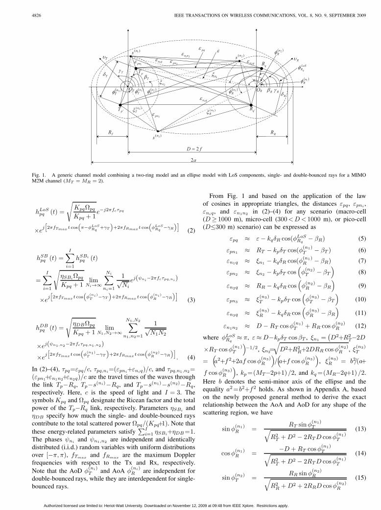
receive omnidirectional antenna elements. Both the Tx and Rxare equipped with low elevation antennas. Fig. 1 illustrates thegeometry of the proposed GBSM, which is the combinationof a single- and double-bounce two-ring model, a single-bounce ellipse model, and the LoS component. As an example,uniform linear antenna arrays with 𝑀𝑇 = 𝑀𝑅 = 2 wereused here. The two-ring model defines two rings of effectivescatterers, one around the Tx and the other around the Rx.Suppose there are 𝑁1 effective scatterers around the Tx lyingon a ring of radius 𝑅𝑇 and the 𝑛1th (𝑛1 = 1, ..., 𝑁1) effectivescatterer is denoted by 𝑠(𝑛1). Similarly, assume there are 𝑁2

effective scatterers around the Rx lying on a ring of radius 𝑅𝑅and the 𝑛2th (𝑛2 = 1, ..., 𝑁2) effective scatterer is denotedby 𝑠(𝑛2). For the ellipse model, 𝑁3 effective scatterers lieon an ellipse with the Tx and Rx located at the foci. Thesemi-major axis of the ellipse and the 𝑛3th (𝑛3 = 1, ..., 𝑁3)effective scatterer are denoted by 𝑎 and 𝑠(𝑛3), respectively.The distance between the Tx and Rx is 𝐷 = 2𝑓 with 𝑓denoting the half length of the distance between the two focalpoints of the ellipse. The antenna element spacings at theTx and Rx are designated by 𝛿𝑇 and 𝛿𝑅, respectively. It isnormally assumed that the radii𝑅𝑇 and 𝑅𝑅, and the differencebetween the semi-major axis 𝑎 and the parameter 𝑓 , are allmuch greater than the antenna element spacings 𝛿𝑇 and 𝛿𝑅,i.e., min{𝑅𝑇 , 𝑅𝑅, 𝑎− 𝑓} ≫ max{𝛿𝑇 , 𝛿𝑅}. The multi-elementantenna tilt angles are denoted by 𝛽𝑇 and 𝛽𝑅. The Tx and Rxmove with speeds 𝜐𝑇 and 𝜐𝑅 in directions determined by theangles of motion 𝛾𝑇 and 𝛾𝑅, respectively. The AoA of thewave traveling from an effective scatterer 𝑠(𝑛𝑖) (𝑖 ∈ {1, 2, 3})toward the Rx is denoted by 𝜙

(𝑛𝑖)𝑅 . The AoD of the wave

that impinges on the effective scatterer 𝑠(𝑛𝑖) is designated by𝜙(𝑛𝑖)𝑇 . Note that 𝜙𝐿𝑜𝑆𝑅𝑞

denotes the AoA of a LoS path.The MIMO fading channel can be described by a matrix

H (𝑡) = [ℎ𝑝𝑞 (𝑡)]𝑀𝑅×𝑀𝑇of size 𝑀𝑅 × 𝑀𝑇 . The received

complex fading envelope between the 𝑝th (𝑝 = 1, ...,𝑀𝑇 ) Txand the 𝑞th (𝑞 = 1, ...,𝑀𝑅) Rx at the carrier frequency 𝑓𝑐is a superposition of the LoS, single-, and double-bouncedcomponents, and can be expressed as

ℎ𝑝𝑞 (𝑡) = ℎ𝐿𝑜𝑆𝑝𝑞 (𝑡) + ℎ𝑆𝐵𝑝𝑞 (𝑡) + ℎ𝐷𝐵𝑝𝑞 (𝑡) (1)

where



1pn

)( 2ns)( 1ns

RT

)( 3ns

pT

pT

qR

qR

2pnqn1 qn2

1n

2n

3pn

qn3

)( 3nT )( 3n

R

21nn

fD 2

TR RR

1nT

2nT

3nT

1nR

2nR

3nR R

T

R

T

a2

T

RTO RO

LoSRq

pq

Fig. 1. A generic channel model combining a two-ring model and an ellipse model with LoS components, single- and double-bounced rays for a MIMOM2M channel (𝑀𝑇 = 𝑀𝑅 = 2).

ℎ𝐿𝑜𝑆𝑝𝑞 (𝑡) =

√𝐾𝑝𝑞Ω𝑝𝑞𝐾𝑝𝑞 + 1

𝑒−𝑗2𝜋𝑓𝑐𝜏𝑝𝑞

×𝑒𝑗[2𝜋𝑓𝑇𝑚𝑎𝑥 𝑡 cos

(𝜋−𝜙𝐿𝑜𝑆

𝑅𝑞+𝛾𝑇

)+2𝜋𝑓𝑅𝑚𝑎𝑥 𝑡 cos

(𝜙𝐿𝑜𝑆𝑅𝑞

−𝛾𝑅)]

(2)

ℎ𝑆𝐵𝑝𝑞 (𝑡) =

𝐼∑𝑖=1

ℎ𝑆𝐵𝑖𝑝𝑞 (𝑡)

=

𝐼∑𝑖=1

√𝜂𝑆𝐵𝑖Ω𝑝𝑞𝐾𝑝𝑞 + 1

lim𝑁𝑖→∞

𝑁𝑖∑𝑛𝑖=1

1√𝑁𝑖

𝑒𝑗(𝜓𝑛𝑖−2𝜋𝑓𝑐𝜏𝑝𝑞,𝑛𝑖)


(𝜙(𝑛𝑖)

𝑇 −𝛾𝑇)+2𝜋𝑓𝑅𝑚𝑎𝑥 𝑡 cos

(𝜙(𝑛𝑖)

𝑅 −𝛾𝑅)]

(3)

ℎ𝐷𝐵𝑝𝑞 (𝑡) =

√𝜂𝐷𝐵Ω𝑝𝑞𝐾𝑝𝑞 + 1

lim𝑁1,𝑁2→∞

𝑁1,𝑁2∑𝑛1,𝑛2=1

1√𝑁1𝑁2

×𝑒𝑗(𝜓𝑛1,𝑛2−2𝜋𝑓𝑐𝜏𝑝𝑞,𝑛1,𝑛2)


(𝜙(𝑛1)

𝑇 −𝛾𝑇)+2𝜋𝑓𝑅𝑚𝑎𝑥 𝑡 cos

(𝜙(𝑛2)

𝑅 −𝛾𝑅)]. (4)

In (2)–(4), 𝜏𝑝𝑞=𝜀𝑝𝑞/𝑐, 𝜏𝑝𝑞,𝑛𝑖=(𝜀𝑝𝑛𝑖+𝜀𝑛𝑖𝑞)/𝑐, and 𝜏𝑝𝑞,𝑛1,𝑛2=(𝜀𝑝𝑛1+𝜀𝑛1𝑛2+𝜀𝑛2𝑞)/𝑐 are the travel times of the waves throughthe link 𝑇𝑝−𝑅𝑞, 𝑇𝑝−𝑠(𝑛𝑖)−𝑅𝑞, and 𝑇𝑝−𝑠(𝑛1)−𝑠(𝑛2)−𝑅𝑞,respectively. Here, 𝑐 is the speed of light and 𝐼 = 3. Thesymbols 𝐾𝑝𝑞 and Ω𝑝𝑞 designate the Ricean factor and the totalpower of the 𝑇𝑝−𝑅𝑞 link, respectively. Parameters 𝜂𝑆𝐵𝑖 and𝜂𝐷𝐵 specify how much the single- and double-bounced rayscontribute to the total scattered power Ω𝑝𝑞/(𝐾𝑝𝑞+1). Note thatthese energy-related parameters satisfy

∑𝐼𝑖=1 𝜂𝑆𝐵𝑖+𝜂𝐷𝐵=1.

The phases 𝜓𝑛𝑖 and 𝜓𝑛1,𝑛2 are independent and identicallydistributed (i.i.d.) random variables with uniform distributionsover [−𝜋, 𝜋), 𝑓𝑇𝑚𝑎𝑥 and 𝑓𝑅𝑚𝑎𝑥 are the maximum Dopplerfrequencies with respect to the Tx and Rx, respectively.Note that the AoD 𝜙

(𝑛𝑖)𝑇 and AoA 𝜙

(𝑛𝑖)𝑅 are independent for

double-bounced rays, while they are interdependent for single-bounced rays.

From Fig. 1 and based on the application of the lawof cosines in appropriate triangles, the distances 𝜀𝑝𝑞 , 𝜀𝑝𝑛𝑖 ,𝜀𝑛𝑖𝑞 , and 𝜀𝑛1𝑛2 in (2)–(4) for any scenario (macro-cell(𝐷≥ 1000 m), micro-cell (300<𝐷< 1000 m), or pico-cell(𝐷≤300 m) scenario) can be expressed as

𝜀𝑝𝑞 ≈ 𝜀− 𝑘𝑞𝛿𝑅 cos(𝜙𝐿𝑜𝑆𝑅𝑞− 𝛽𝑅) (5)

𝜀𝑝𝑛1 ≈ 𝑅𝑇 − 𝑘𝑝𝛿𝑇 cos(𝜙(𝑛1)𝑇 − 𝛽𝑇 ) (6)

𝜀𝑛1𝑞 ≈ 𝜉𝑛1 − 𝑘𝑞𝛿𝑅 cos(𝜙(𝑛1)𝑅 − 𝛽𝑅) (7)

𝜀𝑝𝑛2 ≈ 𝜉𝑛2 − 𝑘𝑝𝛿𝑇 cos(𝜙(𝑛2)𝑇 − 𝛽𝑇

)(8)

𝜀𝑛2𝑞 ≈ 𝑅𝑅 − 𝑘𝑞𝛿𝑅 cos(𝜙(𝑛2)𝑅 − 𝛽𝑅

)(9)

𝜀𝑝𝑛3 ≈ 𝜉(𝑛3)𝑇 − 𝑘𝑝𝛿𝑇 cos

(𝜙(𝑛3)𝑇 − 𝛽𝑇

)(10)

𝜀𝑛3𝑞 ≈ 𝜉(𝑛3)𝑅 − 𝑘𝑞𝛿𝑅 cos

(𝜙(𝑛3)𝑅 − 𝛽𝑅

)(11)

𝜀𝑛1𝑛2 ≈ 𝐷 −𝑅𝑇 cos𝜙(𝑛1)𝑇 +𝑅𝑅 cos𝜙

(𝑛2)𝑅 (12)

where 𝜙𝐿𝑜𝑆𝑅𝑞≈ 𝜋, 𝜀≈𝐷−𝑘𝑝𝛿𝑇 cos𝛽𝑇 , 𝜉𝑛1 =

(𝐷2+𝑅2

𝑇−2𝐷×𝑅𝑇 cos𝜙

(𝑛1)𝑇

)−1/2, 𝜉𝑛2=

√𝐷2+𝑅2

𝑅+2𝐷𝑅𝑅 cos𝜙(𝑛2)𝑅 , 𝜉(𝑛3)

𝑇

=(𝑎2+𝑓2+2𝑎𝑓 cos𝜙

(𝑛3)𝑅

)/(𝑎+𝑓 cos𝜙

(𝑛3)𝑅

), 𝜉

(𝑛3)𝑅 = 𝑏2/(𝑎+

𝑓 cos𝜙(𝑛3)𝑅

), 𝑘𝑝=(𝑀𝑇−2𝑝+1)/2, and 𝑘𝑞=(𝑀𝑅−2𝑞+1)/2.

Here 𝑏 denotes the semi-minor axis of the ellipse and theequality 𝑎2=𝑏2+𝑓2 holds. As shown in Appendix A, basedon the newly proposed general method to derive the exactrelationship between the AoA and AoD for any shape of thescattering region, we have

sin𝜙(𝑛1)𝑅 =

𝑅𝑇 sin𝜙(𝑛1)𝑇√

𝑅2𝑇 +𝐷2 − 2𝑅𝑇𝐷 cos𝜙

(𝑛1)𝑇

(13)

cos𝜙(𝑛1)𝑅 =

−𝐷 +𝑅𝑇 cos𝜙(𝑛1)𝑇√

𝑅2𝑇 +𝐷2 − 2𝑅𝑇𝐷 cos𝜙

(𝑛1)𝑇

(14)

sin𝜙(𝑛2)𝑇 =

𝑅𝑅 sin𝜙(𝑛2)𝑅√

𝑅2𝑅 +𝐷2 + 2𝑅𝑅𝐷 cos𝜙

(𝑛2)𝑅

(15)



cos𝜙(𝑛2)𝑇 =

𝐷 +𝑅𝑅 cos𝜙(𝑛2)𝑅√

𝑅2𝑅 +𝐷2 + 2𝑅𝑅𝐷 cos𝜙

(𝑛2)𝑅

(16)

sin𝜙(𝑛3)𝑇 =

𝑏2 sin𝜙(𝑛3)𝑅

𝑎2 + 𝑓2 + 2𝑎𝑓 cos𝜙(𝑛3)𝑅

(17)

cos𝜙(𝑛3)𝑇 =

2𝑎𝑓 + (𝑎2 + 𝑓2) cos𝜙(𝑛3)𝑅

𝑎2 + 𝑓2 + 2𝑎𝑓 cos𝜙(𝑛3)𝑅

. (18)

Note that the above derived expressions in (5)–(18) are suffi-ciently general and suitable for various scenarios. For macro-and micro-cell scenarios, the assumption 𝐷≫max{𝑅𝑇 , 𝑅𝑅},which is invalid for pico-cell scenarios, is fulfilled. Then, thegeneral expressions of 𝜉𝑛1 and 𝜉𝑛2 can further reduce to thewidely used approximate expressions as 𝜉𝑛1≈𝐷−𝑅𝑇 cos𝜙

(𝑛1)𝑇

and 𝜉𝑛2 ≈ 𝐷+𝑅𝑅 cos𝜙(𝑛2)𝑅 , respectively. In addition, the

general expressions (13)–(16) for the two-ring model canfurther reduce to the widely used approximate expressionsas 𝜙

(𝑛1)𝑅 ≈ 𝜋−Δ𝑇 sin𝜙

(𝑛1)𝑇 and 𝜙

(𝑛2)𝑇 ≈ Δ𝑅 sin𝜙

(𝑛2)𝑅 with

Δ𝑇≈𝑅𝑇 /𝐷 and Δ𝑅≈𝑅𝑅/𝐷. Moreover, the relationships (17)and (18) for the ellipse model obtained by using our methodsignificantly simplify the relationships derived based on pureellipse properties, such as (A1)–(A3) in [20] and (27), (28),and (32) in [21].

Since the number of effective scatterers are assumed to beinfinite, i.e., 𝑁𝑖→∞, the proposed model in (1) is actually amathematical reference model and results in the Ricean PDF.Due to the infinite complexity, a reference model cannot beimplemented in practice. However, as mentioned in [22], areference model can be used for theoretical analysis and designof a communication system, and also is a starting point todesign a realizable simulation model that has the reasonablecomplexity, i.e., finite values of 𝑁𝑖. For our reference model,the discrete expressions of the AoA, 𝜙(𝑛𝑖)

𝑅 , and AoD, 𝜙(𝑛𝑖)𝑇 ,

can be replaced by the continuous expressions 𝜙(𝑆𝐵𝑖)𝑅 and

𝜙(𝑆𝐵𝑖)𝑇 , respectively. In the literature, many different dis-

tributions have been proposed to characterize AoD 𝜙(𝑆𝐵𝑖)𝑇

and AoA 𝜙(𝑆𝐵𝑖)𝑅 , such as the uniform, Gaussian, wrapped

Gaussian, and cardioid PDFs [18]. In this paper, the vonMises PDF [23] is used, which can approximate all theaforementioned PDFs. The von Mises PDF is defined as𝑓(𝜙)

Δ= exp[𝑘 cos(𝜙−𝜇)]/[2𝜋𝐼0 (𝑘)], where 𝜙 ∈ [−𝜋, 𝜋), 𝐼0(⋅)

is the zeroth-order modified Bessel function of the first kind,𝜇∈[−𝜋, 𝜋) accounts for the mean value of the angle 𝜙, and𝑘 (𝑘≥ 0) is a real-valued parameter that controls the anglespread of the angle 𝜙.

As mentioned in the introduction, the proposed modelin (1) is adaptable to a wide variety of M2M propagationenvironments by adjusting model parameters. It turns outthat these important model parameters are the energy-relatedparameters 𝜂𝑆𝐵𝑖 and 𝜂𝐷𝐵 , and the Ricean factor 𝐾𝑝𝑞 . Fora macro-cell scenario, the Ricean factor 𝐾𝑝𝑞 and the energyparameter 𝜂𝑆𝐵3 related to the single-bounce ellipse model arevery small or even close to zero. The received signal powermainly comes from single- and double-bounced rays of thetwo-ring model, in which we assume that double-bounced raysbear more energy than single-bounced rays due to the largedistance 𝐷 (larger distance 𝐷 results in the independence ofthe AoD and AoA), i.e., 𝜂𝐷𝐵>max{𝜂𝑆𝐵1 , 𝜂𝑆𝐵2}≫𝜂𝑆𝐵3 . This

means that a macro-cell scenario can be well characterizedby using a two-ring model with a negligible LoS component.In contrast to macro-cell scenarios, in micro- and pico-cellscenarios, the VTD significantly affects the channel charac-teristics as presented in [8]. To consider the impact of theVTD on channel statistics, we need to distinguish betweenthe moving cars around the Tx and Rx and the stationaryroadside environments (e.g., buildings, trees, parked cars, etc.).Therefore, we use a two-ring model to mimic the movingcars and an ellipse model to depict the stationary roadsideenvironments. Note that ellipse models have been widely usedto model F2M channels in micro- and pico-cell scenarios [20],[21]. However, to the best of the authors’ knowledge, this isthe first time that an ellipse model is used to mimic M2Mchannels. For a low VTD, the value of 𝐾𝑝𝑞 is large since theLoS component can bear a significant amount of power. Also,the received scattered power is mainly from waves reflectedby the stationary roadside environments described by thescatterers located on the ellipse. The moving cars representedby the scatterers located on the two rings are sparse andthus more likely to be single-bounced, rather than double-bounced. This indicates that 𝜂𝑆𝐵3>max{𝜂𝑆𝐵1 , 𝜂𝑆𝐵2}>𝜂𝐷𝐵holds. For a high VTD, the value of 𝐾𝑝𝑞 is smaller than thatin the low VTD scenario. Also, due to the large amount ofmoving cars, the double-bounced rays of the two-ring modelbear more energy than single-bounced rays of two-ring andellipse models, i.e, 𝜂𝐷𝐵>max{𝜂𝑆𝐵1 , 𝜂𝑆𝐵2 , 𝜂𝑆𝐵3}. Therefore,a micro-cell and pico-cell scenario with consideration of theVTD can be well characterized by utilizing a combined two-ring model and ellipse model with a LoS component.

III. NEW GENERIC STF CF AND SDF PSD

In this section, based on the proposed channel model in (1),we will derive the STF CF and the corresponding SDF PSDfor a non-isotropic scattering environment.

A. New Generic STF CF

Under the wide sense stationary (WSS) condition, the nor-malized STF CF between any two complex fading envelopesℎ𝑝𝑞 (𝑡) and ℎ′𝑝′𝑞′ (𝑡) with different carrier frequencies 𝑓𝑐 and𝑓 ′𝑐, respectively, is defined as [24]

𝜌ℎ𝑝𝑞ℎ′𝑝′𝑞′

(𝜏, 𝜒)=E[ℎ𝑝𝑞 (𝑡) ℎ

′∗𝑝′𝑞′(𝑡− 𝜏)

]√Ω𝑝𝑞Ω𝑝′𝑞′

=

𝜌ℎ𝐿𝑜𝑆𝑝𝑞 ℎ′𝐿𝑜𝑆

𝑝′𝑞′(𝜏, 𝜒)+

𝐼∑𝑖=1

𝜌ℎ𝑆𝐵𝑖𝑝𝑞 ℎ

′𝑆𝐵𝑖𝑝′𝑞′

(𝜏, 𝜒)+𝜌ℎ𝐷𝐵𝑝𝑞 ℎ

′𝐷𝐵𝑝′𝑞′

(𝜏, 𝜒) (19)

where (⋅)∗ denotes the complex conjugate operation, E [⋅] isthe statistical expectation operator, 𝑝, 𝑝′ ∈ {1, 2, ...,𝑀𝑇}, and𝑞, 𝑞′ ∈ {1, 2, ...,𝑀𝑅}. It should be observed that (19) is afunction of time separation 𝜏 , space separation 𝛿𝑇 and 𝛿𝑅, andfrequency separation 𝜒 = 𝑓 ′

𝑐− 𝑓𝑐. Note that the CF definitionin (19) is different from the following definition widely usedin other references, e.g., [13], [14], [17], [18]


(𝜏, 𝜒)=E[ℎ𝑝𝑞 (𝑡)ℎ

′∗𝑝′𝑞′ (𝑡+ 𝜏)

]/√Ω𝑝𝑞Ω𝑝′𝑞′ . (20)

The CF definition in (19) is actually the correct one followingthe CF definition given in Stochastic Processes (see Equation



(9-51) in [19]). It can easily be shown that the expression(20) equals the complex conjugate of the correct CF in (19),i.e., 𝜌ℎ𝑝𝑞ℎ′

𝑝′𝑞′(𝜏, 𝜒) = 𝜌∗ℎ𝑝𝑞ℎ′

𝑝′𝑞′(𝜏, 𝜒), and thus is an incorrect

definition. Only when 𝜌∗ℎ𝑝𝑞ℎ′𝑝′𝑞′

(𝜏, 𝜒) is a real function (no

imaginary part), 𝜌ℎ𝑝𝑞ℎ′𝑝′𝑞′

(𝜏, 𝜒) = 𝜌ℎ𝑝𝑞ℎ′𝑝′𝑞′

(𝜏, 𝜒) holds.Substituting (2) and (5) into (19), we can obtain the STF

CF of the LoS component as

𝜌ℎ𝐿𝑜𝑆𝑝𝑞 ℎ𝐿𝑜𝑆

𝑝′𝑞′(𝜏)=

√𝐾𝑝𝑞𝐾𝑝′𝑞′

(𝐾𝑝𝑞+1) (𝐾𝑝′𝑞′+1)𝑒𝑗2𝜋(𝐺1+𝜏𝐻1+

𝜒𝑐 𝐿1) (21)

where 𝐺1 =𝑃 cos𝛽𝑇−𝑄 cos𝛽𝑅, 𝐻1 = 𝑓𝑇𝑚𝑎𝑥 cos 𝛾𝑇−𝑓𝑅𝑚𝑎𝑥

× cos𝛾𝑅, and 𝐿1=𝐷−𝑘𝑝′𝛿𝑇 cos𝛽𝑇+𝑘𝑞′𝛿𝑅 cos𝛽𝑅 with 𝑃=(𝑝′−𝑝) 𝛿𝑇 /𝜆, 𝑄 = (𝑞′ − 𝑞) 𝛿𝑅/𝜆, 𝑘′𝑝 = (𝑀𝑇−2𝑝′+1) /2, and𝑘′𝑞=(𝑀𝑅−2𝑞′+1) /2.

Applying the von Mise PDF to the two-ring model, weobtain 𝑓(𝜙𝑆𝐵1

𝑇 ) = exp[𝑘𝑇𝑅𝑇 cos(𝜙𝑆𝐵1

𝑇 −𝜇𝑇𝑅𝑇 )]/[2𝜋𝐼0(𝑘𝑇𝑅𝑇 )]

for the AoD 𝜙𝑆𝐵1

𝑇 and 𝑓(𝜙𝑆𝐵2

𝑅 ) = exp[𝑘𝑇𝑅𝑅 cos(𝜙𝑆𝐵2

𝑅 −𝜇𝑇𝑅𝑅 )]/[2𝜋𝐼0(𝑘

𝑇𝑅𝑅 )] for the AoA 𝜙𝑆𝐵2

𝑅 . Substituting (3) and (6)–(9)into (19), we can express the STF CF of the single-bouncetwo-ring model as

𝜌ℎ𝑆𝐵1(2)𝑝𝑞 ℎ

′𝑆𝐵1(2)

𝑝′𝑞′(𝜏, 𝜒)=

𝜂𝑆𝐵1(2)

2𝜋𝐼0

(𝑘𝑇𝑅𝑇 (𝑅)

)√(𝐾𝑝𝑞+1) (𝐾𝑝′𝑞′+1)

×𝜋∫

−𝜋𝑒𝑘𝑇𝑅𝑇 (𝑅) cos

(𝜙𝑆𝐵1(2)

𝑇 (𝑅)−𝜇𝑇𝑅

𝑇 (𝑅)

)𝑒𝑗2𝜋(𝐺2+𝜏𝐻2+

𝜒𝑐 𝐿2)𝑑𝜙

𝑆𝐵1(2)

𝑇 (𝑅) (22)

where 𝐺2 = 𝑃 cos(𝜙𝑆𝐵1(2)

𝑇 −𝛽𝑇 )+𝑄 cos(𝜙𝑆𝐵1(2)

𝑅 −𝛽𝑅), 𝐻2 =

𝑓𝑇𝑚𝑎𝑥 cos(𝜙𝑆𝐵1(2)

𝑇 −𝛾𝑇 )+𝑓𝑅𝑚𝑎𝑥 cos(𝜙𝑆𝐵1(2)

𝑅 −𝛾𝑅), and 𝐿2 =

𝑅𝑇 (𝑅)+ 𝜉𝑛1(2)−𝑘𝑝′𝛿𝑇 cos(𝜙

𝑆𝐵1(2)

𝑇 −𝛽𝑇 )−𝑘𝑞′𝛿𝑅 cos(𝜙𝑆𝐵1(2)

𝑅 −𝛽𝑅) with the parameters sin𝜙𝑆𝐵1

𝑅 , cos𝜙𝑆𝐵1

𝑅 , sin𝜙𝑆𝐵2

𝑇 , andcos𝜙𝑆𝐵2

𝑇 following the expressions in (13)–(16), respectively.For the macro- and micro-cell scenarios, (22) can be furthersimplified as the following closed-form expression


′𝑆𝐵1(2)

𝑝′𝑞′(𝜏, 𝜒) = 𝜂𝑆𝐵1(2)

𝑒𝑗𝐶𝑆𝐵1(2)

𝑇 (𝑅)

×𝐼0

{√(𝐴𝑆𝐵1(2)

𝑇 (𝑅)

)2+(𝐵𝑆𝐵1(2)

𝑇 (𝑅)

)2}√(𝐾𝑝𝑞 + 1) (𝐾𝑝′𝑞′ + 1)𝐼0


) (23)

where

𝐴𝑆𝐵1(2)

𝑇 (𝑅) =𝑘𝑇𝑅𝑇 (𝑅) cos𝜇𝑇𝑅𝑇 (𝑅)+𝑗2𝜋𝜏𝑓𝑇 (𝑅)𝑚𝑎𝑥

cos 𝛾𝑇 (𝑅)

+𝑗2𝜋𝑃 (𝑄) cos𝛽𝑇 (𝑅)−𝑗2𝜋𝜒𝑋𝐴𝑇(𝑅)/𝑐 (24a)

𝐵𝑆𝐵1(2)

𝑇 (𝑅) =𝑘𝑇𝑅𝑇 (𝑅) sin𝜇𝑇𝑅𝑇 (𝑅)+𝑗2𝜋𝜏(𝑓𝑇 (𝑅)𝑚𝑎𝑥

sin 𝛾𝑇 (𝑅)

+𝑓𝑅(𝑇 )𝑚𝑎𝑥Δ𝑇 (𝑅) sin 𝛾𝑅(𝑇 )) + 𝑗2𝜋(𝑃 (𝑄) sin𝛽𝑇 (𝑅)

+𝑄(𝑃 )Δ𝑇 (𝑅) sin𝛽𝑅(𝑇 )−𝜒𝑋𝐵𝑇 (𝑅)/𝑐) (24b)

𝐶𝑆𝐵1

𝑇 (𝑅)=∓2𝜋𝜏𝑓𝑅(𝑇 )𝑚𝑎𝑥cos 𝛾𝑅(𝑇 )∓2𝜋𝑄(𝑃 ) cos𝛽𝑅(𝑇 )

+2𝜋𝜒𝑋𝐶𝑇(𝑅)/𝑐 (24c)

with 𝑋𝐴𝑇 = 𝑅𝑇 − 𝑘𝑝′𝛿𝑇 cos𝛽𝑇 , 𝑋𝐵𝑇 = −𝑘𝑝′𝛿𝑇 sin𝛽𝑇 −𝑘𝑞′𝛿𝑅Δ𝑇 sin𝛽𝑅, 𝑋𝐶𝑇 = 𝑅𝑇 +𝐷− 𝑘𝑞′𝛿𝑅 cos𝛽𝑅, 𝑋𝐴𝑅 =−𝑅𝑅−𝑘𝑞′𝛿𝑅 cos𝛽𝑅, 𝑋𝐵𝑅 =−𝑘𝑞′𝛿𝑅 sin𝛽𝑅−𝑘𝑝′𝛿𝑇Δ𝑅 sin𝛽𝑇 ,and 𝑋𝐶𝑅 =𝑅𝑅+𝐷+𝑘𝑝′𝛿𝑇 cos𝛽𝑇 .

Applying the von Mises PDF to the ellipse model, weget 𝑓(𝜙𝑆𝐵3

𝑅 ) = exp[𝑘𝐸𝐿𝑅 cos(𝜙𝑆𝐵3

𝑅 − 𝜇𝐸𝐿𝑅 )] /[2𝜋𝐼0(𝑘𝐸𝐿𝑅 )].

Performing the substitution of (3), (10), and (11) into (19),we can obtain the STF CF of the single-bounce ellipse modelas

𝜌ℎ𝑆𝐵3𝑝𝑞 ℎ

𝑆𝐵3′𝑝′𝑞′

(𝜏, 𝜒)=𝜂𝑆𝐵3

2𝜋𝐼0(𝑘𝐸𝐿𝑅)√

(𝐾𝑝𝑞+1) (𝐾𝑝′𝑞′+1)

×𝜋∫

−𝜋𝑒𝑘𝐸𝐿𝑅 cos

(𝜙𝑆𝐵3𝑅 −𝜇𝐸𝐿

𝑅

)𝑒𝑗2𝜋(𝐺3+𝜏𝐻3+

𝜒𝑐 𝐿3)𝑑𝜙𝑆𝐵3

𝑅 (25)

where 𝐺3 = 𝑃 cos(𝜙𝑆𝐵3

𝑇 −𝛽𝑇 )+𝑄 cos(𝜙𝑆𝐵3

𝑅 −𝛽𝑅), 𝐻3 =𝑓𝑇𝑚𝑎𝑥 cos(𝜙

𝑆𝐵3

𝑇 −𝛾𝑇 )+𝑓𝑅𝑚𝑎𝑥 cos(𝜙𝑆𝐵3

𝑅 −𝛾𝑅), and 𝐿3 =2𝑎−𝑘𝑝′𝛿𝑇 cos(𝜙𝑆𝐵3

𝑇 −𝛽𝑇 )−𝑘𝑞′𝛿𝑅 cos(𝜙𝑆𝐵3

𝑅 −𝛽𝑅) with the parameterssin𝜙𝑆𝐵3

𝑇 and cos𝜙𝑆𝐵3

𝑇 following the expressions in (17) and(18), respectively.

The substitution of (4), (6), (9), and (12) into (19) results inthe following STF CF for the double-bounce two-ring model

𝜌ℎ𝐷𝐵𝑝𝑞 ℎ′𝐷𝐵

𝑝′𝑞′(𝜏, 𝜒) = 𝜂𝐷𝐵𝑒

𝑗𝐶𝐷𝐵

𝐼0

{√(𝐴𝐷𝐵𝑇)2+(𝐵𝐷𝐵𝑇

)2}√(𝐾𝑝𝑞+1) (𝐾𝑝′𝑞′+1)

×𝐼0

{√(𝐴𝐷𝐵𝑅)2+(𝐵𝐷𝐵𝑅

)2}𝐼0(𝑘𝑇𝑅𝑇)𝐼0(𝑘𝑇𝑅𝑅) (26)

where

𝐶𝐷𝐵=2𝜋𝜒 (𝑅𝑇+𝑅𝑅+𝐷) /𝑐 (27a)

𝐴𝐷𝐵𝑇 (𝑅)= 𝑘𝑇𝑅𝑇 (𝑅) cos𝜇𝑇𝑅𝑇 (𝑅)+𝑗2𝜋𝜏𝑓𝑇 (𝑅)𝑚𝑎𝑥

cos 𝛾𝑇 (𝑅)+

𝑗2𝜋𝑃 (𝑄) cos𝛽𝑇 (𝑅)∓𝑗2𝜋𝜒(𝑅𝑇 (𝑅)∓𝑘𝑝′(𝑞′) cos𝛽𝑇 (𝑅)

)/𝑐(27b)

𝐵𝐷𝐵𝑇 (𝑅)= 𝑘𝑇𝑅𝑇 (𝑅) sin𝜇𝑇𝑅𝑇 (𝑅)+𝑗2𝜋𝜏𝑓𝑇 (𝑅)𝑚𝑎𝑥

sin 𝛾𝑇 (𝑅)+

𝑗2𝜋𝑃 (𝑄) sin𝛽𝑇 (𝑅) + 𝑗2𝜋𝜒𝑘𝑝′(𝑞′) sin𝛽𝑇 (𝑅)/𝑐. (27c)

Since the derivations of (21)–(23), (25), and (26) are similar,only the brief outline of the derivation of (23) is given inAppendix B, while others are omitted for brevity.

The derived STF CF in (19) includes many existing CFs asspecial cases. If we only consider the two-ring model (𝜂𝑆𝐵3=0) for a M2M channel in a macro- or micro-cell scenario(𝐷 ≫ max{𝑅𝑇 , 𝑅𝑅}) with the frequency separation 𝜒 = 0,then the CF in (19) will be reduced to the CF in (18) of[14], where the time separation 𝜏 should be replaced by −𝜏since the CF definition (20) is used in [14]. Consequently, thederived STF CF in (19) also includes other CFs listed in [14]as special cases, when 𝜏 is replaced by −𝜏 . If we considerthe one-ring model only around the Rx for a F2M channel ina macro-cell scenario (𝜂𝑆𝐵1 =𝜂𝑆𝐵3 =𝜂𝐷𝐵=𝑓𝑇𝑚𝑎𝑥 =0) withnon-LoS (NLoS) condition (𝐾𝑝𝑞=0), the derived STF CF in(19) includes the CF (6) in [18] and, subsequently, other CFslisted in [18] as special cases, when 𝜏 is replaced by −𝜏 .Furthermore, the CF (7) in [24] can be obtained from (19)with 𝐾𝑝𝑞=𝑓𝑇𝑚𝑎𝑥 =𝜒=𝜂𝑆𝐵3 =𝜂𝐷𝐵=0. Consequently, otherCFs listed in [24] can also be obtained from (19).



B. New Generic SDF PSD

Applying the Fourier transform to the STF CF in (19) interms of 𝜏 , we can obtain the corresponding SDF PSD as

𝑆ℎ𝑝𝑞ℎ′𝑝′𝑞′

(𝑓𝐷, 𝜒)=

∞∫−∞


(𝜏, 𝜒) 𝑒−𝑗2𝜋𝑓𝐷𝜏𝑑𝜏

=𝑆ℎ𝐿𝑜𝑆𝑝𝑞 ℎ′𝐿𝑜𝑆

𝑝′𝑞′(𝑓𝐷, 𝜒)+

𝐼∑𝑖=1

𝑆ℎ𝑆𝐵𝑖𝑝𝑞 ℎ

𝑆𝐵𝑖′𝑝′𝑞′

(𝑓𝐷, 𝜒)+𝑆ℎ𝐷𝐵𝑝𝑞 ℎ′𝐷𝐵

𝑝′𝑞′(𝑓𝐷, 𝜒)

(28)

where 𝑓𝐷 is the Doppler frequency. The integral in (28) mustbe evaluated numerically in the case of the single-bounce two-ring and ellipse models. Whereas for other cases, we canobtain the following closed-form solutions.1) In the case of the LoS component, substituting (21) into(28) we have

𝑆ℎ𝐿𝑜𝑆𝑝𝑞 ℎ′𝐿𝑜𝑆

𝑝′𝑞′(𝑓𝐷, 𝜒) =

√𝐾𝑝𝑞𝐾𝑝′𝑞′

(𝐾𝑝𝑞+1) (𝐾𝑝′𝑞′+1)

×𝑒𝑗2𝜋(𝐺1+𝜒𝑐 𝐿1)𝛿 (𝑓𝐷 −𝐻1) (29)

where 𝛿 (⋅) denotes the Dirac delta function.2) In terms of the single-bounce two-ring model for macro-and micro-cell scenarios, substituting (23) into (28) we have

𝑆ℎ𝑆𝐵1(2)𝑝𝑞 ℎ

′𝑆𝐵1(2)

𝑝′𝑞′(𝑓𝐷, 𝜒)=

𝜂𝑆𝐵1(2)2𝑒𝑗𝑈

𝑆𝐵1(2)

𝑇 (𝑅)

𝐼0


)

×𝑒

𝑗𝑂𝑆𝐵1(2)

𝑇 (𝑅)

𝐷𝑆𝐵1(2)𝑇 (𝑅)

𝑊𝑆𝐵1(2)𝑇 (𝑅) cos

(𝐸

𝑆𝐵1(2)

𝑇(𝑅)

𝑊𝑆𝐵1(2)

𝑇 (𝑅)

√𝑊𝑆𝐵1(2)

𝑇 (𝑅) −(𝑂𝑆𝐵1(2)

𝑇 (𝑅)

)2)

√(𝐾𝑝𝑞+1) (𝐾𝑝′𝑞′+1)

√𝑊𝑆𝐵1(2)

𝑇 (𝑅) −(𝑂𝑆𝐵1(2)

𝑇 (𝑅)

)2(30)

where 𝑂𝑆𝐵1(2)

𝑇 (𝑅) =2𝜋(𝑓𝐷±𝑓𝑅(𝑇 )𝑚𝑎𝑥

cos 𝛾𝑅(𝑇 )

)𝑈𝑆𝐵1(2)

𝑇 (𝑅) =∓2𝜋𝑄(𝑃 ) cos𝛽𝑅(𝑇 )+2𝜋𝜒(𝑅𝑇 (𝑅)+𝐷±𝑘𝑞′(𝑝′)𝛿𝑅(𝑇 )

× cos𝛽𝑅(𝑇 )

)/𝑐

(31a)

𝑊𝑆𝐵1(2)

𝑇 (𝑅) =4𝜋2𝑓2𝑇 (𝑅)𝑚𝑎𝑥

+4𝜋2𝑓2𝑅(𝑇 )𝑚𝑎𝑥

Δ2𝑇 (𝑅) sin

2 𝛾𝑅(𝑇 )+8𝜋2

×𝑓𝑇𝑚𝑎𝑥𝑓𝑅𝑚𝑎𝑥Δ𝑇 (𝑅) sin 𝛾𝑇 sin 𝛾𝑅(31b)

𝐷𝑆𝐵1(2)

𝑇 (𝑅) =−𝑗2𝜋𝑘𝑇𝑅𝑇 (𝑅)𝐽𝑇 (𝑅)+4𝜋2𝑃 (𝑄)(𝑓𝑇 (𝑅)𝑚𝑎𝑥

cos(𝛽𝑇 (𝑅)

−𝛾𝑇 (𝑅)

)+Δ𝑇 (𝑅)𝑓𝑅(𝑇 )𝑚𝑎𝑥

sin𝛽𝑇 (𝑅) sin 𝛾𝑅(𝑇 ))+4𝜋2𝑄(𝑃 )

×(Δ𝑇 (𝑅)𝑓𝑇 (𝑅)𝑚𝑎𝑥sin𝛽𝑅(𝑇 ) sin 𝛾𝑇 (𝑅)+Δ

2𝑇 (𝑅)𝑓𝑅(𝑇 )𝑚𝑎𝑥

× sin𝛽𝑅(𝑇 ) sin 𝛾𝑅(𝑇 ))−4𝜋2𝜒(𝑓𝑇 (𝑅)𝑚𝑎𝑥𝑌𝑇𝐷𝑇 (𝑅)

+𝑓𝑅(𝑇 )𝑚𝑎𝑥

×Δ𝑇 (𝑅) sin 𝛾𝑅(𝑇 )𝑌𝑅𝐷𝑇 (𝑅))/𝑐(31c)

𝐸𝑆𝐵1(2)

𝑇 (𝑅) =−𝑗2𝜋𝑘𝑇𝑅𝑇 (𝑅)(𝑓𝑇 (𝑅)𝑚𝑎𝑥sin(𝛾𝑇 (𝑅)−𝜇𝑇𝑅𝑇 (𝑅))+𝑓𝑅(𝑇 )𝑚𝑎𝑥

×Δ𝑇 (𝑅) sin 𝛾𝑅(𝑇 ) cos𝜇𝑇𝑅𝑇 (𝑅))−4𝜋2𝑃 (𝑄)(𝑓𝑇 (𝑅)𝑚𝑎𝑥

sin(𝛽𝑇 (𝑅)

−𝛾𝑇 (𝑅))−Δ𝑇 (𝑅)𝑓𝑅(𝑇 )𝑚𝑎𝑥cos𝛽𝑇 (𝑅) sin 𝛾𝑅(𝑇 ))−4𝜋2𝑄(𝑃 )Δ𝑇 (𝑅)

×𝑓𝑇 (𝑅)𝑚𝑎𝑥sin𝛽𝑅(𝑇 ) cos 𝛾𝑇 (𝑅)−4𝜋2𝜒(𝑓𝑇 (𝑅)𝑚𝑎𝑥

𝑌𝑇𝐸𝑇 (𝑅)

+𝑓𝑅(𝑇 )𝑚𝑎𝑥Δ𝑇 (𝑅) sin 𝛾𝑅(𝑇 )𝑌𝑅𝐸𝑇 (𝑅)

)/𝑐(31d)

with

𝐽𝑇 (𝑅)=𝑓𝑇 (𝑅)𝑚𝑎𝑥cos(𝛾𝑇 (𝑅)−𝜇𝑇𝑅𝑇 (𝑅)

)−𝑓𝑅(𝑇 )𝑚𝑎𝑥

Δ𝑇 (𝑅) sin 𝛾𝑅(𝑇 )

× sin𝜇𝑇𝑅𝑇 (𝑅)

(32a)

𝑌𝑇𝐷𝑇 (𝑅)=±𝑅𝑇 (𝑅) cos 𝛾𝑇 (𝑅)−𝑘𝑝′(𝑞′)𝛿𝑇 (𝑅)cos

(𝛽𝑇 (𝑅)−𝛾𝑇 (𝑅)

)−𝑘𝑞′(𝑝′)𝛿𝑅(𝑇 )Δ𝑇 (𝑅) sin𝛽𝑅(𝑇 ) sin 𝛾𝑇 (𝑅)

(32b)

𝑌𝑇𝐸𝑇 (𝑅)=±𝑅𝑇 (𝑅) sin 𝛾𝑇 (𝑅)+𝑘𝑝′(𝑞′)𝛿𝑇 (𝑅) sin

(𝛽𝑇 (𝑅)∓𝛾𝑇 (𝑅)

)+𝑘𝑞′(𝑝′)𝛿𝑅(𝑇 )Δ𝑇 (𝑅) sin𝛽𝑅(𝑇 ) cos 𝛾𝑇 (𝑅)

(32c)

𝑌𝑅𝐷𝑇 (𝑅)=−𝑘𝑝′(𝑞′)𝛿𝑇 (𝑅) sin𝛽𝑇 (𝑅)−𝑘𝑞′(𝑝′)𝛿𝑅(𝑇 )Δ𝑇 (𝑅) sin𝛽𝑅(𝑇 )

(32d)

𝑌𝑅𝐸𝑇 (𝑅)= ±𝑅𝑇 (𝑅) − 𝑘𝑝′(𝑞′)𝛿𝑇 (𝑅) cos𝛽𝑇 (𝑅). (32e)

For the Doppler PSD in (30), the range of Doppler frequen-

cies is limited by ∣𝑓𝐷+𝑓𝑅𝑚𝑎𝑥 cos 𝛾𝑅∣ ≤√𝑊𝑆𝐵1

𝑇 /(2𝜋) and

∣𝑓𝐷 −𝑓𝑇𝑚𝑎𝑥 cos 𝛾𝑇 ∣≤√𝑊𝑆𝐵2

𝑅 /(2𝜋). Note that the expressionof (30) corrects the ones of (40) and (41) in [14].3) In the case of the double-bounce two-ring model, substi-tuting (26) into (28) we have

𝑆ℎ𝐷𝐵𝑝𝑞 ℎ′𝐷𝐵

𝑝′𝑞′(𝑓𝐷, 𝜒)=

𝜂𝐷𝐵𝑒𝑗𝐶𝐷𝐵√

(𝐾𝑝𝑞+1) (𝐾𝑝′𝑞′+1)𝐼0(𝑘𝑇𝑅𝑇)𝐼0(𝑘𝑇𝑅𝑅)

×2𝑒𝑗𝑂𝐷𝐵 𝐷𝐷𝐵

𝑇𝑊𝐷𝐵

𝑇

𝑐𝑜𝑠

(𝐸𝐷𝐵

𝑇

𝑊𝐷𝐵𝑇

√𝑊𝐷𝐵𝑇 − (𝑂𝐷𝐵)

2

)√𝑊𝐷𝐵𝑇 − (𝑂𝐷𝐵)

2

⊙2𝑒𝑗𝑂𝐷𝐵 𝐷𝐷𝐵

𝑅𝑊𝐷𝐵

𝑅

𝑐𝑜𝑠

(𝐸𝐷𝐵

𝑅

𝑊𝐷𝐵𝑅

√𝑊𝐷𝐵𝑅 − (𝑂𝐷𝐵)

2

)√𝑊𝐷𝐵𝑅 − (𝑂𝐷𝐵)

2

(33)

where ⊙ denotes convolution, 𝑂𝐷𝐵 = 2𝜋𝑓𝐷, 𝑊𝐷𝐵𝑇 (𝑅) =

4𝜋2𝑓2𝑇 (𝑅)𝑚𝑎𝑥

𝐷𝐷𝐵𝑇 (𝑅)=4𝜋2𝑃 (𝑄)𝑓𝑇 (𝑅)𝑚𝑎𝑥cos(𝛽𝑇 (𝑅)−𝛾𝑇 (𝑅)

)−𝑗2𝜋𝑘𝑇𝑅𝑇 (𝑅)

×𝑓𝑇 (𝑅)𝑚𝑎𝑥cos(𝛾𝑇 (𝑅)−𝜇𝑇𝑅𝑇 (𝑅)

)−4𝜋2𝜒𝑓𝑇 (𝑅)𝑚𝑎𝑥

𝑌𝐷𝑇 (𝑅)

𝑐(34a)

𝐸𝐷𝐵𝑇 (𝑅)=±4𝜋2𝑃 (𝑄)𝑓𝑇 (𝑅)𝑚𝑎𝑥sin(𝛽𝑇 (𝑅)−𝛾𝑇 (𝑅)

)±𝑗2𝜋𝑘𝑇𝑅𝑇 (𝑅)

×𝑓𝑇 (𝑅)𝑚𝑎𝑥sin(𝛾𝑇 (𝑅)−𝜇𝑇𝑅𝑇 (𝑅)

)+4𝜋2𝜒𝑓𝑇 (𝑅)𝑚𝑎𝑥

𝑌𝐸𝑇(𝑅)

𝑐(34b)



with 𝑌𝐷𝑇 = 𝑅𝑇 cos 𝛾𝑇 − 𝑘𝑝′𝛿𝑇 cos (𝛽𝑇 − 𝛾𝑇 ),𝑌𝐸𝑇 = 𝑅𝑇 sin 𝛾𝑇 +𝑘𝑝′𝛿𝑇 sin (𝛽𝑇 − 𝛾𝑇 ), 𝑌𝐷𝑅 =−𝑅𝑅 cos 𝛾𝑅 − 𝑘𝑞′𝛿𝑅 cos (𝛽𝑅 −𝛾𝑅), and 𝑌𝐸𝑅 =−𝑅𝑅 sin 𝛾𝑅 + 𝑘𝑞′𝛿𝑅 sin (𝛽𝑅 − 𝛾𝑅). For the Doppler PSDin (33), the range of Doppler frequencies is limited by∣𝑓𝐷∣≤𝑓𝑇𝑚𝑎𝑥+𝑓𝑅𝑚𝑎𝑥 . Due to the similar derivations of (29),(30), and (33), Appendix C only gives the brief outline of thederivation of (30), while others are omitted here.

Many existing Doppler PSDs are special cases of thederived SDF PSD in (28). The simplest case is Clarke’sDoppler PSD 1/

(2𝜋𝑓𝐷

√1−(𝑓𝐷/𝑓𝑅𝑚𝑎𝑥)

2)

(∣𝑓𝐷∣ ≤ 𝑓𝑅𝑚𝑎𝑥)[22], which can be obtained from (28) by setting 𝐾𝑝𝑞 = 0(NLoS condition), 𝑘𝑇𝑅𝑅 = 0 (isotropic scattering around theRx), 𝜒=0 (no frequency separation), 𝑓𝑇𝑚𝑎𝑥=𝜂𝑆𝐵1=𝜂𝑆𝐵3=𝜂𝐷𝐵=0 (fixed Tx, no scattering around the Tx), and applying𝐷≫max{𝑅𝑇 , 𝑅𝑅} (macro- and micro-cell scenarios). TheDoppler PSD for isotropic M2M fading channels presented as(41) in [11] can be obtained from (28) by setting 𝐾𝑝𝑞=𝑘𝑇𝑅𝑇 =𝑘𝑇𝑅𝑅 = 𝛿𝑇 = 𝛿𝑅 = 𝜒 = 𝜂𝑆𝐵1 = 𝜂𝑆𝐵2 = 𝜂𝑆𝐵3 = 0 and using𝐷 ≫ max{𝑅𝑇 , 𝑅𝑅}. Similarly, the space-Doppler PSD fornon-isotropic double-bounce two-ring model shown as (42)1

in [14] can be obtained from (28) by setting 𝐾𝑝𝑞=𝜒=𝜂𝑆𝐵1=𝜂𝑆𝐵2=𝜂𝑆𝐵3=0 and utilizing 𝐷≫max{𝑅𝑇 , 𝑅𝑅}, when 𝐷𝑇𝑅𝑇and 𝐷𝑇𝑅𝑅 are replaced by −𝐷𝑇𝑅𝑇 and −𝐷𝑇𝑅𝑅 , respectively,due to applying the different CF definitions.

To further demonstrate that the CF definition in (19) iscorrect, in Appendix D we compare the Doppler PSDs withdifferent CFs (19) and (20). Appendix D demonstrates that(19) leads to the Doppler PSD capable of capturing the under-lying physical phenomena of real channels for any scenarios,while the widely used expression (20) is only applicable tocertain scenarios where the Doppler PSD is a real function andsymmetrical to the origin (i.e., the corresponding CF is a realfunction), e.g., Clarke’s scenario. In [13], [14], [17], [18], thecommonly used formula (20) was misapplied to non-isotropicF2M or M2M scenarios.

IV. NUMERICAL RESULTS AND ANALYSIS

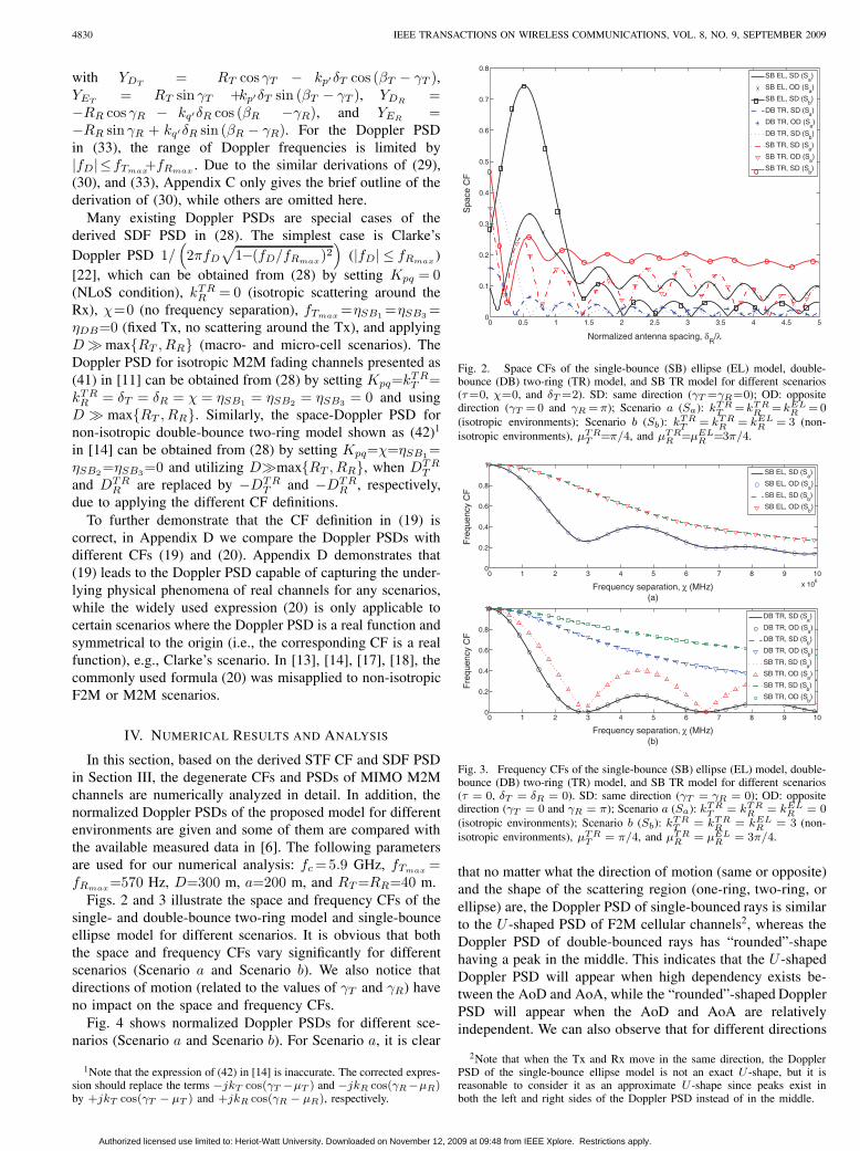
In this section, based on the derived STF CF and SDF PSDin Section III, the degenerate CFs and PSDs of MIMO M2Mchannels are numerically analyzed in detail. In addition, thenormalized Doppler PSDs of the proposed model for differentenvironments are given and some of them are compared withthe available measured data in [6]. The following parametersare used for our numerical analysis: 𝑓𝑐=5.9 GHz, 𝑓𝑇𝑚𝑎𝑥 =𝑓𝑅𝑚𝑎𝑥=570 Hz, 𝐷=300 m, 𝑎=200 m, and 𝑅𝑇=𝑅𝑅=40 m.

Figs. 2 and 3 illustrate the space and frequency CFs of thesingle- and double-bounce two-ring model and single-bounceellipse model for different scenarios. It is obvious that boththe space and frequency CFs vary significantly for differentscenarios (Scenario 𝑎 and Scenario 𝑏). We also notice thatdirections of motion (related to the values of 𝛾𝑇 and 𝛾𝑅) haveno impact on the space and frequency CFs.

Fig. 4 shows normalized Doppler PSDs for different sce-narios (Scenario 𝑎 and Scenario 𝑏). For Scenario 𝑎, it is clear

1Note that the expression of (42) in [14] is inaccurate. The corrected expres-sion should replace the terms −𝑗𝑘𝑇 cos(𝛾𝑇 −𝜇𝑇 ) and −𝑗𝑘𝑅 cos(𝛾𝑅−𝜇𝑅)by +𝑗𝑘𝑇 cos(𝛾𝑇 − 𝜇𝑇 ) and +𝑗𝑘𝑅 cos(𝛾𝑅 − 𝜇𝑅), respectively.

0 0.5 1 1.5 2 2.5 3 3.5 4 4.5 50

0.1

0.2

0.3

0.4

0.5

0.6

0.7

0.8

Normalized antenna spacing, δR

/λ

Spa

ce C

F

SB EL, SD (Sa)

SB EL, OD (Sa)

SB EL, SD (Sb)

DB TR, SD (Sa)

DB TR, OD (Sa)

DB TR, SD (Sb)

SB TR, SD (Sa)

SB TR, OD (Sa)

SB TR, SD (Sb)

Fig. 2. Space CFs of the single-bounce (SB) ellipse (EL) model, double-bounce (DB) two-ring (TR) model, and SB TR model for different scenarios(𝜏=0, 𝜒=0, and 𝛿𝑇 =2). SD: same direction (𝛾𝑇 =𝛾𝑅=0); OD: oppositedirection (𝛾𝑇 =0 and 𝛾𝑅 =𝜋); Scenario 𝑎 (𝑆𝑎): 𝑘𝑇𝑅

𝑇 = 𝑘𝑇𝑅𝑅 = 𝑘𝐸𝐿

𝑅 =0(isotropic environments); Scenario 𝑏 (𝑆𝑏): 𝑘𝑇𝑅


𝑅 = 3 (non-isotropic environments), 𝜇𝑇𝑅

𝑇 =𝜋/4, and 𝜇𝑇𝑅𝑅 =𝜇𝐸𝐿

𝑅 =3𝜋/4.

0 1 2 3 4 5 6 7 8 9 10

x 106

0

0.2

0.4

0.6

0.8

1

Frequency separation, χ (MHz)(a)

Fre

quen

cy C

F

0 1 2 3 4 5 6 7 8 9 100

0.2

0.4

0.6

0.8

1

Frequency separation, χ (MHz)(b)

Fre

quen

cy C

F

DB TR, SD (Sa)

DB TR, OD (Sa)

DB TR, SD (Sb)

DB TR, OD (Sb)

SB TR, SD (Sa)

SB TR, OD (Sa)

SB TR, SD (Sb)

SB TR, OD (Sb)

SB EL, SD (Sa)

SB EL, OD (Sa)

SB EL, SD (Sb)

SB EL, OD (Sb)

Fig. 3. Frequency CFs of the single-bounce (SB) ellipse (EL) model, double-bounce (DB) two-ring (TR) model, and SB TR model for different scenarios(𝜏 = 0, 𝛿𝑇 = 𝛿𝑅 = 0). SD: same direction (𝛾𝑇 = 𝛾𝑅 = 0); OD: oppositedirection (𝛾𝑇 = 0 and 𝛾𝑅 = 𝜋); Scenario 𝑎 (𝑆𝑎): 𝑘𝑇𝑅


𝑅 = 0(isotropic environments); Scenario 𝑏 (𝑆𝑏): 𝑘𝑇𝑅


𝑅 = 3 (non-isotropic environments), 𝜇𝑇𝑅

𝑇 = 𝜋/4, and 𝜇𝑇𝑅𝑅 = 𝜇𝐸𝐿

𝑅 = 3𝜋/4.

that no matter what the direction of motion (same or opposite)and the shape of the scattering region (one-ring, two-ring, orellipse) are, the Doppler PSD of single-bounced rays is similarto the 𝑈 -shaped PSD of F2M cellular channels2, whereas theDoppler PSD of double-bounced rays has “rounded”-shapehaving a peak in the middle. This indicates that the 𝑈 -shapedDoppler PSD will appear when high dependency exists be-tween the AoD and AoA, while the “rounded”-shaped DopplerPSD will appear when the AoD and AoA are relativelyindependent. We can also observe that for different directions

2Note that when the Tx and Rx move in the same direction, the DopplerPSD of the single-bounce ellipse model is not an exact 𝑈 -shape, but it isreasonable to consider it as an approximate 𝑈 -shape since peaks exist inboth the left and right sides of the Doppler PSD instead of in the middle.



−1 −0.8 −0.6 −0.4 −0.2 0 0.2 0.4 0.6 0.8 1−80

−70

−60

−50

−40

−30

−20

−10

0

Normalized Doppler frequency, fD

/(fT

max

+fR

max

)

Nor

mal

ized

Dop

pler

PS

D (

dB)

SB EL, SD (Sa)

SB EL, OD (Sa)

SB EL, SD (Sb)

DB TR, SD (Sa)

DB TR, OD (Sa)

DB TR, SD (Sb)

SB TR, SD (Sa)

SB TR, OD (Sa)

SB TR, SD (Sb)

Fig. 4. Normalized Doppler PSDs of the single-bounce (SB) ellipse (EL)model, double-bounce (DB) two-ring (TR) model, and SB TR model fordifferent scenarios (𝛿𝑇 = 𝛿𝑅 = 0, 𝜒 = 0). SD: same direction (𝛾𝑇 =𝛾𝑅 = 0); OD: opposite direction (𝛾𝑇 = 0 and 𝛾𝑅 = 𝜋); Scenario 𝑎 (𝑆𝑎):𝑘𝑇𝑅𝑇 = 𝑘𝑇𝑅

𝑅 = 𝑘𝐸𝐿𝑅 = 0 (isotropic environments); Scenario 𝑏 (𝑆𝑏): 𝑘𝑇𝑅

𝑇 =𝑘𝑇𝑅𝑅 = 𝑘𝐸𝐿

𝑅 = 3 (non-isotropic environments), 𝜇𝑇𝑅𝑇 = 𝜋/4, and 𝜇𝑇𝑅

𝑅 =𝜇𝐸𝐿𝑅 = 3𝜋/4.

of motion, the Doppler PSDs of double-bounced rays remainunchanged, while the Doppler PSDs of single-bounced rayschange with different ranges of Doppler frequencies. Moreimportantly, we found that the impact of single-bounced raysfrom different rings (ring around the Tx or Rx) on the DopplerPSD are the same for M2M channels when the Tx and Rxmove in opposite directions, leading to the 𝑈 -shaped DopplerPSD for the single-bounce two-ring model. When the Tx andRx move in the same direction, the impact of single-bouncedrays from different rings on the Doppler PSD are different interms of the range of Doppler frequencies, which results inthe double-𝑈 -shaped Doppler PSD for the single-bounce two-ring model. Therefore, we can conclude that a more realisticM2M channel model should take into account the differentcontributions from different rings. However, this has not beenconsidered in all the existing M2M GBSMs, e.g., in [14]. Itis worth mentioning that by setting one terminal fixed (i.e.,𝑓𝑇𝑚𝑎𝑥 = 0), our M2M model can reduce to a F2M model. Inthis case, we studied the Doppler PSD for the correspondingsingle- and double-bounce two-ring F2M models and single-bounce ellipse F2M model, and found that they have thesame 𝑈 -shaped PSD. For brevity, the results regarding F2Mchannels are omitted here. These observations indicates thatthe impact of single- and double-bounced rays on the DopplerPSD are completely different for M2M channels (𝑈 -shapedand “rounded”-shaped, respectively), while they are the samefor F2M channels (𝑈 -shaped). At the end, the comparison ofScenario 𝑎 and Scenario 𝑏 illustrates the significant impact ofangle spreads (related to the values of 𝑘𝑇𝑅𝑇 , 𝑘𝑇𝑅𝑅 , and 𝑘𝐸𝐿𝑅 )and mean angles (related to the values of 𝜇𝑇𝑅𝑇 , 𝜇𝑇𝑅𝑅 , and 𝜇𝐸𝐿𝑅 )on the Doppler PSD.

Figs. 5 and 6 depict the impact of the antenna elementspacing and frequency separation on the Doppler PSD, re-spectively. Fig. 5 shows that the space separation introducesfluctuations in the Doppler PSD no matter what the shape of

−1 −0.8 −0.6 −0.4 −0.2 0 0.2 0.4 0.6 0.8 1−90

−80

−70

−60

−50

−40

−30

−20

−10

0


/(fT

max

+fR

max

)

Nor

mal

ized

spa

ce−

Dop

pler

PS

D (

dB)

SB EL (δT=δ

R=0)

SB EL (δT=δ

R=10λ)

DB TR (δT=δ

R=0)

DB TR (δT=δ

R=10λ)

SB TR (δT=δ

R=0)

SB TR (δT=δ

R=10λ)

Fig. 5. Normalized space-Doppler PSDs of the single-bounce (SB) ellipse(EL) model, double-bounce (DB) two-ring (TR) model, and SB TR modelfor different antenna element spacings in a M2M non-isotropic scatteringenvironment (𝑘𝑇𝑅

𝑇 =𝑘𝑇𝑅𝑅 =𝑘𝐸𝐿

𝑅 =3, 𝜇𝑇𝑅𝑇 =𝜋/4, 𝜇𝑇𝑅

𝑅 =𝜇𝐸𝐿𝑅 =3𝜋/4) with

the Tx and Rx moving in the same direction (𝛾𝑇=𝛾𝑅=0).

−1 −0.8 −0.6 −0.4 −0.2 0 0.2 0.4 0.6 0.8 1−60

−50

−40

−30

−20

−10

0


/(fT

max

+fR

max

)

Nor

mal

ized

freq

uenc

y−D

oppl

er P

SD

(dB

)

SB EL (χ=0)SB EL (χ=10 MHz)DB TR (χ=0)DB TR (χ=10 MHz)SB TR (χ=0)SB TR (χ=10 MHz)

Fig. 6. Normalized frequency-Doppler PSDs of the single-bounce (SB)ellipse (EL) model, double-bounce (DB) two-ring (TR) model, and SB TRmodel for different frequency separations in a M2M non-isotropic scatteringenvironment (𝑘𝑇𝑅

𝑇 =𝑘𝑇𝑅𝑅 =𝑘𝐸𝐿

𝑅 =3, 𝜇𝑇𝑅𝑇 =𝜋/4, 𝜇𝑇𝑅

𝑅 =𝜇𝐸𝐿𝑅 =3𝜋/4) with

the Tx and Rx moving in the opposite direction (𝛾𝑇=0 and 𝛾𝑅=𝜋).

the scattering region is. Fig. 6 illustrates that the frequencyseparation only generates fluctuations in the Doppler PSD forthe double-bounce two-ring model, while for other cases, theimpact of the frequency separation vanishes.

Figs. 7 (a) and (b) show the theoretical Doppler PSDsobtained from the proposed M2M model for different VTDs(low and high) when the Tx and Rx move in opposite direc-tions and same direction, respectively. For further comparison,the measured data taken from Figs. 4 (a) and (c) in [6] arealso plotted in Figs. 7 (a) and (b), respectively. In [6], themeasurement campaigns were performed at a carrier frequencyof 5.9 GHz on an expressway with a low VTD in themetropolitan Atlanta, Georgia area and the maximum Dopplerfrequencies were 𝑓𝑇𝑚𝑎𝑥 = 𝑓𝑅𝑚𝑎𝑥 = 570 Hz. The distancebetween the Tx and Rx was approximately 𝐷 = 300 m and



−1000 −500 0 500 1000−50

−40

−30

−20

−10

0

Doppler frequency, fD

(Hz)

(a)

Nor

mal

ized

Dop

pler

PS

D (

dB)

−1000 −500 0 500 1000−50

−40

−30

−20

−10

0


(Hz)

(b)

Nor

mal

ized

Dop

pler

PS

D (

dB)

Measured, low VTDTheoretical, low VTDTheoretical, high VTD

Measured, low VTDTheoretical, low VTDTheoretical, high VTD

Fig. 7. Normalized Doppler PSDs of the proposed adaptive model fordifferent SISO pico-cell scenarios (𝛿𝑇 = 𝛿𝑅 = 0, 𝜒 = 0): (a) Tx andRx move in opposite directions, (b) Tx and Rx move in the same direction.VTD: vehicular traffic density.

the directions of movement were 𝛾𝑇 = 0, 𝛾𝑅 = 𝜋 (oppositedirection, shown in Fig. 4 (a) in [6]) and 𝛾𝑇 = 𝛾𝑅 = 0(same direction, shown in Fig. 4 (c) in [6]). Both the Txand Rx were equipped with one omnidirectional antenna, i.e.,SISO case. Based on the measured scenarios in [6], we chosethe following environment-related parameters: 𝑘𝑇𝑅𝑇 = 6.6,𝑘𝑇𝑅𝑅 = 8.3, 𝑘𝐸𝐿𝑅 = 5.5, 𝜇𝑇𝑅𝑇 = 12.8∘, 𝜇𝑇𝑅𝑅 = 178.7∘, and𝜇𝐸𝐿𝑅 = 131.6∘ for Fig. 7 (a), and 𝑘𝑇𝑅𝑇 = 9.6, 𝑘𝑇𝑅𝑅 = 3.6,𝑘𝐸𝐿𝑅 =11.5, 𝜇𝑇𝑅𝑇 =21.7∘, 𝜇𝑇𝑅𝑅 =147.8∘, and 𝜇𝐸𝐿𝑅 =171.6∘

for Fig. 7 (b). Considering the constraints of the Riceanfactor and energy-related parameters for different propagationscenarios as mentioned in Section II, we choose the followingparameters in order to fit the measured Doppler PSDs reportedin [6] for the two scenarios with low VTD: 1) 𝐾 = 2.186,𝜂𝐷𝐵=0.005, 𝜂𝑆𝐵1 =0.252, 𝜂𝑆𝐵2 =0.262, and 𝜂𝑆𝐵3 =0.481for Fig. 7 (a); 2) 𝐾 = 3.786, 𝜂𝐷𝐵 = 0.051, 𝜂𝑆𝐵1 = 0.335,𝜂𝑆𝐵2=0.203, and 𝜂𝑆𝐵3=0.411 for Fig. 7 (b). The excellentagreement between the theoretical results and measured dataconfirms the utility of the proposed model. The environment-related parameters for high VTD in Figs. 7 (a) and (b) arethe same as those for low VTD except 𝑘𝑇𝑅𝑇 = 𝑘𝑇𝑅𝑅 = 0.6,which are related to the distribution of moving cars (normally,the smaller values the more distributed moving cars, i.e., thehigher VTD). The Doppler PSDs for high VTD shown inFigs. 7 (a) and (b) were obtained with the parameters 𝐾=0.2,𝜂𝐷𝐵 = 0.715, 𝜂𝑆𝐵1 = 𝜂𝑆𝐵2 = 0.115, and 𝜂𝑆𝐵3 = 0.055.Unfortunately, to the best of the authors’ knowledge, nomeasurement results (e.g., in [4]–[9]) were available regardingthe impact of high VTD (e.g., a traffic jam) on the DopplerPSD.

Comparing the theoretical Doppler PSDs in Figs. 7 (a)and (b), we observe that the VTD significantly affects boththe shape and value of the Doppler PSD for M2M channels.The Doppler PSD tends to be more evenly distributed acrossall Doppler frequencies with a higher VTD. This is becausewith a high VTD, the received power mainly comes from themoving cars around the Tx and Rx from all directions, while

the power of the line-of-sight (LoS) component is not thatsignificant. This means that the received power for differentDoppler frequencies (directions) is more evenly distributed.With a low VTD, the received power from the LoS componentmay be significant, while the power from the moving cars maybe small. Therefore, the power tends to be concentrated onsome Doppler frequencies.

V. CONCLUSION

In this paper, we have proposed a generic and adaptiveGBSM for non-isotropic MIMO M2M Ricean fading channels.By adjusting some model parameters and with the help ofthe newly derived general relationship between the AoA andAoD, the proposed model is adaptable to a wide variety ofM2M propagation environments. In addition, the VTD is forthe first time taken into account in the GBSM for modelingM2M channels. From this model, we have derived the STF CFand the corresponding SDF PSD for non-isotropic scatteringenvironments, where the closed-form expressions are availablein the case of the single-bounce two-ring model for macro-cell and micro-cell scenarios, and the double-bounce two-ringmodel for any scenarios. Based on the derived STF CFs andSDF PSDs, we have further investigated the degenerate CFsand PSDs in detail and found that some parameters (e.g., theangle spread, direction of motion, antenna element spacing,etc.) and the VTD have a great impact on the resulting CFs andPSDs. It has also been demonstrated that for M2M isotropicscenarios, no matter what the direction of motion and shapeof the scattering region are, single-bounced rays will result inthe 𝑈 -shaped Doppler PSD, while double-bounced rays willresult in the “rounded”-shaped Doppler PSD. Finally, it hasbeen shown that theoretical Doppler PSDs match the measureddata in [6], validating the utility of our model.

APPENDIX

A. DERIVATIONS OF (13)–(18)

In this appendix, following the same derivation procedure(i.e., the same newly proposed method), we will derive thesegeneral relationships for the two-ring model in (13)–(16) andthe ellipse model in (17) and (18). In Fig. 1, applying thelaws of cosines and sines to the triangle 𝑂𝑇 𝑠

(𝑛1)𝑂𝑅, weobtain 𝜉2𝑛1

= 𝑅2𝑇 +𝐷2−2𝐷𝑅𝑇 cos𝜙

(𝑛1)𝑇 , 𝑅2

𝑇 = 𝜉2𝑛1+𝐷2+

2𝐷𝜉𝑛1 cos𝜙(𝑛1)𝑅 , and 𝑅𝑇 / sin𝜙

(𝑛1)𝑅 = 𝜉𝑛1/ sin𝜙

(𝑛1)𝑇 . From

the above expressions, we can easily obtain (13) and (14).Similarly, applying the laws of cosines and sines to the triangle𝑂𝑇 𝑠

(𝑛2)𝑂𝑅, we have 𝜉2𝑛2=𝑅2

𝑅+𝐷2+2𝐷𝑅𝑅 cos𝜙

(𝑛2)𝑅 , 𝑅2

𝑅=

𝜉2𝑛2+𝐷2−2𝐷𝜉𝑛2 cos𝜙

(𝑛2)𝑇 , and 𝑅𝑅/ sin𝜙

(𝑛2)𝑇 =𝜉𝑛2/ sin𝜙

(𝑛2)𝑅 .

We can easily obtain (15) and (16) from these expressions.Analogously, applying the laws of cosines and sines to the

triangle 𝑂𝑇 𝑠(𝑛3)𝑂𝑅, we get(𝜉(𝑛3)𝑇

)2=(𝜉(𝑛3)𝑅

)2+𝐷2+2𝐷𝜉

(𝑛3)𝑅

× cos𝜙(𝑛3)𝑅 ,

(𝜉(𝑛3)𝑅

)2=(𝜉(𝑛3)𝑇

)2+𝐷2−2𝐷𝜉

(𝑛3)𝑇 cos𝜙

(𝑛3)𝑇 , and

𝜉(𝑛3)𝑅 / sin𝜙

(𝑛3)𝑇 =𝜉

(𝑛3)𝑇 / sin𝜙

(𝑛3)𝑅 . Based on the above expres-

sions, and the following equalities 𝐷=2𝑓 and 𝜉(𝑛3)𝑇 +𝜉

(𝑛3)𝑅 =2𝑎,

we can get (17) and (18).



B. DERIVATION OF (23)

Considering the von Mises PDF for the two-ring model,applying the following approximate relationships 𝜙(𝑛1)

𝑅 ≈𝜋−Δ𝑇 sin𝜙

(𝑛1)𝑇 and 𝜙

(𝑛2)𝑇 ≈Δ𝑅 sin𝜙

(𝑛2)𝑅 , and substituting (3)

and (6)–(9) into (19), we have


′𝑆𝐵1(2)

𝑝′𝑞′(𝜏, 𝜒)=

[2𝜋𝐼0

(𝑘𝑆𝐵1(2)

𝑇 (𝑅)

)]−1

𝑒𝑗𝐶

𝑆𝐵1(2)

𝑇 (𝑅)√(𝐾𝑝𝑞+1) (𝐾𝑝′𝑞′+1)

×𝜋∫

−𝜋𝑒

(𝐴

𝑆𝐵1(2)

𝑇 (𝑅)cos𝜙

𝑆𝐵1(2)

𝑇 (𝑅)+𝐵

𝑆𝐵1(2)

𝑇(𝑅)sin𝜙

𝑆𝐵1(2)

𝑇 (𝑅)

)𝑑𝜙𝑆𝐵1(2)

𝑇 (𝑅) (35)

where 𝐴𝑆𝐵1(2)

𝑇 (𝑅) , 𝐵𝑆𝐵1(2)

𝑇 (𝑅) , and 𝐶𝑆𝐵1(2)

𝑇 (𝑅) have been given in(24a)–(24f). The definite integrals in the right hand side of

(35) can be solved by using the equality𝜋∫

−𝜋𝑒𝑎 sin 𝑐+𝑏 cos 𝑐𝑑𝑐 =

2𝜋𝐼0(√

𝑎2 + 𝑏2)

[25]. After some manipulation, we can getthe closed-form expression (23).

C. DERIVATION OF (30)

Given 𝑎2+𝑏2=𝑐(𝑑2+𝑒2), after some complex manipulation,

we can rewrite 𝐼0

[√(𝐴𝑆𝐵1(2)

𝑇 (𝑅)

)2+(𝐵𝑆𝐵1(2)

𝑇 (𝑅)

)2]as

𝐼0

⎡⎢⎢⎣𝑗√𝑊𝑆𝐵1(2)

𝑇 (𝑅)

√√√√⎷⎛⎝𝜏 +

𝐷𝑆𝐵1(2)

𝑇 (𝑅)

𝑊𝑆𝐵1(2)

𝑇 (𝑅)

⎞⎠

2

+

⎛⎝ 𝐸

𝑆𝐵1(2)

𝑇 (𝑅)

𝑊𝑆𝐵1(2)

𝑇 (𝑅)

⎞⎠

2⎤⎥⎥⎦ (36)

where 𝑊𝑆𝐵1(2)

𝑇 (𝑅) , 𝐷𝑆𝐵1(2)

𝑇 (𝑅) , and 𝐸𝑆𝐵1(2)

𝑇 (𝑅) have been given in(31b)–(31d). Note that the expression (36) corrects the ex-pressions (38) and (39) in [14]. By applying the Fouriertransform to (23) in terms of the time separation 𝜏 and using

(36) and the equality∞∫0

𝐼0

(𝑗𝛼√𝑥2 + 𝑦2

)cos (𝛽𝑥) 𝑑𝑥 =

cos(𝑦√𝛼2 − 𝛽2

)/√𝛼2 − 𝛽2 [25], we can obtain (30).

D. COMPARISON BETWEEN THE DOPPLER PSDS WITH DIF-FERENT CFS (19) AND (20)

To further clarify which CF definition, (19) or (20), resultsin the correct Doppler PSD to accurately reflect the under-lying physical phenomena of real channels, we first derivethe relationship between the Doppler PSD based on the CF(19), 𝑆ℎ𝑝𝑞ℎ𝑝𝑞 (𝑓𝐷), and the Doppler PSD based on the CF(20), 𝑆ℎ𝑝𝑞ℎ𝑝𝑞 (𝑓𝐷). Considering the equality 𝜌ℎ𝑝𝑞ℎ𝑝𝑞 (𝜏) =𝜌∗ℎ𝑝𝑞ℎ𝑝𝑞

(𝜏) and the Fourier transform relation between the CFand Doppler PSD, we have

𝑆ℎ𝑝𝑞ℎ𝑝𝑞 (𝑓𝐷) = 𝑆∗ℎ𝑝𝑞ℎ𝑝𝑞

(−𝑓𝐷) . (37)

From (37), it is clear that only if 𝑆ℎ𝑝𝑞ℎ𝑝𝑞 (𝑓𝐷) is a real functionand symmetrical to the origin, the equality 𝑆ℎ𝑝𝑞ℎ𝑝𝑞 (𝑓𝐷) =𝑆ℎ𝑝𝑞ℎ𝑝𝑞 (𝑓𝐷) holds. Note that due to the Fourier transform re-lationship, the equality 𝑆ℎ𝑝𝑞ℎ𝑝𝑞 (𝑓𝐷) = 𝑆ℎ𝑝𝑞ℎ𝑝𝑞 (𝑓𝐷) leads tothe equality 𝜌ℎ𝑝𝑞ℎ𝑝𝑞 (𝜏) = 𝜌ℎ𝑝𝑞ℎ𝑝𝑞 (𝜏) and vice versa. We nowproceed the comparison of 𝑆ℎ𝑝𝑞ℎ𝑝𝑞 (𝑓𝐷) and 𝑆ℎ𝑝𝑞ℎ𝑝𝑞 (𝑓𝐷) inthe following two typical scenarios.

Rx (MS) Tx (MS1) Rx (MS2)

Scenario1 Scenario2

3,

TRR

R

k

(a) (b)

Tx (BS)

Fig. 8. Graphical description of (a) Scenario1 and (b) Scenario2.

The first typical scenario, Scenario1, is a non-isotropic F2Mmacro-cell propagation environment (𝑓𝑇𝑚𝑎𝑥=0), as shown inFig. 8(a). We use a one-ring model to represent this scenario,where the ring of scatterers is around the Rx, i.e., mobilestation (MS), and the MS moves toward the direction of theTx, i.e., 𝛾𝑅 = 𝜋. Note that the major amount of scatterersare located in a small part of the ring facing the motion ofthe MS, i.e., 𝜇𝑅=𝜋. The second scenario, Scenario2, is anisotropic M2M propagation environment (𝑘𝑇𝑅𝑇 = 𝑘𝑇𝑅𝑅 = 0),where the Tx and Rx move in opposite directions (𝛾𝑇=0 and𝛾𝑅=𝜋), as shown in Fig. 8(b). Here, a single-bounce two-ring model is used to represent this scenario. For Scenario1,based on (37), the opposite results for the Doppler PSDare expected as shown in Fig. 9, where 𝑘𝑇𝑅𝑅 = 3. Sincethe MS moves toward the majority of received signals, themaximum Doppler PSD should appear at 𝑓𝐷=𝑓𝑅𝑚𝑎𝑥=570 Hz.From Fig. 9, it is clear that the 𝑆ℎ𝑝𝑞ℎ𝑝𝑞 (𝑓𝐷) presents theunderlying physical phenomena for Scenario1. For Scenario2,as expected from (37), the opposite results of the DopplerPSD with respect to the range of Doppler frequencies areillustrated in Fig. 9, where 𝑓𝑇𝑚𝑎𝑥 = 𝑓𝑅𝑚𝑎𝑥 = 570 Hz wereused. Since the Tx and Rx are moving in opposite directions,the Doppler PSD should be limited to the range of Dopplerfrequencies 0≤𝑓𝐷≤1140 Hz, whereas the maximum DopplerPSD exists at 𝑓𝐷 = 0 and 𝑓𝐷 = 𝑓𝑇𝑚𝑎𝑥+𝑓𝑅𝑚𝑎𝑥 = 1140 Hz.Again, from Fig. 9, it is obvious that 𝑆ℎ𝑝𝑞ℎ𝑝𝑞 (𝑓𝐷) reflects theunderlying physical phenomenon for Scenario2. Therefore, wecan conclude that 𝑆ℎ𝑝𝑞ℎ𝑝𝑞 (𝑓𝐷) is able to accurately capturethe underlying physical phenomena of real channels for anyscenarios, while 𝑆ℎ𝑝𝑞ℎ𝑝𝑞 (𝑓𝐷) cannot. It is worth stressing thatfor an isotropic F2M macro-cell scenario (Clarke’s scenario),where no scatterers are around the Tx, we find that thedifference of the Doppler PSD caused by two CF definitionsvanishes, i.e., 𝑆ℎ𝑝𝑞ℎ𝑝𝑞 (𝑓𝐷) = 𝑆ℎ𝑝𝑞ℎ𝑝𝑞 (𝑓𝐷). This is becauseClarke’s scenario has the 𝑈 -shape Doppler PSD, which is areal function and symmetrical to the origin. This seems to bethe reason why the CF (20) was widely misapplied.

REFERENCES

[1] R. Wang and D. Cox, “Channel modeling for ad hoc mobile wirelessnetworks,” in Proc. IEEE VTC’02-Spring, Birmingham, USA, May 2002,pp. 21–25.

[2] F. Kojima, H. Harada, and M. Fujise, “Inter-vehicle communication net-work with an autonomous relay access scheme,” IEICE Trans. Commun.,vol. E83-B, no. 3, pp. 566–575, Mar. 2001.

[3] IEEE P802.11p/D2.01, “Standard for wireless local area networks pro-viding wireless communications while in vehicular environment,” Tech.Rep., Mar. 2007.

[4] J. Maurer, T. Fugen, and W. Wisebeck, “Narrow-band measurement andanalysis of the inter-vehicle transmission channel at 5.2 GHz,” in Proc.IEEE VTC’02-Spring, Birmingham, USA, May 2002, pp. 1274–1278.



−1000 −500 0 500 10000

0.1

0.2

0.3

0.4

0.5

0.6

0.7


(Hz)

Dop

pler

PS

D

Scenario2:

definition in (20)

Scenario2:

definition in (19)

Scenario1:

definition in (20)

Scenario1:

definition in (19)

Fig. 9. Comparison of the Doppler PSDs of Scenario1 and Scenario2 basedon the CF definitions in (19) and (20).

[5] G. Acosta, K. Tokuda, and M. A. Ingram, “Measured joint Doppler-delay power profiles for vehicle-to-vehicle communications at 2.4 GHz,”in Proc. IEEE GLOBECOM’04, Dallas, USA, Nov. 2004, pp. 3813–3817.

[6] G. Acosta and M. A. Ingram, “Six time- and frequency-selective empiricalchannel models for vehicular wireless LANs,” IEEE Veh. Technol. Mag.,vol. 2, no. 4, pp. 4–11, Dec. 2007.

[7] L. Cheng, B. E. Henty, D. D. Stancil, F. Bai, and P. Mudalige, “Mobilevehicle-to-vehicle narrowband channel measurement and characterizationof the 5.9 GHz dedicated short range communication (DSRC) frequencyband,” IEEE J. Select. Areas Commun., vol. 25, no. 8, pp. 1501–1516,Oct. 2007.

[8] I. Sen and D. W. Matolak, “Vehicle-vehicle channel models for the 5-GHz band,” IEEE Trans. Intell. Transp. Syst., vol. 9, no. 2, pp. 235–245,June 2008.

[9] A. Paier, J. Karedal, N. Czink, C. Dumard, T. Zemen, F. Tufvesson,A. F. Molisch, and C. F. Mecklenbrauker, “Characterization of vehicle-to-vehicle radio channels from measurements at 5.2 GHz,” WirelessPers. Commun., June 2008. [Online] http://dx.doi.org/10.1007/s11277-008-9546-6.

[10] J. Maurer, T. Fugen, M. Porebska, T. Zwick, and W. Wisebeck, “Aray-optical channel model for mobile to mobile communications,” COST2100 4th MCM, COST 2100 TD(08) 430, Wroclaw, Poland, Feb. 2008.

[11] A. S. Akki and F. Haber, “A statistical model for mobile-to-mobile landcommunication channel,” IEEE Trans. Veh. Technol., vol. 35, no. 1, pp.2–10, Feb. 1986.

[12] A. S. Akki, “Statistical properties of mobile-to-mobile land communi-cation channels,” IEEE Trans. Veh. Technol., vol. 43, no. 4, pp. 826–831,Nov. 1994.

[13] M. Patzold, B. O. Hogstad, and N. Youssef, “Modeling, analysis, andsimulation of MIMO mobile-to-mobile fading channels,” IEEE Trans.Wireless Commun., vol. 7, no. 2, pp. 510–520, Feb. 2008.

[14] A. G. Zajic and G. L. Stuber, “Space-time correlated mobile-to-mobilechannels: modeling and simulation,” IEEE Trans. Veh. Technol., vol. 57,no. 2, pp. 715–726, Mar. 2008.

[15] A. F. Molisch, “A generic model for MIMO wireless propagationchannels in macro- and microcells,” IEEE Trans. Signal Process., vol. 51,no. 1, pp. 61–71, Jan. 2004.

[16] C.-X. Wang, M. Patzold, and Q. Yao, “Stochastic modeling and simu-lation of frequency correlated wideband fading channels,” IEEE Trans.Veh. Technol., vol. 56, no. 3, pp. 1050–1063, May 2007.

[17] A. Abdi and M. Kaveh, “A space-time correlation model for multiele-ment antenna systems in mobile fading channels,” IEEE J. Select. AreasCommun., vol. 20, no. 3, pp. 550–560, Apr. 2002.

[18] X. Cheng, C.-X. Wang, and D. I. Laurenson, “A generic space-time-frequency correlation model and its corresponding simulation model forMIMO wireless channels,” in Proc. EuCAP’07, Edinburgh, UK, Nov.2007, pp. 1–6.

[19] A. Papoulis and S. U. Pillai, Probability, Random Variables and Stochas-tic Processes, 4th ed. New York: McGraw Hill, 2002.

[20] M. Patzold and N. Youssef, “Modeling and simulation of direction-selective and frequency-selective mobile radio channels,” International J.Electron. and Commun., vol. 55, no. 6, pp. 433–442, Nov. 2001.

[21] P. Y. Chen and H. J. Li, “Modeling and applications of space-timecorrelation for MIMO fading signals,” IEEE Trans. Veh. Technol., vol.56, no. 4, pp. 1580–1590, July 2007.

[22] G. L. Stuber, Principles of Mobile Communication, 2nd ed. Boston:Kluwer Academic Publishers, 2001.

[23] A. Abdi, J. A. Barger, and M. Kaveh, “A parametric model for thedistribution of the angle of arrival and the associated correlation functionand power spectrum at the mobile station,” IEEE Trans. Veh. Technol.,vol. 51, no. 3, pp. 425–434, May 2002.

[24] S. Wang, A. Abdi, J. Salo, H. M. EL-Sallabi, J. W. Wallace, P.Vainikainen, and M. A. Jensen, “Time-varying MIMO channels: para-metric statistical modeling and experimental results,” IEEE Trans. Veh.Technol., vol. 56, no. 4, pp. 1949–1963, July 2007.

[25] I. S. Gradshteyn and I. M. Ryzhik, Table of Integrals, Series, andProducts, 6th ed. Boston: Academic, 2000.

Xiang Cheng (S’05) received the BSc and MEngdegrees in communication and information systemsfrom Shandong University, China, in 2003 and 2006,respectively. Since October 2006, he has been aPhD student at Heriot-Watt University, Edinburgh,UK. His current research interests include mobilepropagation channel modeling and simulation, mul-tiple antenna technologies, mobile-to-mobile com-munications, and cooperative communications. Hehas published more than 20 research papers injournals and conference proceedings. Mr. Cheng was

awarded the Postgraduate Research Prize from Heriot-Watt University in 2007and 2008, respectively, for academic excellence and outstanding performance.He served as a TPC member for IEEE HPCC2008 and IEEE CMC2009.

Cheng-Xiang Wang (S’01-M’05-SM’08) receivedthe BSc and MEng degrees in communicationand information systems from Shandong University,China, in 1997 and 2000, respectively, and the PhDdegree in wireless communications from AalborgUniversity, Denmark, in 2004.

Dr Wang has been a lecturer at Heriot-Watt Uni-versity, Edinburgh, UK since 2005. He is also anhonorary fellow of the University of Edinburgh, UK,a guest researcher of Xidian University, China, andan adjunct professor of Guilin University of Elec-

tronic Technology, China. He was a research fellow at the University of Agder,Norway, from 2001-2005, a visiting researcher at Siemens AG-Mobile Phones,Munich, Germany, in 2004, and a research assistant at Technical University ofHamburg-Harburg, Germany, from 2000-2001. His current research interestsinclude wireless channel modelling and simulation, cognitive radio networks,mobile-to-mobile communications, cooperative communications, cross-layerdesign, MIMO, OFDM, UWB, wireless sensor networks, and (beyond) 4G. Hehas published 1 book chapter and over 110 papers in journals and conferences.

Dr Wang serves as an editor for IEEE TRANSACTIONS ON WIRELESS

COMMUNICATIONS, WILEY WIRELESS COMMUNICATIONS AND MOBILECOMPUTING JOURNAL, WILEY SECURITY AND COMMUNICATION NET-WORKS JOURNAL, and JOURNAL OF COMPUTER SYSTEMS, NETWORKS,AND COMMUNICATIONS. He served or is servings as a TPC chair for CMC2009, publicity chair for CrownCom 2009, TPC symposium co-chair forIWCMC 2009, General Chair for VehiCom 2009, and TPC vice-chair ormember for more than 35 international conferences. Dr Wang is listed inDictionary of International Biography 2008 and 2009, Who’s Who in theWorld 2008 and 2009, Great Minds of the 21st Century 2009, and 2009 Manof the Year.

David I. Laurenson (M’90) is currently a SeniorLecturer at The University of Edinburgh, Scotland.His interests lie in mobile communications: at thelink layer this includes measurements, analysis andmodelling of channels, whilst at the network layerthis includes provision of mobility managementand Quality of Service support. His research ex-tends to practical implementation of wireless net-works to other research fields, such as predic-tion of fire spread using wireless sensor networks(http://www.firegrid.org), to deployment of commu-

nication networks for distributed control of power distribution networks. Heis an associate editor for Hindawi journals, and acts as a TPC member forinternational communications conferences. He is a member of the IEEE andthe IET.



Sana Salous (M’95) received the B.E.E. degreefrom the American University of Beirut, Beirut,Lebanon, in 1978 and the M.Sc. and Ph.D. degreesfrom the University of Birmingham, Birmingham,U.K., in 1979 and 1984, respectively. She was anAssistant Professor with Yarmouk University, Irbid,Jordan, until 1988 and a Research Associate withthe University of Liverpool, Liverpool, U.K., until1989, at which point, she took up a lecturer postwith the Department of Electronic and ElectricalEngineering, University of Manchester Institute of

Science and Technology (UMIST), Manchester, U.K. In 2003 she took upthe Chair in Communications Engineering with the School of Engineering,Durham University, Durham, U.K, where she is currently the Director of theCentre for Communications Systems.

Athanasios V. Vasilakos (M’89) is currently Pro-fessor at the Dept. of Computer and Telecommuni-cations Engineering, University of Western Mace-donia, Greece, and Visiting Professor at the Grad-uate Programme of the Dept. of Electrical andComputer Engineering, National Technical Univer-sity of Athens (NTUA). He is coauthor (with W.Pedrycz) of the books Computational Intelligencein Telecommunications Networks (CRC press, USA,2001), Ambient Intelligence, Wireless Networking,Ubiquitous Computing (Artech House, USA, 2006),

coauthor (with M. Parashar, S. Karnouskos, W. Pedrycz) Autonomic Com-munications (Springer, to appear ), Arts and Technologies (MIT Press,to appear), coauthor (with Yan Zhang, Thrasyvoulos Spyropoulos) DelayTolerant Networking (CRC press, to appear), coauthor (with M. Anastasopou-los) Game Theory in Communication Systems (IGI Inc, USA, to appear).He has published more than 200 articles in top international journals (i.eIEEE/ACM TRANSACTIONS ON NETWORKING, IEEE TRANSACTIONS ON

INFORMATION THEORY, IEEE JOURNAL ON SELECTED AREAS IN COM-MUNICATIONS, IEEE TRANSACTIONS ON WIRELESS COMMUNICATIONS,IEEE TRANSACTIONS ON NEURAL NETWORKS, IEEE TRANSACTIONS ON

SYSTEMS, MAN, AND CYBERNETICS, IEEE T-ITB, IEEE T-CIAIG, etc)and conferences. He is the Editor-in-chief of the Inderscience Publishersjournals: INTERNATIONAL JOURNAL OF ADAPTIVE AND AUTONOMOUS

COMMUNICATIONS SYSTEMS (IJAACS), INTERNATIONAL JOURNAL OFARTS AND TECHNOLOGY. He was or is at the editorial board of morethan 20 international journals including: IEEE COMMUNICATIONS MAGA-ZINE (1999-2002 and 2008-), IEEE TRANSACTIONS ON SYSTEMS, MANAND CYBERNETICS (TSMC, Part B, 2007-), IEEE TRANSACTIONS ONWIRELESS COMMUNICATIONS (invited), IEEE TRANSACTIONS ON INFOR-MATION THEORY IN BIOMEDICINE (TITB,2009-), etc. He chairs severalconferences, e.g., ACM IWCMC’09, ICST/ACM Autonomics 2009. He isa chairman of the Telecommunications Task Force of the Intelligent SystemsApplications Technical Committee (ISATC) of the IEEE Computational Intel-ligence Society (CIS). Senior Deputy Secretary-General and fellow memberof ISIBM www.isibm.org (International Society of Intelligent BiologicalMedicine (ISIBM)). He is member of the IEEE and ACM.


4824 ieee transactions on wireless communications,...

Documents