a a ay a - bpa.gov

POTENTIAL ANALYTICS FOR NON-ROUTINE

ADJUSTMENTS

Prepared for BONNEVILLE POWER ADMINISTRATION

Keshmira McVey

Prepared by SBW CONSULTING, INC. 2820 Northup Way, Suite 230 Bellevue, WA 98004

April 30, 2018

Potential Analytics for Non-Routine Adjustments

SBW Consulting, Inc. 1

1. INTRODUCTION

Non-routine changes in building energy use are those that are not attributable to changes in the independent variables used in the baseline model, or to the efficiency measures that were installed. In the case of a non-routine event, the savings determined by subtracting the metered use in in the performance period from the baseline-predicted load may have to be adjusted to accurately determine the savings due to the installed measures.1 Figure 1 illustrates the presence of a potential non-routine event, as indicated by a history of the building’s metered demand.

Figure 1. Six Months of Electrical Meter Data

Toward the end of the data, there is a dip indicating a reduction of demand during some hours of the day. Figure 2 is a heat map chart that shows it more clearly. Figure 2 shows the model standardized residuals—the difference between the modeled (expected) and actual kW, in number of standard deviations. The darker the color, the greater the difference between the model and metered values, with relatively low metered energy use shown in green and relatively high metered energy use shown in yellow-to-red.

From 6 am to 10 PM for the days of Monday May 12 through Friday, May 23, the energy use is 17% lower than expected.

If this change in energy use is not part of normal operations, it is a “Non-routine event,” and then it should be accounted for in estimating energy savings.

Some of the more frequently encountered types of non-routine events in commercial buildings include, but are not limited to:

1 The preceding text, and other portions of the first two sections in this document are taken from draft, unpublished guidance

for program level M&V plans using “normalized meter-based savings estimation” in California.

12/1

/201

3

12/3

1/2

01

3

1/3

0/2

01

4

3/2

/20

14

4/1

/20

14

5/2

/20

14

Mete

red

kW


2 SBW Consulting, Inc.

Services # of rooms/beds

food cooking/preparation

# of registers

#of workers

Equipment loads # of computers

# of walk-in or standard refrigeration units or open and closed cases

# of MRIs

# or capacity of HVAC units

Operations hours of operation

weekend operations

heating and cooling setpoints

system control strategies

Site characteristics size

% of building heated and cooled

envelope changes



Figure 2. Heat Map of Model Residuals

Hour of DayHour

Date 0 1 2 3 4 5 6 7 8 9 10 11 12 13 14 15 16 17 18 19 20 21 22 23

Tue, 4/1/2014

Wed, 4/2/2014

Thu, 4/3/2014

Fri, 4/4/2014

Sat, 4/5/2014

Sun, 4/6/2014

Mon, 4/7/2014

Tue, 4/8/2014

Wed, 4/9/2014

Thu, 4/10/2014

Fri, 4/11/2014

Sat, 4/12/2014

Sun, 4/13/2014

Mon, 4/14/2014

Tue, 4/15/2014

Wed, 4/16/2014

Thu, 4/17/2014

Fri, 4/18/2014

Sat, 4/19/2014

Sun, 4/20/2014

Mon, 4/21/2014

Tue, 4/22/2014

Wed, 4/23/2014

Thu, 4/24/2014

Fri, 4/25/2014

Sat, 4/26/2014

Sun, 4/27/2014

Mon, 4/28/2014

Tue, 4/29/2014

Wed, 4/30/2014

Thu, 5/1/2014

Fri, 5/2/2014

Sat, 5/3/2014

Sun, 5/4/2014

Mon, 5/5/2014

Tue, 5/6/2014

Wed, 5/7/2014

Thu, 5/8/2014

Fri, 5/9/2014

Sat, 5/10/2014

Sun, 5/11/2014

Mon, 5/12/2014

Tue, 5/13/2014

Wed, 5/14/2014

Thu, 5/15/2014

Fri, 5/16/2014

Sat, 5/17/2014

Sun, 5/18/2014

Mon, 5/19/2014

Tue, 5/20/2014

Wed, 5/21/2014

Thu, 5/22/2014

Fri, 5/23/2014

Sat, 5/24/2014

Sun, 5/25/2014

Mon, 5/26/2014

Tue, 5/27/2014

Wed, 5/28/2014

Thu, 5/29/2014

Fri, 5/30/2014

Sat, 5/31/2014



2. A FRAMEWORK FOR ASSESSING NON-ROUTINE EVENTS

Non-routine events may be characterized as temporary or permanent, as load added or removed, and as constant or variable. A framework of assessing non-routine events may include

1. Determine whether an event is present

2. Determine whether the impact of the event is material, meriting quantification and adjustment (the threshold for what is considered ‘material’ should be specified in the M&V Program Plan)

3. Determine whether the event is temporary or permanent. Temporary events may be removed from the data set, however no more than 25% of the measured data should be removed, per ASHRAE Guideline 14, provided that a justifiable reason is provided.

4. Determine whether the event represents a constant or variable load

5. Determine whether the event represents added or removed load

6. Based on #3-5, the approach to measuring and quantifying the impact of the event may be determined.

Several methods may be used to determine whether an event is present. These include but are not limited to inspection of meter data, time series change detection or breakout analysis, periodic site visits and short term measurements, and site surveys.

Determination of whether the impact of the event is material depends on engineering expertise, and the magnitude of the thresholds that are defined in the M&V Program plan.

Permanent events are those that are expected to last through the duration of the M&V analysis period.

Constant loads are understood to be those that do not fluctuate or change during a period of interest, such as when in the ‘on’ state.

Added loads are those that increase site energy consumption, while removed loads decrease site energy consumption.

Analogous to detecting the presence of an event, several methods may be used to quantify the impact or magnitude of the event. These include but are not limited to, engineering calculations, IPVMP Options A and B, simulation models, time series analysis of residuals, and the use of indicator variables in models fit to data before and after the event.

David Jump has characterized some of the various methods for quality and cost as follows:

Engineering calcs+ assumptions (low quality/cost)

Engineering calcs+ logged data (med-high quality/cost)

Analysis of before/after NRE using metered data (high quality/low cost)



3. TREATMENT OF NON-ROUTINE EVENTS: ANALYTICS

FOR ASSOCIATED NON-ROUTINE ADJUSTMENTS

3.1. General Approaches

It is usually worthwhile to review the model residuals. Analysis of the residuals may help support identification of non-routine events, and often quantification of their impacts. Figures 1 and 2 show an example of identification of a NR event.

If the timing of the non-routine change is not concurrent with other changes, and the signal-to-noise ratio in the data is sufficient for the quantification, there are multiple possible ways these changes can be quantified from the data, and they can include analysis of uncertainty. Here are some possibilities.

Look at the time series of residuals for a model that includes the time period of change, and estimate the magnitude of the change from the change in the residuals.

Use a pre-post model with a ‘mini baseline’ and ‘mini post’ period. The mini baseline is the shorter time period that exists within a baseline or reporting period, and is prior to the NR change. The mini post is similar—for a NR change that is ongoing, it is the shorter time period within a baseline or post period that includes the NR change. The pre-post model uses an indicator variable for the mini post period, and the coefficient on the indicator variable is the NR event impact. This is simply a more robust method of looking at the time series of residuals.

For a change of long duration, especially one that is ongoing through the time period, e.g. baseline period: Treat the time periods around the non-routine change as a mini baseline and a mini post period, and model the change using by subtracting the mini post period energy use from an adjusted baseline developed from the mini baseline period. This can be done using either a forecast or backcast approach, depending upon which mini period has better coverage for the independent variables.

For a temporary NR change of relatively short duration: Model the entire period (e.g. baseline period) excluding the portion of the period that includes the non-routine change. Use this model conjunction with the independent variable(s) for the times that include the non-routine change to estimate energy use for the entire period as if the non-routine change had not occurred. Subtract this estimate from the actual energy use for the period to estimate the impact of the change.

The first two approaches are likely best if the non-routine adjustment is not expected to have a relationship to weather. The third approach may be better if the non-routine adjustment is expected to be related to weather, but it may suffer from inadequate data in both the mini-baseline and mini-post periods. In all cases, the analysis will usually need to be appropriately extrapolated to get the effect over a full year.



Combinations of these approaches are also possible, and perhaps better. For example, a “fully qualified” pre-post model could include coefficients for additional weather and time relationships, as well as a coefficient on the indicator variable for the NR event impact.

LBNL is researching identification and quantification of NR events and impacts. BPA Technical Innovation Project 389, Realizing High-accuracy Low-cost Measurement and Verification for Deep Cost Savings, includes two relevant tasks:

Task 2. Automated identification of non-routine adjustments: Develop open-source, automated methods to identify the potential need for non-routine adjustments based on interval electric data and weather.

Task 3. Standardized quantification of non-routine adjustments: Develop standard methods to quantify commonly encountered non-routine adjustments, e.g. changes in occupancy, changes in operating hours, changes in computer loads, changes to building area based on the building type.

At this time, the results have been discussed in presentations, but no formal documents have been made public.

3.2. Data Analysis Suggestions

How a non-routine event should be handled depends upon when it occurs and what affects its impact.

Timing During Baseline Period

Interim Period (Between Baseline and Reporting Period)

During Reporting Period

Duration Temporary

Permanent

Impact Correlations Constant

Varies with Time (e.g. with Time of Day or Day of Week)

Varies with Weather

Varies with Time and Weather

Varies with Other Variables (not covered herein)

A constant impact should be clear: there is a load of constant kW (or other utility), all hours, that has been added or removed from the meter.

An impact that varies with time is one for which the kW varies by time of day or time of week. For example, in an office building, there is a tenant change and the new tenant’s office hours differ from the prior tenant’s hours. Since tenant kW varies over time anyway, as people arrive,



leave for lunch, and leave at the end of the day, the new tenant’s kW will vary over time as well, but at a different magnitude and time than the prior tenant. (There could be weather-related impacts on this example as well.)

An example where the impact varies only with weather might be the addition of a computer server room with a constant cooling load. Although the load is constant, the heat rejection will vary with the outside temperature (and humidity if evaporatively cooled), and so is varying with weather.

A load that varies with both time and weather could be the tenant change mentioned above, perhaps also in conjunction with a revised HVAC system to serve the new tenant.

3.2.1. Baseline, temporary

Eliminate NR event from baseline data if coverage factor requirements2 for baseline can still be met. Calculate avoided energy use and normalized savings normally.

If coverage factor cannot be met eliminating NR event from data, then follow the suggestions below for a temporary NR event in the baseline period.

3.2.1.1. Baseline, temporary, constant NR event load

The following approach, and similar approaches to follow, are the same as using a pre-post model. In this approach, indicator variables are used for the NR event load, the same as would be done with a pre-post model. However, this approach uses a traditional forecast model, iterating to get the same effect as using a pre-post model, while still using tools designed for forecast models. Example 2 in Section 4.2 will demonstrate this.

Make initial estimate of NR event load.

Subtract NR event load from measured kW.

Re-estimate model.

For NR event period, add NR event load to model predictions.

Check total modeled NR event period energy vs. measured kWh for NR event period energy.

Adjust NR event load to make total modeled NR event period energy = measured NR event period energy.

Iterate as necessary.

2Coverage factor pertains to program-required percentage of typical annual range of an independent variable used in the

model. E.g., for outside air temperature, if the climate has a typical range of temperatures from 22 to 103 ºF, then if the minimum temperature in the baseline period is 22 ºF or lower, and the maximum is 103 ºF or higher, by a simple definition the coverage factor would be 100%. More detailed, or different, definitions of coverage factor are possible.



Verify that NR event period residuals indicate no significant relationship to time or weather.

Add 2 to the number of parameters in the model (one for the indicator variable for NR event period, and one for the NR event load) and re-estimate model statistics.

3.2.1.2. Baseline, temporary, NR event load varying with time

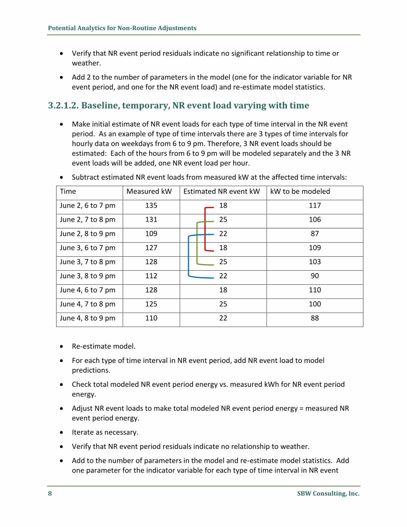
Make initial estimate of NR event loads for each type of time interval in the NR event period. As an example of type of time intervals there are 3 types of time intervals for hourly data on weekdays from 6 to 9 pm. Therefore, 3 NR event loads should be estimated: Each of the hours from 6 to 9 pm will be modeled separately and the 3 NR event loads will be added, one NR event load per hour.

Subtract estimated NR event loads from measured kW at the affected time intervals:

Time Measured kW Estimated NR event kW kW to be modeled

June 2, 6 to 7 pm 135 18 117

June 2, 7 to 8 pm 131 25 106

June 2, 8 to 9 pm 109 22 87

June 3, 6 to 7 pm 127 18 109

June 3, 7 to 8 pm 128 25 103

June 3, 8 to 9 pm 112 22 90

June 4, 6 to 7 pm 128 18 110

June 4, 7 to 8 pm 125 25 100

June 4, 8 to 9 pm 110 22 88

Re-estimate model.

For each type of time interval in NR event period, add NR event load to model predictions.

Check total modeled NR event period energy vs. measured kWh for NR event period energy.

Adjust NR event loads to make total modeled NR event period energy = measured NR event period energy.

Iterate as necessary.

Verify that NR event period residuals indicate no relationship to weather.

Add to the number of parameters in the model and re-estimate model statistics. Add one parameter for the indicator variable for each type of time interval in NR event



period, e.g. 3 for hourly data on weekdays from 6 to 9 pm. Add one for the NR event load for each type of time interval.

3.2.1.3. Baseline, temporary, NR event load varying with weather

If the NR event is of sufficiently short duration, the rest of the data may be sufficient to meet data coverage requirements for a quality model. In this case, just remove the NR event from the data, and model using

Depending on the duration of the NR event, this type of NR event load may mean that a data coverage requirement for weather cannot be met: Specifying a different weather relationship for the NR event period effectively means that the NR event period is excluded from the model.

The analyst could choose to accept the failure to meet the coverage factor, with justification. Alternatively, the weather coefficients for the NR event period could be constrained by (1) engineering knowledge of the changes during the NR event period and (2) by the weather coefficients for other parts of the model.

In many cases, the approach described in Section 3.2.1.2 may be sufficiently close, with a check showing that the relationship to weather is minimal after adjusting the time-related loads to match the data.

3.2.1.4. Baseline, temporary, NR event load varying with both time and weather

The handling of this is similar as for a NR event load varying with just weather, but additional parameters are needed to handle the time-related changes.

3.2.2. Baseline, permanent

Since the change is permanent, the NR event is really the part of the baseline before the change, and the calculations for NR behavior should apply to the part of the baseline period that is before the change. Therefore, the calculations can follow the same approach as for temporary NR events occurring during the baseline.

3.2.3. Interim, temporary

All temporary NR events in the interim period can be ignored.

3.2.4. Interim, permanent

Permanent changes that start in the interim period affect the difference between baseline and reporting period consumption, and hence must be analyzed. In many cases, a change that occurs that is not part of the efficiency improvements will not be able to be distinguished in time from the efficiency improvements. Therefore, the impact of changes that occur in the



interim period will often need to be estimated using engineering calculations rather than data analysis.

Further research is needed for those cases where the NR changes can be separated from the efficiency improvements. To use analytics to estimate the impact of permanent NR changes during the interim period, custom models are likely needed.

3.2.5. NR Events in the Reporting Period

Whether or not to account for a NR event in the reporting (post) period depends upon whether the M&V savings to be estimated are Avoided Energy Use or Normalized Savings. For Normalized Savings, the NR event must always be taken into consideration. For Avoided Energy Use, it depends upon the program definition of savings: If savings are defined as based solely on the actual energy use in the reporting period, then the NR event does not matter. If savings are defined based on normal/typical operation in the reporting period, the temporary NR event must be taken into consideration.

For the situations where the NR event must be taken into consideration, a post period model should be created, and the same suggestions as for a baseline event should be applied to estimate the impact of the NR event.

3.2.5.1. Post, temporary

Follow the suggestions for Baseline, temporary.

3.2.5.2. Post, permanent

Follow the suggestions for Baseline, permanent.



4. EXAMPLES USING A FEW DIFFERENT APPROACHES

The following two examples show how different approaches can be used to estimate the impact of a schedule change. The examples were chosen as an edge case—a case where the NR change was small, but statistically significant.

The example uses a synthetic data set with the following characteristics:

1. All days of the week have the same schedule.

2. Occupancy is from 7 AM to 4 PM. This occupancy period was defined for the model.

3. Occupied period demand is 100 kW + 1 kW per ºF over 60 ºF, and 100 kW for colder temperatures.

4. Unoccupied period demand is 80 kW with no weather dependency.

5. Randomness is included using a normal distribution with a standard deviation of 15 kW about the demand calculated per 3, 4, and 5.

For the first example, Occupancy was extended from 7 AM until 6 PM, instead of 7 AM to 4 PM, in May only. This was a NR schedule change that is not expected to recur. This example is of the type described in Section 3.2.1.3. Baseline, temporary, NR event load varying with weather. The extra hours fall in the Unoccupied period as defined for the model in item 2. Hence, they should not fit the data as well as the other points that actually represent operation during unoccupied times.

For the second example, Occupancy was extended from 7 AM until 6 PM, instead of 7 AM to 4 PM, starting in May and continuing through the rest of the (baseline) period. This was a permanent NR schedule change.



4.1. Example 1—Temporary Schedule Change

The data for the occupied and unoccupied periods for Example 1 are shown in Figures 4 and 5.

Figure 3. Data for Occupied Period With Temporary Schedule Change

Figure 4. Data for Previously Unoccupied Period With Temporary Schedule Change

0

20

40

60

80

100

120

140

160

180

20 30 40 50 60 70 80 90 100 110

Ele

ctr

ical

De

ma

nd

, k

W

Outside Air Temperature, ºF

Occ

0

20

40

60

80

100

120

140

160

180

20 30 40 50 60 70 80 90 100 110

Ele

ctr

ical

De

ma

nd

, k

W


Unocc



4.1.1. Visual Detection of the Change

Since, in May, the occupied period extends 2 hours later, it extends into what was defined for the model as the unoccupied period. Therefore, the points associated with the non-routine change are within Figure 4. Since there were 31 days in May, and occupancy was extended 2 hours, there are 62 hours of higher use. Looking at Figure 4, some hours that seem high are apparent, but it is not at all obvious solely from Figure 4 that there are 62 high-use hours.

4.1.1.1. Hourly Model

Because of the greater information, these types of non-routine changes are best detected with an hourly model. Changes that affect all hours of the day may be as easily detected with a daily model.

Heat Map of Standardized Residuals

This may usually be the best way to visually detect the change. Figure 5 shows a heat map covering 51 days around and including the change, with the latest dates at the top. The values in the cells is the number of standardized residuals (standard deviations) the actual kW was above the kW predicted from the model.



Figure 5. Heat Map of Standardized Residuals

Hour of Day

Avg kW May add 2hours Std ResidHour

Date 0 1 2 3 4 5 6 7 8 9 10 11 12 13 14 15 16 17 18 19 20 21 22 23

Thu, 6/5/2014 1.4 -0 2.2 0.2 -2 0 -1 2.6 1.9 -1 -0 -1 -0 -1 -0 -1 -1 0.5 0.1 0.8 -1 -0 -0 -0

Wed, 6/4/2014 0.4 1.4 0.3 0.2 0.8 1.2 0.2 0.4 0.2 0.4 -0 -0 0.8 -1 -0 -0 -1 -1 -2 -0 -0 -1 -1 0.2

Tue, 6/3/2014 0.3 0.3 0.4 -1 0.9 0.5 -1 0.1 -0 -0 -1 -1 -1 -1 0.1 1.7 0.4 -1 1.1 -0 0.3 -1 0 -1

Mon, 6/2/2014 0.7 -1 -1 -1 -1 -0 -0 1 -0 0.1 0.1 1.3 -0 -1 -0 -1 0.7 -1 0.8 -0 1 -2 1 -1

Sun, 6/1/2014 1.2 2.3 1.8 0.5 -1 -1 0.9 -2 0 -1 1 0.7 -1 -1 -1 0.7 -0 -0 0.9 1.4 0 -0 -1 -0

Sat, 5/31/2014 0.5 -0 -0 0.9 -1 -1 1.5 1.7 -1 -1 0.7 -1 -1 0.3 1.5 2 1.7 0.4 4.1 1.8 0.4 0.6 -2 0.6

Fri, 5/30/2014 0.5 0.1 0.5 -1 -1 -0 0.3 0.5 1.4 0.6 -1 -1 -2 1.3 -0 -0 0.6 0.5 2.1 1.9 1.5 -0 1 -1

Thu, 5/29/2014 -1 0.3 -0 0.9 -1 -1 -0 -0 -0 2.2 -2 -0 0.4 1 -2 0.9 1.2 0.2 3.7 0.1 -0 1.5 -0 0.3

Wed, 5/28/2014 -0 -1 -2 -1 -0 2.7 0.4 0.7 1.2 -0 -0 0.9 1.4 -0 -1 0.4 0.2 -1 3 3.7 -0 -0 1 0.2

Tue, 5/27/2014 -0 -0 0.3 -2 1 -1 0.5 1.3 -1 -1 0.7 -0 0.9 0.4 -1 0.8 1.1 0.5 4 2 -1 -1 -0 0.8

Mon, 5/26/2014 -2 1.2 1.6 1.4 -2 0 2.4 -0 -0 0.8 -0 0.1 0.8 1.4 -0 0.3 0.7 0.3 5.2 3.4 0.1 -1 0.5 1

Sun, 5/25/2014 -2 -1 -1 0.8 -0 -1 0.9 0.6 1.9 -1 -1 -0 -1 -0 -0 -0 -0 0.1 3.2 1.9 0.4 -1 1.3 1

Sat, 5/24/2014 0.4 -0 -1 1.3 -0 -0 0.6 1.7 0.2 0 -1 -0 1.4 0.1 1 -1 0.3 -0 5 1.1 0.9 -0 -0 0.1

Fri, 5/23/2014 -0 -0 -1 1.4 2 -2 -0 0.3 -1 0 -1 -0 1.6 1.4 -1 -0 -0 1.1 3.9 1.4 0.5 -1 0.3 0.8

Thu, 5/22/2014 -0 -0 -0 -0 0.1 0.2 -0 -1 -0 0.8 -1 0.5 0.2 0.7 -0 2 0.1 0.2 1.8 1.5 -1 -0 0.8 0.1

Wed, 5/21/2014 -0 -0 1.1 -0 0.4 -1 2.4 1.2 -0 0.8 0.9 0.6 0.2 1 -0 0.6 1.4 -0 2.6 2.4 -1 -1 -1 0.3

Tue, 5/20/2014 -0 -1 0.4 -1 -1 0.2 -1 -1 0.6 -1 -3 -0 -1 -0 -1 -0 -0 -0 2.4 -1 -0 -1 -1 0.1

Mon, 5/19/2014 0.9 -1 -0 -1 2.6 -0 0.3 0.2 0.5 1.1 -0 -1 -1 -0 2.2 -2 1 0.9 1.8 1 -1 0.5 -1 0.8

Sun, 5/18/2014 -0 -1 -1 -1 -1 -1 0.6 -1 0.4 -1 -2 0.2 1.3 -0 0.2 1.1 -0 -1 4.9 1.4 -1 0 -0 -0

Sat, 5/17/2014 -1 1 -0 -0 0.1 -0 0.3 -0 -1 -0 0.3 1 -1 2.2 -1 1.5 1 1.9 4.2 3.6 -0 1 -1 0.7

Fri, 5/16/2014 1.9 -1 -1 -0 0.5 0.6 -1 -1 0.7 0.6 -0 -0 -1 -1 -0 0.1 -1 0.7 3.7 2.7 0.2 -0 -1 -1

Thu, 5/15/2014 0.2 0.6 0.7 -0 -1 0.4 -1 2.3 -2 -0 -0 -1 -0 -1 -1 0.4 -1 0.3 5.8 5.5 1 0.2 -2 0.1

Wed, 5/14/2014 2 -2 0.9 -2 0.4 -0 0 -3 -1 0.2 -0 2.3 0.4 -2 0.1 -1 0.8 2.2 5.7 4 -0 -0 1.6 -0

Tue, 5/13/2014 0.8 -1 -1 -1 0.9 -0 -1 0.2 -2 0.8 2 -1 -0 -1 -0 -0 0.8 0.3 5.5 1.9 0.4 -2 -1 -1

Mon, 5/12/2014 0.3 -0 -2 -2 0.1 0.8 0.8 1.6 1.1 0.4 -0 0.7 -2 0.1 1.2 -2 1.8 0.7 5.2 2.1 0.7 -0 0.5 0.7

Sun, 5/11/2014 -0 -2 0.5 0.2 -1 0.8 -0 0.8 0.9 -1 0.2 -0 -1 -2 1.6 -0 -1 -0 3.7 1.8 1.7 -1 -1 -0

Sat, 5/10/2014 -1 0.3 0.4 0.1 -1 0.3 0.2 1.5 -1 1.3 -1 -2 0.1 -0 1.1 0.3 0.1 1.2 3.9 2.5 -1 1.3 1.2 -1

Fri, 5/9/2014 2.5 -0 -0 1.3 0.3 0.8 1.2 0 2.1 0.8 -0 -2 -0 1.6 0.5 0.1 -3 -0 2.7 0.8 0.2 1.1 0.5 -1

Thu, 5/8/2014 -1 0.6 0.4 -0 -1 -1 0.5 0.8 2.3 -1 0.7 1.1 0.7 -0 -1 -0 0.5 0.6 2.5 0.9 0.2 -0 0.7 0.4

Wed, 5/7/2014 2.3 0.4 -1 -0 0.9 1.2 -1 0.9 -1 -2 -0 0.3 -1 0.6 -1 -1 0.8 0.4 1.9 3.5 0.7 0.2 0.5 0.5

Tue, 5/6/2014 0.5 1.3 -0 0.5 -1 0.2 1.2 -0 -0 0.9 -0 -1 1.8 0.3 1.1 0.3 1.2 1.6 0.2 1.6 0.9 -0 -0 -0

Mon, 5/5/2014 -1 1.5 -1 -1 -0 0.2 -1 0.5 -2 0.5 0.7 -1 2.4 0.5 -1 -0 0.2 -0 3.5 1.6 0.9 -1 1.8 1.1

Sun, 5/4/2014 0.2 -2 0.2 0.6 0.6 0.4 -1 1.2 -0 1.1 -0 -0 1.3 0.9 -1 -1 0.2 0.3 2.3 1.4 -0 -1 -1 0.1

Sat, 5/3/2014 -2 0.5 0.3 0.6 -1 -0 0.6 1.1 0 -3 -0 0.3 -0 1.1 -1 1.4 -2 0.9 2.2 1.1 -1 1 0.9 0.6

Fri, 5/2/2014 -0 0.5 1.1 -2 0.8 -0 0.6 -1 0.6 -0 -1 0.3 -1 0.2 -0 0.3 -0 -2 3.5 1.6 -0 1.1 -1 -1

Thu, 5/1/2014 0.3 -1 -1 1 1.3 -1 0.1 0.1 1.2 -0 -0 1.3 -1 0.2 0.3 -2 0.9 1 4.5 4 -0 -1 1.4 -2

Wed, 4/30/2014 0.5 -0 0.1 0.4 -0 0.2 0.8 -0 0.1 2.6 -1 0.8 1.5 -1 0.7 -1 -1 -1 -0 0.7 0 -1 1.2 0.7

Tue, 4/29/2014 -0 -0 0.4 -1 -0 -1 0 -0 0.5 -1 -1 -2 0.3 -0 -1 1 0.7 -0 -1 -0 0.6 -1 0.8 0.2

Mon, 4/28/2014 1.9 0.2 -1 0.5 0.1 0.2 0.7 -1 -2 -1 0.6 -0 -0 -0 0.4 1 -0 0.4 -0 -2 -0 0.4 -0 1.1

Sun, 4/27/2014 -0 -0 -1 0.1 -2 0.6 -0 -1 0.1 1 -1 -1 0.1 -2 1.1 0.3 1.1 1.6 0.5 0.6 0.3 1.4 2.3 1.3

Sat, 4/26/2014 0.2 0.2 0.7 -1 -1 -0 -0 1.1 1.4 0.2 0.3 0.5 0.6 0.1 -1 -1 1.3 0.2 -0 -0 -1 0.6 1.1 -0

Fri, 4/25/2014 0.1 1 0.6 -0 -2 -1 0.4 0.3 -1 -2 1.1 -0 0.8 -0 -1 0.2 0.1 0.5 0.7 -0 -1 -0 -2 0.5

Thu, 4/24/2014 -0 -1 0.1 0.6 -1 2.3 1.4 1.5 0 0.4 -0 0.4 0.3 -1 0.4 1.1 1.4 -0 -1 -0 -1 -1 0.6 0.7

Wed, 4/23/2014 -1 -0 -2 1.1 0.9 -0 -0 2.5 -1 -0 -1 -1 -0 0.2 -0 0.3 -0 -1 -0 0.8 -0 0.4 0.3 -1



In Figure 5, the colors are generally random because actual kW values are equally above and below the predicted kW. However, the hours where occupancy was extended are fairly obvious as more red and orange, despite the high scatter in the data. In this view, the colors correspond to the numbers in the cells.

Time Series Chart of Residuals

It may be possible to see the non-routine change in a time series chart of residuals, as shown in Figure 6.

Figure 6. Time Series of Hourly Model Residuals as a Percentage of the Average kW

4.1.1.2. Daily Model

Heat Map of Standardized Residuals

Because the increased use is a relatively small percentage of the daily total kWh, it is much harder to detect this type of change with daily data. However, it still shows up as a mildly significant, as shown in Figure 7.

-40%

-30%

-20%

-10%

0%

10%

20%

30%

40%

50%

60%

Fri,

11

/1/2

01

3

Su

n,

12

/1/2

01

3

Tu

e,

12/3

1/2

01

3

Fri,

1/3

1/2

01

4

Su

n,

3/2

/20

14

We

d,

4/2

/201

4

Fri,

5/2

/20

14

Sun, 6

/1/2

014

We

d,

7/2

/201

4

Fri,

8/1

/20

14

Mo

n,

9/1

/20

14

We

d,

10/1

/20

14

Fri,

10

/31

/20

14

Residuals vs. Time

May



Figure 7. Heat Map of Daily Model Standardized Residuals

Date

Std

Resid

6/5/2014 0.3

6/4/2014 -0.2

6/3/2014 -0.5

6/2/2014 -0.8

6/1/2014 0.7

5/31/2014 1.8

5/30/2014 1.3

5/29/2014 1.0

5/28/2014 1.2

5/27/2014 1.1

5/26/2014 2.9

5/25/2014 0.4

5/24/2014 1.9

5/23/2014 1.7

5/22/2014 0.8

5/21/2014 2.2

5/20/2014 -1.7

5/19/2014 0.6

5/18/2014 -0.7

5/17/2014 2.1

5/16/2014 0.9

5/15/2014 1.8

5/14/2014 2.1

5/13/2014 0.7

5/12/2014 2.4

5/11/2014 0.6

5/10/2014 1.0

5/9/2014 1.2

5/8/2014 0.8

5/7/2014 1.4

5/6/2014 1.9

5/5/2014 0.6

5/4/2014 0.2

5/3/2014 -0.1

5/2/2014 0.5

5/1/2014 1.9

4/30/2014 0.8

4/29/2014 -0.5

4/28/2014 0.4

4/27/2014 0.6

4/26/2014 0.6

4/25/2014 -0.9

4/24/2014 0.1

4/23/2014 -0.1



Time Series of Residuals

The change is almost indistinguishable from the random variations in the daily time series of residuals. It might be recognized if the non-routine change was known from program documentation, and the information could still be used to estimate impact.

Figure 8. Time Series of Daily Model Residuals as a Percentage of the Average kW

4.1.2. Quantification of Impact

4.1.2.1. Using Residuals

If the heat map of residuals has, in the cells, the values of the actual residuals rather than standardized residuals, a simple adding of the cell values can provide an estimate of the impact if it only affects a relatively small number of hours. See Figure 9.

-6%

-4%

-2%

0%

2%

4%

6%

8%

Fri,

11

/1/2

01

3

Su

n,

12

/1/2

01

3

Tu

e,

12/3

1/2

01

3

Fri,

1/3

1/2

01

4

Su

n,

3/2

/20

14

We

d,

4/2

/201

4

Fri,

5/2

/20

14

Su

n,

6/1

/20

14

We

d,

7/2

/201

4

Fri,

8/1

/20

14

Mo

n,

9/1

/20

14

We

d,

10/1

/20

14

Residuals vs. Time

May



Figure 9. Heat Map of Standardized Residuals with Values for Actual Residuals

Hour of Day

kW Hour

Date 0 1 2 3 4 5 6 7 8 9 10 11 12 13 14 15 16 17 18 19 20 21 22 23

Thu, 6/5/2014 11 0 18 1 -13 0 -5 19 14 -8 -1 -9 -1 -7 -2 -10 -5 4 1 6 -12 -3 0 -1

Wed, 6/4/2014 3 11 2 2 6 10 1 3 1 3 -2 -1 6 -10 -2 -3 -6 -8 -16 -3 -2 -7 -6 2

Tue, 6/3/2014 2 2 3 -6 8 4 -10 1 -3 -3 -7 -7 -4 -6 1 13 4 -11 9 -1 3 -5 0 -4

Mon, 6/2/2014 6 -6 -11 -6 -12 -3 -1 7 -2 1 1 10 -2 -8 0 -7 5 -9 7 -1 8 -13 8 -4

Sun, 6/1/2014 9 19 15 4 -6 -8 7 -15 0 -11 7 5 -4 -6 -4 5 -1 -2 7 11 0 -4 -5 -4

Sat, 5/31/2014 4 -4 -3 7 -9 -4 11 13 -6 -6 5 -8 -7 2 12 15 14 3 33 14 4 5 -17 5

Fri, 5/30/2014 4 1 4 -6 -6 -2 2 4 11 5 -4 -6 -14 10 -4 -1 4 4 17 16 12 -1 8 -6

Thu, 5/29/2014 -8 2 -2 7 -6 -6 -1 -3 -1 16 -17 -2 3 7 -16 7 9 2 30 1 -3 12 -2 2

Wed, 5/28/2014 -4 -11 -13 -9 -3 21 3 5 9 0 -2 6 11 -2 -6 3 1 -8 24 30 -2 -2 8 2

Tue, 5/27/2014 -2 -2 2 -12 8 -5 4 10 -9 -9 5 -3 7 3 -9 6 9 4 32 16 -5 -6 0 7

Mon, 5/26/2014 -13 9 13 12 -16 0 19 -1 -3 6 -1 1 6 10 -1 3 6 2 42 28 1 -9 4 8

Sun, 5/25/2014 -17 -12 -6 7 -2 -6 7 4 14 -5 -5 -3 -10 -3 0 -1 -2 1 26 16 3 -10 10 8

Sat, 5/24/2014 3 -3 -11 11 -2 -3 5 13 1 0 -7 -3 11 1 7 -8 3 -3 41 9 7 0 0 1

Fri, 5/23/2014 -1 0 -7 11 16 -15 0 2 -8 0 -7 0 12 11 -5 -3 -2 9 31 12 4 -4 2 6

Thu, 5/22/2014 -2 0 0 0 1 1 -1 -5 -1 6 -7 3 1 5 -1 15 1 2 15 12 -8 -4 7 1

Wed, 5/21/2014 -1 -1 9 -1 3 -5 18 9 -3 6 7 5 2 8 -1 5 11 -3 21 19 -9 -10 -4 2

Tue, 5/20/2014 0 -7 3 -7 -7 2 -6 -6 4 -4 -23 0 -9 -4 -4 -3 -1 -2 19 -7 -1 -9 -4 1

Mon, 5/19/2014 7 -12 0 -5 21 -3 2 2 4 8 -2 -4 -5 -3 16 -17 8 7 15 8 -5 4 -11 6

Sun, 5/18/2014 -4 -8 -7 -11 -5 -11 4 -8 3 -8 -17 2 10 -1 2 9 -3 -4 40 12 -7 0 -1 0

Sat, 5/17/2014 -7 8 -3 0 1 -3 2 -3 -4 -1 2 8 -6 16 -9 12 8 15 34 29 -1 9 -4 6

Fri, 5/16/2014 16 -8 -8 -3 4 4 -10 -4 5 4 -2 -1 -6 -8 -1 1 -5 6 30 22 1 -1 -7 -4

Thu, 5/15/2014 1 5 5 -2 -4 3 -5 17 -16 -1 -3 -7 -3 -8 -8 3 -8 2 48 45 8 2 -12 1

Wed, 5/14/2014 16 -12 7 -13 3 -1 0 -21 -7 2 -2 17 3 -13 1 -4 6 18 46 33 -1 -2 13 -3

Tue, 5/13/2014 6 -6 -4 -8 7 -3 -7 1 -12 6 15 -7 -3 -8 -2 -3 7 3 45 15 3 -14 -4 -6

Mon, 5/12/2014 2 -1 -20 -13 1 6 6 12 8 3 -1 6 -13 0 9 -14 15 6 42 17 6 -1 4 6

Sun, 5/11/2014 -4 -14 4 2 -4 6 -3 6 7 -7 2 -3 -6 -17 12 -4 -9 -3 30 15 14 -9 -9 -1

Sat, 5/10/2014 -8 3 4 1 -12 3 1 12 -6 10 -7 -17 1 -3 9 2 1 10 32 21 -12 10 10 -12

Fri, 5/9/2014 20 -1 0 11 2 6 10 0 16 6 -1 -16 -4 12 4 0 -24 -4 22 7 2 9 4 -9

Thu, 5/8/2014 -8 5 3 0 -6 -6 3 6 18 -7 5 9 5 -2 -8 -2 4 5 20 7 2 -1 5 3

Wed, 5/7/2014 19 3 -10 -3 7 9 -11 7 -9 -12 0 2 -8 5 -4 -11 7 3 15 28 5 2 4 4

Tue, 5/6/2014 4 11 -2 4 -5 2 9 -2 0 7 -4 -5 13 2 9 2 10 13 2 13 8 -2 -1 -3

Mon, 5/5/2014 -12 13 -5 -9 -3 2 -6 4 -18 4 5 -7 18 4 -8 -1 2 -1 28 13 8 -8 14 9

Sun, 5/4/2014 1 -15 1 5 5 3 -7 9 0 8 -1 -3 10 7 -8 -7 2 3 18 11 -1 -9 -8 1

Sat, 5/3/2014 -20 4 3 5 -10 -1 5 9 0 -26 -3 2 0 8 -5 10 -14 7 18 9 -7 8 7 5

Fri, 5/2/2014 0 4 9 -12 7 -2 5 -11 4 -3 -7 3 -9 1 -2 2 0 -14 28 13 -3 9 -8 -12

Thu, 5/1/2014 3 -5 -11 8 11 -9 1 1 9 -1 -2 10 -4 2 2 -16 7 8 37 33 -2 -9 11 -14

Wed, 4/30/2014 4 -1 0 3 0 2 6 -1 1 20 -4 6 11 -5 6 -6 -8 -8 -2 6 0 -10 9 6

Tue, 4/29/2014 -2 -2 3 -6 -3 -11 0 -3 3 -8 -10 -14 2 -1 -4 8 6 -2 -10 -3 5 -6 6 2

Mon, 4/28/2014 15 2 -5 4 0 2 6 -7 -12 -6 5 -2 -1 -1 3 8 -1 3 -3 -17 -1 3 -3 9

Sun, 4/27/2014 -2 -4 -11 1 -13 4 -2 -4 1 7 -5 -9 1 -16 8 2 9 13 4 5 3 12 19 11

Sat, 4/26/2014 2 2 5 -4 -8 -1 -1 8 11 2 2 4 4 0 -6 -5 11 1 0 -4 -11 5 9 -2

Fri, 4/25/2014 0 8 5 0 -15 -8 3 2 -4 -15 8 -3 6 -1 -10 2 1 4 6 -1 -7 -2 -13 4

Thu, 4/24/2014 0 -7 1 5 -11 18 10 12 0 3 -1 3 2 -9 3 8 11 -1 -10 -4 -8 -6 5 5

Wed, 4/23/2014 -10 -2 -16 9 7 -1 -2 19 -4 -1 -5 -4 -2 1 -2 2 -2 -6 -1 7 -1 3 2 -4



Summing the cells enclosed by the dotted lines, an estimate of the impact of the extended schedule is 1,397 kWh. Similarly, using the daily model’s residuals, summing them and multiplying by 24 hours per day, an estimate of 1,536 kWh is obtained. This estimate has greater uncertainty since it includes hours of the day that did not include the change.

These approaches will tend to slightly underestimate the impact. How much the impact is underestimated is proportional to the duration of the change. Since the period with the change was included in the model, the model incorporates the effect of the change. Here, since the change affects only 62 hours out of 8760 in the year, or out of over 4000 hours in the unoccupied period, the effect on the model is small, so the estimate should be close.

A much rougher estimate can be made from the time-series of residuals: Looking at Figure 8, the percentage increase in May looks to be between 2% and 4%. Accounting for the downward spike as well as most of the values above zero, assume an average increase of 2.5%. The Average demand in May was 97.5 kW. After multiplying by 31 days and 24 hours per day:

1769 kWh = 97.5 kW * .025/(1+.025) * 31 * 24 = Rough estimation of schedule impact.

4.1.2.2. Using a Model that Excludes the Time Period With the Change

A more accurate way of estimating the impact of the change is to create a model using data that excludes the change, forecasting what the energy use would have been had the change not occurred, and subtracting that from the actual energy use. This is the approach listed in the first bullet of Section 3.2.1.

Figure 10 shows the residuals for this model. Contrast this with Figure 6.



Figure 10. Time Series of Hourly Model Residuals as a Percentage of the Average kW, for a Model Excluding the Time Period With the Non-Routine Change

Using this model, we can estimate the energy use for the year (or just the time period of the change), and subtract it from the actual energy use over the same period.

819,399 kWh = Actual Annual Use

817,980 kWh = Annual Use Estimated From Model

1,419 kWh = Impact from Non-Routine, Temporary Schedule Change

-40%

-30%

-20%

-10%

0%

10%

20%

30%

40%

50%

60%F

ri,

11

/1/2

01

3

Su

n,

12

/1/2

01

3

Tu

e,

12/3

1/2

01

3

Fri,

1/3

1/2

01

4

Su

n,

3/2

/20

14

We

d,

4/2

/201

4

Fri,

5/2

/20

14

Sun, 6

/1/2

014

We

d,

7/2

/201

4

Fri,

8/1

/20

14

Mo

n,

9/1

/20

14

We

d,

10/1

/20

14

Fri,

10

/31

/20

14

Residuals vs. Time

May



4.2. Example 2—Permanent Schedule Change

The data for Example 2 are shown in Figures 11 and 12.

Figure 11. Data for Occupied Period With Permanent Schedule Change

Figure 12. Data for Previously Unoccupied Period With Permanent Schedule Change

0

20

40

60

80

100

120

140

160

180

20 30 40 50 60 70 80 90 100 110

Ele

ctr

ical

De

ma

nd

, k

W


Occ

0

20

40

60

80

100

120

140

160

180

20 30 40 50 60 70 80 90 100 110

Ele

ctr

ical

De

ma

nd

, k

W


Unocc



4.2.1. Visual Detection of the Change

The change can be seen in the same ways as shown for Example 1, but are a bit more obvious because of the persistence of the change. Therefore, visualization is not included for this example.

4.2.2. Quantification of Impact

4.2.2.1. Using Residuals

We can again, very simply, use the model residuals to estimate the impact:

Create a model that includes the full period, both before the change and including the time period with the change.

Calculate the model residuals for the time period with the change.

Double this total to get the estimated impact of the change. (An unbiased model will have the sum of the residuals = zero, so the sum prior to the change rest of the data will total to the negative of the sum for the time period with the change.)

This approach is analogous to using a pre-post model with a single coefficient representing the change. It does not take into account any time- or weather-varying relationships of the change.

4,810 kWh = Sum of Residuals After Schedule Change

-4,810 kWh = Sum of Residuals Before Schedule Change

4,810 – (-4,810) = 9,620 kWh impact of Schedule Change

The estimated impact of the permanent schedule change, based on summing the residuals for the relevant time period, is an increase in energy use of 9,620 kWh for the 6 month period after the schedule increase.

Note that this estimate includes all of the hours in the time period with the change. We can get a more focused estimate by using the same approach, but only totaling the residuals for the two hours of the day where the schedule changed from unoccupied to occupied. (Hours 18 and 19 of all days.) Since we are using subsets of the hours, there is no constraint that they will sum to zero, so we have to sum the residuals for each period:

8,893 kWh = Sum of Residuals for Two Affected Hours of Day After Schedule Change

-991 kWh = Sum of Residuals for Two Affected Hours of Day Before Schedule Change

8,893 – (-991) = 9,885 kWh impact of Schedule Change

4.2.2.2. Using a Mini Baseline and Mini Post Period

The baseline period went from November 1, 2013 through October 31, 2014. The change started on May 1, 2014. Therefore, the mini baseline is defined as November 1, 2013 through April 30, 2014. The mini post period is defined as May 1, 2014 through October 31, 2014.



This analysis can be done several ways:

A model of the mini baseline can be used to estimate an adjusted mini baseline, and used to estimate the increased usage in the mini post period. This is the normal forecast approach for avoided energy use.

Similarly, the mini post period could be used to estimate an adjusted mini post, and used to estimate the lower usage in the mini baseline period. This would be a backcast approach.

A normalized savings approach could also be used, where models are developed for both the mini baseline and mini post periods, and each used to project energy use for the full year.

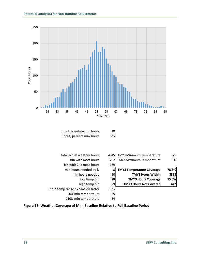
The best approach is dependent on the weather coverage available in the different mini periods. In this case, since each mini period is 6 months, neither one provides great weather coverage. ECAM now provides a calculation of weather coverage. Usually a weather coverage calculation compares the actual temperatures available to the hours at each temperature in a typical year. In this case, however, the comparison is to how well each mini period covers the full range of actual temperatures in the full year.

Figures 13 and 14 show the weather coverage for the baseline and post mini periods respectively.



Figure 13. Weather Coverage of Mini Baseline Relative to Full Baseline Period

input, absolute min hours 10

input, percent max hours 2%

total actual weather hours 4345 TMY3 Minimum Temperature 25

bin with most hours 207 TMY3 Maximum Temperature 100

bin with 2nd most hours 189

min hours needed by % 8 TMY3 Temperature Coverage 78.6%

min hours needed 10 TMY3 Hours Within 8318

low temp bin 28 TMY3 Hours Coverage 95.0%

high temp bin 79 TMY3 Hours Not Covered 442

input temp range expansion factor 10%

90% min temperature 25


0

50

100

150

200

250

88837873686358534843383328

To

tal

Ho

urs

1degBin



Figure 14. Weather Coverage of Mini Post Period Relative to Full Baseline Period

input, absolute min hours 10

input, percent max hours 2%

total actual weather hours 4417 TMY3 Minimum Temperature 25

bin with most hours 259 TMY3 Maximum Temperature 100

bin with 2nd most hours 227

min hours needed by % 10 TMY3 Temperature Coverage 72.9%

min hours needed 10 TMY3 Hours Within 7756

low temp bin 50 TMY3 Hours Coverage 88.5%

high temp bin 96 TMY3 Hours Not Covered 1004

input temp range expansion factor 10%



0

50

100

150

200

250

300

10197938985817773696561575349

To

tal

Ho

urs

1degBin



The temperature coverage in the mini baseline period covers the temperatures in the full baseline period for over 95% of the hours in the full baseline period. That is pretty good, and much better than the coverage provided by the mini post period.

Therefore, we can reasonably estimate the impact of the change using a normal forecast model, using the mini baseline and mini post and estimating avoided energy use:

426,018 Adjusted Baseline Energy

436,175 Measured Energy

-10,157 Avoided Energy Use

The estimated impact of the permanent schedule change, based on a model for the mini baseline time period, is an increase in energy use of 10,157 kWh for the 6 month period after the schedule increase (the mini post period.)

This method incorporates the weather and time-related aspects of the change, subject to the adequacy of the weather coverage.

4.2.2.3. A Simple Pre-Post Approach Using a Forecast Model

For situations where the weather coverage is inadequate in both the mini baseline and mini post periods, a pre-post approach that includes all the data can be employed. This example uses a simple pre-post model with two coefficients to represent the average impact of the schedule change for the two hours of the day that are affected.

This is the approach described in Section 3.2.1.2. In this example, the fundamental change in energy use for the two affected hours of the day was a constant, except it also depended on the outside air temperatures in those hours. Recall that the assumption here was that there was no weather-dependent electricity use during unoccupied hours, but the electricity use during occupied hours was weather dependent. Hence, this changed schedule actually has some weather dependency. Since, at the end of the day, temperatures tend to be going down, including separate coefficients for each of the two affected hours will provide some incorporation of the effect of temperatures.

With a true pre-post model, the least squares fit would be found in one step. With a forecast model, and models that may have change points, this is an iterative process. The initial estimate can be made with values of 0 for the coefficients for the schedule change. After each trial, the error in the modeled electricity use for each affected hour (e.g. hours 18 and 19 of all days) can be estimated. Then the slope for the change in the error divided by the change in the coefficient can be estimated, and new coefficients tried. The table below shows the iterative process:



The estimated impact of the permanent schedule change, based on a simple pre-post model with 2 coefficients, one for each affected hour, is an increase in energy use of 9,660 kWh for the 6 month period after the schedule increase.

Coefficient for kW adjustment at hour 18 0 25 31.2 30.9 30.9

Coefficient for kW adjustment at hour 19 0 20 21.1 22.3 21.6

NR Event Period Adjustment 0 8,280 9,623 9,789 9,660

RMSE 9.37 7.79 7.74 7.74 7.74

R2 0.718 0.804 0.808 0.809 0.809

Hour 18 NR Event Error 4,809 961 -57 13 1

Hour 19 NR Event Error 3,093 166 86 -120 -3

Total NR Event Error, affected hours 7,902 1,128 29 -107 -1

a a ay a - bpa.gov

Documents