a flamelet approach for the simulation of swirling
TRANSCRIPT
Facolta di Ingegneria Civile e Industriale
Dipartimento di Ingegneria Meccanica e Aerospaziale
A flamelet approach for the simulation ofswirling turbulent non-premixed flames
THESIS ADVISOR: AUTHOR:
Prof. Francesco Creta Sebastian Sanchez Riera
CO-ADVISORS:
Dr. Pasquale Lapenna
Dr. Giuseppe Indelicato
Dr. Rachele Lamioni
Academic Year 2018/2019

Acknowledgements
Este Trabajo Final de Grado supone la culminacion a cuatro anos de esfuerzo y trabajoduro. Por ello, me gustarıa aprovechar esta oportunidad para dar las gracias a todos aquellosque me han acompanado durante este tiempo, especialmente mis padres y hermano.
Agradecer tambien a la Universitat Politecnica de Valencia y a la Escuela Tecnica Superiorde Ingenierıa del Diseno por darme la oportunidad de cursar el Grado en IngenierıaAeroespacial, ası como a su profesorado.
Otra parte fundamental en todo este camino han sido los companeros de la universidad,con quienes he tenido el placer de emprender, compartir y finalizar esta aventura.
Por ultimo, pero no por ello menos importante, agradezco especialmente al Prof. FrancescoCreta junto a Dr. Pasquale Lapenna, Dr. Giuseppe Indelicato y Dr. Raquele Lamioni porbrindarme la oportunidad de trabajar en este Trabajo Final de Grado, depositando ası toda suconfianza en mı.
GRACIAS
Aquest Treball Final de Grau suposa la culminacio a quatre anys d’esforc i treball dur. Peraixo, m’agradaria aprofitar aquesta ocasio per a donar les gracies a tots aquells que m’hanacompanyat al llarg d’aquest temps, especialment els meus pares i germa.
Agrair tambe a la Universitat Politecnica de Valencia i a l’Escola Tecnica Superiord’Enginyeria del Disseny per brindar-me l’oportunitat de cursar el Grau en EnginyeriaAeroespacial, aixı com al professorat.
Una altra part fonamental en tot aquest camı han sigut els companys de la universitat, ambqui he tingut el plaer d’emprendre, compartir i finalitzar aquesta aventura.
Per ultim, pero no per aixo menys important, agraısc especialment al Prof. Francesco Cretajunt amb Dr. Pasquale Lapenna, Dr. Giuseppe Indelicato i Dr. Raquele Lamioni per brindar-mel’oportunitat de treballar en aquest Treball Final de Grau, depositant aixı tota la seua confiancaen mi.
GRACIES
I

ACKNOWLEDGEMENTS
II
Abstract
Aerospace industry and its continuous seek for technological improvements are responsiblefor the innovations experienced during the last decades. In this sense, swirling flamesconstitute a point of interest for the combustion field, and its study is what has motivatedthis thesis project. In particular, the main objective of this work is to implement a swirlingflow in OpenFOAM environment by setting a new boundary condition, named swirl. Then,both non-reactive and reactive flow simulations are carried out, whose analysis is done bycomparing and validating them with experimental data.
Focusing onto the reactive case (swirling non-premixed flame), the methodology usedis based on Computational Fluid Dynamics techniques which allow solving turbulentcombustion problems through the implementation of a numerical approach known asFlamelet approach. It consists on decoupling the combustion process into two subsets: mixingand flame structure. This method is attainable thanks to the introduction of a passive scalar:the mixture fraction z.
La costante ricerca di miglioramenti tecnologici nell’ambito dell’industria aerospaziale ela principale responsabile delle innovazioni nel settore delle ultime decadi. In questo sensole swirling f lames costituiscono un punto di grande interesse nel mondo della combustione,la volonta di studiarle motiva la realizzazione di questa tesi. Nello specifico, l’obiettivo dellavoro riguarda l’implementazione di uno swirling f low nell’ambiente di lavoro OpenFOAMattraverso la creazione di una nuova condizione di contorno chiamata swirl. Oltre a ciosono effettuate sia simulazioni del flusso non reattivo che del flusso reattivo, queste sono poianalizzate e validate tramite il confronto dei risultati con dati sperimentali.
Concentrandosi sul caso del flusso reattivo (swirling non− premixed f lame), la metodologiausata e basata sulle tecniche della Meccanica dei Fluidi Computazionale, le quali permettonodi risolvere problemi di combustione turbolenta mediante l’uso di un approccio numericochiamato Flamelet approach. Questo permette di disaccoppiare il processo di combustionein due parti: mescolamento e struttura della fiamma. Tale metodo e possibile grazieall’introduzione di uno scalare passivo: la frazione di miscela z.
III
ABSTRACT
La industria aeroespacial junto a su continua busqueda de mejoras a nivel tecnologicoson las principales responsables de las innovaciones experimentadas en el sector durante lasultimas decadas. En esta lınea, las swirling f lames constituyen un punto de gran interes enel campo de la combustion, y su estudio es lo que ha motivado la realizacion de esta TrabajoFinal de Grado. Especıficamente, el objetivo de este proyecto es implementar un swirlingf low en el ambiente de trabajo OpenFOAM a traves de la creacion de una nueva condicion decontorno, llamada swirl. A continuacion, tanto las simulaciones de flujo no reactivo como deflujo reactivo son llevadas a cabo, cuyo analisis consiste en la comparacion y validacion de losresultados con datos experimentales.
Centrandonos en el caso del flujo reactivo (swirling non− premixed f lame), la metodologıausada se basa en las tecnicas de la Mecanica de Fluidos Computacional, las cuales permitenresolver problemas de combustion turbulenta mediante el uso de un enfoque numericollamado Flamelet approach. Este permite desacoplar el proceso de combustion en dos partes:mezclado y estructura de la llama. Este metodo es posible gracias a la introduccion de unescalar pasivo: la fraccion de mezcla z.
La industria aeroespacial i la seua continua recerca de millores a nivell tecnologic son lesprincipals responsables de les innovacions experimentades en el sector durant les ultimesdecades. En esta lınia, les swirling f lames constituıxen un punt de gran interes en el camp dela combustio, i el seu estudi es el que ha motivat la realitzacio d’aquest Treball Final de Grau.De manera especıfica, l’objectiu d’aquest projecte es la implementacio d’una nova condiciode contorno, denominada swirl. A continuacio, tant les simulacions de fluxos no reactiuscom reactius son dutes a terme, l’analisi de les quals es basa en la comparacio i validacio delsresultats amb dades experimentals.
Centrant-se en el cas del flux reactiu (swirling non− premixed f lame), la metodologia usadaes troba basada en les tecniques de la Mecanica de Fluids Computacional, les quals permetenresoldre problemes de combustio turbulenta mitjancant l’us d’un enfocament numeric nomenatFlamelet approach. Aquest permet desacoblar el proces de combustio en dues parts: mesclat iestructura de la flama. Aquest metode es possible gracies a la introduccio d’un escalar passiu:la fraccio de mescla z.
IV
Key words
Swirling non-premixed flames
Turbulent combustion
Flamelet approach
OpenFOAM environment
V

KEY WORDS
VI
Contents
Acknowledgements I
Abstract III
Key words V
List of Figures IX
List of Tables XI
Nomenclature XIII
1 Introduction 11.1 Motivation . . . . . . . . . . . . . . . . . . . . . . . . . . . . . . . . . . . . . . . . . 11.2 Objectives . . . . . . . . . . . . . . . . . . . . . . . . . . . . . . . . . . . . . . . . . 1
2 Theoretical framework 32.1 Introduction to combustion . . . . . . . . . . . . . . . . . . . . . . . . . . . . . . . 32.2 Laminar diffusion flames . . . . . . . . . . . . . . . . . . . . . . . . . . . . . . . . . 4
2.2.1 Main characteristics . . . . . . . . . . . . . . . . . . . . . . . . . . . . . . . 42.2.2 Governing equations . . . . . . . . . . . . . . . . . . . . . . . . . . . . . . . 52.2.3 Passive scalars and mixture fraction . . . . . . . . . . . . . . . . . . . . . . 72.2.4 Laminar Flamelet Model . . . . . . . . . . . . . . . . . . . . . . . . . . . . . 92.2.5 Diffusion flame structures . . . . . . . . . . . . . . . . . . . . . . . . . . . . 11
2.3 Introduction to turbulent combustion . . . . . . . . . . . . . . . . . . . . . . . . . 142.3.1 Turbulent flows . . . . . . . . . . . . . . . . . . . . . . . . . . . . . . . . . . 152.3.2 Interaction between combustion and turbulence . . . . . . . . . . . . . . . 162.3.3 Computational approaches for turbulent combustion . . . . . . . . . . . . 16
2.4 Turbulent non-premixed flames . . . . . . . . . . . . . . . . . . . . . . . . . . . . . 212.4.1 Main characteristics . . . . . . . . . . . . . . . . . . . . . . . . . . . . . . . 212.4.2 Turbulent Flamelet Model . . . . . . . . . . . . . . . . . . . . . . . . . . . . 23
2.5 Swirling flames . . . . . . . . . . . . . . . . . . . . . . . . . . . . . . . . . . . . . . 292.5.1 Introduction to swirling flows . . . . . . . . . . . . . . . . . . . . . . . . . 292.5.2 Applications in the combustion field . . . . . . . . . . . . . . . . . . . . . . 34
3 Methodology 373.1 Computational Fluid Dynamics . . . . . . . . . . . . . . . . . . . . . . . . . . . . . 37
3.1.1 OpenFOAM environment . . . . . . . . . . . . . . . . . . . . . . . . . . . . 393.2 Swirl boundary condition . . . . . . . . . . . . . . . . . . . . . . . . . . . . . . . . 40
3.2.1 OpenFOAM code . . . . . . . . . . . . . . . . . . . . . . . . . . . . . . . . . 40
VII
CONTENTS
3.2.2 Turbulence model selection . . . . . . . . . . . . . . . . . . . . . . . . . . . 41
4 Numerical results 434.1 Validation of the swirl boundary condition . . . . . . . . . . . . . . . . . . . . . . 43
4.1.1 Non-reactive flow . . . . . . . . . . . . . . . . . . . . . . . . . . . . . . . . . 434.1.2 Non-reactive flow by flamelet model . . . . . . . . . . . . . . . . . . . . . . 494.1.3 Reactive flow . . . . . . . . . . . . . . . . . . . . . . . . . . . . . . . . . . . 51
5 Conclusions 69
6 Prospective research 71
7 Bibliography 73
VIII
List of Figures
2.1 Laminar diffusion flames - Flame structure . . . . . . . . . . . . . . . . . . . . . . 42.2 Laminar diffusion flames - Stretched flame . . . . . . . . . . . . . . . . . . . . . . 52.3 Laminar diffusion flames - Problem decoupling . . . . . . . . . . . . . . . . . . . 112.4 Laminar diffusion flames - Burke-Schumann solution for fast and irreversible
reactions . . . . . . . . . . . . . . . . . . . . . . . . . . . . . . . . . . . . . . . . . . 122.5 Laminar diffusive flames - Chemistry processes . . . . . . . . . . . . . . . . . . . 132.6 Laminar diffusion flames - Burke-Schumann solution for fast and irreversible
reactions . . . . . . . . . . . . . . . . . . . . . . . . . . . . . . . . . . . . . . . . . . 142.7 Introduction to turbulent combustion - Energy Cascade . . . . . . . . . . . . . . . 162.8 Introduction to turbulent combustion - Turbulence models over energy spectrum 172.9 Turbulent non-premixed flames - Fuel jet discharging in ambient air . . . . . . . 212.10 Turbulent non-premixed flames - Flame stabilization using bluff-body . . . . . . 222.11 Turbulent non-premixed flames - Combustion diagram . . . . . . . . . . . . . . . 232.12 Turbulent non-premixed flames - Diffusion flame structure ambiguity . . . . . . 262.13 Turbulent non-premixed flames - pd f functions . . . . . . . . . . . . . . . . . . . . 272.14 Turbulent non-premixed flames - Primitive variables approach . . . . . . . . . . . 282.15 Introduction to swirling flows - Velocity components . . . . . . . . . . . . . . . . 292.16 Introduction to swirling flows - Velocity fluctuations . . . . . . . . . . . . . . . . . 302.17 Introduction to swirling flows - Water tank analogy . . . . . . . . . . . . . . . . . 322.18 Introduction to swirling flows - Tangential velocity profile . . . . . . . . . . . . . 332.19 Swirling flames - Blades configuration for a swirl injector . . . . . . . . . . . . . . 342.20 Swirling flames - Vortex breakdown and preprocessing vortex core . . . . . . . . 36
3.1 Computational Fluid Dynamics - Simulation process . . . . . . . . . . . . . . . . 383.2 Computational Fluid Dynamics - OpenFOAM framework . . . . . . . . . . . . . 40
4.1 Non-reactive flow - 2D axisymmetric geometry . . . . . . . . . . . . . . . . . . . . 444.2 Non-reactive flow - Mesh independence for velocity magnitude . . . . . . . . . . 464.3 Non-reactive flow - Mesh independence for axial velocity . . . . . . . . . . . . . . 474.4 Non-reactive flow - Validation for axial velocity . . . . . . . . . . . . . . . . . . . 484.5 Non-reactive flow - Solvers comparison for axial velocity . . . . . . . . . . . . . . 504.6 Non-reactive flow - Solvers comparison for velocity magnitude . . . . . . . . . . 514.7 Reactive flow - Sydney burner geometry . . . . . . . . . . . . . . . . . . . . . . . . 524.8 Reactive flow - Equivalent pipe . . . . . . . . . . . . . . . . . . . . . . . . . . . . . 534.9 Reactive flow - Loop initial flame conditions . . . . . . . . . . . . . . . . . . . . . 544.10 Reactive flow - Sydney burner computational domain . . . . . . . . . . . . . . . . 554.11 Reactive flow - SM1 mesh independence for axial velocity . . . . . . . . . . . . . 574.12 Reactive flow - SM1 mesh independence for temperature . . . . . . . . . . . . . . 584.13 Reactive flow - SM1 mesh independence for mixture fraction . . . . . . . . . . . . 59
IX

LIST OF FIGURES
4.14 Reactive flow - SM1 axial velocity . . . . . . . . . . . . . . . . . . . . . . . . . . . . 604.15 Reactive flow - SM1 temperature . . . . . . . . . . . . . . . . . . . . . . . . . . . . 614.16 Reactive flow - SM1 mixture fraction . . . . . . . . . . . . . . . . . . . . . . . . . . 624.17 Reactive flow - SM1 temperature field comparison . . . . . . . . . . . . . . . . . . 664.18 Reactive flow - SM1 mixture fraction field . . . . . . . . . . . . . . . . . . . . . . . 664.19 Reactive flow - SM1 axial velocity field . . . . . . . . . . . . . . . . . . . . . . . . . 67
X
List of Tables
2.1 Laminar diffusion flames - Chemistry mechanism . . . . . . . . . . . . . . . . . . 132.2 Introduction to turbulent combustion - Turbulence models . . . . . . . . . . . . . 202.3 Turbulent non-premixed flames - Laminar and turbulent flamelet models . . . . 242.4 Turbulent non-premixed flames - Principle of a pd f flamelet model using
primitive variables . . . . . . . . . . . . . . . . . . . . . . . . . . . . . . . . . . . . 28
4.1 Non-reactive flow - Mesh properties . . . . . . . . . . . . . . . . . . . . . . . . . . 464.2 Reactive flow - SM1 flame properties . . . . . . . . . . . . . . . . . . . . . . . . . . 534.3 Reactive flow - SM1 flame initial conditions . . . . . . . . . . . . . . . . . . . . . . 544.4 Reactive flow - SM1 mesh properties . . . . . . . . . . . . . . . . . . . . . . . . . . 56
XI

LIST OF TABLES
XII
Nomenclature
Abbreviations
Cp — Constant pressure heat capacity [J/(K · kg)]D — Pipe diameter [m]Deq — Equivalent pipe diameter [m]Di — Internal pipe diameter [m]Dk — Molecular diffusivity of the k-th species [mol/m3]Do — Outer pipe diameter [m]Da — Damkohler number [-]Daig — Ignition Damkohler number [-]Daq — Quenching Damkohler number [-]fm — Body forces [m/s2]hs — Sensible enthalpy [J/kg]K(T) — Equilibrium constant [-]k — Turbulent kinetic energy [J/kg]L0 — Integral turbulence scale [m]Le — Lewis number [-]p — Pressure [Pa]Q — Heat source per unit volume [J/(m3 · s)]R — Air ideal gas constant [J/(kg · K)]Re — Reynolds number [-]r — Radial coordinate [m]S — Swirl number [-]Sg — Geometric Swirl number [-]T — Temperature [K]t — Time [s]tc — Chemical time scale [s]t f — Flow time scale [s]U — Mean axial velocity [m/s]u — Axial velocity [m/s]u′ — Fluctuating axial velocity [m/s]V — Mean radial velocity [m/s]Vk — Diffusion velocity of k-th species [m/s]v — Radial velocity [m/s]v′ — Fluctuating radial velocity [m/s]v — Velocity vector [m/s]W — Mean tangential velocity [m/s]w — Tangential velocity [m/s]w′ — Fluctuating tangential velocity [m/s]
XIII
NOMENCLATURE
x — Longitudinal coordinate [m]Y — Mass fraction [-]Z — Passive scalar [-]z — Mixture fraction [-]
Greek letters
ε — Eddy dissipation rate [m2/s3]λ — Thermal conductivity [W/(m · K)]µ — Kinematic viscosity [Pa · s]ν — Dynamic viscosity [m2/s]ω — Angular velocity [rad/s]ωk — Mass reaction rate of k-th species [kg/s ·m3]ω′T — Thermal reaction rate [J/(m3 · s)]ρ — Density [kg/m3]σ — Stress [Pa]τij — Viscous stress tensor [Pa]ϕ — Azimuthal angle [o]χ — Scalar dissipation [1/s]χst — Stoichiometric scalar dissipation [1/s]
Acronyms
CFD — Computational Fluid DynamicsDNS — Direct Numerical SimulationsFVM — Finite Volume MethodLES — Large Eddy Simulationspdf — Probability density functionPVC — Precessing Vortex CoreRANS— Reynolds Averaged Navier-StokesSRS — Scale Resolving SimulationsVB — Vortex Breakdown
XIV
Chapter 1
Introduction
1.1 Motivation
For recent years, the use of swirling flows has become a common trend in a wide range ofapplications. The development experienced by the aerospace industry, which is continuouslyseeking for better performances while reducing costs, has motivated the introduction ofswirling flows in an innovative way. Turbomachinery, large pipeline systems or combustionchambers are some good examples. In the past decades, most of the studies were focused oninternal swirling flows, particularly flow in pipes, but recent investigations are pointing into anew direction, which is swirl injectors. During the development of this thesis, we will focus onthis last application.
In this sense, swirling flames constitute a point of interest for the combustion field. Theyoffer a wide range of advantages such as flame stabilization, reduction of unburned gasesand mixing enhancement. These features are due to the creation of a recirculation bubble,which is related to a complex flow structure derived from the swirl motion. It is the socalled Vortex Breakdown (VB) and it constitutes the dominant flame stabilisation mechanismthanks to its characteristic reverse flows (recirculation). This structure can eventually developinto a Precessing Vortex Core (PVC), whose oscillation contributes to the improvement incombustion efficiency and mixing.
1.2 Objectives
The main objective of this thesis project is to implement a swirling flow in OpenFOAMenvironment by setting a new boundary condition, named swirl. Once it is achieved,an intensive validation process is carried out by simulating both non reactive and reactiveflow well known cases. In this way, the numerical results are compared with experimental data.
Focusing onto the reactive case (swirling flame), the methodology used is basedon Computational Fluid Dynamics techniques which allow solving turbulent combustionproblems through the implementation of a numerical approach known as Flamelet approach.It consists on decoupling the combustion process into two subsets: mixing and flame structure.This method is attainable thanks to the introduction of a passive scalar: the mixture fractionz. The solver used is flameletPimpleSMOKE, which is a solver belonging to Dipartamento diIngegneria Meccanica e Aerospaziale of Sapienza University of Rome.
1
CHAPTER 1. INTRODUCTION
Regarding the simulations, Realizable k− ε (RANS) model is used for turbulence modellingdue to its reduced computational cost. As a consequence, the suitability of this model will bealso analysed.
So, to sum up, the objectives of the present work are to introduce a swirl motion inOpenFOAM environment as well as, to analyse the requirements imposed by swirling flamesin terms of turbulence modelling.
2
Chapter 2
Theoretical framework
The aim of this chapter is to set the theoretical basics needed to develop this thesis project.As starting point, a brief comment about combustion is done in order to introduce the maingeneral concepts and the different types of combustion. After that, the focus is pointedinto non-premixed flames, whose study through computational fluid dynamics techniquesconstitutes our scope.
To fully describe non-premixed flames, laminar diffusion flames are explained beforemoving to the turbulent ones. A fundamental part of this chapter is given by the descriptionand characterization of the computational approach used, which is based on the flameletassumption.
Finally, swirling flames are explained by characterising a swirling flow as well asintroducing its applications in the combustion field.
2.1 Introduction to combustion
A commonly extended academic definition of combustion is: ” Combustion is a hightemperature exothermic redox (reduction-oxidation) chemical reaction between a fuel (thereductant which is oxidized) and an oxidizer (which is reduced), usually atmospheric oxygen ”.
A more useful definition is: ” Combustion is the rearrangement of atoms and, thus, ofchemical covalent bonds between reactants and products ” . It means that nuclear reactions arenot involving a combustion process, since atoms are changed. However, chemical reactions,which may involve a combustion process if a fuel and oxidizer are present, only rearrange theatoms (elements) to form new molecules (species), i.e. atoms are conserved. Then, combustioninvolves two process: chemical reactions with its consequent production of heat and theconvective/diffusive transport of heat and molecules. [1]
One forward step can be done by introducing the two types of combustion. They can beclassified into: [2]
− Premixed combustion: It is characterised by the presence of a combustable mixture offuel and oxidizer. Once ignition occurs, the resulting premixed flame tends to act asa sink for reactants and a source of products. Thus, it will tend to propagate into theunburned mixture. Then, premixed combustion is a wave phenomenon that impliespropagation. Depending on the velocity of the combustion wave, premixed combustion
3
CHAPTER 2. THEORETICAL FRAMEWORK
can be classified into deflagrations (flames) and detonations. While flames are subsonicand controlled, detonations are subsonic and uncontrolled.
− Non-premixed (diffusive) combustion: It is a typical flame for most combustion systemswhere fuel and oxidizer are initially separated. For example, a coaxial burner having acentral fuel nozzle and an outer oxidizer nozzle will give rise to a non-premixed flame.This is the case studied in this thesis project. In addition, candle flame and dropletcombustion also constitute good examples of non-premixed combustion.
2.2 Laminar diffusion flames
Diffusion flames constitute a specific class of combustion problems where fuel and oxidizerare not mixed before they enter the combustion chamber: for these flames, mixing must bringreactants into reaction zone fast enough for combustion to proceed. Then, mixing becomes oneof the main issues in diffusion flames.
2.2.1 Main characteristics
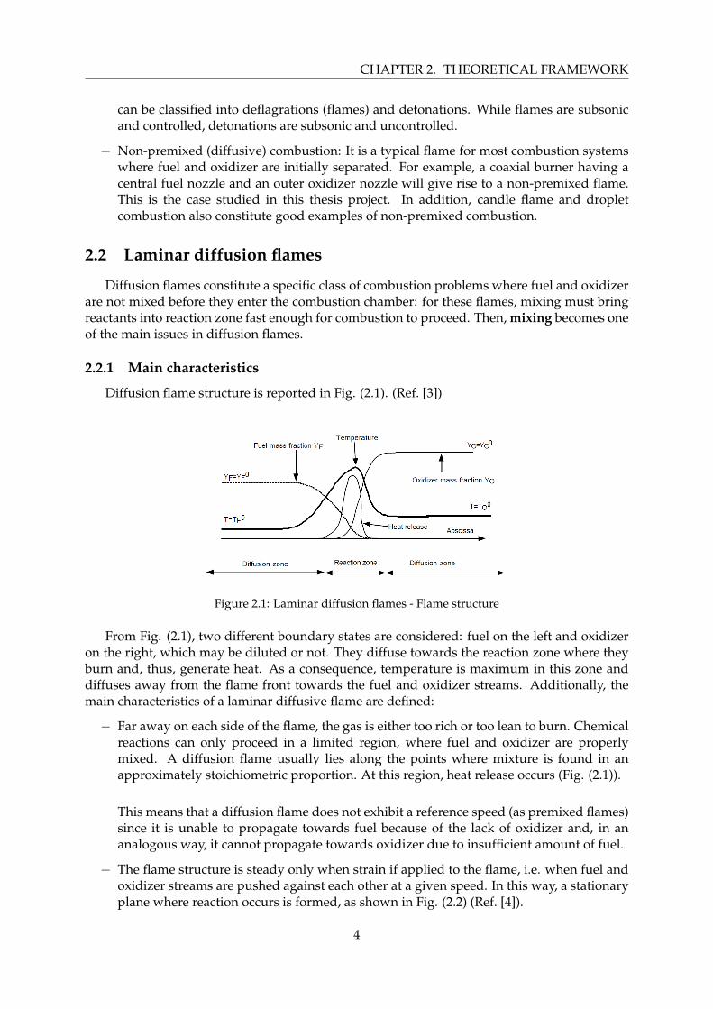
Diffusion flame structure is reported in Fig. (2.1). (Ref. [3])
Figure 2.1: Laminar diffusion flames - Flame structure
From Fig. (2.1), two different boundary states are considered: fuel on the left and oxidizeron the right, which may be diluted or not. They diffuse towards the reaction zone where theyburn and, thus, generate heat. As a consequence, temperature is maximum in this zone anddiffuses away from the flame front towards the fuel and oxidizer streams. Additionally, themain characteristics of a laminar diffusive flame are defined:
− Far away on each side of the flame, the gas is either too rich or too lean to burn. Chemicalreactions can only proceed in a limited region, where fuel and oxidizer are properlymixed. A diffusion flame usually lies along the points where mixture is found in anapproximately stoichiometric proportion. At this region, heat release occurs (Fig. (2.1)).
This means that a diffusion flame does not exhibit a reference speed (as premixed flames)since it is unable to propagate towards fuel because of the lack of oxidizer and, in ananalogous way, it cannot propagate towards oxidizer due to insufficient amount of fuel.
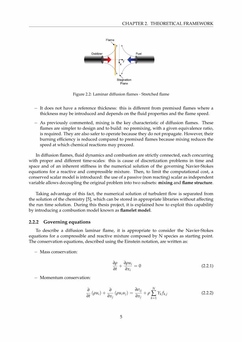
− The flame structure is steady only when strain if applied to the flame, i.e. when fuel andoxidizer streams are pushed against each other at a given speed. In this way, a stationaryplane where reaction occurs is formed, as shown in Fig. (2.2) (Ref. [4]).
4
CHAPTER 2. THEORETICAL FRAMEWORK
Figure 2.2: Laminar diffusion flames - Stretched flame
− It does not have a reference thickness: this is different from premixed flames where athickness may be introduced and depends on the fluid properties and the flame speed.
− As previously commented, mixing is the key characteristic of diffusion flames. Theseflames are simpler to design and to build: no premixing, with a given equivalence ratio,is required. They are also safer to operate because they do not propagate. However, theirburning efficiency is reduced compared to premixed flames because mixing reduces thespeed at which chemical reactions may proceed.
In diffusion flames, fluid dynamics and combustion are strictly connected, each concurringwith proper and different time-scales: this is cause of discretization problems in time andspace and of an inherent stiffness in the numerical solution of the governing Navier-Stokesequations for a reactive and compressible mixture. Then, to limit the computational cost, aconserved scalar model is introduced: the use of a passive (non reacting) scalar as independentvariable allows decoupling the original problem into two subsets: mixing and flame structure.
Taking advantage of this fact, the numerical solution of turbulent flow is separated fromthe solution of the chemistry [5], which can be stored in appropriate libraries without affectingthe run time solution. During this thesis project, it is explained how to exploit this capabilityby introducing a combustion model known as flamelet model.
2.2.2 Governing equations
To describe a diffusion laminar flame, it is appropriate to consider the Navier-Stokesequations for a compressible and reactive mixture composed by N species as starting point.The conservation equations, described using the Einstein notation, are written as:
− Mass conservation:
∂ρ
∂t+
∂ρui
∂xi= 0 (2.2.1)
− Momentum conservation:
∂
∂t(ρui) +
∂
∂xj(ρuiuj) =
∂σij
∂xj+ ρ
N
∑k=1
Yk fk,j (2.2.2)
5
CHAPTER 2. THEORETICAL FRAMEWORK
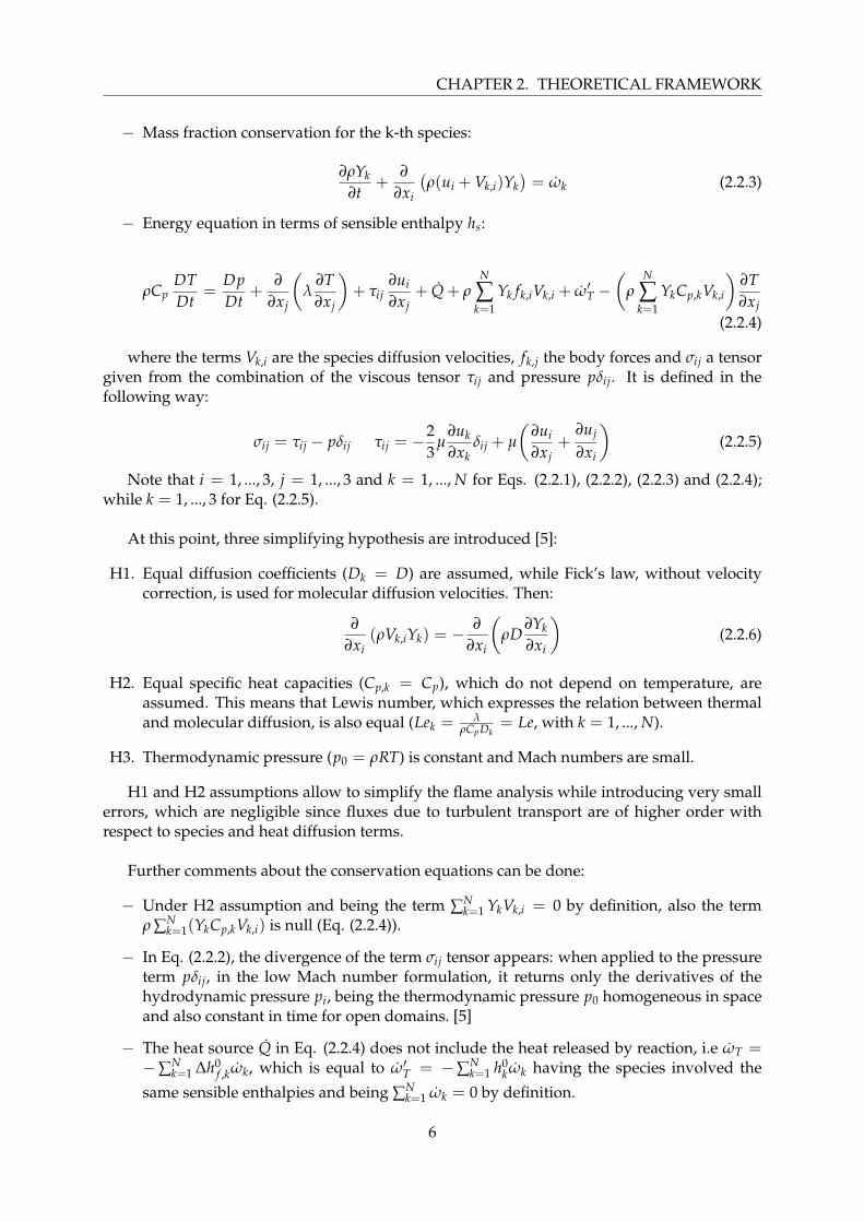
− Mass fraction conservation for the k-th species:
∂ρYk
∂t+
∂
∂xi
(ρ(ui + Vk,i)Yk
)= ωk (2.2.3)
− Energy equation in terms of sensible enthalpy hs:
ρCpDTDt
=DpDt
+∂
∂xj
(λ
∂T∂xj
)+ τij
∂ui
∂xj+ Q + ρ
N
∑k=1
Yk fk,iVk,i + ω′T −(
ρN
∑k=1
YkCp,kVk,i
)∂T∂xj
(2.2.4)
where the terms Vk,i are the species diffusion velocities, fk,j the body forces and σij a tensorgiven from the combination of the viscous tensor τij and pressure pδij. It is defined in thefollowing way:
σij = τij − pδij τij = −23
µ∂uk
∂xkδij + µ
(∂ui
∂xj+
∂uj
∂xi
)(2.2.5)
Note that i = 1, ..., 3, j = 1, ..., 3 and k = 1, ..., N for Eqs. (2.2.1), (2.2.2), (2.2.3) and (2.2.4);while k = 1, ..., 3 for Eq. (2.2.5).
At this point, three simplifying hypothesis are introduced [5]:
H1. Equal diffusion coefficients (Dk = D) are assumed, while Fick’s law, without velocitycorrection, is used for molecular diffusion velocities. Then:
∂
∂xi(ρVk,iYk) = −
∂
∂xi
(ρD
∂Yk
∂xi
)(2.2.6)
H2. Equal specific heat capacities (Cp,k = Cp), which do not depend on temperature, areassumed. This means that Lewis number, which expresses the relation between thermaland molecular diffusion, is also equal (Lek =
λρCpDk
= Le, with k = 1, ..., N).
H3. Thermodynamic pressure (p0 = ρRT) is constant and Mach numbers are small.
H1 and H2 assumptions allow to simplify the flame analysis while introducing very smallerrors, which are negligible since fluxes due to turbulent transport are of higher order withrespect to species and heat diffusion terms.
Further comments about the conservation equations can be done:
− Under H2 assumption and being the term ∑Nk=1 YkVk,i = 0 by definition, also the term
ρ ∑Nk=1(YkCp,kVk,i) is null (Eq. (2.2.4)).
− In Eq. (2.2.2), the divergence of the term σij tensor appears: when applied to the pressureterm pδij, in the low Mach number formulation, it returns only the derivatives of thehydrodynamic pressure pi, being the thermodynamic pressure p0 homogeneous in spaceand also constant in time for open domains. [5]
− The heat source Q in Eq. (2.2.4) does not include the heat released by reaction, i.e ωT =−∑N
k=1 ∆h0f ,kωk, which is equal to ω′T = −∑N
k=1 h0kωk having the species involved the
same sensible enthalpies and being ∑Nk=1 ωk = 0 by definition.
6
CHAPTER 2. THEORETICAL FRAMEWORK
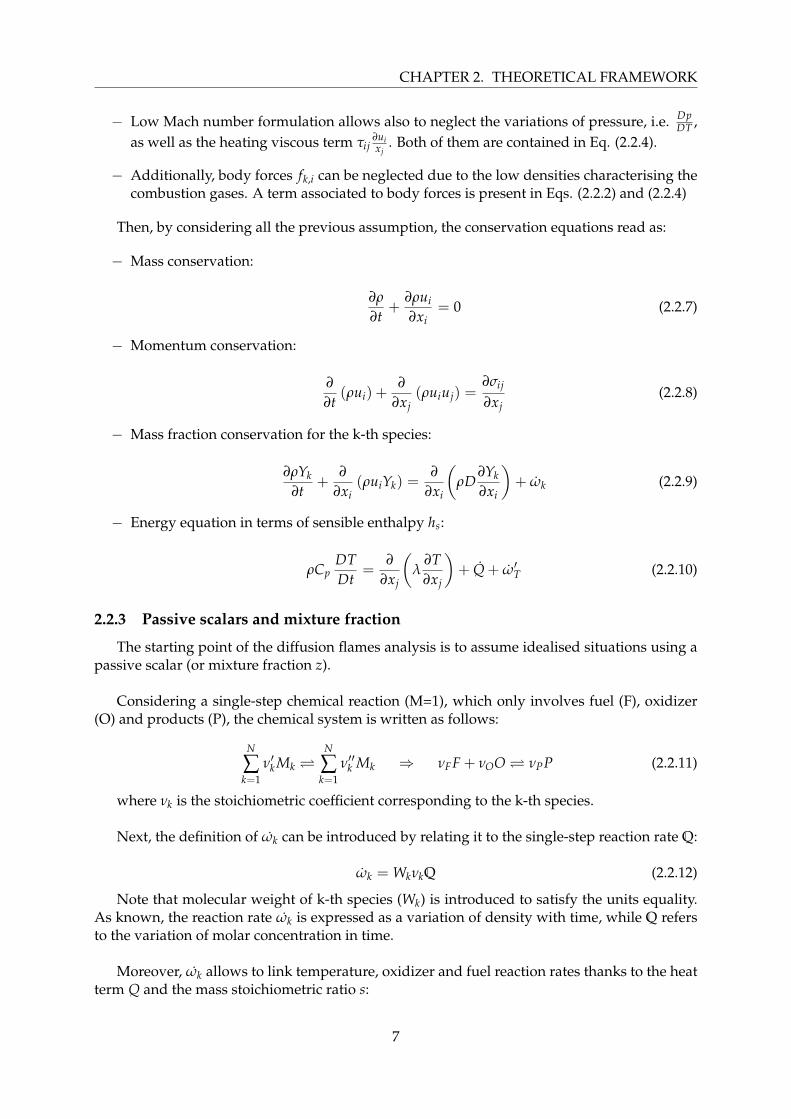
− Low Mach number formulation allows also to neglect the variations of pressure, i.e. DpDT ,
as well as the heating viscous term τij∂uixj
. Both of them are contained in Eq. (2.2.4).
− Additionally, body forces fk,i can be neglected due to the low densities characterising thecombustion gases. A term associated to body forces is present in Eqs. (2.2.2) and (2.2.4)
Then, by considering all the previous assumption, the conservation equations read as:
− Mass conservation:
∂ρ
∂t+
∂ρui
∂xi= 0 (2.2.7)
− Momentum conservation:
∂
∂t(ρui) +
∂
∂xj(ρuiuj) =
∂σij
∂xj(2.2.8)
− Mass fraction conservation for the k-th species:
∂ρYk
∂t+
∂
∂xi(ρuiYk) =
∂
∂xi
(ρD
∂Yk
∂xi
)+ ωk (2.2.9)
− Energy equation in terms of sensible enthalpy hs:
ρCpDTDt
=∂
∂xj
(λ
∂T∂xj
)+ Q + ω′T (2.2.10)
2.2.3 Passive scalars and mixture fraction
The starting point of the diffusion flames analysis is to assume idealised situations using apassive scalar (or mixture fraction z).
Considering a single-step chemical reaction (M=1), which only involves fuel (F), oxidizer(O) and products (P), the chemical system is written as follows:
N
∑k=1
ν′k Mk N
∑k=1
ν′′k Mk ⇒ νFF + νOO νPP (2.2.11)
where νk is the stoichiometric coefficient corresponding to the k-th species.
Next, the definition of ωk can be introduced by relating it to the single-step reaction rate Q:
ωk = WkνkQ (2.2.12)
Note that molecular weight of k-th species (Wk) is introduced to satisfy the units equality.As known, the reaction rate ωk is expressed as a variation of density with time, while Q refersto the variation of molar concentration in time.
Moreover, ωk allows to link temperature, oxidizer and fuel reaction rates thanks to the heatterm Q and the mass stoichiometric ratio s:
7
CHAPTER 2. THEORETICAL FRAMEWORK
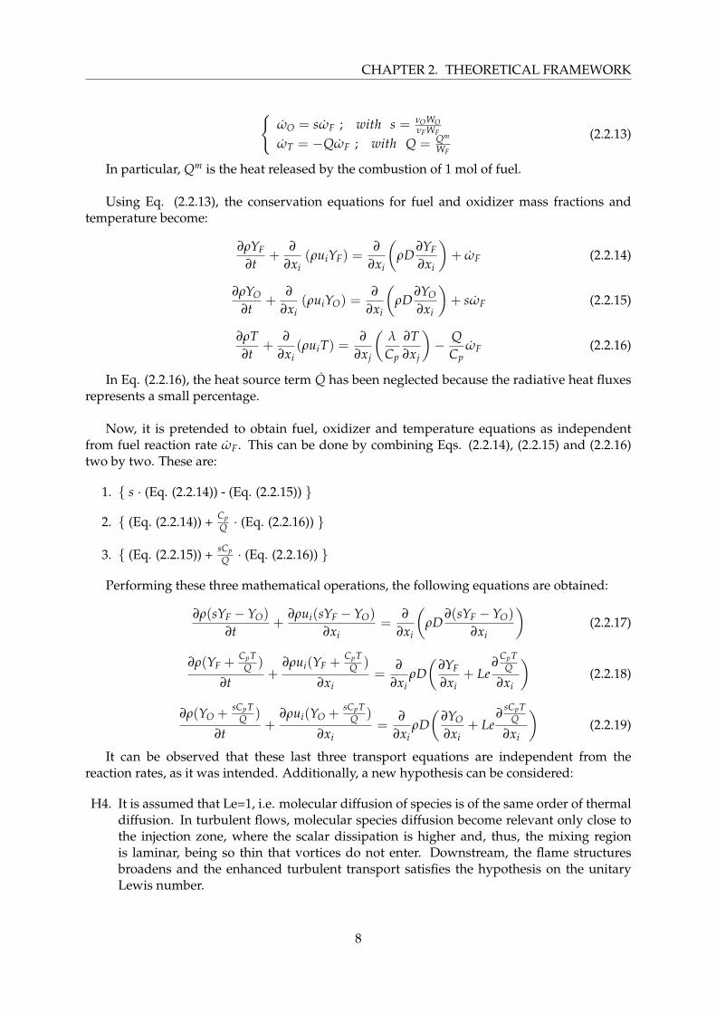
{ωO = sωF ; with s = νOWO
νFWF
ωT = −QωF ; with Q = Qm
WF
(2.2.13)
In particular, Qm is the heat released by the combustion of 1 mol of fuel.
Using Eq. (2.2.13), the conservation equations for fuel and oxidizer mass fractions andtemperature become:
∂ρYF
∂t+
∂
∂xi(ρuiYF) =
∂
∂xi
(ρD
∂YF
∂xi
)+ ωF (2.2.14)
∂ρYO
∂t+
∂
∂xi(ρuiYO) =
∂
∂xi
(ρD
∂YO
∂xi
)+ sωF (2.2.15)
∂ρT∂t
+∂
∂xi(ρuiT) =
∂
∂xj
(λ
Cp
∂T∂xj
)− Q
CpωF (2.2.16)
In Eq. (2.2.16), the heat source term Q has been neglected because the radiative heat fluxesrepresents a small percentage.
Now, it is pretended to obtain fuel, oxidizer and temperature equations as independentfrom fuel reaction rate ωF. This can be done by combining Eqs. (2.2.14), (2.2.15) and (2.2.16)two by two. These are:
1. { s · (Eq. (2.2.14)) - (Eq. (2.2.15)) }
2. { (Eq. (2.2.14)) + CpQ · (Eq. (2.2.16)) }
3. { (Eq. (2.2.15)) + sCpQ · (Eq. (2.2.16)) }
Performing these three mathematical operations, the following equations are obtained:
∂ρ(sYF −YO)
∂t+
∂ρui(sYF −YO)
∂xi=
∂
∂xi
(ρD
∂(sYF −YO)
∂xi
)(2.2.17)
∂ρ(YF +CpT
Q )
∂t+
∂ρui(YF +CpT
Q )
∂xi=
∂
∂xiρD(
∂YF
∂xi+ Le
∂CpT
Q
∂xi
)(2.2.18)
∂ρ(YO +sCpT
Q )
∂t+
∂ρui(YO +sCpT
Q )
∂xi=
∂
∂xiρD(
∂YO
∂xi+ Le
∂sCpT
Q
∂xi
)(2.2.19)
It can be observed that these last three transport equations are independent from thereaction rates, as it was intended. Additionally, a new hypothesis can be considered:
H4. It is assumed that Le=1, i.e. molecular diffusion of species is of the same order of thermaldiffusion. In turbulent flows, molecular species diffusion become relevant only close tothe injection zone, where the scalar dissipation is higher and, thus, the mixing regionis laminar, being so thin that vortices do not enter. Downstream, the flame structuresbroadens and the enhanced turbulent transport satisfies the hypothesis on the unitaryLewis number.
8
CHAPTER 2. THEORETICAL FRAMEWORK
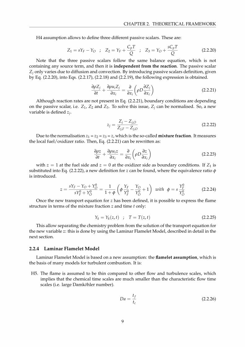
H4 assumption allows to define three different passive scalars. These are:
Z1 = sYF −YO ; Z2 = YF +CpT
Q; Z3 = YO +
sCpTQ
(2.2.20)
Note that the three passive scalars follow the same balance equation, which is notcontaining any source term, and then it is independent from the reaction. The passive scalarZj only varies due to diffusion and convection. By introducing passive scalars definition, givenby Eq. (2.2.20), into Eqs. (2.2.17), (2.2.18) and (2.2.19), the following expression is obtained.
∂ρZj
∂t+
∂ρuiZj
∂xi=
∂
∂xi
(ρD
∂Zj
∂xi
)(2.2.21)
Although reaction rates are not present in Eq. (2.2.21), boundary conditions are dependingon the passive scalar, i.e. Z1, Z2 and Z3. To solve this issue, Zj can be normalised. So, a newvariable is defined zj.
zj =Zj − Zj,O
Zj,F − Zj,O(2.2.22)
Due to the normalisation z1 = z2 = z3 = z, which is the so-called mixture fraction. It measuresthe local fuel/oxidizer ratio. Then, Eq. (2.2.21) can be rewritten as:
∂ρz∂t
+∂ρuiz
∂xi=
∂
∂xi
(ρD
∂z∂xi
)(2.2.23)
with z = 1 at the fuel side and z = 0 at the oxidizer side as boundary conditions. If Z1 issubstituted into Eq. (2.2.22), a new definition for z can be found, where the equivalence ratio φis introduced.
z =sYF −YO + Y0
O
sY0F + Y0
O=
11 + φ
(φ
YF
Y0F− YO
Y0O+ 1)
with φ = sY0
F
Y0O
(2.2.24)
Once the new transport equation for z has been defined, it is possible to express the flamestructure in terms of the mixture fraction z and time t only:
Yk = Yk(z, t) ; T = T(z, t) (2.2.25)
This allow separating the chemistry problem from the solution of the transport equation forthe new variable z: this is done by using the Laminar Flamelet Model, described in detail in thenext section.
2.2.4 Laminar Flamelet Model
Laminar Flamelet Model is based on a new assumption: the flamelet assumption, which isthe basis of many models for turbulent combustion. It is:
H5. The flame is assumed to be thin compared to other flow and turbulence scales, whichimplies that the chemical time scales are much smaller than the characteristic flow timescales (i.e. large Damkohler number).
Da =t f
tc(2.2.26)
9
CHAPTER 2. THEORETICAL FRAMEWORK
This assumption means that, if t f >> tc (flow time scale >> chemical time scale), thereactions happen within times and zones so small that they have no means of interactingwith turbulent phenomena and therefore the flame structure remains laminar. Each elementof the flame front is viewed as a small laminar flame also called f lamelet. Formally, this newassumption is a variable change in the species equation from (x1, x2, x3, t) to (z, y2, y3, t), wherey2, y3 are the spatial variables in planes parallel to the iso-z surfaces. In the resulting equations,terms corresponding to gradients along the flame front, i.e. along y2 and y3, are neglected incomparison to terms normal to the flame, i.e. along z.
On the basis of the flamelet assumption, the structure of the diffusion flame only dependson the mixture fraction z and on time t, as already noted in Eq. (2.2.25). Under this hypothesis,the species mass fractions and temperature balance equations may be rewritten:
ρ∂Yk
∂t= ρD
(∂z∂xi
∂z∂xi
)∂2Yk
∂z2 + ωk (2.2.27)
ρ∂T∂t
= ρD(
∂z∂xi
∂z∂xi
)∂2T∂z2 + ωT (2.2.28)
Now, a new variable is introduced: the Scalar Dissipation χ, which has the dimension of aninverse time [1/s or Hz], like the strain. It measures the gradients of mixture fraction and themolecular fluxes of species towards the flame.
It is directly influenced by the strain: in fact, when the flame strain rate increases, χ alsoincreases. It is defined as:
χ = 2D(
∂z∂xi
∂z∂xi
)(2.2.29)
Once χ is introduced, Eqs. (2.2.27) and (2.2.28) can be expressed as:
ρ∂Yk
∂t=
12
ρχ∂2Yk
∂z2 + ωk (2.2.30)
ρ∂T∂t
=12
ρχ∂2T∂z2 + ωT (2.2.31)
Eqs. (2.2.30) and (2.2.31) are the Flamelet Equations, which are key elements in manydiffusion flame theories. In these equations, the only term depending on spatial variables (xi)is just χ, which controls the mixing. Once χ is specified, the flamelet equations can be entirelysolved in z-space to provide the flame structure, i.e. temperature T and species mass fractionsYk as functions of z and time t.
This means that diffusion flame computations, whose objective is to find T(xi, t) andYk(xi, t), are split into two problems, as initially intended:
− A mixing problem where Eq. (2.2.23) must be solved to obtain the mixture fraction fieldz(xi, t) as a function of spatial coordinates xi and time t.
− A flame structure problem where flame variables are found. They are the species massfractions Yk(z) and temperature T(z), which are solutions of Eqs. (2.2.30) and (2.2.31),respectively.
10
CHAPTER 2. THEORETICAL FRAMEWORK
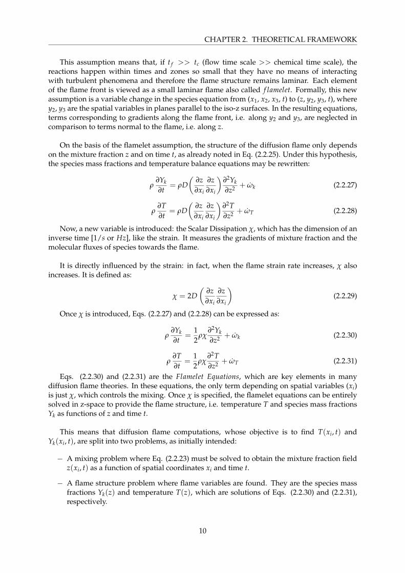
Later, the link between flames variables and z are used to construct all the flame variables(Yk(xi, t) and T(xi, t)). The procedure followed is summarise in Fig. (2.3) (Ref. [3]). Finally, notethat T and Yk are parametrised by the scalar dissipation χ: different values of χ lead to differentflame structures.
Figure 2.3: Laminar diffusion flames - Problem decoupling
2.2.5 Diffusion flame structures
It is possible to predict different diffusion flames structures by doing some assumptions onthe chemistry mechanism, such as:
− Equilibrium condition (Infinitely Fast Chemistry): chemical reactions proceed locally sofast that equilibrium is instantaneously reached. The fast chemistry is controlled by Danumber, which has been already introduced when studying the flamelet laminar model.
− Irreversible condition: chemical reactions only proceed from reactants to products side(unidirectional).
Combining these two assumptions leads to four possible solutions:
· For infinitely fast and irreversible chemistry, fuel and oxidizer cannot coexist at thesame time: once mixing is achieved, the reactants are instantaneously depleted and aninfinitely thin flame separates F and O. This simplest ”equilibrium” assumption is calledirreversible f ast chemistry, in which T(z) and Yk(z) functions are independent from scalardissipation rate.
· For infinitely fast but reversible chemistry, fuel, oxidizer and products mass fractions arelinked by the equilibrium relation (being K(T) the equilibrium constant at temperatureT):
K(T) =YνF
F ·YνOO
YνPP
(2.2.32)
For this case, the flame structure is still independent of the flow condition. In otherwords, scalar dissipation rate χ is not playing any role when infinitely fast chemistryis considered. In particular, χ = 0 for reversible and fast chemistry. In this case, fuel andoxidizer may be found simultaneously at the same location and time.
11
CHAPTER 2. THEORETICAL FRAMEWORK
· For irreversible but not infinitely fast chemistry, fuel and oxidizer may also existsimultaneously, but their concentration now depends on the scalar dissipation rate χ.Temperature and mass fractions must be parametrised by χ.
· For reversible and not infinitely fast chemistry, which is the general case, there are nosimple models to express the dependency of T(z) and Yk(z) on χ.
Further comments can be done for all the equilibrium cases (fast chemestry, i.e. ωk = 0) ifthe steady flamelet equation is considered. It is obtained from Eq. (2.2.30) and it reads as:
ωk = −12
ρχ∂2Yk
∂z2 = 0 (2.2.33)
This equation can be satisfied if: {∂2Yk∂z2 = 0 (1)
χ = 0 (2)(2.2.34)
Relation (1) refers to two different sub-problems:
− A pure mixing problem, where oxidizer and fuel mix without reacting. This process isknown as frozen chemistry.
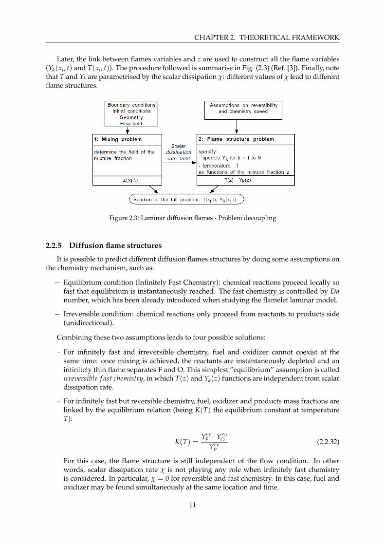
− An infinitely fast chemistry problem for irreversible reactions, where infinitely thinflame separates fuel and oxidizer. In fact, there are not coexisting zones of fuel andoxidizer, being reactants instantaneously depleted once supplied to the reaction zone.This phenomena is reported in Fig. (2.4) (Ref. [3]), which describes Burke-Schumannsolution for the flame structure. [6]
Figure 2.4: Laminar diffusion flames - Burke-Schumann solution for fast and irreversible reactions
12
CHAPTER 2. THEORETICAL FRAMEWORK
On the other hand, relation (2) allows to relax the strong constraint on irreversiblechemistry. Then, it considers the more general context of reversible reactions, for which a fullequilibrium calculation is required. It is governed by Eq. (2.2.32).
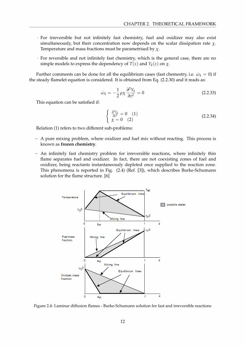
All the described situations are summarised in terms of temperature plots in the z-spacein Fig. (2.5) (Ref. [3]). It can be observed that chemistry effects are only important in thezone where reaction takes place and this zones usually remains small. Outside this region,combustion is zero and the behaviour of the thermofluid properties is independent from thechemistry.
(a) Irreversible fast chemistry (b) Irreversible finite rate chemistry
(c) Reversible fast chemistry (d) Reversible finite rate chemistry
Figure 2.5: Laminar diffusive flames - Chemistry processes
Additionally, the main properties of the chemistry processes described are grouped in Table(2.1).
Chemistry Fast chemistry Finite rate mechanismMechanism (equilibrium): ωk = 0 (non equilibrium): ωk 6= 0
Irreversible F and O cannot coexist F and O may overlap inchemestry (independently of χ) reaction zone (depending on χ)
Reversible F, O and P are in No simple model for thischemestry equilibrium (χ = 0) case (depending on χ)
Frozen F and O mix Not(pure mixing) but do not burn applicable
Table 2.1: Laminar diffusion flames - Chemistry mechanism
13
CHAPTER 2. THEORETICAL FRAMEWORK
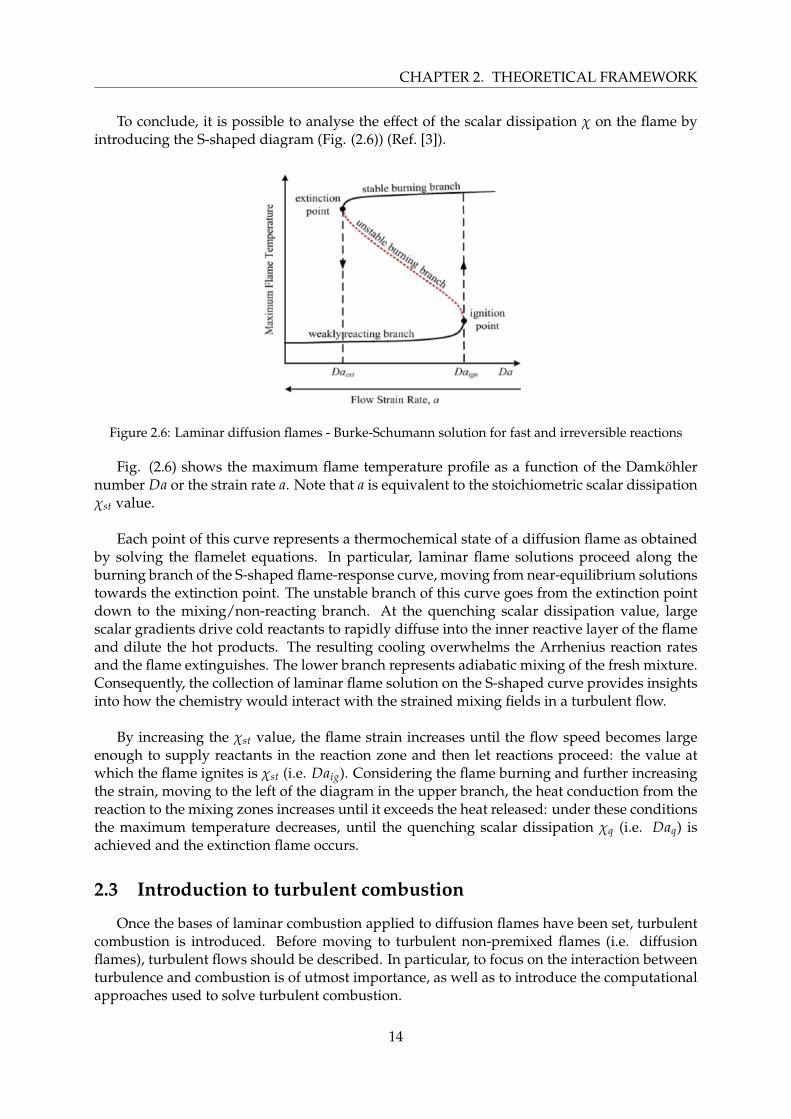
To conclude, it is possible to analyse the effect of the scalar dissipation χ on the flame byintroducing the S-shaped diagram (Fig. (2.6)) (Ref. [3]).
Figure 2.6: Laminar diffusion flames - Burke-Schumann solution for fast and irreversible reactions
Fig. (2.6) shows the maximum flame temperature profile as a function of the Damkohlernumber Da or the strain rate a. Note that a is equivalent to the stoichiometric scalar dissipationχst value.
Each point of this curve represents a thermochemical state of a diffusion flame as obtainedby solving the flamelet equations. In particular, laminar flame solutions proceed along theburning branch of the S-shaped flame-response curve, moving from near-equilibrium solutionstowards the extinction point. The unstable branch of this curve goes from the extinction pointdown to the mixing/non-reacting branch. At the quenching scalar dissipation value, largescalar gradients drive cold reactants to rapidly diffuse into the inner reactive layer of the flameand dilute the hot products. The resulting cooling overwhelms the Arrhenius reaction ratesand the flame extinguishes. The lower branch represents adiabatic mixing of the fresh mixture.Consequently, the collection of laminar flame solution on the S-shaped curve provides insightsinto how the chemistry would interact with the strained mixing fields in a turbulent flow.
By increasing the χst value, the flame strain increases until the flow speed becomes largeenough to supply reactants in the reaction zone and then let reactions proceed: the value atwhich the flame ignites is χst (i.e. Daig). Considering the flame burning and further increasingthe strain, moving to the left of the diagram in the upper branch, the heat conduction from thereaction to the mixing zones increases until it exceeds the heat released: under these conditionsthe maximum temperature decreases, until the quenching scalar dissipation χq (i.e. Daq) isachieved and the extinction flame occurs.
2.3 Introduction to turbulent combustion
Once the bases of laminar combustion applied to diffusion flames have been set, turbulentcombustion is introduced. Before moving to turbulent non-premixed flames (i.e. diffusionflames), turbulent flows should be described. In particular, to focus on the interaction betweenturbulence and combustion is of utmost importance, as well as to introduce the computationalapproaches used to solve turbulent combustion.
14
CHAPTER 2. THEORETICAL FRAMEWORK
2.3.1 Turbulent flows
By definition, turbulence is not a flow property (such as density or viscosity). Turbulenceis considered a flow state, since it is not depending on its origin and it is characterised bysudden and irregular fluctuations in the flow properties (for example, velocity or pressure). Inaddition, a turbulent flow is irrotational (vortices) and highly diffusive and dissipative.
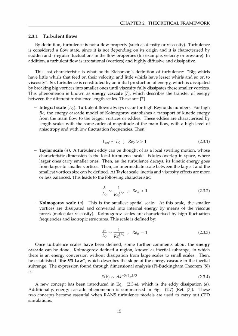
This last characteristic is what holds Richarson’s definition of turbulence: ”Big whirlshave little whirls that feed on their velocity, and little whirls have lesser whirls and so on toviscosity”. So, turbulence is constituted by an initial production of energy, which is dissipatedby breaking big vortices into smaller ones until viscosity fully dissipates these smaller vortices.This phenomenon is known as energy cascade [7], which describes the transfer of energybetween the different turbulence length scales. These are: [7]
− Integral scale (L0). Turbulent flows always occur for high Reynolds numbers. For highRe, the energy cascade model of Kolmogorov establishes a transport of kinetic energyfrom the main flow to the bigger vortices or eddies. These eddies are characterised bylength scales with the same order of magnitude of the main flow, with a high level ofanisotropy and with low fluctuation frequencies. Then:
Lre f ∼ L0 ; Re0 >> 1 (2.3.1)
− Taylor scale (λ). A turbulent eddy can be thought of as a local swirling motion, whosecharacteristic dimension is the local turbulence scale. Eddies overlap in space, wherelarger ones carry smaller ones. Then, as the turbulence decays, its kinetic energy goesfrom larger to smaller vortices. Then, an intermediate scale between the largest and thesmallest vortices size can be defined. At Taylor scale, inertia and viscosity effects are moreor less balanced. This leads to the following characteristic:
λ
L0∼ 1
Re1/20
; Reλ > 1 (2.3.2)
− Kolmogorov scale (µ). This is the smallest spatial scale. At this scale, the smallervortices are dissipated and converted into internal energy by means of the viscousforces (molecular viscosity). Kolmogorov scales are characterised by high fluctuationfrequencies and isotropic structures. This scale is defined by:
µ
L0∼ 1
Re3/40
; Reµ = 1 (2.3.3)
Once turbulence scales have been defined, some further comments about the energycascade can be done. Kolmogorov defined a region, known as inertial subrange, in whichthere is an energy conversion without dissipation from large scales to small scales. Then,he established ”the 5/3 Law”, which describes the slope of the energy cascade in the inertialsubrange. The expression found through dimensional analysis (Pi-Buckingham Theorem [8])is:
E(k) ∼ Ak−5/3ε2/3 (2.3.4)
A new concept has been introduced in Eq. (2.3.4), which is the eddy dissipation (ε).Additionally, energy cascade phenomenon is summarised in Fig. (2.7) (Ref. [7]). Thesetwo concepts become essential when RANS turbulence models are used to carry out CFDsimulations.
15
CHAPTER 2. THEORETICAL FRAMEWORK
(a) Evolution of the turbulent kinetic energy (b) Ranges and length scales
Figure 2.7: Introduction to turbulent combustion - Energy Cascade
2.3.2 Interaction between combustion and turbulence
Turbulent combustion results from the two-way interaction of chemistry and turbulence.When a flame interacts with a turbulent flow, turbulence is modified by combustion because ofthe strong flow accelerations through the flame front induced by heat release, and because ofthe large changes in kinematic viscosity associated with temperature changes. This mechanism,named flame-generated turbulence, may generate turbulence or damp it (re-laminarizationdue to combustion). On the other hand, turbulence alters the flame structure, may enhancechemical reactions increasing the reactions rates, but also, in extreme cases, completely inhibitit, leading to flame quenching.
2.3.3 Computational approaches for turbulent combustion
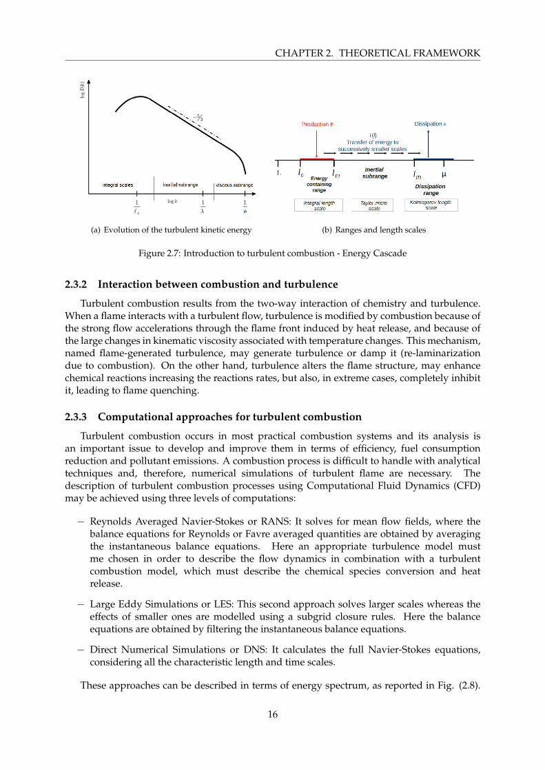
Turbulent combustion occurs in most practical combustion systems and its analysis isan important issue to develop and improve them in terms of efficiency, fuel consumptionreduction and pollutant emissions. A combustion process is difficult to handle with analyticaltechniques and, therefore, numerical simulations of turbulent flame are necessary. Thedescription of turbulent combustion processes using Computational Fluid Dynamics (CFD)may be achieved using three levels of computations:
− Reynolds Averaged Navier-Stokes or RANS: It solves for mean flow fields, where thebalance equations for Reynolds or Favre averaged quantities are obtained by averagingthe instantaneous balance equations. Here an appropriate turbulence model mustme chosen in order to describe the flow dynamics in combination with a turbulentcombustion model, which must describe the chemical species conversion and heatrelease.
− Large Eddy Simulations or LES: This second approach solves larger scales whereas theeffects of smaller ones are modelled using a subgrid closure rules. Here the balanceequations are obtained by filtering the instantaneous balance equations.
− Direct Numerical Simulations or DNS: It calculates the full Navier-Stokes equations,considering all the characteristic length and time scales.
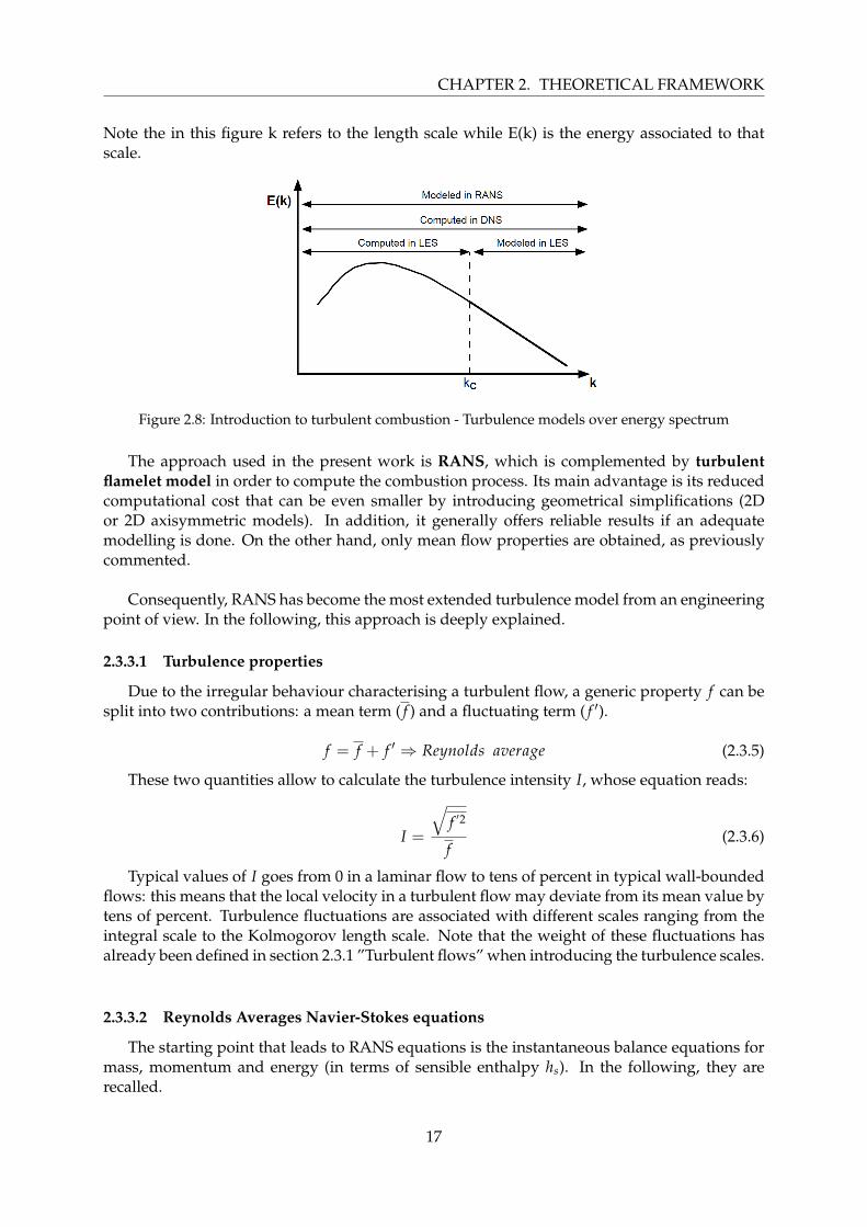
These approaches can be described in terms of energy spectrum, as reported in Fig. (2.8).
16
CHAPTER 2. THEORETICAL FRAMEWORK
Note the in this figure k refers to the length scale while E(k) is the energy associated to thatscale.
Figure 2.8: Introduction to turbulent combustion - Turbulence models over energy spectrum
The approach used in the present work is RANS, which is complemented by turbulentflamelet model in order to compute the combustion process. Its main advantage is its reducedcomputational cost that can be even smaller by introducing geometrical simplifications (2Dor 2D axisymmetric models). In addition, it generally offers reliable results if an adequatemodelling is done. On the other hand, only mean flow properties are obtained, as previouslycommented.
Consequently, RANS has become the most extended turbulence model from an engineeringpoint of view. In the following, this approach is deeply explained.
2.3.3.1 Turbulence properties
Due to the irregular behaviour characterising a turbulent flow, a generic property f can besplit into two contributions: a mean term ( f ) and a fluctuating term ( f ′).
f = f + f ′ ⇒ Reynolds average (2.3.5)
These two quantities allow to calculate the turbulence intensity I, whose equation reads:
I =
√f ′2
f(2.3.6)
Typical values of I goes from 0 in a laminar flow to tens of percent in typical wall-boundedflows: this means that the local velocity in a turbulent flow may deviate from its mean value bytens of percent. Turbulence fluctuations are associated with different scales ranging from theintegral scale to the Kolmogorov length scale. Note that the weight of these fluctuations hasalready been defined in section 2.3.1 ”Turbulent flows” when introducing the turbulence scales.
2.3.3.2 Reynolds Averages Navier-Stokes equations
The starting point that leads to RANS equations is the instantaneous balance equations formass, momentum and energy (in terms of sensible enthalpy hs). In the following, they arerecalled.
17
CHAPTER 2. THEORETICAL FRAMEWORK
− Mass conservation:
∂ρ
∂t+
∂ρui
∂xi= 0 (2.3.7)
− Momentum conservation:
∂
∂t(ρui) +
∂
∂xj(ρuiuj) +
∂p∂xi
=∂τij
∂xj(2.3.8)
− Mass fraction conservation for the k-th species:
∂ρYk
∂t+
∂
∂xi(ρuiYk) = −
∂
∂xi(Vk,iYk) + ωk f or k = 1, ..., N (2.3.9)
− Energy equation in terms of sensible enthalpy hs:
∂ρhs
∂t+
∂
∂xi(ρuihs) =
DpDt
+∂
∂xi
(λ
∂T∂xi
)− ∂
∂xi
(ρ
N
∑k=1
Vk,iYkhs,k
)+ τij
∂ui
∂xj+ ωT (2.3.10)
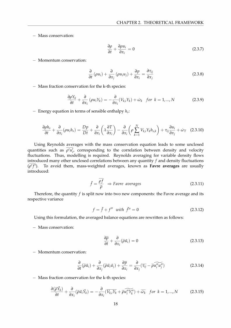
Using Reynolds averages with the mass conservation equation leads to some unclosedquantities such as ρ′u′i, corresponding to the correlation between density and velocityfluctuations. Thus, modelling is required. Reynolds averaging for variable density flowsintroduced many other unclosed correlations between any quantity f and density fluctuations(ρ′ f ′). To avoid them, mass-weighted averages, known as Favre averages are usuallyintroduced:
f =ρ fρ⇒ Favre averages (2.3.11)
Therefore, the quantity f is split now into two new components: the Favre average and itsrespective variance
f = f + f ′′ with f ′′ = 0 (2.3.12)
Using this formulation, the averaged balance equations are rewritten as follows:
− Mass conservation:
∂ρ
∂t+
∂
∂xi(ρui) = 0 (2.3.13)
− Momentum conservation:
∂
∂t(ρui) +
∂
∂xj(ρuiuj) +
∂p∂xi
=∂
∂xj(τij − ρu′′i u′′j ) (2.3.14)
− Mass fraction conservation for the k-th species:
∂(ρYk)
∂t+
∂
∂xi(ρuiYk) = −
∂
∂xi(Vk,iYk + ρu′′i Y′′k ) + ωk f or k = 1, ..., N (2.3.15)
18
CHAPTER 2. THEORETICAL FRAMEWORK
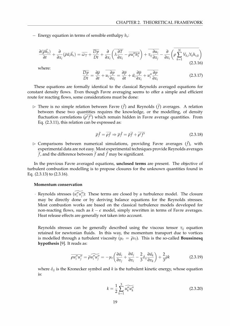
− Energy equation in terms of sensible enthalpy hs:
∂(ρhs)
∂t+
∂
∂xi(ρui hs) = ωT +
DpDt
+∂
∂xi
(λ
∂T∂xi− ρu′′i h′′s
)+ τij
∂ui
∂xj− ∂
∂xi
(ρ
N
∑k=1
Vk,iYkhs,k
)(2.3.16)
where:DpDt
=∂ρ
∂t+ ui
∂p∂xi
=∂p∂t
+ ui∂p∂xi
+ u′′i∂p∂xi
(2.3.17)
These equations are formally identical to the classical Reynolds averaged equations forconstant density flows. Even though Favre averaging seems to offer a simple and efficientroute for reacting flows, some considerations must be done:
B There is no simple relation between Favre ( f ) and Reynolds ( f ) averages. A relationbetween these two quantities requires the knowledge, or the modelling, of densityfluctuation correlations (ρ′ f ′) which remain hidden in Favre average quantities. FromEq. (2.3.11), this relation can be expressed as:
ρ f = ρ f ⇒ ρ f = ρ f + ρ′ f ′ (2.3.18)
B Comparisons between numerical simulations, providing Favre averages ( f ), withexperimental data are not easy. Most experimental techniques provide Reynolds averagesf , and the difference between f and f may be significant.
In the previous Favre averaged equations, unclosed terms are present. The objective ofturbulent combustion modelling is to propose closures for the unknown quantities found inEq. (2.3.13) to (2.3.16).
Momentum conservation
· Reynolds stresses (u′′i u′′j ): These terms are closed by a turbulence model. The closuremay be directly done or by deriving balance equations for the Reynolds stresses.Most combustion works are based on the classical turbulence models developed fornon-reacting flows, such as k − ε model, simply rewritten in terms of Favre averages.Heat release effects are generally not taken into account.
Reynolds stresses can be generally described using the viscous tensor τij equationretained for newtonian fluids. In this way, the momentum transport due to vorticesis modelled through a turbulent viscosity (µt = ρνt). This is the so-called Boussinesqhypothesis [9]. It reads as:
ρu′′i u′′j = ρu′′i u′′j = −µt
(∂ui
∂xj+
∂uj
∂xi− 2
3δij
∂uk
∂xk
)+
23
ρk (2.3.19)
where δij is the Kronecker symbol and k is the turbulent kinetic energy, whose equationis:
k =12
3
∑k=1
u′′k u′′k (2.3.20)
19
CHAPTER 2. THEORETICAL FRAMEWORK
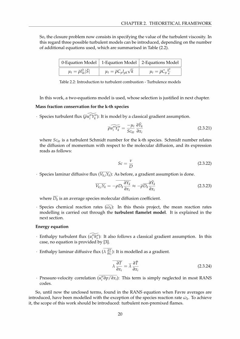
So, the closure problem now consists in specifying the value of the turbulent viscosity. Inthis regard three possible turbulent models can be introduced, depending on the numberof additional equations used, which are summarised in Table (2.2).
0-Equation Model 1-Equation Model 2-Equations Model
µt = ρl2m|S| µt = ρCµlρk
√k µt = ρCµ
k2
ε
Table 2.2: Introduction to turbulent combustion - Turbulence models
In this work, a two-equations model is used, whose selection is justified in next chapter.
Mass fraction conservation for the k-th species
· Species turbulent flux (ρu′′i Y′′k ): It is model by a classical gradient assumption.
ρu′′i Y′′k =−µt
Sckt
∂Yk
∂xi(2.3.21)
where Sckt is a turbulent Schmidt number for the k-th species. Schmidt number relatesthe diffusion of momentum with respect to the molecular diffusion, and its expressionreads as follows:
Sc =ν
D(2.3.22)
· Species laminar diffusive flux (Vk,iYk): As before, a gradient assumption is done.
Vk,iYk = −ρDk∂Yk
∂xi≈ −ρDk
∂Yk
∂xi(2.3.23)
where Dk is an average species molecular diffusion coefficient.
· Species chemical reaction rates (ωk): In this thesis project, the mean reaction ratesmodelling is carried out through the turbulent flamelet model. It is explained in thenext section.
Energy equation
· Enthalpy turbulent flux (u′′i h′′s ): It also follows a classical gradient assumption. In thiscase, no equation is provided by [3].
· Enthalpy laminar diffusive flux (λ ∂T∂xi
): It is modelled as a gradient.
λ∂T∂xi
= λ∂T∂xi
(2.3.24)
· Pressure-velocity correlation (u′′i ∂p/∂xi): This term is simply neglected in most RANScodes.
So, until now the unclosed terms, found in the RANS equation when Favre averages areintroduced, have been modelled with the exception of the species reaction rate ωk. To achieveit, the scope of this work should be introduced: turbulent non-premixed flames.
20
CHAPTER 2. THEORETICAL FRAMEWORK
2.4 Turbulent non-premixed flames
Turbulent non-premixed flames are encountered in a large number of industrial systemsfor two main reasons. First, compared to premixed flames, non-premixed burners are simplerto design and to build because a perfect reactant mixing, in given proportions, is not required.Non-premixed flames are also safer to operate as they don not exhibit propagation speeds andcannot flashback or autoignite in undesired locations. Accordingly, turbulent non-premixedflame modelling is one of the most usual challenges assigned to combustion codes in industrialapplications.
As explained for laminar diffusion flames, reactant species have to reach, by moleculardiffusion, the flame front before reaction. Hence, non-premixed flames are also called diffusionflames. During this travel, they are exposed to turbulence and their diffusion speeds maybe strongly modified by turbulent motions. The overall reaction rate is often limited by thespecies molecular diffusion towards the flame front. Then, in many models, the chemicalreaction is assumed to be fast, or infinitely fast, compared to transport processes.
2.4.1 Main characteristics
Additionally to the characteristics commented for laminar diffusion flames, which are stillvalid, several points should be remarked (mainly due to the inclusion of turbulence effects):
− Diffusion flames are more sensitive to stretch than turbulent premixed flames: criticalstretch values for extinction of diffusion flames are one order of magnitude smaller thanfor premixed flames. A diffusion flame is more likely to be quenched by turbulentfluctuations.
− Buoyancy effects may be enhanced: pressure gradients or gravity forces inducedifferential effects on fuel, oxidizer and combustion products streams. For example, purehydrogen/air flames use reactants having quite different densities. Molecular diffusionmay also be strongly affected (differential diffusivity effects).
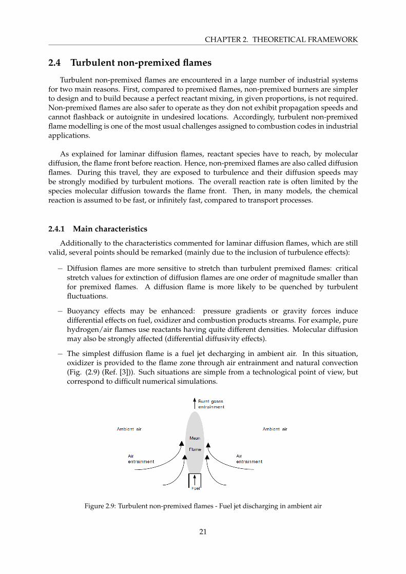
− The simplest diffusion flame is a fuel jet decharging in ambient air. In this situation,oxidizer is provided to the flame zone through air entrainment and natural convection(Fig. (2.9) (Ref. [3])). Such situations are simple from a technological point of view, butcorrespond to difficult numerical simulations.
Figure 2.9: Turbulent non-premixed flames - Fuel jet discharging in ambient air
21
CHAPTER 2. THEORETICAL FRAMEWORK
− Non-premixed flame stabilization is also a challenging problem, which requires a deeperdiscussion.
2.4.1.1 Flame stabilization
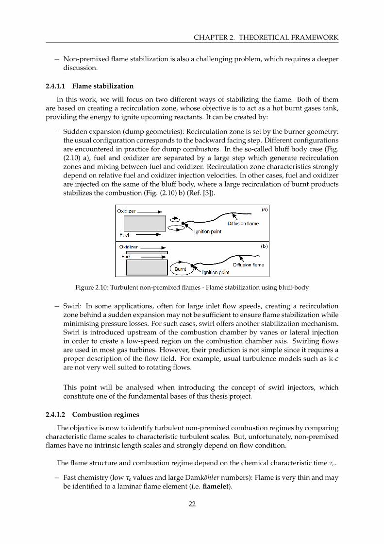
In this work, we will focus on two different ways of stabilizing the flame. Both of themare based on creating a recirculation zone, whose objective is to act as a hot burnt gases tank,providing the energy to ignite upcoming reactants. It can be created by:
− Sudden expansion (dump geometries): Recirculation zone is set by the burner geometry:the usual configuration corresponds to the backward facing step. Different configurationsare encountered in practice for dump combustors. In the so-called bluff body case (Fig.(2.10) a), fuel and oxidizer are separated by a large step which generate recirculationzones and mixing between fuel and oxidizer. Recirculation zone characteristics stronglydepend on relative fuel and oxidizer injection velocities. In other cases, fuel and oxidizerare injected on the same of the bluff body, where a large recirculation of burnt productsstabilizes the combustion (Fig. (2.10) b) (Ref. [3]).
Figure 2.10: Turbulent non-premixed flames - Flame stabilization using bluff-body
− Swirl: In some applications, often for large inlet flow speeds, creating a recirculationzone behind a sudden expansion may not be sufficient to ensure flame stabilization whileminimising pressure losses. For such cases, swirl offers another stabilization mechanism.Swirl is introduced upstream of the combustion chamber by vanes or lateral injectionin order to create a low-speed region on the combustion chamber axis. Swirling flowsare used in most gas turbines. However, their prediction is not simple since it requires aproper description of the flow field. For example, usual turbulence models such as k-εare not very well suited to rotating flows.
This point will be analysed when introducing the concept of swirl injectors, whichconstitute one of the fundamental bases of this thesis project.
2.4.1.2 Combustion regimes
The objective is now to identify turbulent non-premixed combustion regimes by comparingcharacteristic flame scales to characteristic turbulent scales. But, unfortunately, non-premixedflames have no intrinsic length scales and strongly depend on flow condition.
The flame structure and combustion regime depend on the chemical characteristic time τc.
− Fast chemistry (low τc values and large Damkohler numbers): Flame is very thin and maybe identified to a laminar flame element (i.e. flamelet).
22
CHAPTER 2. THEORETICAL FRAMEWORK
− Larger values of τc: Departures from laminar flame structures to unsteady effects areexpected.
− Low Damkohler numbers: Extinction occurs.
Note that Damkohler number (also known as time ratio) is defined as:
Da =τt
τc(2.4.1)
where τt is the shortest turbulent time, corresponding to the worst case, whereas τc representsthe chemical time. This expression can be modelled in the following way:
Da ≈ 2√
RetDa f l (2.4.2)
with Da f l = 1/(τcχst).
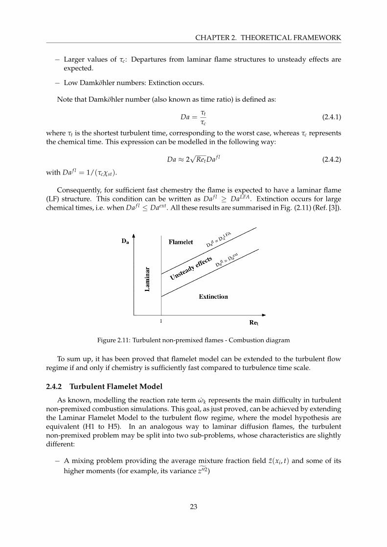
Consequently, for sufficient fast chemestry the flame is expected to have a laminar flame(LF) structure. This condition can be written as Da f l ≥ DaLFA. Extinction occurs for largechemical times, i.e. when Da f l ≤ Daext. All these results are summarised in Fig. (2.11) (Ref. [3]).
Figure 2.11: Turbulent non-premixed flames - Combustion diagram
To sum up, it has been proved that flamelet model can be extended to the turbulent flowregime if and only if chemistry is sufficiently fast compared to turbulence time scale.
2.4.2 Turbulent Flamelet Model
As known, modelling the reaction rate term ωk represents the main difficulty in turbulentnon-premixed combustion simulations. This goal, as just proved, can be achieved by extendingthe Laminar Flamelet Model to the turbulent flow regime, where the model hypothesis areequivalent (H1 to H5). In an analogous way to laminar diffusion flames, the turbulentnon-premixed problem may be split into two sub-problems, whose characteristics are slightlydifferent:
− A mixing problem providing the average mixture fraction field z(xi, t) and some of itshigher moments (for example, its variance z′′2)
23
CHAPTER 2. THEORETICAL FRAMEWORK
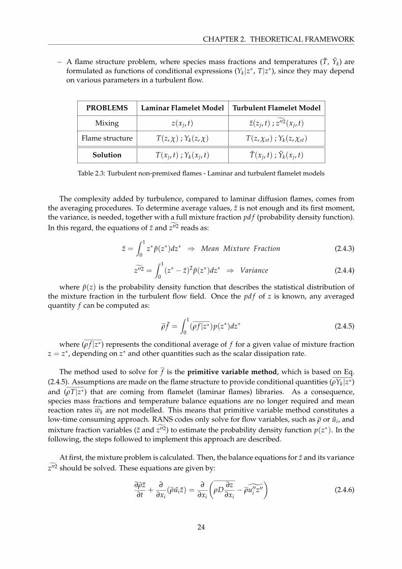
− A flame structure problem, where species mass fractions and temperatures (T, Yk) areformulated as functions of conditional expressions (Yk|z∗, T|z∗), since they may dependon various parameters in a turbulent flow.
PROBLEMS Laminar Flamelet Model Turbulent Flamelet Model
Mixing z(xj, t) z(zj, t) ; z′′2(xj, t)
Flame structure T(z, χ) ; Yk(z, χ) T(z, χst) ; Yk(z, χst)
Solution T(xj, t) ; Yk(xj, t) T(xj, t) ; Yk(xj, t)
Table 2.3: Turbulent non-premixed flames - Laminar and turbulent flamelet models
The complexity added by turbulence, compared to laminar diffusion flames, comes fromthe averaging procedures. To determine average values, z is not enough and its first moment,the variance, is needed, together with a full mixture fraction pd f (probability density function).In this regard, the equations of z and z′′2 reads as:
z =∫ 1
0z∗ p(z∗)dz∗ ⇒ Mean Mixture Fraction (2.4.3)
z′′2 =∫ 1
0(z∗ − z)2 p(z∗)dz∗ ⇒ Variance (2.4.4)
where p(z) is the probability density function that describes the statistical distribution ofthe mixture fraction in the turbulent flow field. Once the pd f of z is known, any averagedquantity f can be computed as:
ρ f =∫ 1
0(ρ f |z∗)p(z∗)dz∗ (2.4.5)
where (ρ f |z∗) represents the conditional average of f for a given value of mixture fractionz = z∗, depending on z∗ and other quantities such as the scalar dissipation rate.
The method used to solve for f is the primitive variable method, which is based on Eq.(2.4.5). Assumptions are made on the flame structure to provide conditional quantities (ρYk|z∗)and (ρT|z∗) that are coming from flamelet (laminar flames) libraries. As a consequence,species mass fractions and temperature balance equations are no longer required and meanreaction rates wk are not modelled. This means that primitive variable method constitutes alow-time consuming approach. RANS codes only solve for flow variables, such as ρ or ui, andmixture fraction variables (z and z′′2) to estimate the probability density function p(z∗). In thefollowing, the steps followed to implement this approach are described.
At first, the mixture problem is calculated. Then, the balance equations for z and its variancez′′2 should be solved. These equations are given by:
∂ρz∂t
+∂
∂xi(ρui z) =
∂
∂xi
(ρD
∂z∂xi− ρu′′i z′′
)(2.4.6)
24
CHAPTER 2. THEORETICAL FRAMEWORK
∂ρz′′2
∂t+
∂
∂xi(ρui z′′2) =
∂
∂xi
(ρ
νt
Sct1
∂z′′2
∂xi
)+ 2ρ
νt
Sct2
∂z∂xi
z∂xi− cρ
ε
kz′′2 (2.4.7)
with c as a model constant of order unity.
Some simplifications can be introduced for these equations. Eq. (2.4.7) can be directlyrewritten as:
∂ρz′′2
∂t+
∂
∂xi(ρui z′′2) =
∂
∂xi
(µt
Sct
∂z′′2
∂xi
)+ Cgρνt
(∂z∂xi
)2
− Cdρε
kz′′2 (2.4.8)
where Cg and Cd are model constants equal to 2.86 and 2, respectively, according to [3].
Regarding Eq. (2.4.6), the production term ρu′′i z′′ can be expressed as:
ρu′′i z′′ = − µt
Sct
∂z∂xi
(2.4.9)
Recalling H1 and H2 assumptions (i.e. Le = 1), the following property is verified:
Sc = Pr · Le⇒ Sc = Pr withµ
ρD= Sc⇒ ρD =
µ
Sc(2.4.10)
Note that Prandtl number (Pr) is defining the ratio between momentum diffusion andmolecular diffusion.
Pr =νρCp
λ(2.4.11)
Consequently, the RHS of Eq. (2.4.6) can be rewritten as:
∂
∂xi
(µ
Sc+
µt
Sct
)∂z∂xi
(2.4.12)
In the previous equation, the term in parenthesis represents the effective transportcoefficient, which is defined as:
Γe f f =µ
Sc+
µt
Sct(2.4.13)
Then:
∂ρz∂t
+∂
∂xi(ρui z) =
∂
∂xi
(Γe f f
∂z∂xi
)(2.4.14)
Usually turbulent transport is of order of magnitude higher than its laminar counterpart.Therefore, in many codes the laminar Schmidt number Sc is neglected:
Γe f f =µe f f
Sct; with µe f f = µlam + µt (2.4.15)
So, after introducing all these simplifications, balance equations for z and z′′2 are given byEqs. (2.4.8) and (2.4.14).
Once the balance equations required to solve the mixture problem are defined, it isnecessary to introduce their corresponding pd f functions. They can be both presumed and
25
CHAPTER 2. THEORETICAL FRAMEWORK
obtained solving for a balance equation. The most widely used presumed pd f for the mixturefraction z is the β− f unction, whose dependence is limited to the mean mixture fraction andits variance. Its equation is expressed as:
p(z) =1
B(a, b)· za−1 · (1− z)b−1 =
Γ(a + b)Γ(a)Γ(b)
· za−1 · (1− z)b−1 (2.4.16)
where B(a, b) is a normalization factor, Γ is a function and a and b are two parametersdepending on z and z′′2, whose equations are reported below. [3]
B(a, b) =∫ 1
0za−1 · (1− z)b−1dz (2.4.17)
a = z ·(
z(1− z)
z′′2− 1)
; b = a ·(
1− zz
)(2.4.18)
Γ(x) =∫ +∞
0e−t · tx−1dt (2.4.19)
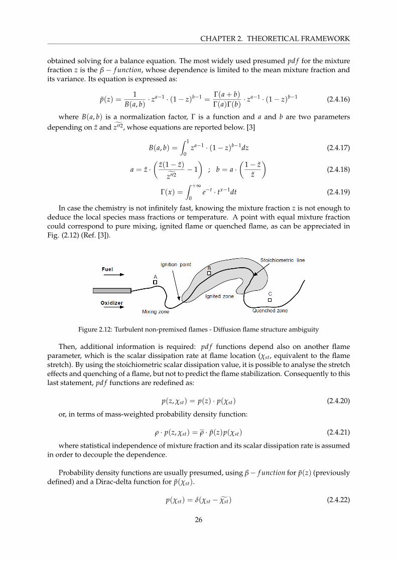
In case the chemistry is not infinitely fast, knowing the mixture fraction z is not enough todeduce the local species mass fractions or temperature. A point with equal mixture fractioncould correspond to pure mixing, ignited flame or quenched flame, as can be appreciated inFig. (2.12) (Ref. [3]).
Figure 2.12: Turbulent non-premixed flames - Diffusion flame structure ambiguity
Then, additional information is required: pd f functions depend also on another flameparameter, which is the scalar dissipation rate at flame location (χst, equivalent to the flamestretch). By using the stoichiometric scalar dissipation value, it is possible to analyse the stretcheffects and quenching of a flame, but not to predict the flame stabilization. Consequently to thislast statement, pd f functions are redefined as:
p(z, χst) = p(z) · p(χst) (2.4.20)
or, in terms of mass-weighted probability density function:
ρ · p(z, χst) = ρ · p(z)p(χst) (2.4.21)
where statistical independence of mixture fraction and its scalar dissipation rate is assumedin order to decouple the dependence.
Probability density functions are usually presumed, using β− f unction for p(z) (previouslydefined) and a Dirac-delta function for p(χst).
p(χst) = δ(χst − χst) (2.4.22)
26
CHAPTER 2. THEORETICAL FRAMEWORK
A more physical approach is to use log normal distributions for p(χst). It is:
p(χst) =1
χstσ√
2π· exp
(− (ln(χst)− µ)2
2σ2
)(2.4.23)
where µ and σ are linked to mean value of χst and its variance χ′′2st .
χst =∫ +∞
0χst p(χst)dχst = exp
(µ +
σ2
2
)(2.4.24)
χ′′2st = χ2st · exp(σ2 − 1) (2.4.25)
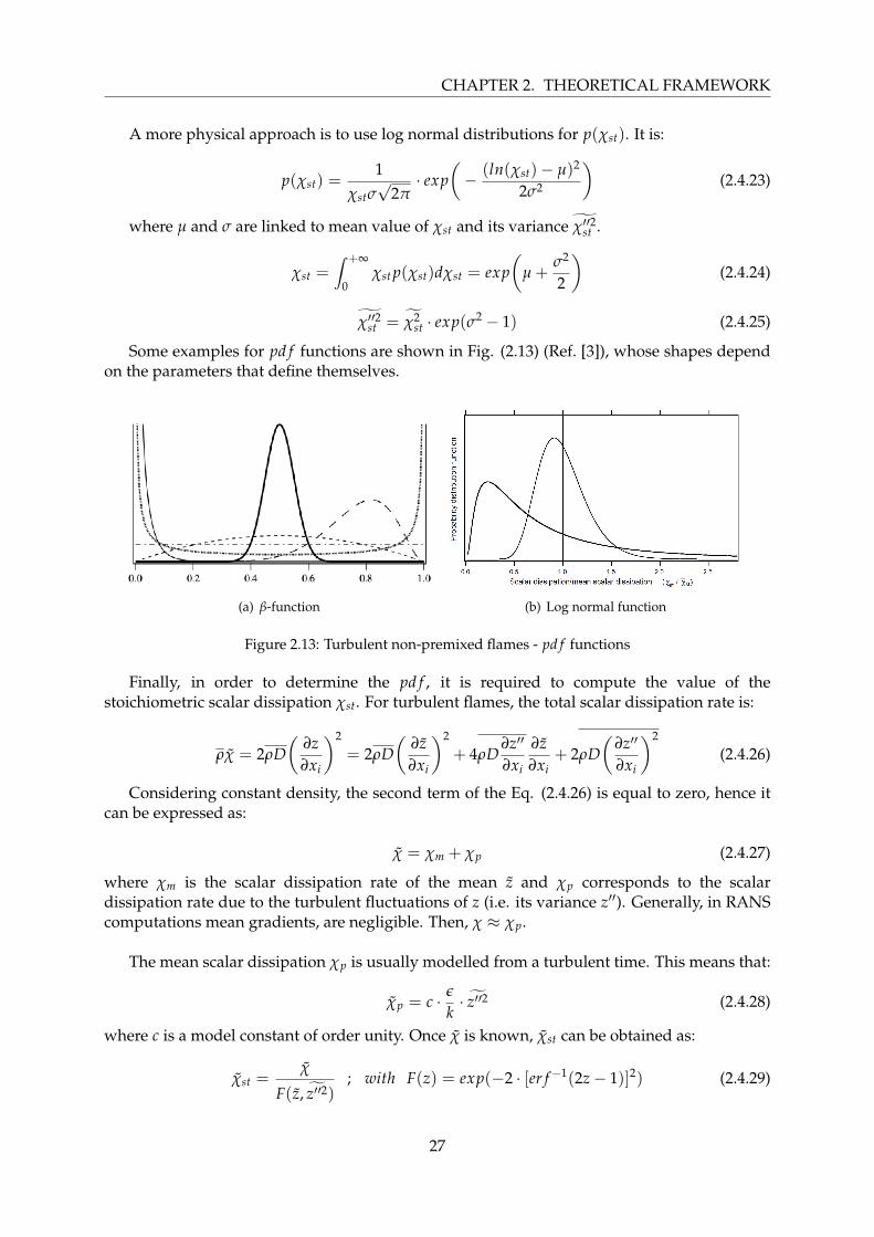
Some examples for pd f functions are shown in Fig. (2.13) (Ref. [3]), whose shapes dependon the parameters that define themselves.
(a) β-function (b) Log normal function
Figure 2.13: Turbulent non-premixed flames - pd f functions
Finally, in order to determine the pd f , it is required to compute the value of thestoichiometric scalar dissipation χst. For turbulent flames, the total scalar dissipation rate is:
ρχ = 2ρD(
∂z∂xi
)2
= 2ρD(
∂z∂xi
)2
+ 4ρD∂z′′
∂xi
∂z∂xi
+ 2ρD(
∂z′′
∂xi
)2
(2.4.26)
Considering constant density, the second term of the Eq. (2.4.26) is equal to zero, hence itcan be expressed as:
χ = χm + χp (2.4.27)
where χm is the scalar dissipation rate of the mean z and χp corresponds to the scalardissipation rate due to the turbulent fluctuations of z (i.e. its variance z′′). Generally, in RANScomputations mean gradients, are negligible. Then, χ ≈ χp.
The mean scalar dissipation χp is usually modelled from a turbulent time. This means that:
χp = c · ε
k· z′′2 (2.4.28)
where c is a model constant of order unity. Once χ is known, χst can be obtained as:
χst =χ
F(z, z′′2); with F(z) = exp(−2 · [er f−1(2z− 1)]2) (2.4.29)
27
CHAPTER 2. THEORETICAL FRAMEWORK
In practice, the approximation χ = χst is used.
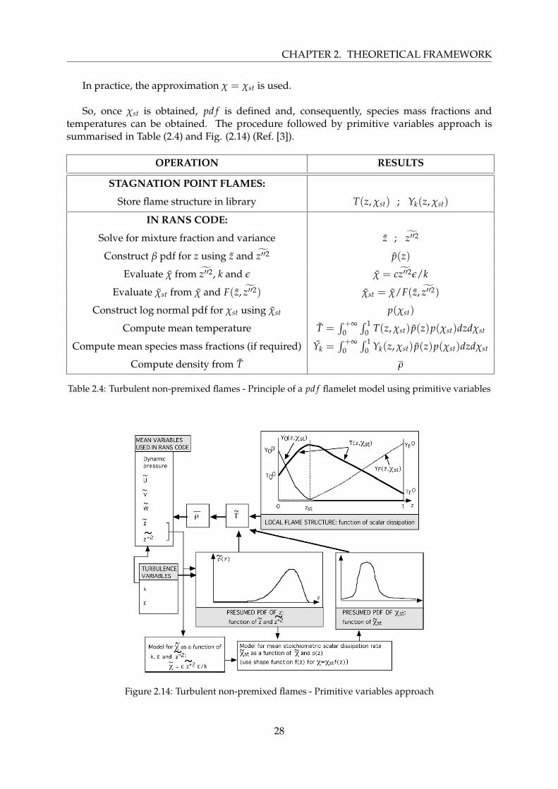
So, once χst is obtained, pd f is defined and, consequently, species mass fractions andtemperatures can be obtained. The procedure followed by primitive variables approach issummarised in Table (2.4) and Fig. (2.14) (Ref. [3]).
OPERATION RESULTS
STAGNATION POINT FLAMES:
Store flame structure in library T(z, χst) ; Yk(z, χst)
IN RANS CODE:
Solve for mixture fraction and variance z ; z′′2
Construct β pdf for z using z and z′′2 p(z)
Evaluate χ from z′′2, k and ε χ = cz′′2ε/k
Evaluate χst from χ and F(z, z′′2) χst = χ/F(z, z′′2)
Construct log normal pdf for χst using χst p(χst)
Compute mean temperature T =∫ +∞
0
∫ 10 T(z, χst) p(z)p(χst)dzdχst
Compute mean species mass fractions (if required) Yk =∫ +∞
0
∫ 10 Yk(z, χst) p(z)p(χst)dzdχst
Compute density from T ρ
Table 2.4: Turbulent non-premixed flames - Principle of a pd f flamelet model using primitive variables
Figure 2.14: Turbulent non-premixed flames - Primitive variables approach
28
CHAPTER 2. THEORETICAL FRAMEWORK
2.5 Swirling flames
Once non-premixed flames and the computational approach used to simulate turbulentcombustion problems have been defined, swirling flames are introduced. At this section, thedescription of a swirling flow and its application in the combustion field is reported.
2.5.1 Introduction to swirling flows
Swirling flows can be defined as a combination of vortex flow and axial velocity, whichmakes the fluid move in helicoidal trajectories. This is the reason why swirled flows areusually described in cylindrical coordinates (x, r, ϕ), allowing a better understanding of theflow motion.
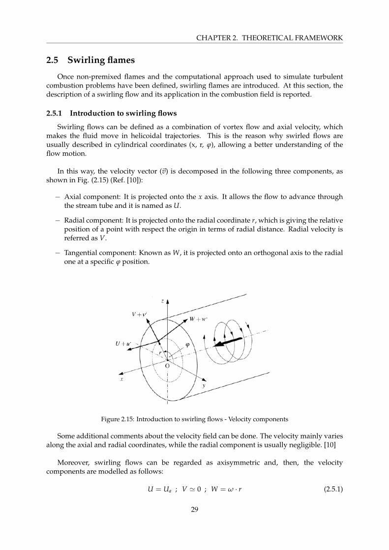
In this way, the velocity vector (~v) is decomposed in the following three components, asshown in Fig. (2.15) (Ref. [10]):
− Axial component: It is projected onto the x axis. It allows the flow to advance throughthe stream tube and it is named as U.
− Radial component: It is projected onto the radial coordinate r, which is giving the relativeposition of a point with respect the origin in terms of radial distance. Radial velocity isreferred as V.
− Tangential component: Known as W, it is projected onto an orthogonal axis to the radialone at a specific ϕ position.
Figure 2.15: Introduction to swirling flows - Velocity components
Some additional comments about the velocity field can be done. The velocity mainly variesalong the axial and radial coordinates, while the radial component is usually negligible. [10]
Moreover, swirling flows can be regarded as axisymmetric and, then, the velocitycomponents are modelled as follows:
U = Ua ; V ' 0 ; W = ω · r (2.5.1)
29
CHAPTER 2. THEORETICAL FRAMEWORK
In fact, this will be the modelling adopted when implementing the swirl boundarycondition into numerical simulations. This means that a value of axial (Ua) and angularvelocity (ω) need to be specified to generate a swirl.
One further comment about axisymmetry assumption should be done. Axisymmetryhypothesis allows to reduce the required computational domain by neglecting all thecircumferential gradients (∂/∂ϕ = 0).
In addition, this swirling flow is characterised by a highly anisotropic turbulence structureas a consequence of additional flow phenomena that are not present in simple shear flow, suchas shear component associated to ∂W/∂r; additionally to common mean shear proportional to∂U/∂r and streamline curvature. This leads to a perpetual challenge in terms of turbulencemodelling.
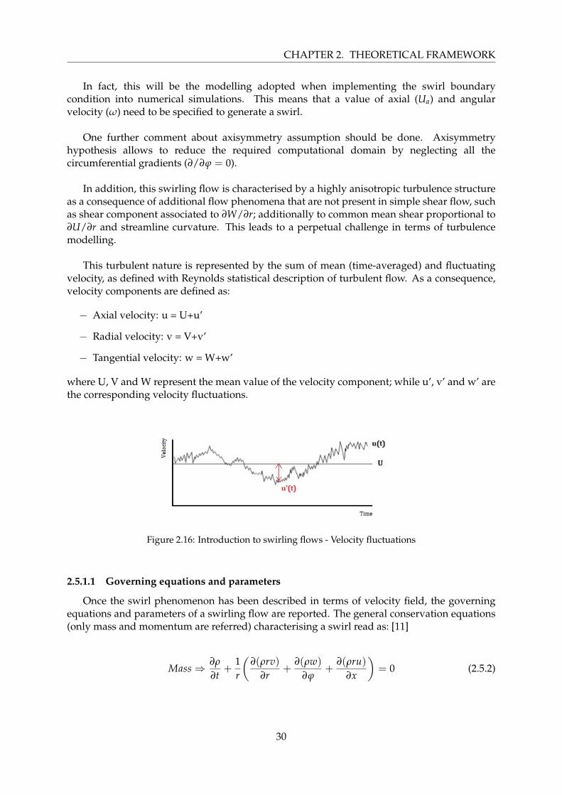
This turbulent nature is represented by the sum of mean (time-averaged) and fluctuatingvelocity, as defined with Reynolds statistical description of turbulent flow. As a consequence,velocity components are defined as:
− Axial velocity: u = U+u’
− Radial velocity: v = V+v’
− Tangential velocity: w = W+w’
where U, V and W represent the mean value of the velocity component; while u’, v’ and w’ arethe corresponding velocity fluctuations.
Figure 2.16: Introduction to swirling flows - Velocity fluctuations
2.5.1.1 Governing equations and parameters
Once the swirl phenomenon has been described in terms of velocity field, the governingequations and parameters of a swirling flow are reported. The general conservation equations(only mass and momentum are referred) characterising a swirl read as: [11]
Mass⇒ ∂ρ
∂t+
1r
(∂(ρrv)
∂r+
∂(ρw)
∂ϕ+
∂(ρru)∂x
)= 0 (2.5.2)
30
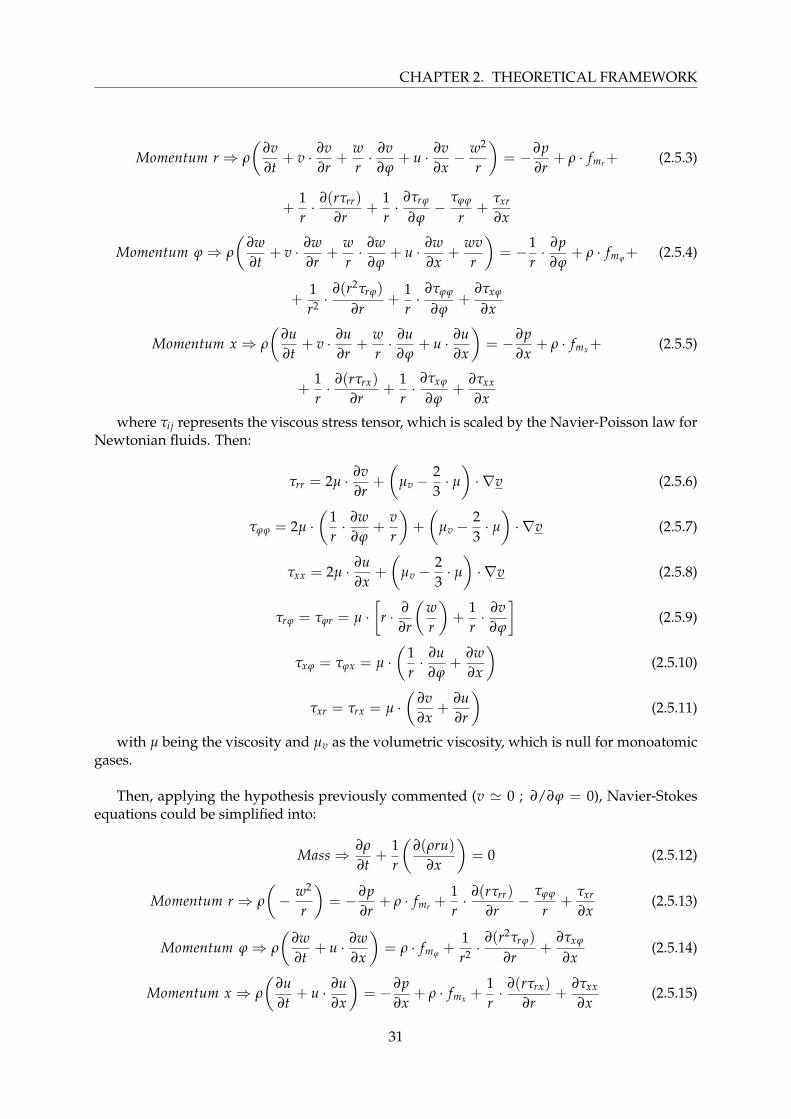
CHAPTER 2. THEORETICAL FRAMEWORK
Momentum r ⇒ ρ
(∂v∂t
+ v · ∂v∂r
+wr· ∂v
∂ϕ+ u · ∂v
∂x− w2
r
)= −∂p
∂r+ ρ · fmr+ (2.5.3)
+1r· ∂(rτrr)
∂r+
1r·
∂τrϕ
∂ϕ−
τϕϕ
r+
τxr
∂x
Momentum ϕ⇒ ρ
(∂w∂t
+ v · ∂w∂r
+wr· ∂w
∂ϕ+ u · ∂w
∂x+
wvr
)= −1
r· ∂p
∂ϕ+ ρ · fmϕ+ (2.5.4)
+1r2 ·
∂(r2τrϕ)
∂r+
1r·
∂τϕϕ
∂ϕ+
∂τxϕ
∂x
Momentum x ⇒ ρ
(∂u∂t
+ v · ∂u∂r
+wr· ∂u
∂ϕ+ u · ∂u
∂x
)= −∂p
∂x+ ρ · fmx+ (2.5.5)
+1r· ∂(rτrx)
∂r+
1r·
∂τxϕ
∂ϕ+
∂τxx
∂x
where τij represents the viscous stress tensor, which is scaled by the Navier-Poisson law forNewtonian fluids. Then:
τrr = 2µ · ∂v∂r
+
(µv −
23· µ)· ∇v (2.5.6)
τϕϕ = 2µ ·(
1r· ∂w
∂ϕ+
vr
)+
(µv −
23· µ)· ∇v (2.5.7)
τxx = 2µ · ∂u∂x
+
(µv −
23· µ)· ∇v (2.5.8)
τrϕ = τϕr = µ ·[
r · ∂
∂r
(wr
)+
1r· ∂v
∂ϕ
](2.5.9)
τxϕ = τϕx = µ ·(
1r· ∂u
∂ϕ+
∂w∂x
)(2.5.10)
τxr = τrx = µ ·(
∂v∂x
+∂u∂r
)(2.5.11)
with µ being the viscosity and µv as the volumetric viscosity, which is null for monoatomicgases.
Then, applying the hypothesis previously commented (v ' 0 ; ∂/∂ϕ = 0), Navier-Stokesequations could be simplified into:
Mass⇒ ∂ρ
∂t+
1r
(∂(ρru)
∂x
)= 0 (2.5.12)
Momentum r ⇒ ρ
(− w2
r
)= −∂p
∂r+ ρ · fmr +
1r· ∂(rτrr)
∂r−
τϕϕ
r+
τxr
∂x(2.5.13)
Momentum ϕ⇒ ρ
(∂w∂t
+ u · ∂w∂x
)= ρ · fmϕ +
1r2 ·
∂(r2τrϕ)
∂r+
∂τxϕ
∂x(2.5.14)
Momentum x ⇒ ρ
(∂u∂t
+ u · ∂u∂x
)= −∂p
∂x+ ρ · fmx +
1r· ∂(rτrx)
∂r+
∂τxx
∂x(2.5.15)
31
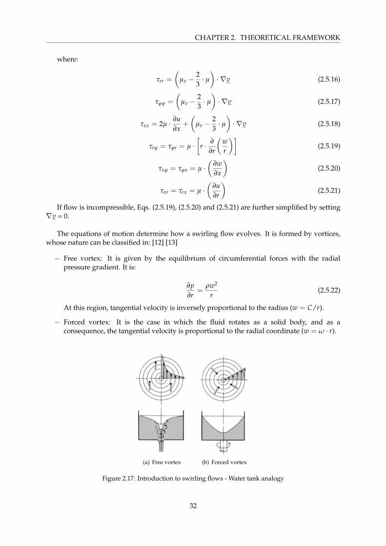
CHAPTER 2. THEORETICAL FRAMEWORK
where:
τrr =
(µv −
23· µ)· ∇v (2.5.16)
τϕϕ =
(µv −
23· µ)· ∇v (2.5.17)
τxx = 2µ · ∂u∂x
+
(µv −
23· µ)· ∇v (2.5.18)
τrϕ = τϕr = µ ·[
r · ∂
∂r
(wr
)](2.5.19)
τxϕ = τϕx = µ ·(
∂w∂x
)(2.5.20)
τxr = τrx = µ ·(
∂u∂r
)(2.5.21)
If flow is incompressible, Eqs. (2.5.19), (2.5.20) and (2.5.21) are further simplified by setting∇v = 0.
The equations of motion determine how a swirling flow evolves. It is formed by vortices,whose nature can be classified in: [12] [13]
− Free vortex: It is given by the equilibrium of circumferential forces with the radialpressure gradient. It is:
∂p∂r
=ρw2
r(2.5.22)
At this region, tangential velocity is inversely proportional to the radius (w = C/r).
− Forced vortex: It is the case in which the fluid rotates as a solid body, and as aconsequence, the tangential velocity is proportional to the radial coordinate (w = ω · r).
(a) Free vortex (b) Forced vortex
Figure 2.17: Introduction to swirling flows - Water tank analogy
32
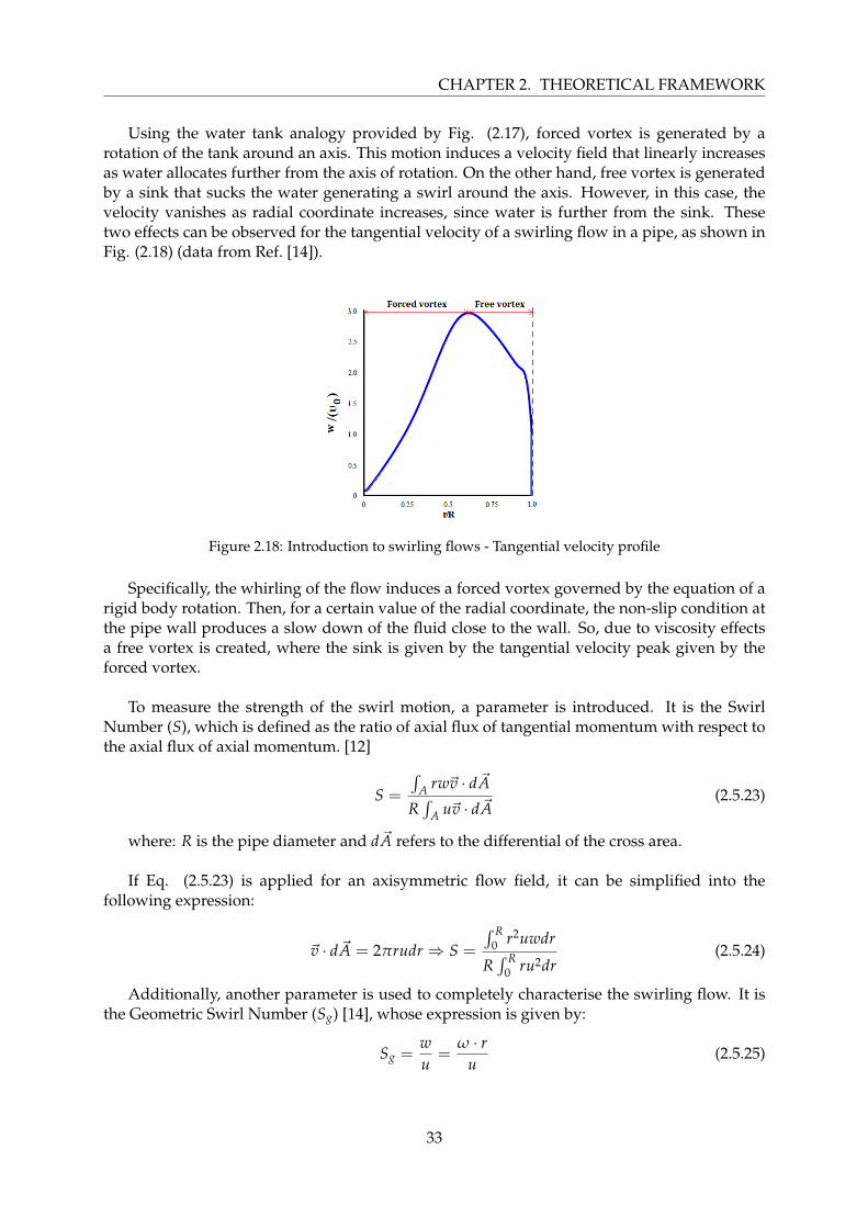
CHAPTER 2. THEORETICAL FRAMEWORK
Using the water tank analogy provided by Fig. (2.17), forced vortex is generated by arotation of the tank around an axis. This motion induces a velocity field that linearly increasesas water allocates further from the axis of rotation. On the other hand, free vortex is generatedby a sink that sucks the water generating a swirl around the axis. However, in this case, thevelocity vanishes as radial coordinate increases, since water is further from the sink. Thesetwo effects can be observed for the tangential velocity of a swirling flow in a pipe, as shown inFig. (2.18) (data from Ref. [14]).
Figure 2.18: Introduction to swirling flows - Tangential velocity profile
Specifically, the whirling of the flow induces a forced vortex governed by the equation of arigid body rotation. Then, for a certain value of the radial coordinate, the non-slip condition atthe pipe wall produces a slow down of the fluid close to the wall. So, due to viscosity effectsa free vortex is created, where the sink is given by the tangential velocity peak given by theforced vortex.
To measure the strength of the swirl motion, a parameter is introduced. It is the SwirlNumber (S), which is defined as the ratio of axial flux of tangential momentum with respect tothe axial flux of axial momentum. [12]
S =
∫A rw~v · d~A
R∫
A u~v · d~A(2.5.23)
where: R is the pipe diameter and d~A refers to the differential of the cross area.
If Eq. (2.5.23) is applied for an axisymmetric flow field, it can be simplified into thefollowing expression:
~v · d~A = 2πrudr ⇒ S =
∫ R0 r2uwdr
R∫ R
0 ru2dr(2.5.24)
Additionally, another parameter is used to completely characterise the swirling flow. It isthe Geometric Swirl Number (Sg) [14], whose expression is given by:
Sg =wu
=ω · r
u(2.5.25)
33
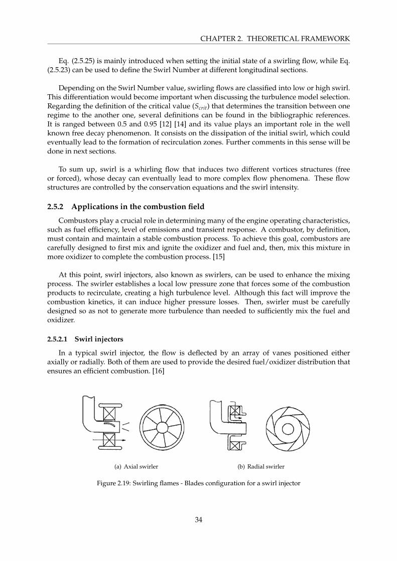
CHAPTER 2. THEORETICAL FRAMEWORK
Eq. (2.5.25) is mainly introduced when setting the initial state of a swirling flow, while Eq.(2.5.23) can be used to define the Swirl Number at different longitudinal sections.
Depending on the Swirl Number value, swirling flows are classified into low or high swirl.This differentiation would become important when discussing the turbulence model selection.Regarding the definition of the critical value (Scrit) that determines the transition between oneregime to the another one, several definitions can be found in the bibliographic references.It is ranged between 0.5 and 0.95 [12] [14] and its value plays an important role in the wellknown free decay phenomenon. It consists on the dissipation of the initial swirl, which couldeventually lead to the formation of recirculation zones. Further comments in this sense will bedone in next sections.
To sum up, swirl is a whirling flow that induces two different vortices structures (freeor forced), whose decay can eventually lead to more complex flow phenomena. These flowstructures are controlled by the conservation equations and the swirl intensity.
2.5.2 Applications in the combustion field
Combustors play a crucial role in determining many of the engine operating characteristics,such as fuel efficiency, level of emissions and transient response. A combustor, by definition,must contain and maintain a stable combustion process. To achieve this goal, combustors arecarefully designed to first mix and ignite the oxidizer and fuel and, then, mix this mixture inmore oxidizer to complete the combustion process. [15]
At this point, swirl injectors, also known as swirlers, can be used to enhance the mixingprocess. The swirler establishes a local low pressure zone that forces some of the combustionproducts to recirculate, creating a high turbulence level. Although this fact will improve thecombustion kinetics, it can induce higher pressure losses. Then, swirler must be carefullydesigned so as not to generate more turbulence than needed to sufficiently mix the fuel andoxidizer.
2.5.2.1 Swirl injectors
In a typical swirl injector, the flow is deflected by an array of vanes positioned eitheraxially or radially. Both of them are used to provide the desired fuel/oxidizer distribution thatensures an efficient combustion. [16]
(a) Axial swirler (b) Radial swirler
Figure 2.19: Swirling flames - Blades configuration for a swirl injector
34
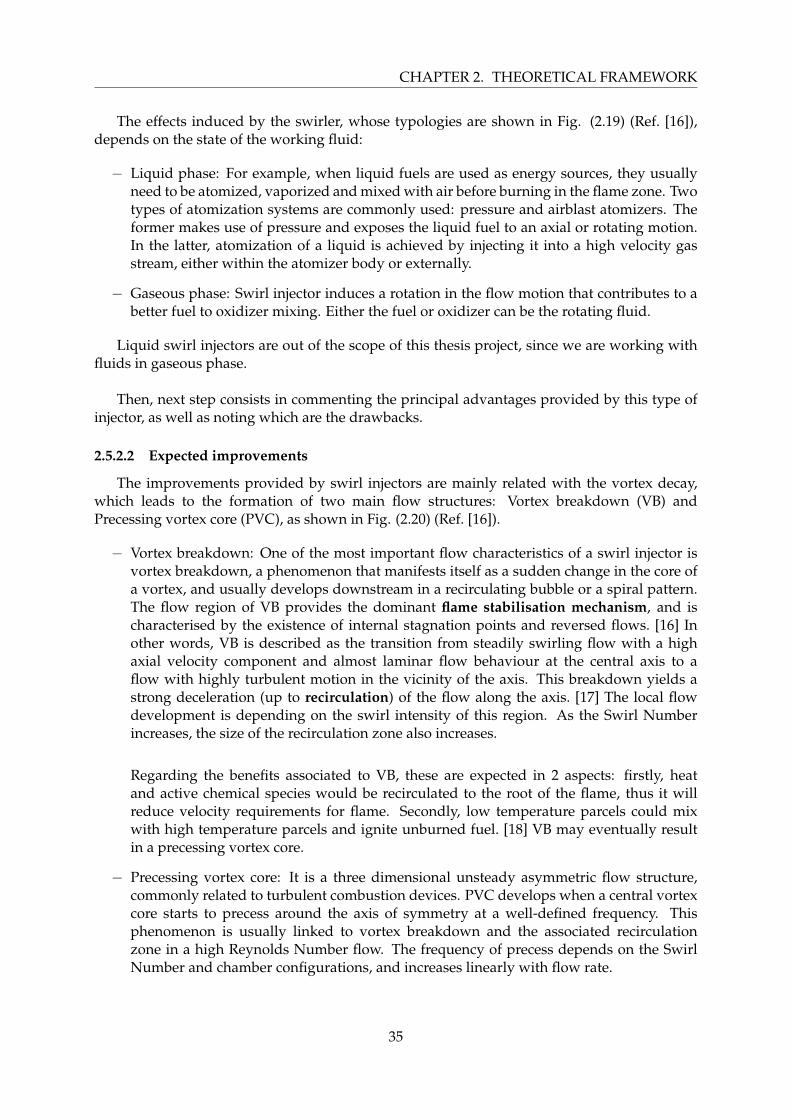
CHAPTER 2. THEORETICAL FRAMEWORK
The effects induced by the swirler, whose typologies are shown in Fig. (2.19) (Ref. [16]),depends on the state of the working fluid:
− Liquid phase: For example, when liquid fuels are used as energy sources, they usuallyneed to be atomized, vaporized and mixed with air before burning in the flame zone. Twotypes of atomization systems are commonly used: pressure and airblast atomizers. Theformer makes use of pressure and exposes the liquid fuel to an axial or rotating motion.In the latter, atomization of a liquid is achieved by injecting it into a high velocity gasstream, either within the atomizer body or externally.
− Gaseous phase: Swirl injector induces a rotation in the flow motion that contributes to abetter fuel to oxidizer mixing. Either the fuel or oxidizer can be the rotating fluid.
Liquid swirl injectors are out of the scope of this thesis project, since we are working withfluids in gaseous phase.
Then, next step consists in commenting the principal advantages provided by this type ofinjector, as well as noting which are the drawbacks.
2.5.2.2 Expected improvements
The improvements provided by swirl injectors are mainly related with the vortex decay,which leads to the formation of two main flow structures: Vortex breakdown (VB) andPrecessing vortex core (PVC), as shown in Fig. (2.20) (Ref. [16]).
− Vortex breakdown: One of the most important flow characteristics of a swirl injector isvortex breakdown, a phenomenon that manifests itself as a sudden change in the core ofa vortex, and usually develops downstream in a recirculating bubble or a spiral pattern.The flow region of VB provides the dominant flame stabilisation mechanism, and ischaracterised by the existence of internal stagnation points and reversed flows. [16] Inother words, VB is described as the transition from steadily swirling flow with a highaxial velocity component and almost laminar flow behaviour at the central axis to aflow with highly turbulent motion in the vicinity of the axis. This breakdown yields astrong deceleration (up to recirculation) of the flow along the axis. [17] The local flowdevelopment is depending on the swirl intensity of this region. As the Swirl Numberincreases, the size of the recirculation zone also increases.
Regarding the benefits associated to VB, these are expected in 2 aspects: firstly, heatand active chemical species would be recirculated to the root of the flame, thus it willreduce velocity requirements for flame. Secondly, low temperature parcels could mixwith high temperature parcels and ignite unburned fuel. [18] VB may eventually resultin a precessing vortex core.
− Precessing vortex core: It is a three dimensional unsteady asymmetric flow structure,commonly related to turbulent combustion devices. PVC develops when a central vortexcore starts to precess around the axis of symmetry at a well-defined frequency. Thisphenomenon is usually linked to vortex breakdown and the associated recirculationzone in a high Reynolds Number flow. The frequency of precess depends on the SwirlNumber and chamber configurations, and increases linearly with flow rate.
35
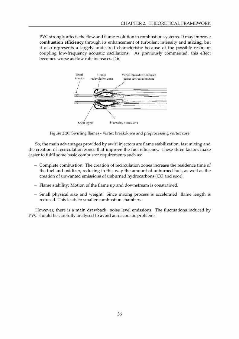
CHAPTER 2. THEORETICAL FRAMEWORK
PVC strongly affects the flow and flame evolution in combustion systems. It may improvecombustion efficiency through its enhancement of turbulent intensity and mixing, butit also represents a largely undesired characteristic because of the possible resonantcoupling low-frequency acoustic oscillations. As previously commented, this effectbecomes worse as flow rate increases. [16]
Figure 2.20: Swirling flames - Vortex breakdown and preprocessing vortex core
So, the main advantages provided by swirl injectors are flame stabilization, fast mixing andthe creation of recirculation zones that improve the fuel efficiency. These three factors makeeasier to fulfil some basic combustor requirements such as:
− Complete combustion: The creation of recirculation zones increase the residence time ofthe fuel and oxidizer, reducing in this way the amount of unburned fuel, as well as thecreation of unwanted emissions of unburned hydrocarbons (CO and soot).
− Flame stability: Motion of the flame up and downstream is constrained.
− Small physical size and weight: Since mixing process is accelerated, flame length isreduced. This leads to smaller combustion chambers.
However, there is a main drawback: noise level emissions. The fluctuations induced byPVC should be carefully analysed to avoid aeroacoustic problems.
36
Chapter 3
Methodology
As already noted in the previous chapter, a computational approach is used to solveturbulent combustion problems. The software used is OpenFoam, whose open source natureallows us implementing new codes in order to solve specific problems. During this work, themain objective is to implement a swirl boundary condition at the inlet. In this way, a swirlinjector is simulated.
So, this chapter explains the basics of a Computational Fluid Dynamics simulation,specifically applied to OpenFOAM environment, as well as describes the implementation ofa swirling flow.
3.1 Computational Fluid Dynamics
Computational Fluid Dynamics is the science that studies the numerical simulation offluid flows. It constitutes an interesting tool because it allows obtaining detailed informationwithout using intrusive experimental measurements. In addition, generally it is cheaper thanperforming its equivalent experiment. [19]
On the other hand, it is difficult to completely control CFD techniques since they requireto have a deep knowledge about fluid dynamics, numerical methods and programming.Complex problems also could be a disadvantage due to the need of a very powerful computer,which is not always possible.
CFD can also be used to construct fluid models that reproduce the behaviour providedby experimental data. This application is the one exploited in this thesis project. Anotherpossibility offered by CFD is to perform parametric analysis in order to design a specificgeometry that provides the most efficient behaviour for a certain field of application.
In what refers to the working principle, a CFD code decompose the fluid domain in cells(mesh), where the conservation equations are solved. When discretising, the partial differentialequations are converted into an algebraic system, which are solved iteratively. In particular,the discretization process adopted for our simulations is the Finite Volume Method (FVM).It is a conservative formulation that sets the conservation equation in integral form for eachcontrol volume (cell).
The stages that define a generic CFD simulation are shown in Fig. (3.1).
37
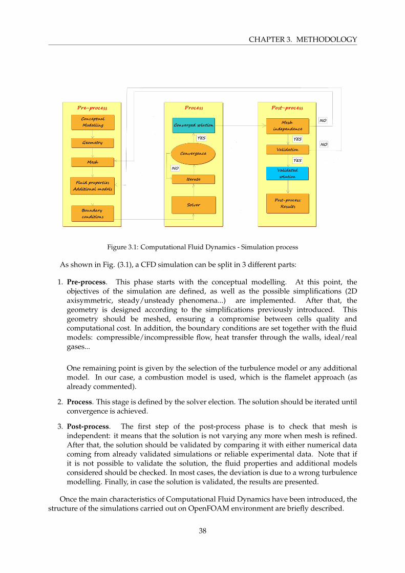
CHAPTER 3. METHODOLOGY
Figure 3.1: Computational Fluid Dynamics - Simulation process
As shown in Fig. (3.1), a CFD simulation can be split in 3 different parts:
1. Pre-process. This phase starts with the conceptual modelling. At this point, theobjectives of the simulation are defined, as well as the possible simplifications (2Daxisymmetric, steady/unsteady phenomena...) are implemented. After that, thegeometry is designed according to the simplifications previously introduced. Thisgeometry should be meshed, ensuring a compromise between cells quality andcomputational cost. In addition, the boundary conditions are set together with the fluidmodels: compressible/incompressible flow, heat transfer through the walls, ideal/realgases...
One remaining point is given by the selection of the turbulence model or any additionalmodel. In our case, a combustion model is used, which is the flamelet approach (asalready commented).
2. Process. This stage is defined by the solver election. The solution should be iterated untilconvergence is achieved.
3. Post-process. The first step of the post-process phase is to check that mesh isindependent: it means that the solution is not varying any more when mesh is refined.After that, the solution should be validated by comparing it with either numerical datacoming from already validated simulations or reliable experimental data. Note that ifit is not possible to validate the solution, the fluid properties and additional modelsconsidered should be checked. In most cases, the deviation is due to a wrong turbulencemodelling. Finally, in case the solution is validated, the results are presented.
Once the main characteristics of Computational Fluid Dynamics have been introduced, thestructure of the simulations carried out on OpenFOAM environment are briefly described.
38
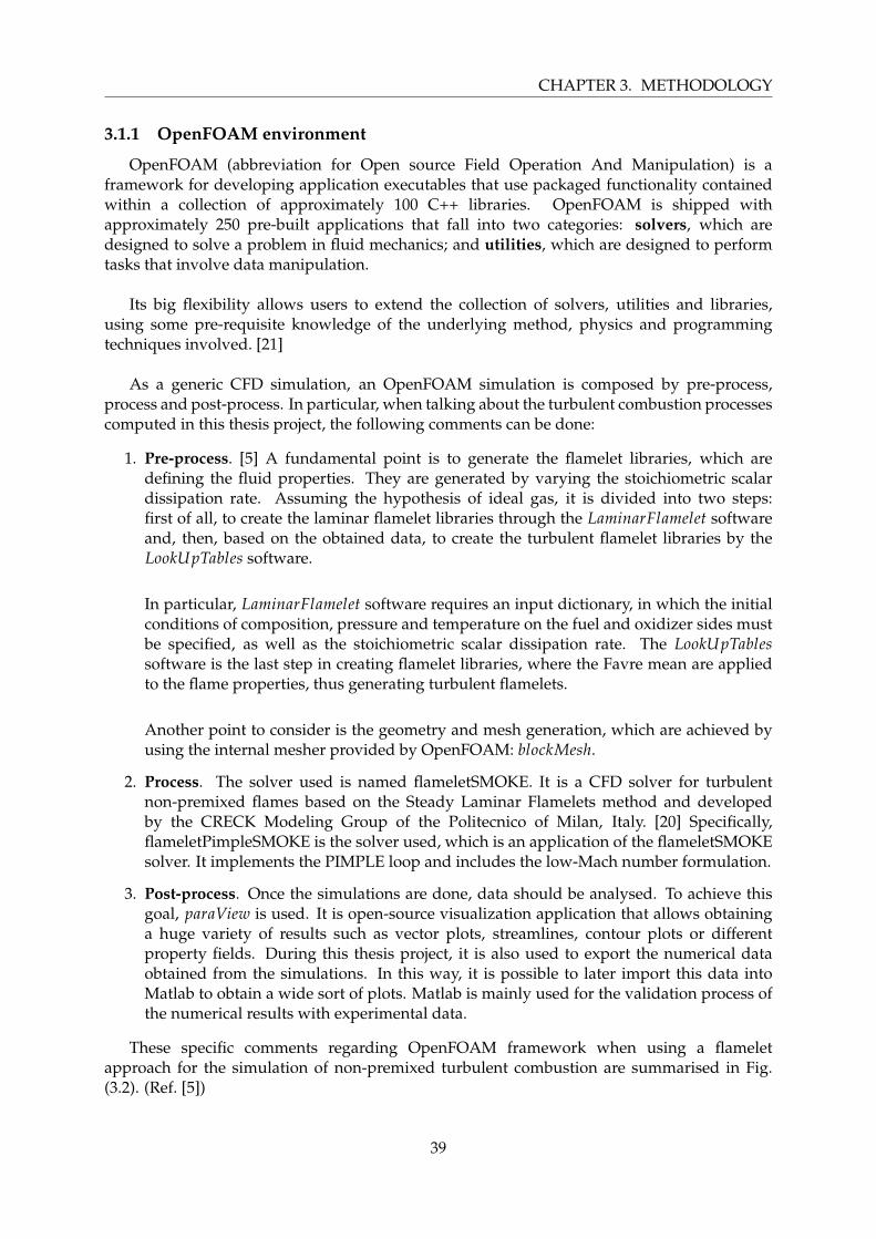
CHAPTER 3. METHODOLOGY
3.1.1 OpenFOAM environment
OpenFOAM (abbreviation for Open source Field Operation And Manipulation) is aframework for developing application executables that use packaged functionality containedwithin a collection of approximately 100 C++ libraries. OpenFOAM is shipped withapproximately 250 pre-built applications that fall into two categories: solvers, which aredesigned to solve a problem in fluid mechanics; and utilities, which are designed to performtasks that involve data manipulation.
Its big flexibility allows users to extend the collection of solvers, utilities and libraries,using some pre-requisite knowledge of the underlying method, physics and programmingtechniques involved. [21]
As a generic CFD simulation, an OpenFOAM simulation is composed by pre-process,process and post-process. In particular, when talking about the turbulent combustion processescomputed in this thesis project, the following comments can be done:
1. Pre-process. [5] A fundamental point is to generate the flamelet libraries, which aredefining the fluid properties. They are generated by varying the stoichiometric scalardissipation rate. Assuming the hypothesis of ideal gas, it is divided into two steps:first of all, to create the laminar flamelet libraries through the LaminarFlamelet softwareand, then, based on the obtained data, to create the turbulent flamelet libraries by theLookUpTables software.
In particular, LaminarFlamelet software requires an input dictionary, in which the initialconditions of composition, pressure and temperature on the fuel and oxidizer sides mustbe specified, as well as the stoichiometric scalar dissipation rate. The LookUpTablessoftware is the last step in creating flamelet libraries, where the Favre mean are appliedto the flame properties, thus generating turbulent flamelets.
Another point to consider is the geometry and mesh generation, which are achieved byusing the internal mesher provided by OpenFOAM: blockMesh.
2. Process. The solver used is named flameletSMOKE. It is a CFD solver for turbulentnon-premixed flames based on the Steady Laminar Flamelets method and developedby the CRECK Modeling Group of the Politecnico of Milan, Italy. [20] Specifically,flameletPimpleSMOKE is the solver used, which is an application of the flameletSMOKEsolver. It implements the PIMPLE loop and includes the low-Mach number formulation.
3. Post-process. Once the simulations are done, data should be analysed. To achieve thisgoal, paraView is used. It is open-source visualization application that allows obtaininga huge variety of results such as vector plots, streamlines, contour plots or differentproperty fields. During this thesis project, it is also used to export the numerical dataobtained from the simulations. In this way, it is possible to later import this data intoMatlab to obtain a wide sort of plots. Matlab is mainly used for the validation process ofthe numerical results with experimental data.
These specific comments regarding OpenFOAM framework when using a flameletapproach for the simulation of non-premixed turbulent combustion are summarised in Fig.(3.2). (Ref. [5])
39
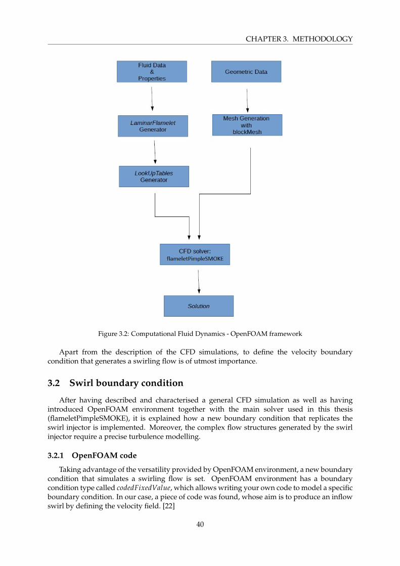
CHAPTER 3. METHODOLOGY
Figure 3.2: Computational Fluid Dynamics - OpenFOAM framework
Apart from the description of the CFD simulations, to define the velocity boundarycondition that generates a swirling flow is of utmost importance.
3.2 Swirl boundary condition
After having described and characterised a general CFD simulation as well as havingintroduced OpenFOAM environment together with the main solver used in this thesis(flameletPimpleSMOKE), it is explained how a new boundary condition that replicates theswirl injector is implemented. Moreover, the complex flow structures generated by the swirlinjector require a precise turbulence modelling.
3.2.1 OpenFOAM code
Taking advantage of the versatility provided by OpenFOAM environment, a new boundarycondition that simulates a swirling flow is set. OpenFOAM environment has a boundarycondition type called codedFixedValue, which allows writing your own code to model a specificboundary condition. In our case, a piece of code was found, whose aim is to produce an inflowswirl by defining the velocity field. [22]
40
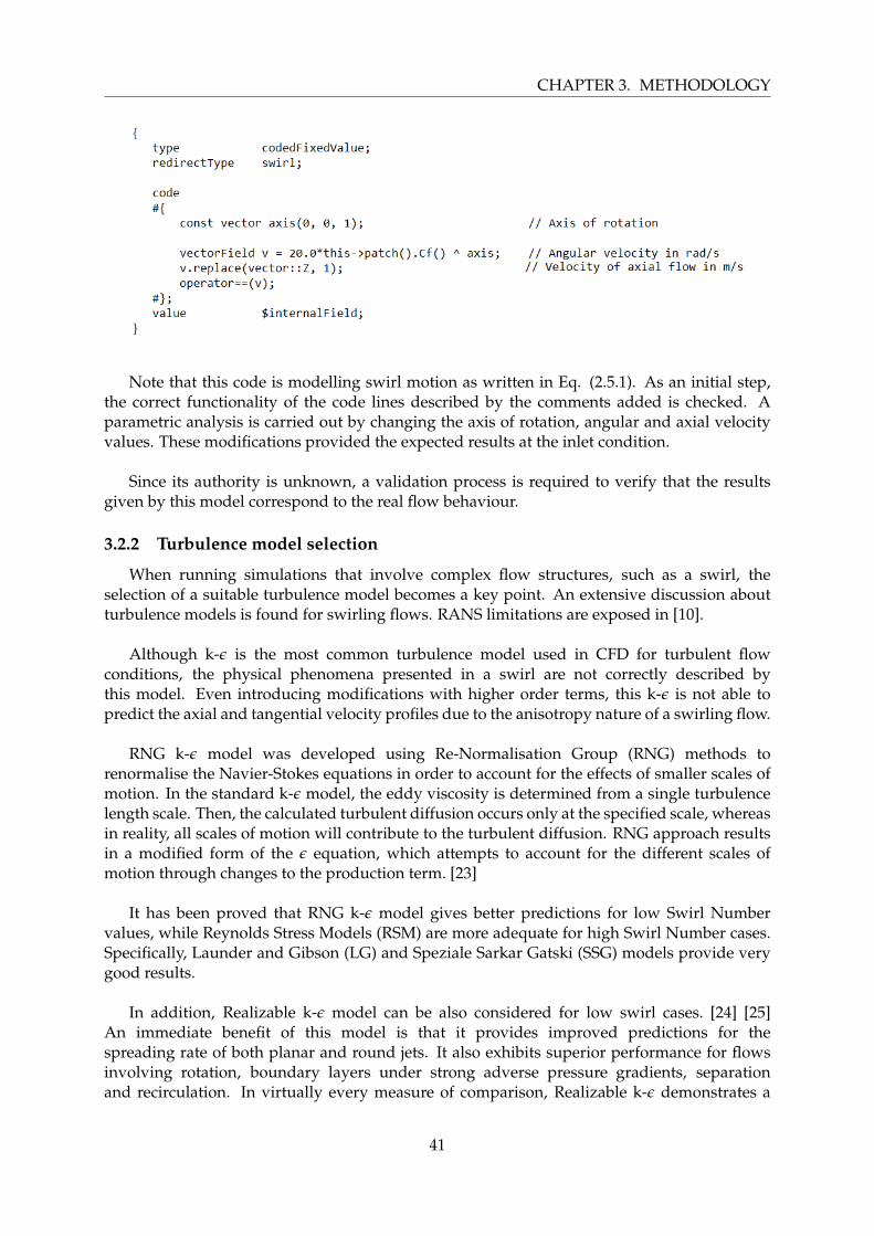
CHAPTER 3. METHODOLOGY
Note that this code is modelling swirl motion as written in Eq. (2.5.1). As an initial step,the correct functionality of the code lines described by the comments added is checked. Aparametric analysis is carried out by changing the axis of rotation, angular and axial velocityvalues. These modifications provided the expected results at the inlet condition.
Since its authority is unknown, a validation process is required to verify that the resultsgiven by this model correspond to the real flow behaviour.
3.2.2 Turbulence model selection
When running simulations that involve complex flow structures, such as a swirl, theselection of a suitable turbulence model becomes a key point. An extensive discussion aboutturbulence models is found for swirling flows. RANS limitations are exposed in [10].
Although k-ε is the most common turbulence model used in CFD for turbulent flowconditions, the physical phenomena presented in a swirl are not correctly described bythis model. Even introducing modifications with higher order terms, this k-ε is not able topredict the axial and tangential velocity profiles due to the anisotropy nature of a swirling flow.
RNG k-ε model was developed using Re-Normalisation Group (RNG) methods torenormalise the Navier-Stokes equations in order to account for the effects of smaller scales ofmotion. In the standard k-ε model, the eddy viscosity is determined from a single turbulencelength scale. Then, the calculated turbulent diffusion occurs only at the specified scale, whereasin reality, all scales of motion will contribute to the turbulent diffusion. RNG approach resultsin a modified form of the ε equation, which attempts to account for the different scales ofmotion through changes to the production term. [23]
It has been proved that RNG k-ε model gives better predictions for low Swirl Numbervalues, while Reynolds Stress Models (RSM) are more adequate for high Swirl Number cases.Specifically, Launder and Gibson (LG) and Speziale Sarkar Gatski (SSG) models provide verygood results.
In addition, Realizable k-ε model can be also considered for low swirl cases. [24] [25]An immediate benefit of this model is that it provides improved predictions for thespreading rate of both planar and round jets. It also exhibits superior performance for flowsinvolving rotation, boundary layers under strong adverse pressure gradients, separationand recirculation. In virtually every measure of comparison, Realizable k-ε demonstrates a
41

CHAPTER 3. METHODOLOGY
superior ability to capture the mean flow of the complex structures.
All these characteristics makes the Realizable k-ε model an optimum choice for low swirlcases.
Moreover, RANS-based RNG k-ε models are compared with LES in [16]. Both LES andRANS are successfully predicting the presence of recirculation zones but they are oversizedby RANS models. This fact leads to a completely different nature of recirculation zones.Regarding the vorticity field, LES shows more fine structure that the RANS result. The RANSonly show the ensemble averaged representative turbulent structures while LES show theturbulent structure solved at grid level. In conclusion, LES results outperform RANS resultsand show a better agreement with the measurements in the statistical results and also betterpredict the flow pattern of the recirculation zones. RANS fails in the modelling of PVC.
Despite the better performance provided by LES, it is decided to use Realizable k-ε modeldue to the computational cost limitations (as pointed out in the previous chapter). In addition,this choice supposes another constraint: only low swirl cases can be studied.
In fact, real applications usually involve low swirled flows to avoid acoustic problems. So,this restriction is not severe. In case it is desired to increase Swirl Number, LES simulationsshould be run to ensure a good description of the turbulence behaviour.
42
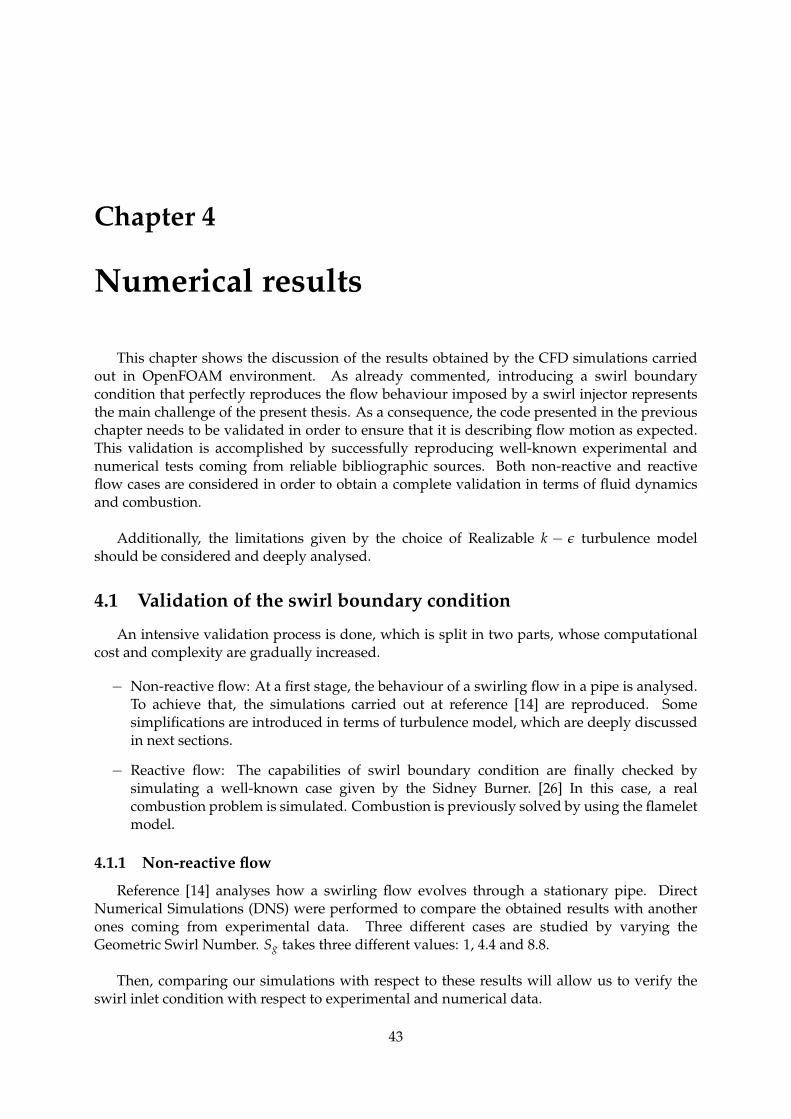
Chapter 4
Numerical results
This chapter shows the discussion of the results obtained by the CFD simulations carriedout in OpenFOAM environment. As already commented, introducing a swirl boundarycondition that perfectly reproduces the flow behaviour imposed by a swirl injector representsthe main challenge of the present thesis. As a consequence, the code presented in the previouschapter needs to be validated in order to ensure that it is describing flow motion as expected.This validation is accomplished by successfully reproducing well-known experimental andnumerical tests coming from reliable bibliographic sources. Both non-reactive and reactiveflow cases are considered in order to obtain a complete validation in terms of fluid dynamicsand combustion.
Additionally, the limitations given by the choice of Realizable k − ε turbulence modelshould be considered and deeply analysed.
4.1 Validation of the swirl boundary condition
An intensive validation process is done, which is split in two parts, whose computationalcost and complexity are gradually increased.
− Non-reactive flow: At a first stage, the behaviour of a swirling flow in a pipe is analysed.To achieve that, the simulations carried out at reference [14] are reproduced. Somesimplifications are introduced in terms of turbulence model, which are deeply discussedin next sections.
− Reactive flow: The capabilities of swirl boundary condition are finally checked bysimulating a well-known case given by the Sidney Burner. [26] In this case, a realcombustion problem is simulated. Combustion is previously solved by using the flameletmodel.
4.1.1 Non-reactive flow
Reference [14] analyses how a swirling flow evolves through a stationary pipe. DirectNumerical Simulations (DNS) were performed to compare the obtained results with anotherones coming from experimental data. Three different cases are studied by varying theGeometric Swirl Number. Sg takes three different values: 1, 4.4 and 8.8.
Then, comparing our simulations with respect to these results will allow us to verify theswirl inlet condition with respect to experimental and numerical data.
43
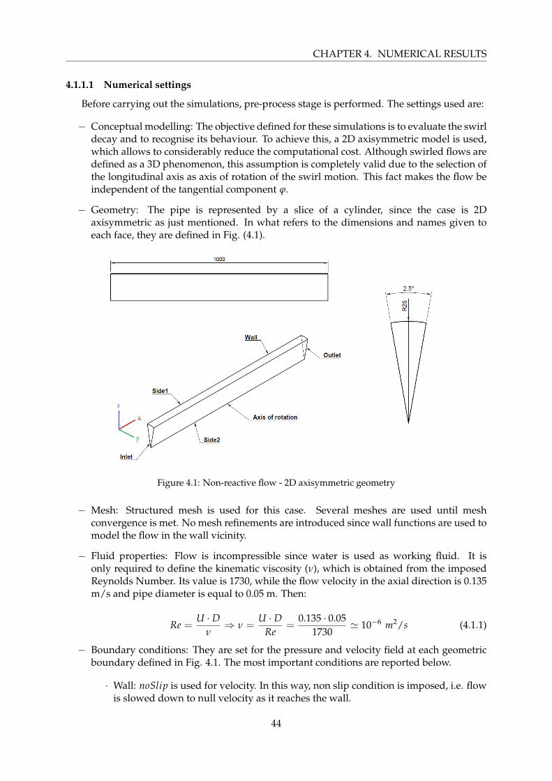
CHAPTER 4. NUMERICAL RESULTS
4.1.1.1 Numerical settings
Before carrying out the simulations, pre-process stage is performed. The settings used are:
− Conceptual modelling: The objective defined for these simulations is to evaluate the swirldecay and to recognise its behaviour. To achieve this, a 2D axisymmetric model is used,which allows to considerably reduce the computational cost. Although swirled flows aredefined as a 3D phenomenon, this assumption is completely valid due to the selection ofthe longitudinal axis as axis of rotation of the swirl motion. This fact makes the flow beindependent of the tangential component ϕ.
− Geometry: The pipe is represented by a slice of a cylinder, since the case is 2Daxisymmetric as just mentioned. In what refers to the dimensions and names given toeach face, they are defined in Fig. (4.1).
Figure 4.1: Non-reactive flow - 2D axisymmetric geometry
− Mesh: Structured mesh is used for this case. Several meshes are used until meshconvergence is met. No mesh refinements are introduced since wall functions are used tomodel the flow in the wall vicinity.
− Fluid properties: Flow is incompressible since water is used as working fluid. It isonly required to define the kinematic viscosity (ν), which is obtained from the imposedReynolds Number. Its value is 1730, while the flow velocity in the axial direction is 0.135m/s and pipe diameter is equal to 0.05 m. Then:
Re =U · D
ν⇒ ν =
U · DRe
=0.135 · 0.05
1730' 10−6 m2/s (4.1.1)
− Boundary conditions: They are set for the pressure and velocity field at each geometricboundary defined in Fig. 4.1. The most important conditions are reported below.
· Wall: noSlip is used for velocity. In this way, non slip condition is imposed, i.e. flowis slowed down to null velocity as it reaches the wall.
44
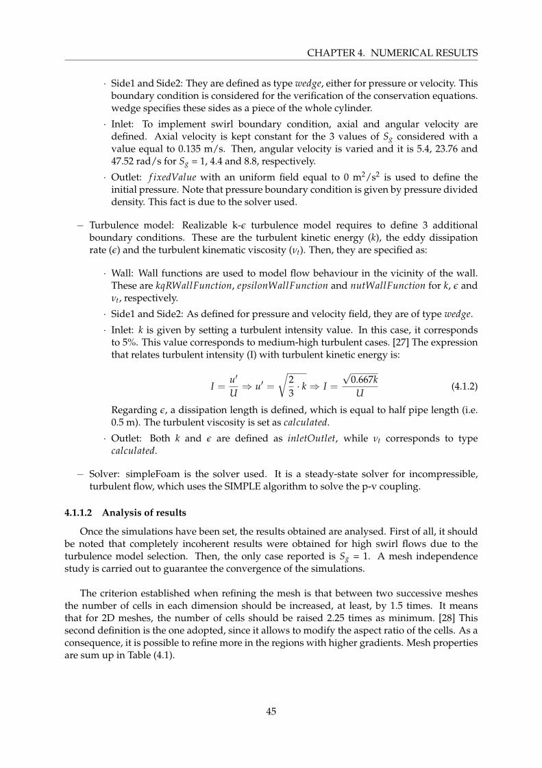
CHAPTER 4. NUMERICAL RESULTS
· Side1 and Side2: They are defined as type wedge, either for pressure or velocity. Thisboundary condition is considered for the verification of the conservation equations.wedge specifies these sides as a piece of the whole cylinder.
· Inlet: To implement swirl boundary condition, axial and angular velocity aredefined. Axial velocity is kept constant for the 3 values of Sg considered with avalue equal to 0.135 m/s. Then, angular velocity is varied and it is 5.4, 23.76 and47.52 rad/s for Sg = 1, 4.4 and 8.8, respectively.
· Outlet: f ixedValue with an uniform field equal to 0 m2/s2 is used to define theinitial pressure. Note that pressure boundary condition is given by pressure divideddensity. This fact is due to the solver used.
− Turbulence model: Realizable k-ε turbulence model requires to define 3 additionalboundary conditions. These are the turbulent kinetic energy (k), the eddy dissipationrate (ε) and the turbulent kinematic viscosity (νt). Then, they are specified as:
· Wall: Wall functions are used to model flow behaviour in the vicinity of the wall.These are kqRWallFunction, epsilonWallFunction and nutWallFunction for k, ε andνt, respectively.
· Side1 and Side2: As defined for pressure and velocity field, they are of type wedge.
· Inlet: k is given by setting a turbulent intensity value. In this case, it correspondsto 5%. This value corresponds to medium-high turbulent cases. [27] The expressionthat relates turbulent intensity (I) with turbulent kinetic energy is:
I =u′
U⇒ u′ =
√23· k⇒ I =
√0.667k
U(4.1.2)
Regarding ε, a dissipation length is defined, which is equal to half pipe length (i.e.0.5 m). The turbulent viscosity is set as calculated.
· Outlet: Both k and ε are defined as inletOutlet, while νt corresponds to typecalculated.
− Solver: simpleFoam is the solver used. It is a steady-state solver for incompressible,turbulent flow, which uses the SIMPLE algorithm to solve the p-v coupling.
4.1.1.2 Analysis of results
Once the simulations have been set, the results obtained are analysed. First of all, it shouldbe noted that completely incoherent results were obtained for high swirl flows due to theturbulence model selection. Then, the only case reported is Sg = 1. A mesh independencestudy is carried out to guarantee the convergence of the simulations.
The criterion established when refining the mesh is that between two successive meshesthe number of cells in each dimension should be increased, at least, by 1.5 times. It meansthat for 2D meshes, the number of cells should be raised 2.25 times as minimum. [28] Thissecond definition is the one adopted, since it allows to modify the aspect ratio of the cells. As aconsequence, it is possible to refine more in the regions with higher gradients. Mesh propertiesare sum up in Table (4.1).
45
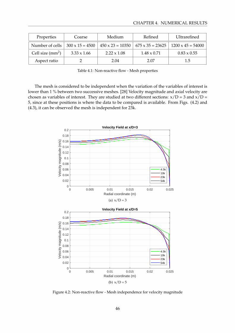
CHAPTER 4. NUMERICAL RESULTS
Properties Coarse Medium Refined Ultrarefined
Number of cells 300 x 15 = 4500 450 x 23 = 10350 675 x 35 = 23625 1200 x 45 = 54000
Cell size (mm2) 3.33 x 1.66 2.22 x 1.08 1.48 x 0.71 0.83 x 0.55
Aspect ratio 2 2.04 2.07 1.5
Table 4.1: Non-reactive flow - Mesh properties
The mesh is considered to be independent when the variation of the variables of interest islower than 1 % between two successive meshes. [28] Velocity magnitude and axial velocity arechosen as variables of interest. They are studied at two different sections: x/D = 3 and x/D =5, since at these positions is where the data to be compared is available. From Figs. (4.2) and(4.3), it can be observed the mesh is independent for 23k.
0 0.005 0.01 0.015 0.02 0.025
Radial coordinate (m)
0
0.02
0.04
0.06
0.08
0.1
0.12
0.14
0.16
0.18
0.2
Vel
ocity
mag
nitu
de (
m/s
)
Velocity Field at x/D=3
4.5k10k23k54k
(a) x/D = 3
0 0.005 0.01 0.015 0.02 0.025
Radial coordinate (m)
0
0.02
0.04
0.06
0.08
0.1
0.12
0.14
0.16
0.18
0.2
Vel
ocity
mag
nitu
de (
m/s
)
Velocity Field at x/D=5
4.5k10k23k54k
(b) x/D = 5
Figure 4.2: Non-reactive flow - Mesh independence for velocity magnitude
46
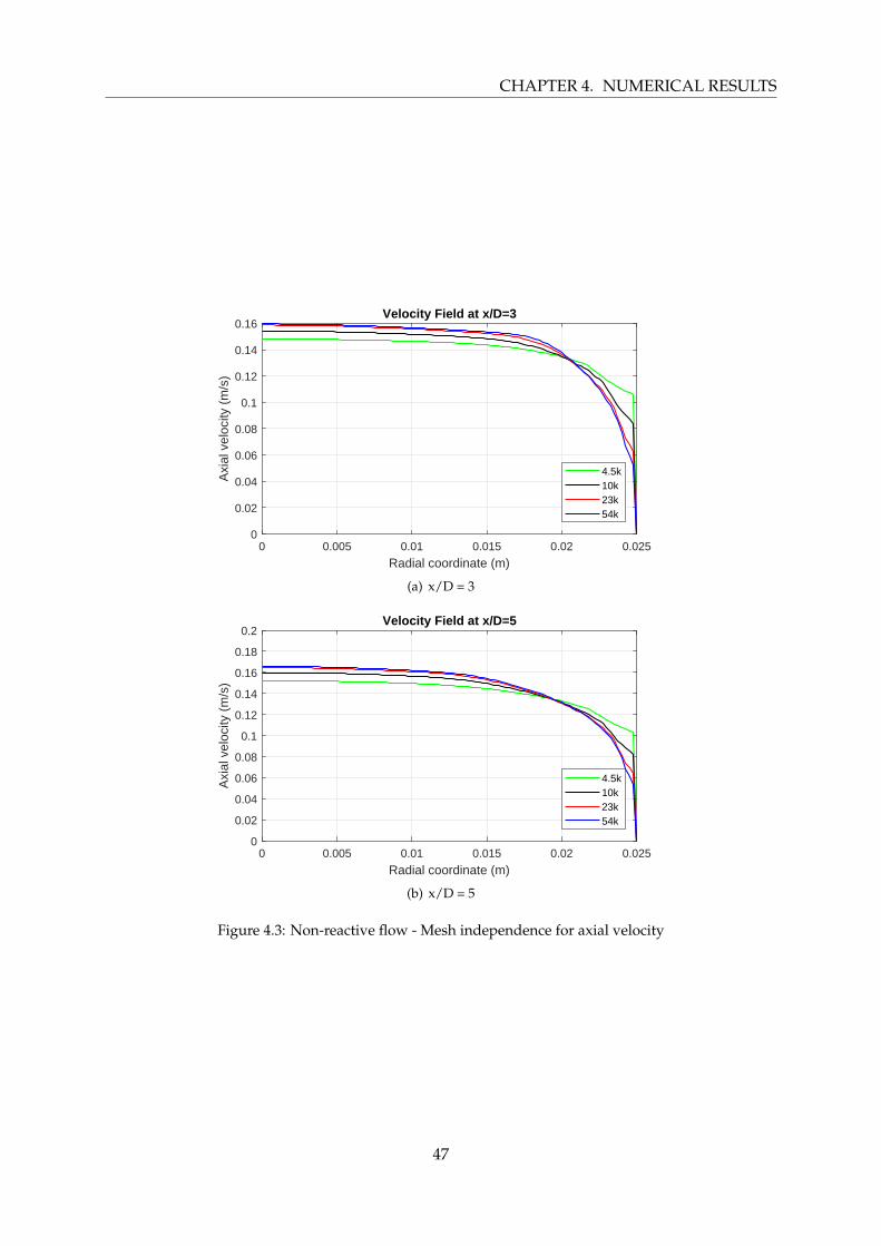
CHAPTER 4. NUMERICAL RESULTS
0 0.005 0.01 0.015 0.02 0.025
Radial coordinate (m)
0
0.02
0.04
0.06
0.08
0.1
0.12
0.14
0.16
Axi
al v
eloc
ity (
m/s
)
Velocity Field at x/D=3
4.5k10k23k54k
(a) x/D = 3
0 0.005 0.01 0.015 0.02 0.025
Radial coordinate (m)
0
0.02
0.04
0.06
0.08
0.1
0.12
0.14
0.16
0.18
0.2
Axi
al v
eloc
ity (
m/s
)
Velocity Field at x/D=5
4.5k10k23k54k
(b) x/D = 5
Figure 4.3: Non-reactive flow - Mesh independence for axial velocity
47
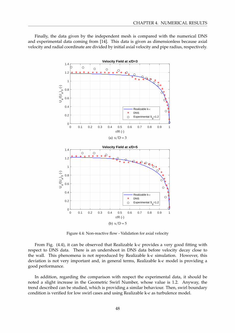
CHAPTER 4. NUMERICAL RESULTS
Finally, the data given by the independent mesh is compared with the numerical DNSand experimental data coming from [14]. This data is given as dimensionless because axialvelocity and radial coordinate are divided by initial axial velocity and pipe radius, respectively.
0 0.1 0.2 0.3 0.4 0.5 0.6 0.7 0.8 0.9 1
r/R (-)
0
0.2
0.4
0.6
0.8
1
1.2
1.4U
a/(
Ua) 0
(-)
Velocity Field at x/D=3
Realizable k-DNSExperimental S
g=1.2
(a) x/D = 3
0 0.1 0.2 0.3 0.4 0.5 0.6 0.7 0.8 0.9 1
r/R (-)
0
0.2
0.4
0.6
0.8
1
1.2
1.4
Ua/(
Ua) 0
(-)
Velocity Field at x/D=5
Realizable k-DNSExperimental S
g=1.2
(b) x/D = 5
Figure 4.4: Non-reactive flow - Validation for axial velocity
From Fig. (4.4), it can be observed that Realizable k-ε provides a very good fitting withrespect to DNS data. There is an undershoot in DNS data before velocity decay close tothe wall. This phenomena is not reproduced by Realizable k-ε simulation. However, thisdeviation is not very important and, in general terms, Realizable k-ε model is providing agood performance.
In addition, regarding the comparison with respect the experimental data, it should benoted a slight increase in the Geometric Swirl Number, whose value is 1.2. Anyway, thetrend described can be studied, which is providing a similar behaviour. Then, swirl boundarycondition is verified for low swirl cases and using Realizable k-ε as turbulence model.
48
CHAPTER 4. NUMERICAL RESULTS
4.1.2 Non-reactive flow by flamelet model
Before running the reactive flow simulations, which make of use the flamelet modelto compute the flow properties coming from the combustion process, another simulationinvolving non-reactive flow is done. Flamelet model is introduced for calculating the flowproperties of a non-reactive flow. It means that constant properties are found for any mixturefraction since only one fluid is used (H2O in liquid phase). In this way, instead of definingthe fluid properties at transportProperties file, they are defined through the generated flameletlibrary, which is called when running flameletSMOKE solvers.
4.1.2.1 Numerical settings
The pre-process is almost equal to the one previously set for simpleFoam simulation.The changes performed are linked to the new solver, which is flameletPimpleSMOKE. Itsolves the p-v coupling by using the PIMPLE algorithm and it asks for the fluid propertiesto the generated flamelet library. Regarding the numerical settings, the main modificationsintroduced are:
− Fluid properties: As already noted, fluid properties are loaded from the flamelet library,whose path is defined in f lameletProperties file. Flamelet libraries are composed by 11thermodynamic properties. These are the mixture fraction (Z), temperature (T), pressure(p), molecular weight (Mw), density (ρ), scalar dissipation rate (χ), enthalpy (h), isobaricheat capacity (cp), thermal conductivity (λ), thermal diffusivity (α) and dynamic viscosity(µ). Note that all these properties are the turbulent ones, and not the laminar ones.
Additionally, n mass fractions corresponding to the n elements that compound themixture. In this case, there is only one specie: H2O. In the previous simulation(simpleFoam), the only fluid property defined was the kinematic viscosity. However,in this case, it is defined the dynamic viscosity and the density, in such a way that itsquotient leads to the same value for ν.
− Boundary conditions: flameletPimpleSMOKE solver requires to define 11 boundaryconditions. This fact means that 6 additional properties are introduced with respect tosimpleFoam simulation. These are the turbulent thermal diffusivity (αt), enthalpy (h),turbulent dynamic viscosity (µt), temperature (T), mixture fraction (Z) and its variance(Zvar). They are defined in correspondence to the values contained in the flamelet library.
Moreover, it should be pointed out that the actual pressure should be set in thissimulation, which is equal to 1 atmosphere.
In what refers to the domain discretization, the independent mesh found in simpleFoamsimulation is used. Then, once the setting is completed, the simulation is carried out.
4.1.2.2 Analysis of results
The results obtained with flameletPimpleSMOKE solver are compared with the ones givenby simpleFoam solver. This comparison is performed for velocity magnitude and axialvelocity, as shown in Figs. (4.5) and (4.6). It can be observed a perfect overlapping betweensimpleFoam and flameletPimpleSMOKE curves. As a consequence, flameletPimpleSMOKEsolver is validated for swirling non reactive flows.
49
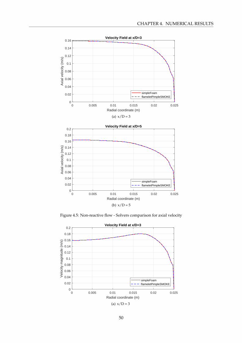
CHAPTER 4. NUMERICAL RESULTS
0 0.005 0.01 0.015 0.02 0.025
Radial coordinate (m)
0
0.02
0.04
0.06
0.08
0.1
0.12
0.14
0.16
Axi
al v
eloc
ity (
m/s
)
Velocity Field at x/D=3
simpleFoamflameletPimpleSMOKE
(a) x/D = 3
0 0.005 0.01 0.015 0.02 0.025
Radial coordinate (m)
0
0.02
0.04
0.06
0.08
0.1
0.12
0.14
0.16
0.18
0.2
Axi
al v
eloc
ity (
m/s
)
Velocity Field at x/D=5
simpleFoamflameletPimpleSMOKE
(b) x/D = 5
Figure 4.5: Non-reactive flow - Solvers comparison for axial velocity
0 0.005 0.01 0.015 0.02 0.025
Radial coordinate (m)
0
0.02
0.04
0.06
0.08
0.1
0.12
0.14
0.16
0.18
0.2
Vel
ocity
mag
nitu
de (
m/s
)
Velocity Field at x/D=3
simpleFoamflameletPimpleSMOKE
(a) x/D = 3
50
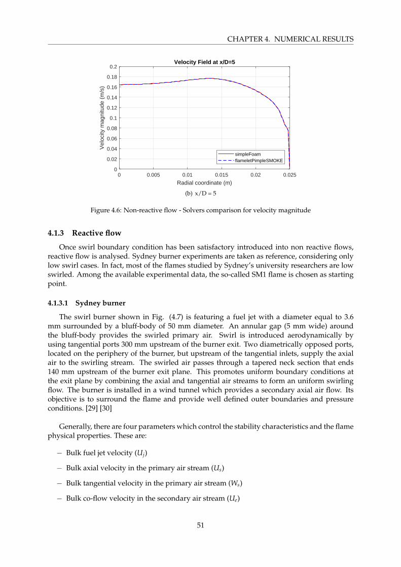
CHAPTER 4. NUMERICAL RESULTS
0 0.005 0.01 0.015 0.02 0.025
Radial coordinate (m)
0
0.02
0.04
0.06
0.08
0.1
0.12
0.14
0.16
0.18
0.2
Vel
ocity
mag
nitu
de (
m/s
)
Velocity Field at x/D=5
simpleFoamflameletPimpleSMOKE
(b) x/D = 5
Figure 4.6: Non-reactive flow - Solvers comparison for velocity magnitude
4.1.3 Reactive flow
Once swirl boundary condition has been satisfactory introduced into non reactive flows,reactive flow is analysed. Sydney burner experiments are taken as reference, considering onlylow swirl cases. In fact, most of the flames studied by Sydney’s university researchers are lowswirled. Among the available experimental data, the so-called SM1 flame is chosen as startingpoint.
4.1.3.1 Sydney burner
The swirl burner shown in Fig. (4.7) is featuring a fuel jet with a diameter equal to 3.6mm surrounded by a bluff-body of 50 mm diameter. An annular gap (5 mm wide) aroundthe bluff-body provides the swirled primary air. Swirl is introduced aerodynamically byusing tangential ports 300 mm upstream of the burner exit. Two diametrically opposed ports,located on the periphery of the burner, but upstream of the tangential inlets, supply the axialair to the swirling stream. The swirled air passes through a tapered neck section that ends140 mm upstream of the burner exit plane. This promotes uniform boundary conditions atthe exit plane by combining the axial and tangential air streams to form an uniform swirlingflow. The burner is installed in a wind tunnel which provides a secondary axial air flow. Itsobjective is to surround the flame and provide well defined outer boundaries and pressureconditions. [29] [30]
Generally, there are four parameters which control the stability characteristics and the flamephysical properties. These are:
− Bulk fuel jet velocity (Uj)
− Bulk axial velocity in the primary air stream (Us)
− Bulk tangential velocity in the primary air stream (Ws)
− Bulk co-flow velocity in the secondary air stream (Ue)
51
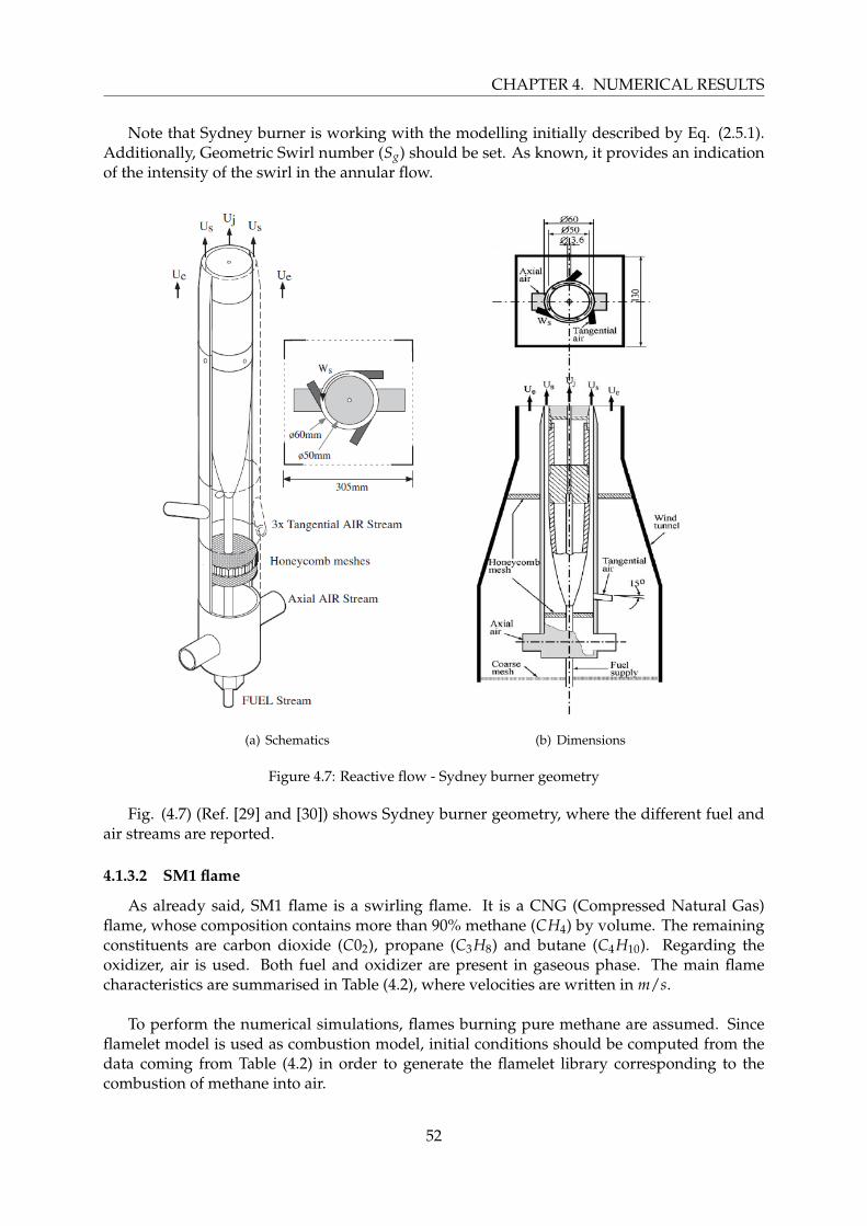
CHAPTER 4. NUMERICAL RESULTS
Note that Sydney burner is working with the modelling initially described by Eq. (2.5.1).Additionally, Geometric Swirl number (Sg) should be set. As known, it provides an indicationof the intensity of the swirl in the annular flow.
(a) Schematics (b) Dimensions
Figure 4.7: Reactive flow - Sydney burner geometry
Fig. (4.7) (Ref. [29] and [30]) shows Sydney burner geometry, where the different fuel andair streams are reported.
4.1.3.2 SM1 flame
As already said, SM1 flame is a swirling flame. It is a CNG (Compressed Natural Gas)flame, whose composition contains more than 90% methane (CH4) by volume. The remainingconstituents are carbon dioxide (C02), propane (C3H8) and butane (C4H10). Regarding theoxidizer, air is used. Both fuel and oxidizer are present in gaseous phase. The main flamecharacteristics are summarised in Table (4.2), where velocities are written in m/s.
To perform the numerical simulations, flames burning pure methane are assumed. Sinceflamelet model is used as combustion model, initial conditions should be computed from thedata coming from Table (4.2) in order to generate the flamelet library corresponding to thecombustion of methane into air.
52
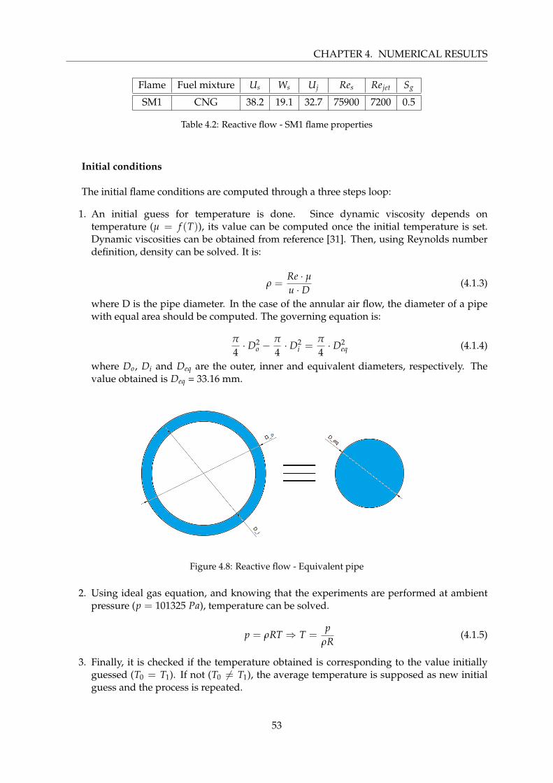
CHAPTER 4. NUMERICAL RESULTS
Flame Fuel mixture Us Ws Uj Res Rejet Sg
SM1 CNG 38.2 19.1 32.7 75900 7200 0.5
Table 4.2: Reactive flow - SM1 flame properties
Initial conditions
The initial flame conditions are computed through a three steps loop:
1. An initial guess for temperature is done. Since dynamic viscosity depends ontemperature (µ = f (T)), its value can be computed once the initial temperature is set.Dynamic viscosities can be obtained from reference [31]. Then, using Reynolds numberdefinition, density can be solved. It is:
ρ =Re · µu · D (4.1.3)
where D is the pipe diameter. In the case of the annular air flow, the diameter of a pipewith equal area should be computed. The governing equation is:
π
4· D2
o −π
4· D2
i =π
4· D2
eq (4.1.4)
where Do, Di and Deq are the outer, inner and equivalent diameters, respectively. Thevalue obtained is Deq = 33.16 mm.
Figure 4.8: Reactive flow - Equivalent pipe
2. Using ideal gas equation, and knowing that the experiments are performed at ambientpressure (p = 101325 Pa), temperature can be solved.
p = ρRT ⇒ T =p
ρR(4.1.5)
3. Finally, it is checked if the temperature obtained is corresponding to the value initiallyguessed (T0 = T1). If not (T0 6= T1), the average temperature is supposed as new initialguess and the process is repeated.
53
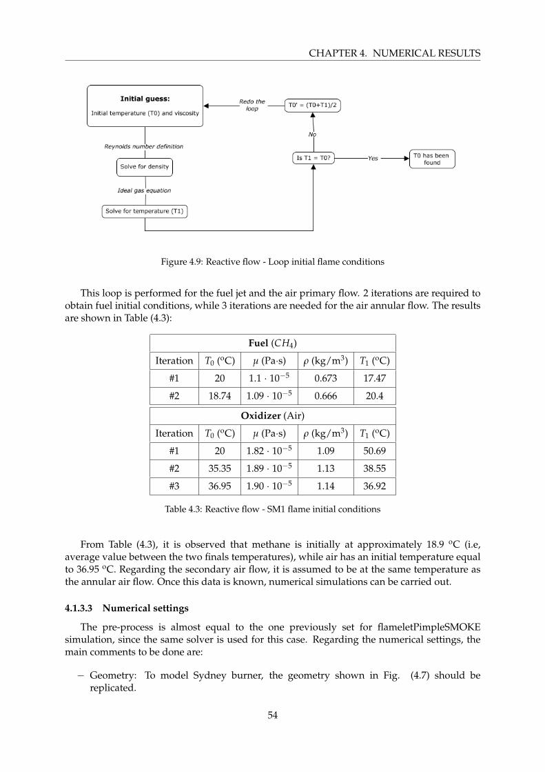
CHAPTER 4. NUMERICAL RESULTS
Figure 4.9: Reactive flow - Loop initial flame conditions
This loop is performed for the fuel jet and the air primary flow. 2 iterations are required toobtain fuel initial conditions, while 3 iterations are needed for the air annular flow. The resultsare shown in Table (4.3):
Fuel (CH4)
Iteration T0 (oC) µ (Pa·s) ρ (kg/m3) T1 (oC)
#1 20 1.1 · 10−5 0.673 17.47
#2 18.74 1.09 · 10−5 0.666 20.4
Oxidizer (Air)
Iteration T0 (oC) µ (Pa·s) ρ (kg/m3) T1 (oC)
#1 20 1.82 · 10−5 1.09 50.69
#2 35.35 1.89 · 10−5 1.13 38.55
#3 36.95 1.90 · 10−5 1.14 36.92
Table 4.3: Reactive flow - SM1 flame initial conditions
From Table (4.3), it is observed that methane is initially at approximately 18.9 oC (i.e,average value between the two finals temperatures), while air has an initial temperature equalto 36.95 oC. Regarding the secondary air flow, it is assumed to be at the same temperature asthe annular air flow. Once this data is known, numerical simulations can be carried out.
4.1.3.3 Numerical settings
The pre-process is almost equal to the one previously set for flameletPimpleSMOKEsimulation, since the same solver is used for this case. Regarding the numerical settings, themain comments to be done are:
− Geometry: To model Sydney burner, the geometry shown in Fig. (4.7) should bereplicated.
54
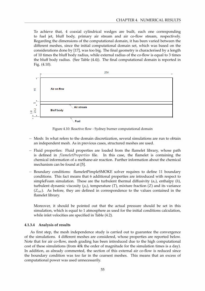
CHAPTER 4. NUMERICAL RESULTS
To achieve that, 4 coaxial cylindrical wedges are built, each one correspondingto fuel jet, bluff body, primary air stream and air co-flow stream, respectively.Regarding the dimensions of the computational domain, it has been varied between thedifferent meshes, since the initial computational domain set, which was based on theconsiderations done by [17], was too big. The final geometry is characterised by a lengthof 10 times the bluff body radius, while external radius of the co-flow is equal to 3 timesthe bluff body radius. (See Table (4.4)). The final computational domain is reported inFig. (4.10).
Figure 4.10: Reactive flow - Sydney burner computational domain
− Mesh: In what refers to the domain discretization, several simulations are run to obtainan independent mesh. As in previous cases, structured meshes are used.
− Fluid properties: Fluid properties are loaded from the flamelet library, whose pathis defined in f lameletProperties file. In this case, the flamelet is containing thechemical information of a methane-air reaction. Further information about the chemicalmechanism can be found at [5].
− Boundary conditions: flameletPimpleSMOKE solver requires to define 11 boundaryconditions. This fact means that 6 additional properties are introduced with respect tosimpleFoam simulation. These are the turbulent thermal diffusivity (αt), enthalpy (h),turbulent dynamic viscosity (µt), temperature (T), mixture fraction (Z) and its variance(Zvar). As before, they are defined in correspondence to the values contained in theflamelet library.
Moreover, it should be pointed out that the actual pressure should be set in thissimulation, which is equal to 1 atmosphere as used for the initial conditions calculation,while inlet velocities are specified in Table (4.2).
4.1.3.4 Analysis of results
As first step, the mesh independence study is carried out to guarantee the convergenceof the simulations. 4 different meshes are considered, whose properties are reported below.Note that for air co-flow, mesh grading has been introduced due to the high computationalcost of these simulations (from 40k the order of magnitude for the simulation times is a day).In addition, as already commented, the section of this external air co-flow is reduced sincethe boundary condition was too far in the coarsest meshes. This means that an excess ofcomputational power was used unnecessarily.
55
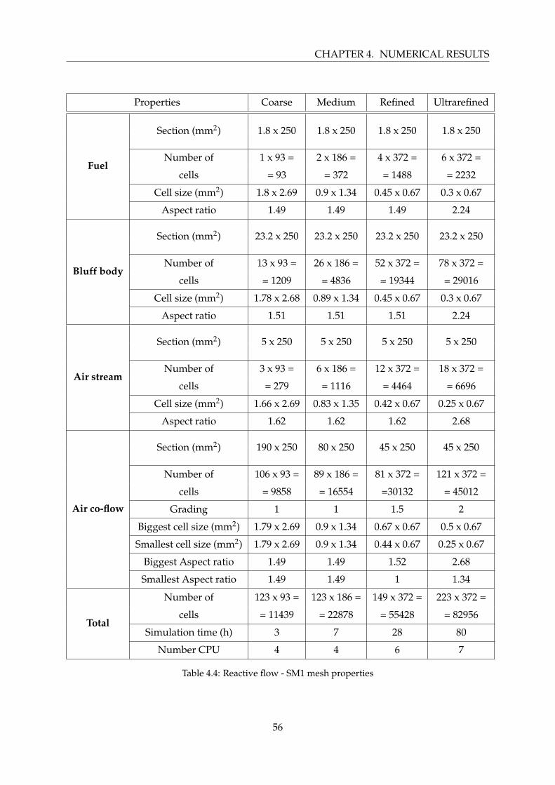
CHAPTER 4. NUMERICAL RESULTS
Properties Coarse Medium Refined Ultrarefined
Fuel
Section (mm2) 1.8 x 250 1.8 x 250 1.8 x 250 1.8 x 250
Number of 1 x 93 = 2 x 186 = 4 x 372 = 6 x 372 =
cells = 93 = 372 = 1488 = 2232
Cell size (mm2) 1.8 x 2.69 0.9 x 1.34 0.45 x 0.67 0.3 x 0.67
Aspect ratio 1.49 1.49 1.49 2.24
Bluff body
Section (mm2) 23.2 x 250 23.2 x 250 23.2 x 250 23.2 x 250
Number of 13 x 93 = 26 x 186 = 52 x 372 = 78 x 372 =
cells = 1209 = 4836 = 19344 = 29016
Cell size (mm2) 1.78 x 2.68 0.89 x 1.34 0.45 x 0.67 0.3 x 0.67
Aspect ratio 1.51 1.51 1.51 2.24
Air stream
Section (mm2) 5 x 250 5 x 250 5 x 250 5 x 250
Number of 3 x 93 = 6 x 186 = 12 x 372 = 18 x 372 =
cells = 279 = 1116 = 4464 = 6696
Cell size (mm2) 1.66 x 2.69 0.83 x 1.35 0.42 x 0.67 0.25 x 0.67
Aspect ratio 1.62 1.62 1.62 2.68
Air co-flow
Section (mm2) 190 x 250 80 x 250 45 x 250 45 x 250
Number of 106 x 93 = 89 x 186 = 81 x 372 = 121 x 372 =
cells = 9858 = 16554 =30132 = 45012
Grading 1 1 1.5 2
Biggest cell size (mm2) 1.79 x 2.69 0.9 x 1.34 0.67 x 0.67 0.5 x 0.67
Smallest cell size (mm2) 1.79 x 2.69 0.9 x 1.34 0.44 x 0.67 0.25 x 0.67
Biggest Aspect ratio 1.49 1.49 1.52 2.68
Smallest Aspect ratio 1.49 1.49 1 1.34
Total
Number of 123 x 93 = 123 x 186 = 149 x 372 = 223 x 372 =
cells = 11439 = 22878 = 55428 = 82956
Simulation time (h) 3 7 28 80
Number CPU 4 4 6 7
Table 4.4: Reactive flow - SM1 mesh properties
56
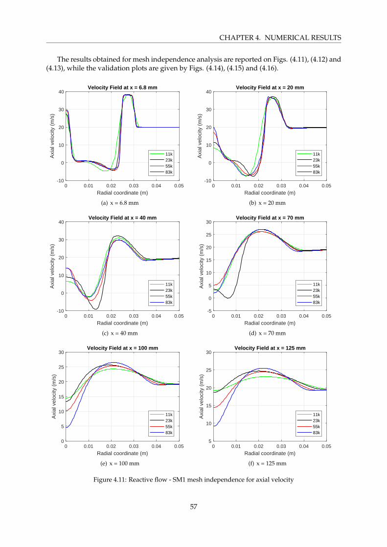
CHAPTER 4. NUMERICAL RESULTS
The results obtained for mesh independence analysis are reported on Figs. (4.11), (4.12) and(4.13), while the validation plots are given by Figs. (4.14), (4.15) and (4.16).
0 0.01 0.02 0.03 0.04 0.05
Radial coordinate (m)
-10
0
10
20
30
40
Axi
al v
eloc
ity (
m/s
)
Velocity Field at x = 6.8 mm
11k23k55k83k
(a) x = 6.8 mm
0 0.01 0.02 0.03 0.04 0.05
Radial coordinate (m)
-10
0
10
20
30
40
Axi
al v
eloc
ity (
m/s
)
Velocity Field at x = 20 mm
11k23k55k83k
(b) x = 20 mm
0 0.01 0.02 0.03 0.04 0.05
Radial coordinate (m)
-10
0
10
20
30
40
Axi
al v
eloc
ity (
m/s
)
Velocity Field at x = 40 mm
11k23k55k83k
(c) x = 40 mm
0 0.01 0.02 0.03 0.04 0.05
Radial coordinate (m)
-5
0
5
10
15
20
25
30
Axi
al v
eloc
ity (
m/s
)
Velocity Field at x = 70 mm
11k23k55k83k
(d) x = 70 mm
0 0.01 0.02 0.03 0.04 0.05
Radial coordinate (m)
0
5
10
15
20
25
30
Axi
al v
eloc
ity (
m/s
)
Velocity Field at x = 100 mm
11k23k55k83k
(e) x = 100 mm
0 0.01 0.02 0.03 0.04 0.05
Radial coordinate (m)
5
10
15
20
25
30
Axi
al v
eloc
ity (
m/s
)
Velocity Field at x = 125 mm
11k23k55k83k
(f) x = 125 mm
Figure 4.11: Reactive flow - SM1 mesh independence for axial velocity
57
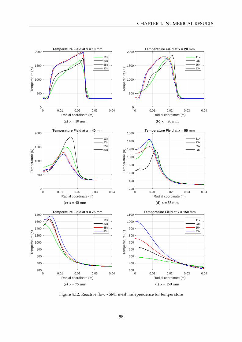
CHAPTER 4. NUMERICAL RESULTS
0 0.01 0.02 0.03 0.04
Radial coordinate (m)
0
500
1000
1500
2000
Tem
pera
ture
(K
)
Temperature Field at x = 10 mm
11k23k55k83k
(a) x = 10 mm
0 0.01 0.02 0.03 0.04
Radial coordinate (m)
0
500
1000
1500
2000
Tem
pera
ture
(K
)
Temperature Field at x = 20 mm
11k23k55k83k
(b) x = 20 mm
0 0.01 0.02 0.03 0.04
Radial coordinate (m)
0
500
1000
1500
2000
Tem
pera
ture
(K
)
Temperature Field at x = 40 mm
11k23k55k83k
(c) x = 40 mm
0 0.01 0.02 0.03 0.04
Radial coordinate (m)
200
400
600
800
1000
1200
1400
1600
Tem
pera
ture
(K
)
Temperature Field at x = 55 mm
11k23k55k83k
(d) x = 55 mm
0 0.01 0.02 0.03 0.04
Radial coordinate (m)
200
400
600
800
1000
1200
1400
1600
1800
Tem
pera
ture
(K
)
Temperature Field at x = 75 mm
11k23k55k83k
(e) x = 75 mm
0 0.01 0.02 0.03 0.04
Radial coordinate (m)
300
400
500
600
700
800
900
1000
1100
Tem
pera
ture
(K
)
Temperature Field at x = 150 mm
11k23k55k83k
(f) x = 150 mm
Figure 4.12: Reactive flow - SM1 mesh independence for temperature
58
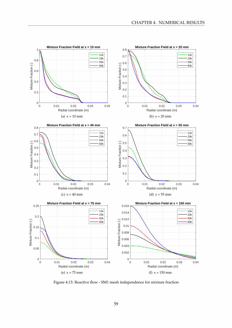
CHAPTER 4. NUMERICAL RESULTS
0 0.01 0.02 0.03 0.04
Radial coordinate (m)
0
0.2
0.4
0.6
0.8
1
Mix
ture
Fra
ctio
n (-
)
Mixture Fraction Field at x = 10 mm
11k23k55k83k
(a) x = 10 mm
0 0.01 0.02 0.03 0.04
Radial coordinate (m)
0
0.1
0.2
0.3
0.4
0.5
0.6
0.7
0.8
Mix
ture
Fra
ctio
n (-
)
Mixture Fraction Field at x = 20 mm
11k23k55k83k
(b) x = 20 mm
0 0.01 0.02 0.03 0.04
Radial coordinate (m)
0
0.1
0.2
0.3
0.4
0.5
0.6
0.7
0.8
Mix
ture
Fra
ctio
n (-
)
Mixture Fraction Field at x = 40 mm
11k23k55k83k
(c) x = 40 mm
0 0.01 0.02 0.03 0.04
Radial coordinate (m)
0
0.1
0.2
0.3
0.4
0.5
0.6
0.7
Mix
ture
Fra
ctio
n (-
)
Mixture Fraction Field at x = 55 mm
11k23k55k83k
(d) x = 55 mm
0 0.01 0.02 0.03 0.04
Radial coordinate (m)
0
0.05
0.1
0.15
0.2
0.25
Mix
ture
Fra
ctio
n (-
)
Mixture Fraction Field at x = 75 mm
11k23k55k83k
(e) x = 75 mm
0 0.01 0.02 0.03 0.04
Radial coordinate (m)
0
0.002
0.004
0.006
0.008
0.01
0.012
0.014
0.016
Mix
ture
Fra
ctio
n (-
)
Mixture Fraction Field at x = 150 mm
11k23k55k83k
(f) x = 150 mm
Figure 4.13: Reactive flow - SM1 mesh independence for mixture fraction
59
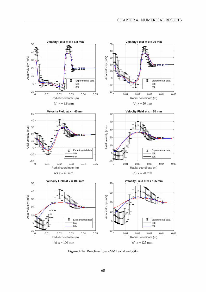
CHAPTER 4. NUMERICAL RESULTS
0 0.01 0.02 0.03 0.04 0.05
Radial coordinate (m)
-10
0
10
20
30
40
50
Axi
al v
eloc
ity (
m/s
)
Velocity Field at x = 6.8 mm
Experimental data55k83k
(a) x = 6.8 mm
0 0.01 0.02 0.03 0.04 0.05
Radial coordinate (m)
-20
-10
0
10
20
30
40
50
Axi
al v
eloc
ity (
m/s
)
Velocity Field at x = 20 mm
Experimental data55k83k
(b) x = 20 mm
0 0.01 0.02 0.03 0.04 0.05
Radial coordinate (m)
-20
-10
0
10
20
30
40
50
Axi
al v
eloc
ity (
m/s
)
Velocity Field at x = 40 mm
Experimental data55k83k
(c) x = 40 mm
0 0.01 0.02 0.03 0.04 0.05
Radial coordinate (m)
-10
0
10
20
30
40
50
Axi
al v
eloc
ity (
m/s
)
Velocity Field at x = 70 mm
Experimental data55k83k
(d) x = 70 mm
0 0.01 0.02 0.03 0.04 0.05
Radial coordinate (m)
-10
0
10
20
30
40
50
Axi
al v
eloc
ity (
m/s
)
Velocity Field at x = 100 mm
Experimental data55k83k
(e) x = 100 mm
0 0.01 0.02 0.03 0.04 0.05
Radial coordinate (m)
-10
0
10
20
30
40
Axi
al v
eloc
ity (
m/s
)
Velocity Field at x = 125 mm
Experimental data55k83k
(f) x = 125 mm
Figure 4.14: Reactive flow - SM1 axial velocity
60
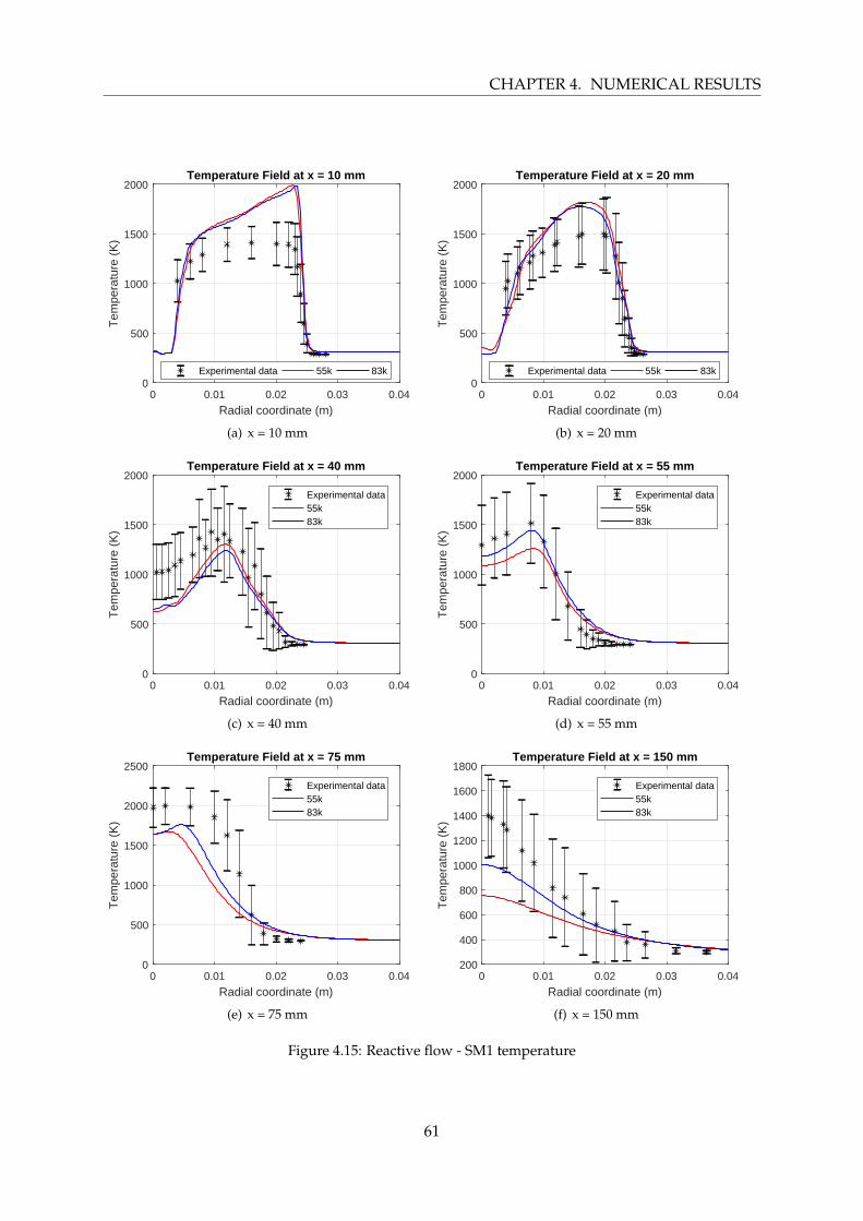
CHAPTER 4. NUMERICAL RESULTS
0 0.01 0.02 0.03 0.04
Radial coordinate (m)
0
500
1000
1500
2000
Tem
pera
ture
(K
)
Temperature Field at x = 10 mm
Experimental data 55k 83k
(a) x = 10 mm
0 0.01 0.02 0.03 0.04
Radial coordinate (m)
0
500
1000
1500
2000
Tem
pera
ture
(K
)
Temperature Field at x = 20 mm
Experimental data 55k 83k
(b) x = 20 mm
0 0.01 0.02 0.03 0.04
Radial coordinate (m)
0
500
1000
1500
2000
Tem
pera
ture
(K
)
Temperature Field at x = 40 mm
Experimental data55k83k
(c) x = 40 mm
0 0.01 0.02 0.03 0.04
Radial coordinate (m)
0
500
1000
1500
2000
Tem
pera
ture
(K
)
Temperature Field at x = 55 mm
Experimental data55k83k
(d) x = 55 mm
0 0.01 0.02 0.03 0.04
Radial coordinate (m)
0
500
1000
1500
2000
2500
Tem
pera
ture
(K
)
Temperature Field at x = 75 mm
Experimental data55k83k
(e) x = 75 mm
0 0.01 0.02 0.03 0.04
Radial coordinate (m)
200
400
600
800
1000
1200
1400
1600
1800
Tem
pera
ture
(K
)
Temperature Field at x = 150 mm
Experimental data55k83k
(f) x = 150 mm
Figure 4.15: Reactive flow - SM1 temperature
61
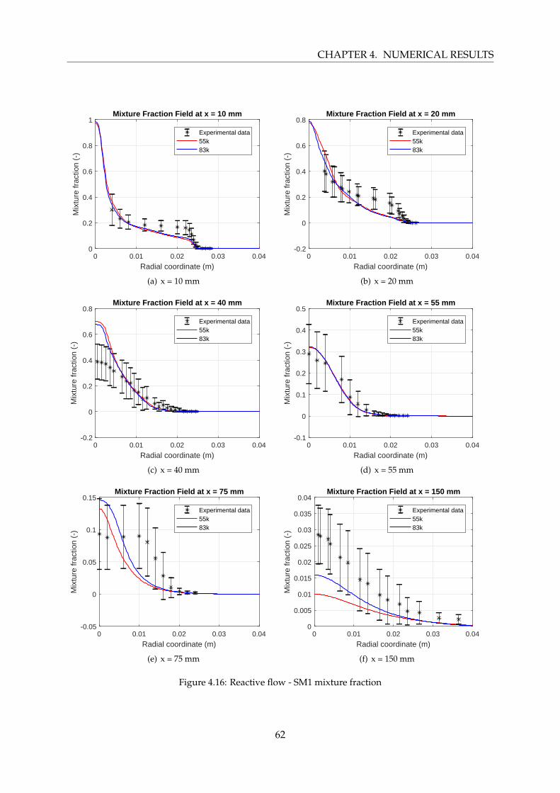
CHAPTER 4. NUMERICAL RESULTS
0 0.01 0.02 0.03 0.04
Radial coordinate (m)
0
0.2
0.4
0.6
0.8
1
Mix
ture
frac
tion
(-)
Mixture Fraction Field at x = 10 mm
Experimental data55k83k
(a) x = 10 mm
0 0.01 0.02 0.03 0.04
Radial coordinate (m)
-0.2
0
0.2
0.4
0.6
0.8
Mix
ture
frac
tion
(-)
Mixture Fraction Field at x = 20 mm
Experimental data55k83k
(b) x = 20 mm
0 0.01 0.02 0.03 0.04
Radial coordinate (m)
-0.2
0
0.2
0.4
0.6
0.8
Mix
ture
frac
tion
(-)
Mixture Fraction Field at x = 40 mm
Experimental data55k83k
(c) x = 40 mm
0 0.01 0.02 0.03 0.04
Radial coordinate (m)
-0.1
0
0.1
0.2
0.3
0.4
0.5
Mix
ture
frac
tion
(-)
Mixture Fraction Field at x = 55 mm
Experimental data55k83k
(d) x = 55 mm
0 0.01 0.02 0.03 0.04
Radial coordinate (m)
-0.05
0
0.05
0.1
0.15
Mix
ture
frac
tion
(-)
Mixture Fraction Field at x = 75 mm
Experimental data55k83k
(e) x = 75 mm
0 0.01 0.02 0.03 0.04
Radial coordinate (m)
0
0.005
0.01
0.015
0.02
0.025
0.03
0.035
0.04
Mix
ture
frac
tion
(-)
Mixture Fraction Field at x = 150 mm
Experimental data55k83k
(f) x = 150 mm
Figure 4.16: Reactive flow - SM1 mixture fraction
62
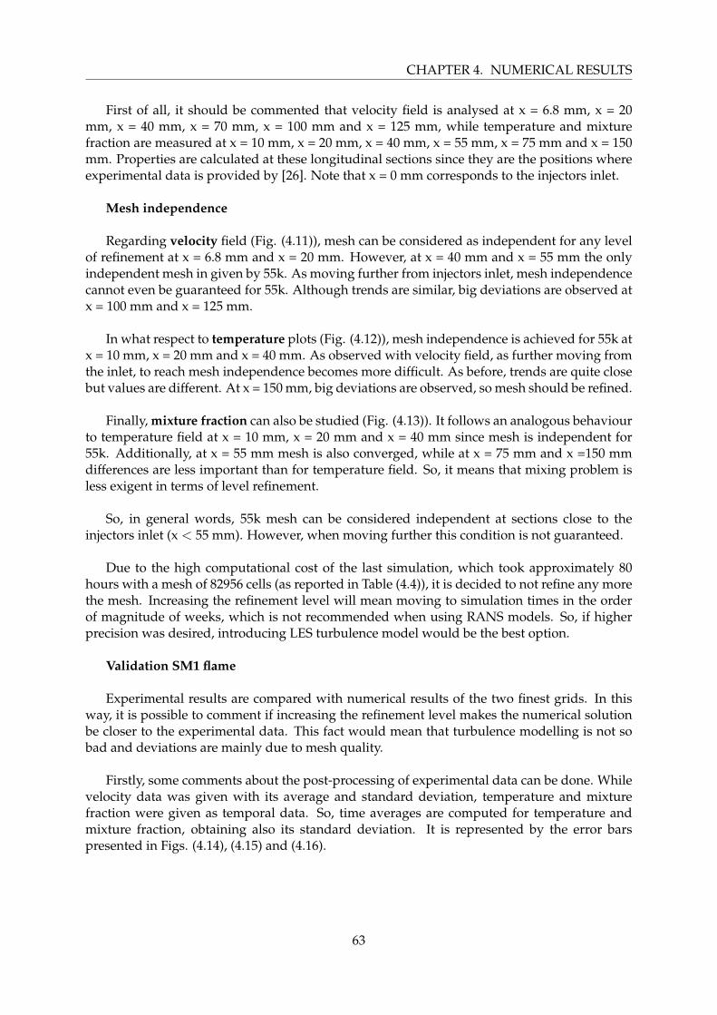
CHAPTER 4. NUMERICAL RESULTS
First of all, it should be commented that velocity field is analysed at x = 6.8 mm, x = 20mm, x = 40 mm, x = 70 mm, x = 100 mm and x = 125 mm, while temperature and mixturefraction are measured at x = 10 mm, x = 20 mm, x = 40 mm, x = 55 mm, x = 75 mm and x = 150mm. Properties are calculated at these longitudinal sections since they are the positions whereexperimental data is provided by [26]. Note that x = 0 mm corresponds to the injectors inlet.
Mesh independence
Regarding velocity field (Fig. (4.11)), mesh can be considered as independent for any levelof refinement at x = 6.8 mm and x = 20 mm. However, at x = 40 mm and x = 55 mm the onlyindependent mesh in given by 55k. As moving further from injectors inlet, mesh independencecannot even be guaranteed for 55k. Although trends are similar, big deviations are observed atx = 100 mm and x = 125 mm.
In what respect to temperature plots (Fig. (4.12)), mesh independence is achieved for 55k atx = 10 mm, x = 20 mm and x = 40 mm. As observed with velocity field, as further moving fromthe inlet, to reach mesh independence becomes more difficult. As before, trends are quite closebut values are different. At x = 150 mm, big deviations are observed, so mesh should be refined.
Finally, mixture fraction can also be studied (Fig. (4.13)). It follows an analogous behaviourto temperature field at x = 10 mm, x = 20 mm and x = 40 mm since mesh is independent for55k. Additionally, at x = 55 mm mesh is also converged, while at x = 75 mm and x =150 mmdifferences are less important than for temperature field. So, it means that mixing problem isless exigent in terms of level refinement.
So, in general words, 55k mesh can be considered independent at sections close to theinjectors inlet (x < 55 mm). However, when moving further this condition is not guaranteed.
Due to the high computational cost of the last simulation, which took approximately 80hours with a mesh of 82956 cells (as reported in Table (4.4)), it is decided to not refine any morethe mesh. Increasing the refinement level will mean moving to simulation times in the orderof magnitude of weeks, which is not recommended when using RANS models. So, if higherprecision was desired, introducing LES turbulence model would be the best option.
Validation SM1 flame
Experimental results are compared with numerical results of the two finest grids. In thisway, it is possible to comment if increasing the refinement level makes the numerical solutionbe closer to the experimental data. This fact would mean that turbulence modelling is not sobad and deviations are mainly due to mesh quality.
Firstly, some comments about the post-processing of experimental data can be done. Whilevelocity data was given with its average and standard deviation, temperature and mixturefraction were given as temporal data. So, time averages are computed for temperature andmixture fraction, obtaining also its standard deviation. It is represented by the error barspresented in Figs. (4.14), (4.15) and (4.16).
63
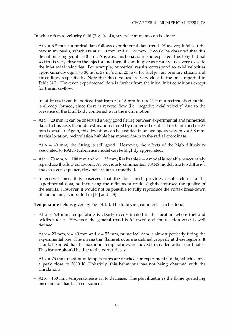
CHAPTER 4. NUMERICAL RESULTS
In what refers to velocity field (Fig. (4.14)), several comments can be done:
− At x = 6.8 mm, numerical data follows experimental data trend. However, it fails at themaximum peaks, which are at r = 0 mm and r = 27 mm. It could be observed that thisdeviation is bigger at r = 0 mm. Anyway, this behaviour is unexpected: this longitudinalsection is very close to the injector and then, it should give as result values very close tothe inlet axial velocities. For example, numerical results correspond to axial velocitiesapproximately equal to 30 m/s, 38 m/s and 20 m/s for fuel jet, air primary stream andair co-flow, respectively. Note that these values are very close to the ones reported inTable (4.2). However, experimental data is further from the initial inlet conditions exceptfor the air co-flow.
In addition, it can be noticed that from r ≈ 15 mm to r ≈ 23 mm a recirculation bubbleis already formed, since there is reverse flow (i.e. negative axial velocity) due to thepresence of the bluff body combined with the swirl motion.
− At x = 20 mm, it can be observed a very good fitting between experimental and numericaldata. In this case, the underestimation offered by numerical results at r = 0 mm and r = 27mm is smaller. Again, this deviation can be justified in an analogous way to x = 6.8 mm.At this location, recirculation bubble has moved down in the radial coordinate.
− At x = 40 mm, the fitting is still good. However, the effects of the high diffusivityassociated to RANS turbulence model can be slightly appreciated.
− At x = 70 mm, x = 100 mm and x = 125 mm, Realizable k− ε model is not able to accuratelyreproduce the flow behaviour. As previously commented, RANS models are too diffusiveand, as a consequence, flow behaviour is smoothed.
− In general lines, it is observed that the finer mesh provides results closer to theexperimental data, so increasing the refinement could slightly improve the quality ofthe results. However, it would not be possible to fully reproduce the vortex breakdownphenomenon, as reported in [16] and [18].
Temperature field is given by Fig. (4.15). The following comments can be done:
− At x = 6.8 mm, temperature is clearly overestimated in the location where fuel andoxidizer react. However, the general trend is followed and the reaction zone is welldefined.
− At x = 20 mm, x = 40 mm and x = 55 mm, numerical data is almost perfectly fitting theexperimental one. This means that flame structure is defined properly at these regions. Itshould be noted that the maximum temperatures are moved to smaller radial coordinates.This feature should be due to the vortex decay.
− At x = 75 mm, maximum temperatures are reached for experimental data, which showsa peak close to 2000 K. Unluckily, this behaviour has not being obtained with thesimulations.
− At x = 150 mm, temperatures start to decrease. This plot illustrates the flame quenchingonce the fuel has been consumed.
64

CHAPTER 4. NUMERICAL RESULTS
− As happened with velocity field, the finest mesh offers more accurate results. In this case,83k mesh is clearly outperforming at x = 55 mm and x = 150 mm. In this last case, it seemsthat even a finer mesh would be able to fully reproduce the experimental temperaturefield.
In what refers to mixture fraction, the following aspects can be pointed out:
− At x = 6.8 mm, the initial conditions can be observed. At r = 0 mm, mixture fractionis almost equal to 1 due to the presence of a fuel predominant mixture. As movingaway from the fuel jet (z = 1), the mixture fraction is reduced due to its mixing withthe oxidizer (z = 0). Once the position of the air co-flow is reached, mixture fraction is setto 0. Regarding the fitting, numerical results are underestimating the experimental data.This behaviour is also found at x = 20 mm.
− At x = 40 mm and x = 55 mm, very good fittings are found except for small valuesof the radial coordinate at x = 40 mm. Until this point, the 4 sections described areapproximately reproducing the mixing in an adequate way.
− At x = 75 mm and x = 150 mm, bigger deviations are found. Note that at x = 150 mm,mixture fraction is very close to 0. This means that fuel has been almost fully consumed.
− Mixture fraction has been found as the less sensible variable to the level of refinement:important differences are not found until x = 75 mm. As happened with velocity andtemperature fields, it could be stated the finest mesh offers better results. At x = 75 mm, itis not so evidence, but this trend is clearly observed at x = 150 mm, where the finest meshprovides numerical results that are closer to the experimental data.
So, after having analysed the velocity, temperature and mixture fraction fields, it can beconcluded that vortex decay structures have not been fully described. While, in general terms,flow behaviour is perfectly captured for the zones close to the injector, results are not sosatisfactory when moving further, i.e. at vortex breakdown and precessing vortex core.
Despite this fact, the mean features regarding swirling flames have been captured:numerical results show a similar trend to experimental data. So, swirl boundary condition hasbeen definitely validated.
To conclude this analysis, temperature field can also be compared with respect tothe temperature field captured experimentally, reported at [32]. Fig. (4.17) contains thisinformation with numerical data taken from 83k mesh. Note that the scale is expressed inK. It can allows observing the main points described previously: temperature field zone iswell described for values of the longitudinal coordinate close to the injectors inlet althoughtheir values are different. Note that experimental temperatures are lower than those obtainednumerically.
As moving far away from the inlet, it can be noticed that the numerical results are toodiffusive compared with experimental data. It can be seen that flame width is clearly smallerand colder (lower temperature).
Analogously, mixture fraction contour plot is reported in Fig. (4.18). In this case, the widthis equal to r = 0.075 m, while the length shown is x = 0.25 m.
65
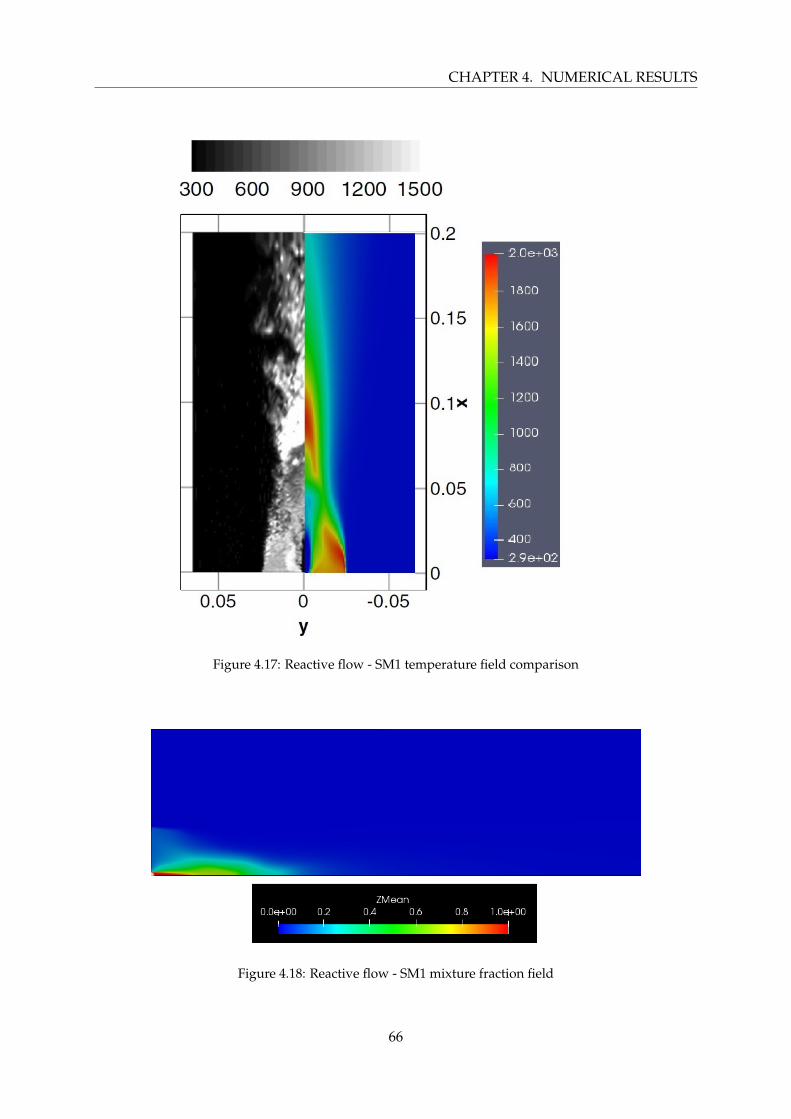
CHAPTER 4. NUMERICAL RESULTS
Figure 4.17: Reactive flow - SM1 temperature field comparison
Figure 4.18: Reactive flow - SM1 mixture fraction field
66
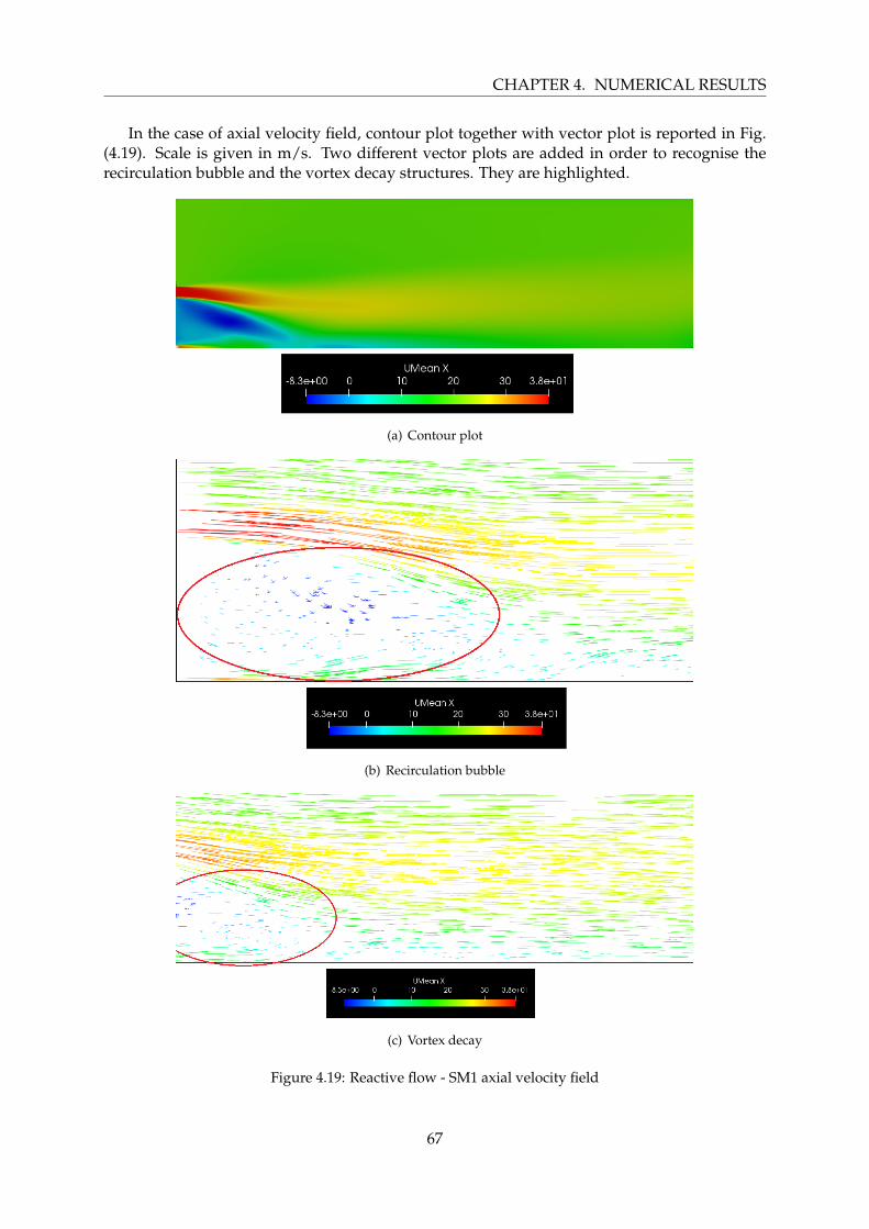
CHAPTER 4. NUMERICAL RESULTS
In the case of axial velocity field, contour plot together with vector plot is reported in Fig.(4.19). Scale is given in m/s. Two different vector plots are added in order to recognise therecirculation bubble and the vortex decay structures. They are highlighted.
(a) Contour plot
(b) Recirculation bubble
(c) Vortex decay
Figure 4.19: Reactive flow - SM1 axial velocity field
67

CHAPTER 4. NUMERICAL RESULTS
68
Chapter 5
Conclusions
Swirling flames constitute a growing point of interest for the combustion field, and itsstudy is what has motivated this thesis project. They offer three main advantages: flamestabilization, reduction of unburned gases and mixing enhancement. These features are due tothe creation of a recirculation zone, which is related to a complex flow structure derived fromthe swirl motion.
To capture this flow phenomenon a suitable turbulence modelling should be chosen. Thisfact raises a detailed discussion in which a compromise between computational cost andaccuracy is found by choosing Realizable k− ε as turbulence model (RANS).
Another main point to consider is the strategy followed to solve the combustion. Themethodology used is based on Computational Fluid Dynamics techniques which allow solvingturbulent combustion problems through the implementation of a numerical approach knownas Flamelet approach. It consists on decoupling the combustion process into two subsets:mixing and flame structure. This method is attainable thanks to the introduction of a passivescalar: the mixture fraction z.
Once the theoretical framework required to solve turbulent non-premixed flames is set, itis time to implement a swirling flow in OpenFOAM. This constitutes the main objective ofthis thesis work. To achieve it, a new boundary condition is set, named swirl. A piece of codeis added for the velocity inlet condition, whose authority is unknown and, then, a validationprocess is carried out. Both non-reactive and reactive flow simulations are performed, whoseanalysis is done by comparing them with experimental data.
Non-reactive flow simulations offer very good results with Realizable k − ε model.However, the flow complexity added when carrying out a simulation regarding SM1 swirlingturbulent non-premixed flame of Sydney’s burner produces a change of scenario: Realizablek − ε model does not provide so accurate results, as well as computational cost is drasticallyincreased. In fact, mesh independence was not achieved since increasing the level refinementwould have mean carrying out computations with time simulations in the order of weeks. Thisis completely inefficient when using RANS turbulence models, since it is a huge computationalcost for the lowest level of turbulence modelling. Once simulations take about a week,introducing LES turbulence model should be considered.
69
CHAPTER 5. CONCLUSIONS
After deeply analysing the results obtained for SM1 flame, it is concluded that furtherrefining the mesh leads to more precise results. However, this numerical results would neverperfectly fit the experimental data due to the limitations given by RANS model, which is notable to perfectly capture the flow behaviour derived from the swirl decay.
Despite this fact, swirl boundary condition is considered to be validated. This fact opensnew possibilities of research.
70
Chapter 6
Prospective research
This thesis project constitutes a starting point for the study of swirling flames inOpenFOAM environment. So, further research could be done in this field thanks to thevalidation process accomplished during this thesis project.
Some topics that could be investigated are proposed, such as:
− LES simulations for swirling non-premixed flames. In this way, turbulence will be solvedat grid level. This fact will allow capturing vortex breakdown and precessing vortex corephenomena accurately.
− LES simulations for designing high pressure combustion chambers with swirl injector.Since LES turbulence models offer a precise description of the swirl decay, LESsimulations can be run to predict combustion chamber performance at a given conditions.In this sense, parametric analysis could eventually be carried out.
71

CHAPTER 6. PROSPECTIVE RESEARCH
72
Chapter 7
Bibliography
[1] Creta, F. Combustion course. Lecture notes - The main definitions of Combustion. Roma.
[2] Creta, F. Conbustion course. Lecture notes - Rankine Hugoniot Part A. Roma.
[3] Poinsot, T., & Veynante, D. (2012). Theoretical and numerical combustion. Toulouse. Cedex:The authors.
[4] Muller, H., Niedermeier, C., Pfitzner, M., & Hickel, S. (2019). Steady LaminarFlamelet Modeling for turbulent non-premixed Combustion in LES and RANS Simulations.Munchen. Retrieved from https://www.sfbtr40.de/fileadmin/Annual-Reports/
annualreport2013/c1-2013.pdf
[5] Caputo, M. (2019). A Flamelet Approach for High Pressure Diluted Non-Premixed Flames (LaureaMagistrale in Ingegneria Spaziale e Astronautica). Sapienza Universita di Roma.
[6] Burke–Schumann flame. (2013). Retrieved from https://en.wikipedia.org/wiki/Burke%
E2%80%93Schumann_flame
[7] Martı Gomez-Aldaravı, P. Unidad 4 - Turbulencia. Valencia.
[8] Teorema π de Vaschy-Buckingham. (2019). Retrieved from https://es.wikipedia.org/
wiki/Teorema_%CF%80_de_Vaschy-Buckingham
[9] Martı Gomez-Aldaravı, P. Tema 11 - Ecuaciones del flujo medio. Valencia.
[10] S. Cocic, A., R. Lecic, M., & M. Cantrak, S. (2014). Numerical analysis of axisymmetricturbulent swirling flow in circular pipe. Retrieved from https://www.researchgate.net/
publication/274505291_Numerical_analysis_of_axisymmetric_turbulent_swirling_
flow_in_circular_pipe
[11] Dolz, V., Hoyas, S., Pla, B., & Fajardo, P. (2012). Mecanica de Fluidos. Valencia: EditorialUniversitat Politecnica de Valencia.
[12] Unknown. Swirling flows. Retrieved from http://www.dartmouth.edu/~cushman/
courses/engs250/Swirling-flows.pdf
[13] Vortex. (2019). Retrieved from https://en.wikipedia.org/wiki/Vortex
[14] H. A. Vaidya et al. (2011). Numerical simulations of swirling pipe flows- decay of swirl andoccurrence of vortex structures. J. Phys.: Conf. Ser. 318 062022. Retrieved from https:
//iopscience.iop.org/article/10.1088/1742-6596/318/6/062022
73
CHAPTER 7. BIBLIOGRAPHY
[15] Valorani, M. Corso di Motori Aeronautici. Appunti - Gas Turbines Combustion Chamber. Roma.
[16] Huang, Y., & Yang, V. (2009). Dynamics and stability of lean-premixed swirl-stabilizedcombustion. Retrieved from https://www.sciencedirect.com/science/article/pii/
S0360128509000094
[17] Stein, O., & Kempf, A. (2006). LES of the Sydney swirl flame series: A study of vortex breakdownin isothermal and reacting flows. Retrieved from https://www.sciencedirect.com/science/
article/pii/S1540748906002598
[18] Yang, Y., & Kaer, S.K. (2012). Comparison of Reynolds Averaged Navier-Stokes Based Simulationand Large-eddy Simulation for One Isothermal Swirling Flow. Retrieved from https://link.
springer.com/article/10.1007/s11630-012-0530-9
[19] Martı Gomez-Aldaravı, P. Tema 6 - Introduccion al CFD. Valencia.
[20] Cuoci, A., Frassoldati, A., Faravelli, T., Ranzi, E., OpenSMOKE++. An object-orientedframework for the numerical modeling of reactive systems with detailed kinetic mechanisms (2015)Computer Physics Communications, 192, pp. 237-264 DOI: 10.1016/j.cpc.2015.02.014
[21] OpenFOAM v6 User Guide: 2 OpenFOAM Tutorials. (2019). Retrieved from https://
cfd.direct/openfoam/user-guide/v6-tutorials/
[22] Swirled inlet – CFD Online Discussion Forums. (2015). Retrieved from https://www.
cfd-online.com/Forums/openfoam-solving/162659-swirled-inlet.html
[23] RNG k-epsilon model – CFD-Wiki, the free CFD reference. Retrieved from https://www.
cfd-online.com/Wiki/RNG_k-epsilon_model
[24] K-epsilon turbulence model. Retrieved from https://en.wikipedia.org/wiki/
K-epsilon_turbulence_model
[25] FLUENT 6.3 User’s Guide - 9.5.3 Turbulence Modeling in Swirling Flows. Retrieved fromhttps://www.sharcnet.ca/Software/Fluent6/html/ug/node397.htm
[26] Aerospace Mechanical and Mechatronic Engineering - The University of Sydney.Retrieved from http://web.aeromech.usyd.edu.au/thermofluids/swirl.php
[27] Turbulence intensity – CFD-Wiki, the free CFD reference. Retrieved from https://www.
cfd-online.com/Wiki/Turbulence_intensity
[28] Martı Gomez-Aldaravı, P. Tema 7 - Preproceso en CFD. Valencia.
[29] Kempf, A., Malalasekera, W., Ranga-Dinesh, K., & Stein, O. (2007). Large Eddy Simulationsof Swirling Non-premixed Flames With Flamelet Models: A Comparison of Numerical Methods.Retrieved from https://link.springer.com/article/10.1007/s10494-008-9147-1
[30] KALT, P., AL-ABDELI, Y., MASRI, A., & BARLOW, R. (2002). Swirling turbulentnon-premixed flames of methane: Flow field and compositional structure. Retrieved from https:
//www.sciencedirect.com/science/article/pii/S1540748902802322
[31] Wolfram—Alpha: Making the world’s knowledge computable. Retrieved from https:
//www.wolframalpha.com/
[32] James, S., Zhu, J., & Anand, M. (2007). Large eddy simulations of turbulent flames using thefiltered density function model. Retrieved from https://www.sciencedirect.com/science/
article/pii/S1540748906001684
74