Accepted Manuscript

LES and DES of Strongly Swirling Turbulent Flow through a Suddenly Ex-

panding Circular Pipe

Ardalan Javadi, Håkan Nilsson

PII: S0045-7930(14)00444-7

DOI: http://dx.doi.org/10.1016/j.compfluid.2014.11.014

Reference: CAF 2735

To appear in: Computers & Fluids

Received Date: 14 June 2014

Revised Date: 14 October 2014

Accepted Date: 7 November 2014

Please cite this article as: Javadi, A., Nilsson, H., LES and DES of Strongly Swirling Turbulent Flow through a

Suddenly Expanding Circular Pipe, Computers & Fluids (2014), doi: http://dx.doi.org/10.1016/j.compfluid.

2014.11.014

This is a PDF file of an unedited manuscript that has been accepted for publication. As a service to our customers

we are providing this early version of the manuscript. The manuscript will undergo copyediting, typesetting, and

review of the resulting proof before it is published in its final form. Please note that during the production process

errors may be discovered which could affect the content, and all legal disclaimers that apply to the journal pertain.

LES and DES of Strongly Swirling Turbulent Flow through a

Suddenly Expanding Circular Pipe

Ardalan Javadi, Håkan Nilsson

Department of Applied Mechanics, Chalmers University of Technology, Gothenburg, SE-

412 96, Sweden

Corresponding author. Tel.:+46(31)772 52 95, Fax: +46(31)18 09 76, Email address:

ardalan.javadi@chalmers.se (Ardalan Javadi).

Abstract

A detailed numerical study is undertaken to investigate the physical processes that are

engendered in the strongly swirling turbulent flows through a suddenly expanding circular pipe.

The delayed DES Spalart-Allmaras (DDES-SA), improved DDES-SA (IDDES-SA), a dynamic

k-equation LES (oneEqLES), dynamic Smagorinsky LES (dynSmagLES) and implicit LES with

van Leer discretization (vanLeerILES) are scrutinized in this study. A comprehensive mesh

study is carried out, and the results are validated with experimental data. The results of different

operating conditions from LES and DES are compared and described qualitatively and

quantitatively. The features of the flows are distinguished mainly on the basis of different levels

of the centrifugal force for different swirls. The numerical results capture the vortex breakdown

with its characteristic helical core, the Taylor-Görtler vortices and the turbulence structures.

Further features are addressed because of the excellent agreement between the numerical and

experimental data. The hybrid behavior of DDES-SA and IDDES-SA is discussed. The results

confirm that LES and DES are capable of capturing the turbulence intensity, the turbulence

production and the anisotropy of the studied flow fields.

Keywords: Swirling Flow, Vortex Breakdown, Sudden expansion, LES, DES

1. Introduction

Confined turbulent swirling flows are encountered in many industrial applications, such as

hydraulic turbines, gas turbine combustors and internal combustion engines. A key feature of the

strongly swirling flows is vortex breakdown. Vortex breakdown is an abrupt change in the core

of a slender vortex and typically develops downstream into a recirculatory “bubble” or a helical

pattern (Leibovich, 1984; Shtern and Hussain, 1999). The vortex breakdown may be beneficial,

e.g. increasing heat transfer or the combustion rate in heat exchangers and combustors, or

detrimental, e.g. yielding pressure pulsations in hydraulic turbines. The characteristics of various

breakdown states (or modes) in swirling flows depend on the swirl number (Sr),

Sr=�

�

� �������

�

� ������

�

, (1)

the Reynolds number (Re),

�� � ��

�, (2)

and geometry-induced axial pressure gradients in the flow. Here R is the radius and r is the radial

position, W and U are the axial and tangential velocities, respectively, Wb is the bulk velocity,

D=50.78×10-3 m is the inlet diameter, ρ is the density, and μ is the dynamic viscosity. Gupta et

al. (1984) observed experimentally that the vortex breakdown for turbulent flows at low swirl

numbers is dominated by large-scale unsteadiness due to the onset of a slowly precessing helical

vortex core. The precessing vortex core is related to the oscillatory motion of non-turbulent

coherent structures, yielding the dominant frequency of the energy spectrum. It is known that, as

the swirl number increases, the oscillatory motion of the coherent structure becomes more

pronounced (Wang et al., 2004). For non-swirl flow, the jet can rotate in either direction, while

Nomenclature

D inlet radios [m]

f frequency [1/s]

k turbulent kinetic average [m2.s-2]

R radius [m]

r, θ radial and tangential position [m]

Re Reynolds number [-]

Sr swirl number [-]

Sr* modified Swirl number [-]

U, W tangential and axial mean velocity [m.s-1]

u'rms, w'rms tangential and axial velocity root

mean square [m.s-1]

Wb inlet bulk velocity [m.s-1]

x, y, z coordination directions [m]

PN, Pshear normal and shear production of

turbulence [m2.s-3]

Puu, Pww tangential and axial components of

production of turbulence [m2.s-3]

Puw shear component production of

turbulence [m2.s-3]

Greek Symbols

δ boundary layer thickness [mm]

δij Kronecker delta [-]

μ dynamic viscosity [kg.s-1.m-1]

ρ density [kg.m-3]

υ kinematic viscosity [m2.s-1]

υt turbulent viscosity [m2.s-1]

when a slight swirl is included, the precessing vortex counter-rotates to the direction of the swirl

(Guo et al., 2002). Several modes of precession are predicted as the swirl intensity increases, in

which the precession, as well as the spiral structure, reverses direction (Zohir et al., 2011). When

the swirl increases to Sr=0.5, a central recirculation zone occurs, which is a typical manifestation

of vortex breakdown (Guo et al., 2002). This central reversed flow is the result of a low-pressure

region created by the centrifugal force. For swirling flow in a straight circular pipe at a fixed Re,

it is well known that, above a threshold swirl number, a disturbance develops along the vortex

core, characterized by the onset of a limited region of reversed flow along the axis. This marks

the transition from a supercritical to a subcritical swirling flow state (Escudier, 1987). As the

swirl number increases to moderate levels, the flow is known to become more axisymmetric with

an on-axis recirculation, marking the onset of bubble-type vortex breakdown.

The first analysis of sudden-expansion pipe flows was made by Borda (1766) and the literature

has since been concerned with confirming his expression for the overall loss. Turbulent swirling

flow through a sudden axisymmetric expansion possesses several distinctly different flow

regimes, such as separation, one or two recirculation regions, high turbulence levels, and

periodic asymmetries under some conditions. The diverging nature of sudden-expansion flow is

known to initiate and lock the location of the precession and flow instabilities. Many researchers

have reported experimental (Wang et al., 2004), flow visualization (Mak and Balabani, 2007),

analytical (Gyllenram et al., 2007) and numerical investigations (Nilsson, 2012) of swirling

flows. However, this flow is still not well understood, especially for strongly swirling flow,

where the swirl number is about unity. There are only a handful of detailed numerical studies

that treat the coherent structures and vortex breakdown (Gyllenram et al., 2006) of the incident

flow. At elevated swirl intensities (Sr ≥ 0.6), the swirling jet emanating from the expansion is

deflected towards the wall, the secondary recirculation region close to the corner contracts and

reversal of the flow becomes evident near the centerline of the expansion (Dellenback et al.,

1988). The global frequency of the flow field belongs to the precessing helical vortex, which

oscillates about the centerline basically in a symmetrical fashion in spite of the instantaneous

asymmetry. The vortex core precession has been experimentally (Dellenback et al., 1988) and

numerically (Guo et al., 2002) observed to be both co-rotating and counter-rotating with the

mean swirl direction. Dellenback et al. (1988) reported that the precessing vortex core vanishes

for Sr~0.4, that there is a bubble-type vortex breakdown for Sr<0.6 and that there is a strong on-

axis tube of recirculating flow for higher swirl numbers. Thus, there is a maximum swirl number

beyond which no precessing vortex core will occur. Dellenback et al. (1988) also reported that

the precession frequencies appear independent at large Reynolds numbers (Re>105) but follow a

slowly decreasing function of Re at lower Reynolds numbers.

Numerical simulation is a very important tool for gaining in-depth knowledge of fundamental

flow physics. Experiments are often limited to a few discrete positions and thereby do not often

provide a complete view of the flow. Numerical results that are validated by experimentally

available data extend the available information and make it possible to draw further conclusions.

Numerical simulation of turbulent swirling flows is however still a challenging tas. Swirling flow

in sudden-expansions has been studied using conventional unsteady Reynolds-averaged Navier–

Stokes (URANS) models (Nilsson, 2012). Such models are primarily useful for capturing large-

scale flow structures, while the details of the small-scale turbulence eddies are filtered out in the

averaging process. In many cases the large-scale structures are also damped by the URANS

modeling, which is formulated to model all the turbulence. The quality of the results is thus very

dependent on the underlying turbulence model. Better approaches should be used to handle the

anisotropic and highly dynamic character of turbulent swirling flows. One approach is the large-

eddy simulation (LES) technique. Only a limited number of LES results of swirling flows are

reported in the literature. Gylleram et al. (2006) used LES to study the swirling flow in the

sudden-expansion of Dellenback et al. (1988), at Re=4.0×104 and Sr=0.6. It was shown that the

frequency of the numerically predicted processing vortex core is not sensitive to the choice of

discretization scheme. Schlüter et al. (2004) performed LES of the swirling flow in a sudden-

expansion studied by Dellenback et al. (1988) for different inlet boundary conditions, and Wang

et al. (2004) performed LES of swirling flows in the sudden expansion-contraction. Most of

these simulations focus on confined flows at moderate Reynolds numbers (Re ~104) and with a

coarse resolution, especially close to the walls. An approach with hybrid URANS-LES is well

suited for such flow configurations. Detached-eddy simulation (DES) is a promising hybrid

URANS-LES strategy capable of simulating internal flows dominated by large-scale detached

eddies at practical Reynolds numbers. The method aims at entrusting the boundary layers with

URANS while the detached eddies in separated regions or outside the boundary layers are

resolved using LES. DES predictions of massively separated flows, for which the technique was

originally designed, are typically superior to those achieved using URANS models, especially in

terms of the three-dimensional and time-dependent features of the flow (Spalart, 2009).

According to Peng (2005), the hybrid techniques can be sub-divided into flow-matching and

turbulence-matching methods. In the flow-matching methods, the spatial location of the interface

between URANS and LES is explicitly defined, and the flow parameters (velocities and

turbulence kinetic energy) are matched at the interface. A serious weakness of this approach is

that it is difficult to define the URANS-LES interface for complicated flow geometries. In the

framework of the turbulence matching method, a universal transport equation is solved in the

entire computational domain. The stress terms in this equation are treated in different ways in the

LES and URANS regions, and the transition between the two modeling approaches is smooth.

There are two recently developed major improvements of DES. The first one, called delayed

DES (DDES), has been proposed to detect the boundary layers and to prolong the URANS

mode, even if the wall-parallel grid spacing would normally activate the DES limiter (Spalart,

2009). The second one, called improved DDES (IDDES), solves the problems with modeled-

stress depletion and log-layer mismatch (Spalart, 2009). Other versions of the turbulence

matching methods using different blending functions to switch the solution between LES and

URANS modes were proposed by Peng (2005), and Davidson and Billson (2006). Nilsson

(2012) evaluated a hybrid turbulence model that was developed by Gyllenram and Nilsson

(2008), limiting the modeled turbulence scales according to the local mesh resolution and CFL

number.

The present work investigates the strongly swirling turbulent flow in the sudden-expansion of

Dellenback et al. (1988). The study scrutinizes the ability of modern highly resolved turbulence

models to capture the rich flow physics. Five operating conditions are investigated, with

Reynolds numbers varying from 3.0×104 to 105, and swirl numbers varying from 0.6 to 1.23.

Such wide range of strong swirl numbers and high Reynolds numbers has received less attention

in the literature. Three LES sub-grid approaches are used: an implicit LES, dynamic

Smagorinsky (Germano et al., 1991) and a dynamic k-equation (Kim and Menon, 1995) model.

Two hybrid RANS-LES models are also evaluated: DDES-SA (based on the Spalart-Allmaras

RANS model, Spalart et al., 2006) and IDDES-SA (Shur et al., 2008). The present work is

original in diverse facets: The turbulent swirling flow in a sudden-expansion is studied using

three highly resolved LES sub-grid approaches. The applicability of hybrid methods for these

flow features is validated by comparing with LES results. An advanced and in-depth exploration

is conducted of hybrid methods in circumstances with a variety of flow dynamics. To investigate

the physical aspects of the flows, the various vortex breakdown states along the axis, and the

associated large-scale instabilities of the flow along the pipe wall, are emphasized. The

turbulence structures and the state of anisotropy of the flow fields are thoroughly discussed to

accentuate the rich unsteady features of strongly swirling flows.

2. Numerical Methods and Turbulence Modeling

The governing equations are the filtered (LES), or ensemble averaged (URANS), continuity and

Navier-Stokes equations for incompressible flow. Applying the filtering operation to the Navier-

Stokes equations yields,

�����

� 0,

������ ���� ����

� � � � 1

���̂�

� ������ �� � �� �

�� . �3�

The last term on the right-hand side includes the turbulent stress due to velocity correlations,

given by:

� � � ����� � ��� ��� . (4)

The closure of the governing equations requires modeling of the turbulent stress tensor. The

equations are discretized using a general finite-volume method with a fully collocated storage,

using the pimpleFoam solver of the OpenFOAM-2.1.x CFD code. The code is parallelized using

domain decomposition and the Message Passing Interface (MPI) library. The simulations are

performed using an AMD Opteron 6220 super computer, using160 cores.

Two convection schemes are studied using a dynamic k-equation LES model, the second-order

central differencing scheme and the second-order van Leer total variation diminishing (TVD)

scheme (van Leer, 1979). The temporal discretization is done using the implicit second-order

backward and Crank-Nicolson schemes. In agreement with Gyllenram et al. (2006), the results

are reasonably independent of the discretization method and therefore the results of the implicit

second-order backward are only shown here. The local turbulence eddy-viscosity is given by

each of the adopted turbulence treatments, listed here.

• The dynamic Smagorinsky LES model (hereafter: dynSmagLES) (Germano et al., 1991).

The dynamic model coefficient, C, is determined as a part of the simulation, based on the

assumption that local equilibrium prevails, i.e. Pksgs-εksgs=0. Negative values of the

effective viscosity are removed by clipping to zero.

• A dynamic k-equation model (hereafter: dynOneEq) (Kim and Menon, 1995). An

important feature of this model is that no assumption is made concerning the local

balance between the subgrid-scale energy production and the dissipation rate is made. A

dynamic localization procedure is used to determine the dissipation and the diffusion

model coefficients.

• An implicit LES method using van Leer damping (van Leer, 1979) (hereafter:

vanLeerILES). The sub-grid scale turbulence is not explicitly modeled but is given by the

numerical diffusion of the convection discretization scheme.

• The hybrid DDES method (Spalart et al., 2006) with Spalart-Allmaras RANS closure

(Spalart and Allmaras, 1994) (hereafter: DDES-SA). This method detects the boundary

layer thickness and prolongs the RANS region compared with the original DES. This

method is less sensitive to wall-parallel grid spacing compared with the original DES,

and, in terms of massive separation, LES mode takes over RANS, which is self-

perpetuating (Spalart et al., 2006).

• The hybrid IDDES method (Shur et al., 2008) with Spalart-Allmaras RANS closure

(Spalart and Allmaras, 1994) (hereafter: IDDES-SA). The DDES functionality of IDDES

becomes active only when the inflow conditions do not have a turbulent content. An

inflow with turbulent content activates wall-modeled LES.

For the presently investigated cases, with high Reynolds numbers and high levels of

anisotropy, turbulence models that do not assume a local balance between the energy production

and the dissipation rate have a much better potential for correctly modeling the sub-grid stresses

(Kim and Menon, 1995). Backscatter of energy from the sub-grid scales to the resolved scales

may occur if the sub-grid scales have energy-containing eddies. Studies show that backscatter

may occur over a significant portion of the cells (Piomelli et al., 1991). Backscatter appears as

negative values of the turbulence production term.

DES is designed to treat the entire boundary layer using a RANS model and to apply an LES

treatment to separated regions. While the original DES method is straightforward and simple in

its definition, it is nevertheless one of the more difficult models to use in complex applications. It

not only requires a fundamental understanding of the model behavior but also a relatively

intricate mesh generation to avoid undefined simulation behavior at the interface between RANS

and LES. An artificial flow separation was reported by Menter and Kuntz (2004) for an airfoil

simulation when the maximum cell edge length (hmax) inside the wall boundary layer was refined

below a critical value of hmax /δ < 0.5-1, where δ is the local boundary layer thickness. This

effect was termed Grid Induced Separation (GIS), as the separation depends on the grid spacing

and not the flow physics. GIS is obviously produced by the effect of a sudden grid refinement

that changes the DES method from RANS to LES, without balancing the reduction in eddy-

viscosity by resolved turbulence contents. Spalart (2009) coined the term Modeled Stress

Depletion (MSD), which refers to the effect of reduction of eddy-viscosity from RANS to LES

without a corresponding balance by a resolved turbulent content. In other words, GIS is a result

of MSD. MSD is essentially a result of insufficient flow instabilities downstream of the switch

from the RANS to the LES model formulation. Spalart et al. (2006) proposed a more generic

formulation of the shielding function, which depends only on the eddy-viscosity and the wall

distance. It can therefore, in principle, be applied to any eddy-viscosity based DES method. The

resulting formulation was termed DDES. The IDDES model features several rather intricate

blending and shielding functions, which allow this model to be used in both DDES and wall-

modeled LES mode (Gritskevich et al., 2012) based on the inflow (or initial) conditions used in

the simulation. The fact that several variants of the DES method, such as DDES and IDDES, are

proposed with rather different characteristics makes the selection of the method and

interpretation of results challenging.

3. Flow Configuration

The case studied in the present work is the swirling flow through a sudden 1:2 axisymmetric

expansion that was experimentally examined by Dellenback et al. (1988). The origin is located

on the centerline at the expansion. The experimental inlet Reynolds number was varied between

3.0×104 and 105, and the swirl number was varied between 0 and 1.2. Measurements of mean and

RMS velocities were made with a laser Doppler anemometer at some cross-sections. For more

details about the validation of the flow in the downstream, see Javadi and Nilsson (2014a). The

present work is devoted to strongly swirling flows, and thus includes only high swirl numbers

(Sr≥0.6). Five highly swirling conditions are thus studied in the present work, see Table 1. The

swirl number is calculated based on the inlet radius and the applied axial and tangential velocity

at inlet boundary condition. Equations (1) and (2) give the details of swirl and Reynolds

numbers, respectively.

Table 1. Studied operation conditions

Reynolds number Swirl number

105 1.23

105 0.74

6.0×104 1.16

3.0×104 0.98

3.0×104 0.6

a)

b) c)

Fig.1. a) experimental cross-sections, (z/D=0.25, 0.5,1 ,2 ,4) b) mesh configuration at expansion,

c) mesh configuration at z/D=1

4. Computational Domain and Mesh Resolution

The experimental study of Dellenback et al. (1988) proved the existence of very large-scale

motions in the form of short regions of outer-layer streamwise fluctuations. Figure 1a shows the

computational domain. The experimental results are available at z/D=0.25, 0.5,1 ,2 ,4. The

computational domain is extended 2D upstream of the expansion and 10D downstream of the

expansion, to reduce the influence of the inlet and the outlet boundary conditions. Gyllenram et

al. (2006), Nilsson (2012) and Javadi and Nilsson (2014a) used the same domain, and the

validation in the downstream raises the least concerns about the viability of the result. Figures 1

b-c show the configuration of the mesh. Table 2 lists the three different mesh resolutions used.

The finest resolution is used only for vanLeerILES. Two different O-grid configurations were

studied to investigate the influence of grid skewness on the first and second invariants, with the

conclusion that the effect is negligible. The maximum aspect ratio of a cell is kept below 200.

The mesh resolutions after the expansion, see Table 2, are comparable with Wu and Moin (2008)

and Jung and Chung (2012), who performed DNS and LES of a turbulent pipe flow, respectively.

Wu and Moin (2008) reported Δz+=8.37 and Δ(Rθ)+=7.01 while Jung and Chung (2012) reported

Δz+=61, Δ(Rθ)+= 23.95 and ymax+=12.2. The mesh resolution units are defined as

Δz+=���

��

�

� Δz, Δ(rθ)+=� ��

�����

�

� Δ (rθ) (5)

where υ is the kinematic viscosity and θ is the tangential position. The y+ is defined as

y+=u*y/υ , u*=(τw/ρ)1/2 , τw=μ(∂u/∂y) (6)

where u* is the friction velocity and τw is the wall friction stress.

The present case is a sudden-expansion with a free-stream shear layer. Therefore the

maximum value of Δ(rθ)+ does not necessarily occur at the wall. Due to the flow configuration,

the maximum y+ value occurs in the moving reattachment point. The maximum CFL number in

average 0.03, with a local maximum of 2. The time steps used for the different mesh resolutions

are given in Table 2.

Table 2 Mesh resolutions and near-wall metrics for the case with Re=105, Sr=1.23

No. Cell

(M)

No. Cells before

expansion*

No. Cells after

expansion*

ymax+, ymin

+ Δzz/D<1+, Δzmax

+ Δ(rθ)max+ core Δt (sec)

8 15,000×90 26,650×248 8, 0.12 15, 20 15 96 10-5

10.4 15,000×150 26,650×306 6, 0.08 13, 15 15 128 7×10-6

12.6 18,500×150 32,000×306 20, 0.06 15, 20 27 160 10-6

*The given number is Ncross-section× Nz

5. Boundary Conditions

The inlet boundary condition for the mean velocity is constructed by spline curves based on the

data measured at z/D=-2. A boundary layer based on the log-law is added between the radially

outermost measuring point and the wall, as suggested by Gyllenram et al. (2006) and used by

Javadi and Nilsson (2014a). Earlier investigations of the same case by Schlüter et al. (2004)

showed that the turbulence level of the inlet boundary condition has strong effects on the mean

velocity profiles if the swirl level is low. However, in the present study, the swirl level is high

enough for high turbulence production and a fast transition to turbulent flow. The results for the

flows under consideration were thus found to be quite insensitive to fluctuations at the inlet,

especially for the higher swirl numbers (Schlüter et al., 2004). The no-slip condition is applied

on the walls and the homogenous Neumann for all boundaries of ksgs. A series of outlet boundary

conditions were evaluated, and the combination of inletOutlet for velocity and homogenous

Dirichlet for pressure was finally found to have the least effect on the upstream flow. The

inletOutlet applies a homogenous Neumann condition but with a limitation of the backflow.

6. Results and discussion

All the studied turbulence treatments are scrutinized for a single condition (Re=105, Sr=1.23),

which has the smallest turbulent structures. For brevity only the result of DDES-SA are

presented for the rest of the operating conditions. The flow parameters are normalized with the

inlet diameter, D, and the inlet bulk velocity, Wb, corresponding to different Reynolds numbers.

6.1. Mean velocity

a) b)

Fig. 2. Mean axial (a) and tangential (b) velocity distributions at cross-section z/D=0.25 for the

case with Re=105, Sr=1.23. The same legend applies for both figures.

-0.4

-0.2

0

0.2

0.4

0.6

0.8

1

1.2

1.4

0 0.2 0.4 0.6 0.8 1

W/W

b

r/D

Measured8M-DDES-SA

dynOneEqdynSmagLES

10M-DDES-SA10M-IDDES-SA

vanLeerILES

-0.4

-0.2

0

0.2

0.4

0.6

0.8

1

1.2

1.4

0 0.2 0.4 0.6 0.8 1

U/W

b

r/D

a) b)

c) d) e)

Fig. 3. Mean axial (W) and tangential (U) velocity distributions at cross-section z/D=0.25 for

DDES-SA a) Re=105, Sr=1.23, b) Re=105, Sr=0.74, c) Re=6.0×104, Sr=1.16, d) Re=3.0×104,

Sr=0.98, e) Re=3.0×104, Sr=0.6.

Figure 2 validates the mean axial and the tangential velocity distributions of different

turbulence treatments for the case with Re=105, Sr=1.23. For brevity, only the results at cross-

section z/D=0.25 are presented here, while the downstream flow is discussed qualitatively.

Javadi and Nilsson (2014a) compared and discussed results at the downstream cross-sections.

The averaging is conducted for at least 50 vortex core precession periods. To avoid redundancy,

only the flow features that are not discussed in the literature are clarified. All the numerical

simulations are capable of capturing the main flow features with acceptable accuracy. For the

axial velocity, almost all turbulence treatments predict a similar qualitative behavior of the on-

axis recirculation region (r/D<0.5). In the outer region, vanLeerILES predicts a slightly different

-0.4

-0.2

0

0.2

0.4

0.6

0.8

1

1.2

1.4

0 0.2 0.4 0.6 0.8 1

(U,W

)/W

b

r/D

Measured WMeasured U

DDES-SA WDDES-SA U

-0.4

-0.2

0

0.2

0.4

0.6

0.8

1

1.2

1.4

0 0.2 0.4 0.6 0.8 1

(U,W

)/W

b

r/D

Measured WMeasured U

DDES-SA WDDES-SA U

-0.4

-0.2

0

0.2

0.4

0.6

0.8

1

1.2

1.4

0 0.2 0.4 0.6 0.8 1

(U,W

)/W

b

r/D

Measured WMeasured U

DDES-SA WDDES-SA U

-0.4

-0.2

0

0.2

0.4

0.6

0.8

1

1.2

1.4

0 0.2 0.4 0.6 0.8 1

(U,W

)/W

b

r/D

Measured WMeasured U

DDES-SA WDDES-SA U

-0.4

-0.2

0

0.2

0.4

0.6

0.8

1

1.2

1.4

0 0.2 0.4 0.6 0.8 1

(U,W

)/W

b

r/D

Measured WMeasured U

DDES-SA WDDES-SA U

behavior than the other turbulence treatments. The DDES-SA (and IDDES-SA) using eight

million cells underestimates the on-axis recirculation, while the corresponding simulations using

10.4 million cells perform qualitatively well. The difference between these two mesh resolutions

is the streamwise (wall-parallel) number of cells. Furthermore, to keep the same maximum

aspect ratio of a cell (~200), the wall-normal spacing is decreased. According to its definition,

the DDES functionality of IDDES should become active only when the inflow conditions do not

have a turbulent content (Shur et al., 2008), while the investigation shows that the IDDES-SA

results differ from those of DDES-SA. This can be related to a high level of recirculation and

production of turbulence in the flow field, which activates the wall-modeled LES mode. It is

worth mentioning that dynOneEq and dynSmagLES predict the flow features reasonably well

using eight million cells and give the same results as with 10.4 million cells.

Figure 3 shows the mean axial and tangential velocity distribution at z/D=0.25 for DDES-SA

for all operating conditions. For all cases, the peak of the axial velocity is at r/D=0.5 and

z/D=0.25, which is right downstream of the edge of the expansion, and the magnitude is

W/Wb~1.3. Comparing Sr=1.23 with 0.74, a higher swirl with the same Re leads to a stronger

backflow on the centerline, i.e. if the swirl intensifies the backflow moves upstream. Dinesh et

al. (2010) also confirm that the vortex breakdown bubble shifts towards the inlet plane with

increased swirl number. Generally, the rate of entrainment of the ensuing jet increases with the

swirl, which gives rise to centrifugal forces and a decrease of the reattachment length. As the

swirl increases from zero to its maximum value, the flow reattachment point moves upstream

from 9 to 2 step heights. The reattachment length is an important parameter in sudden-expansion

flows as it defines the extent of the recirculation and depends on a number of parameters such as

the Re number, the expansion ratio, the free stream turbulence initial and downstream conditions

(Dellenback et al.,1988). A comparison of Sr=1.23 with 0.74 and Sr=0.98 with 0.6 shows that,

as the swirl increases, the recirculation region has a steeper bubble shape. The downstream flow

reveals an on-axis recirculation region that grows longer as the swirl number is reduced. It

reaches about z/D=2.0 for Sr=0.74 and about z/D=1.5 for Sr=1.23. There is a similar trend for

Sr=0.98 and Sr=0.6. Furthermore, since the recirculation region is wider at higher swirl numbers,

it has a steeper cone shape. An interesting observation is that the velocity profiles of Sr=1.23 and

Sr=1.16 are very similar, i.e., for swirl numbers greater than unity, the mean velocity profiles are

even less dependent on the Reynolds number. The on-axis recirculation flow, which onsets the

bubble-type vortex breakdown, increases with the Reynolds number, i.e. the case with Sr=1.23

has a wider bubble than the cases with Sr=1.16 and 0.98. The axial velocity downstream of the

bubble increases to the end of the domain as the axial velocity profile is flattening out.

Furthermore, the static pressure drops at the expansion, and the drop grows as the Reynolds

number increases. The main difference between Sr=0.98 and the profiles of the very similar

conditions of Sr =1.23 and Sr=1.16 is that the axial velocity close to the wall, r/D>0.8, is not as

steep. This can be related to lower amount of mass flux, with respect to the pressure gradient.

Moreover, at the high swirl levels, the flow at the centerline is in the same direction as the mean

flow. The tangential velocity peak at r/D=0.4 is U/Wb~1.2 for three higher swirls.

The most accepted definition of the swirl number is cumbersome insofar as the swirl number

is not known a priori but must be found by integration of the mean velocity profiles according to

eq. (1). Furthermore, Gyllenram et al. (2006) argued that the common definition of the swirl

number is inappropriate for recirculating flow because it results in a lower swirl number for a

given tangential velocity profile, as compared to a non-recirculating flow. Because of the square

in the denominator, only the integrand in the numerator will change sign when backflow occurs.

Thus, Gyllenram et al. (2006) used absolute velocity values in the formulation, hereafter denoted

as Sr*, given by

Sr*=�

�

� ��|��|���

�

� ������

�

. (7)

In cases with an inlet swirl number of about unity, i.e. Sr=1.23, 1.16 and 0.98, the swirl

reduces to Sr~0.4 (Sr*~0.7) directly after the expansion and then increases to Sr~1.5 (Sr*~1.55)

at z/D=1. The swirl number continues to increase to Sr=Sr*~2.1 at z/D=3, and then decreases

further downstream. Generally, this behavior can be related to the bubble type vortex breakdown

that occupies a remarkable part of the cross-section. Due to the vortex breakdown, the axial and

the tangential velocity vanish and appear in the radially same points, see Fig. 3, which leads to a

higher swirl number. The difference between Sr* and Sr in z/D<1 in the recirculation region is

remarkable. For this reason, in term of the features of the flow with a swirl number without the

absolute value in the numerator, the current definition should be treated with caution.

a) b)

Fig. 4. Axial and tangential velocity root mean square distributions at cross-section z/D=0.25 for

the case with Re=105, Sr=1.23.

0

0.2

0.4

0.6

0.8

1

0 0.2 0.4 0.6 0.8 1

Wrm

s/W

b

r/D

MeasureddynOneEqDDES-SA

IDDES-SAvanLeerILES

0

0.2

0.4

0.6

0.8

1

0 0.2 0.4 0.6 0.8 1

Urm

s/W

b

r/D

MeasureddynOneEqDDES-SA

IDDES-SAvanLeerILES

a) b)

c) d) e)

Fig. 5. Axial and tangential velocity root mean square distributions at cross-section z/D=0.25 for

cases a) Re=105, Sr=1.23, b) Re=105, Sr=0.74, c) Re=6.0×104, Sr=1.16, d) Re=3.0×104, Sr=0.98,

e) Re=3.0×104, Sr=0.6.

6.2. Turbulence intensity

Figures 4 and 5 show the root mean square of the axial, w'rms, and tangential, u'rms, velocity

fluctuations at cross-section z/D=0.25. Javadi and Nilsson (2014a) compared and discussed the

velocity fluctuations at the downstream cross-sections. The dynOneEq treatment predicts a

slightly higher level of turbulence intensity compared to the other treatments. The accuracy of

the vanLeerILES treatment is promising for this kind of flow, even close to the wall where the

mesh resolution should be on the coarse side for an implicit LES. The hybrid methods generally

predict a lower peak compared to LES, which can be related to the switching between RANS and

LES, see Fig. 4 . The double-peaked profiles of u'rms are predicted reasonably well, although the

0

0.2

0.4

0.6

0.8

1

0 0.2 0.4 0.6 0.8 1(U

rms,

Wrm

s)/W

b

r/D

Measured WrmsMeasured Urms

DDES-SA WrmsDDES-SA Urms

0

0.2

0.4

0.6

0.8

1

0 0.2 0.4 0.6 0.8 1

(Urm

s,W

rms)

/Wb

r/D

Measured WrmsMeasured Urms

DDES-SA WrmsDDES-SA Urms

0

0.2

0.4

0.6

0.8

1

0 0.2 0.4 0.6 0.8 1

(Urm

s,W

rms)

/Wb

r/D

Measured WrmsMeasured Urms

DDES-SA WrmsDDES-SA Urms

0

0.2

0.4

0.6

0.8

1

0 0.2 0.4 0.6 0.8 1

(Urm

s,W

rms)

/Wb

r/D

Measured WrmsMeasured Urms

DDES-SA WrmsDDES-SA Urms

0

0.2

0.4

0.6

0.8

1

0 0.2 0.4 0.6 0.8 1

(Urm

s,W

rms)

/Wb

r/D

Measured WrmsMeasured Urms

DDES-SA WrmsDDES-SA Urms

on-axis peak is lower and the off-axis peak, which caused by the shear layer, is higher than what

is suggested by the experiment. The flow presents a double- or triple-peaked in w'rms, see in

particular Fig 5b. The first peak is arises from the same physics as that in confined jet flow. The

second peak is due to the turbulence generated by the separation at the expansion edge, similar to

the flow over a backward facing step. The third peak is the wall-effect. The experiment does not

distinctly capture the second peak, although there is a clear tendency. The velocity fluctuation

levels of the turbulent flow are highest in the core region. These fluctuations are apparently

induced by the high velocity gradients in the core, and the very weak motion of the core

(Derksen, 2005). As the swirl number increases to about unity, the first two peaks merge, see

Fig. 5 for Sr=1.23, 1.16 and 0.98, while the third peak goes closer to the wall and becomes

stronger. As the swirl number decreases, the first peak moves closer to the centerline due to the

narrower on-axis recirculation. It shows that the jet emanates closer to the centerline when the

swirl decreases. The main fluctuations of the tangential velocity component occur along the

centerline and in the shear layer emanating from the edge of the sudden-expansion. It is worth

mentioning that the experiment suggests that the second peak is closer to the main stream, while

it is numerically predicted closer to the wall. Furthermore, the magnitudes of the peak are still

independent of the Reynolds number but intensified with an increased swirl. All simulations

predict the turbulent fluctuations qualitatively well.

Having established good agreement of the numerical results with the experimental

measurements of Dellenback et al. (1988), these can be used to elaborate on the physics of the

flow fields by visualizing the instantaneous coherent structures of the flow. The highly swirling

flow can be categorized as an extremely turbulent flow because of the sudden jump in the

turbulence intensity. In case Sr=1.23, the turbulence intensity ascends to 67% after the

expansion and then descends. Dellenback et al. (1988) reported that the turbulence intensities at

the highest swirl levels were found to reach 60%. The confinement and the separating nature of

the expansion flow are known to intensify the helical precession and the flow instabilities. In

Sr=0.74, the turbulence intensities are augmented to 48% at z/D=0.5 and then reduced. The

turbulent intensity of the flow is, similar to the other quantities, a function of the swirl but less a

function of the Reynolds number. As reported above, the swirl, and consequently the turbulent

intensity still is intensified after the expansion due to the vortex breakdown. The diffusion rates

are elevated with high levels of turbulence kinetic energy, and the thickness of the viscosity-

dominated sublayer is reduced.

6.3. Instantaneous Flow Features

Figure 6 shows the viscosity ratio, υt/υ , of DDES-SA, for the case Sr=1.23 and for two mesh

resolutions. The high ratio region corresponds to where URANS is prominent and the low ratio

region corresponds to where LES is used. The DDES is developed from DES with the purpose of

extending the RANS modeling further away from the viscous sub-layer, while the LES mode

takes over in massive separation regions (Spalart et al., 2006). Javadi and Nilsson (2014b)

studied the hybrid methods in a flow generated by a swirl generator. They showed that the

DDES-SA switches to LES still very close to the wall. However, the results show that this

behavior is followed in neither the coarse nor the fine mesh resolution. Although the results of

the coarse and the fine resolution are different for the case of Sr=1.23, the hybrid methods are

less mesh dependent at other operating conditions. In other word, LES is still more robust than

DES for certain flow conditions. To confirm Spalart et al. (2006), DDES-SA is still sensitive to

the wall-parallel resolution for certain flow conditions, see Table 2 for details on the mesh

resolutions.

Figure 7 shows the streamlines at z/D=0.5 for two cases, Sr=1.23 and Sr=1.16. The flow is

divided to an inner part, which is the swirling jet flow, and an outer part which is the primary

recirculation region caused by the separation from the edge of the expansion. For Sr=1.23, the

on- and off-axis recirculation regions are stronger. There are smaller coherent structures adjacent

to the wall, which these structures are a special kind of streak called Taylor-Görtler vortices

(Escudier et al., 1988). The Taylor-Görtler vortices form on the tube wall, mix up the fluid

outside the core, and result in a relatively uniform stable distribution of vorticity in this outer

region. These streaks are presumably related to the centrifugal force of the flow along the

concave wall boundary layer. The issuing of Taylor–Görtler vortices as also observed by

Escudier (1987) for a related swirling flow experiment in a straight pipe geometry. These

structures are well captured although occurring in the region where RANS modeling is

prominent.

Figure 8 shows the q-criterion for different cases. For a swirl number about unity, the flow

downstream of the expansion is more organized and is characterized by the onset of a large-

scale, full-length, columnar vortex along the pipe centerline, which rotates in the mean flow

swirl direction and becomes intertwined. Salas and Kuruvila (1989) reported that near the inflow

the solutions become independent of Reynolds number. The emergence of the large-scale on-axis

vortex at high swirl numbers is obviously related to the on-axis, elongated pocket of the

recirculating flow on the tube centerline. For high swirl numbers, the on-axis vortical structure

strengthens, Figs. 8a and b, and its bend and the adverse longitudinal pressure gradient are

intensified. Dellenback et al. (1988) reported that, at high Reynolds numbers, the vortex

bre

me

wit

ent

num

coh

dec

flux

a)

b)

eakd

ean

th a

tire

mbe

here

crea

x b

Fig

dow

flo

an in

flo

er.

enc

ase.

eco

g. 6

wn p

w i

ncr

ow i

As

ce st

. Th

ome

. V

pat

is si

reas

is s

me

truc

his

es s

Visco

ttern

imi

sing

ubc

enti

ctur

tren

sma

osit

n is

ilar

g sw

criti

ione

res

nd

aller

ty r

s fea

to

wirl

ical

ed a

clo

is s

r.

ratio

atur

low

l nu

l. T

abo

ose

simi

o o

red

wer

umb

The

ove,

to t

ilar

f D

Sr

d by

Re

ber,

stre

, wh

the

r to

DDE

r=1

y the

eyno

, the

eng

hen

wa

the

ES-S

1.23

e fo

old

e br

gth

n th

all a

e ca

SA

3, a

orm

s nu

reak

of v

he sw

and

ase

A in

a) 8×

mati

um

kdo

vor

wir

d in

wh

the

×10

ion

mber

own

rtice

rl de

the

hen

e ce

06 c

of

rs. I

n re

es i

ecre

e pe

the

ente

cells

a pr

It w

egio

is in

eas

erip

e Re

er p

s b)

rec

was

on m

n di

ses,

pher

eyn

lan

) 10

ess

als

mov

irec

the

ry o

nold

ne a

0.4×

sing

o o

ves

ct re

e ce

of th

ds n

and

×10

g sp

obse

up

elat

entr

he o

num

z/D

06 ce

piral

erve

pstre

tion

rifu

on-

mbe

D=1

ells

l ev

ed b

eam

n bo

gal

-axi

r de

1 fo

s.

ven

by E

m un

oth

l for

is re

ecre

or th

if t

Esc

ntil

to s

rce

ecir

eas

he c

the

cudi

l pr

swi

dec

rcul

es a

case

cor

ier

acti

irl a

cre

lati

and

e w

rres

(19

ical

and

ase

on

d th

ith

spo

987

lly

d Re

es an

zon

e m

Re

ondi

) th

the

eyn

nd

ne

mass

=10

ing

hat,

e

old

the

s

05,

ds

e

a) b)

Fig. 7. Swirling flow visualized by instantaneous streamtraces z/D=0.5 for cases a) Re=105,

Sr=1.23 and b) Re=6.0×104, Sr=1.16.

a) b)

c) d

Fig. 8. Vortex breakdown visualized by instantaneous iso-surface of q-criterion (=10000) for the

case a) Re=105, Sr=1.23, b) Re=6.0×104 Sr=1.16, c) Re=3.0×104, Sr=0.98, d) Re=3.0×104,

Sr=0.6.

6.4. Energy Spectrum

Large-eddy simulation is ordinarily addressed using a spatial filtering but without explicitly

stating the associated time filtering (Pope, 2005). Although there is no reference to determine

what timescales are well resolved numerically and physically, we tried to apply fine time steps to

mask the issue. Figure 9 shows the power spectra density captured at (r/D, z/D)=(0.5, 0.25). The

energy spectrum shows that the dominant frequency depends on the swirl number. The study of

the iso-surface of the pressure in successive timesteps shows that the flow pulsations (lashes)

caused by the on-axis recirculation which occupies a considerable portion of the cross-section,

see Fig. 3. Theses lashes increase at higher Reynolds numbers. The power spectrum at the point

shows that the flow is characterized by the existence of the vortex breakdown with dominant

frequencies of about 0.75, 0.86, 1.47 and 1.71, respectively for Sr=1.23. The dominant frequency

varies with the configuration of the inlet, presumably related to differences in the initial shear-

layer of the jet, often characterized by the boundary-layer displacement thickness. In the

downstream, the flow looks like a well developed turbulent flow, with most of its power in its

harmonics. All the spectral components indicate a strong dissipation and a reduction in the total

turbulent kinetic energy while the rate is higher for larger swirls and is generally like an isotropic

turbulence, see subsection 6.6 for more details. It can be seen that the slope changes similarly

from energetic to inertial range in all cases. Commonly, LES somewhat overestimates the energy

content at large-scales and gives a plateau; however, as the structures break down, the energy

content rapidly loses energy fast and the slope increases. This can be related to the frequency of

the SGS filtering and an attempt is made to mask this by fine resolution (Sagaut, 2002). With

regard to the accuracy, this type of finding should nonetheless be treated with caution because

the conclusions may be reversed if we bring in an additional parameter, which is the numerical

scheme or higher advanced solution, DNS. As the cell size decreases, the diffusion decreases and

the model resolves smaller flow structures. Nonetheless, at this stage, we tried to use a self-

adaptive subgrid models that is able to tune induced dissipation so that the sum of the numerical

and subgrid dissipation will reach the required level to obtain physical results.

a) b)

c) d)

Fig. 9. Power spectra at a selected streamwise location (r/D, z/D)=(0.5,0.25), for the case a)

Re=105, Sr=1.23, b) Re=6.0×104 Sr=1.16, c) Re=3.0×104, Sr=0.98, d) Re=3.0×104, Sr=0.6.

An implicit LES technique is also scrutinized because DNS of the current test case is hard to

afford. Interestingly, the same change of the slope at high frequency is observed in all cases,

which shows the energy transfer from large- to small-scales. This transfer rate of the energy

cascade from the large to small-scale motions is accelerated downstream.

6.5. Turbulence Production

For a three-dimensional incompressible turbulent flow, the production terms in the transport

equations for the Reynolds shear stress and turbulent kinetic energy are given by

-Production=�������/��� � ����/�������

� ���/�� � ����/�������

�������������������������

+� ��/�� � � ��/�� � ����/�������

� ����/�� � ���/�� � ���/�������������������������������������������������������

(8)

where uiuj are the Reynolds stresses and ∂Ui/∂xj are the velocity gradients. All terms normalized

by W3b/D are shown in Fig. 10. Since the distribution of the RMS velocity is reasonable, the

different terms of the turbulent kinetic energy equation should be mimicked fairly plausibly

(Javadi, 2013). Two cases with, Sr=1.23 and 0.74 and the same Reynolds number, are discussed

here to exclude the Reynolds number effects. The normal production terms, Puu and Pww, and the

shear term, Puw , are depicted individually and in total, PN and Pshear , to shed light on the physics

of turbulence in the incident flow. Primarily, the comparable level of the production before and

after the expansion confirms what was said earlier about the independence of the simulation from

the inlet, i.e. the flow features at the separation edge are characterized by the turbulence that is

generated. Secondly, the studied flows before and after the expansion are rather different for

various cases. The level of increase of the production after the expansion for Sr=0.74 is large,

which is the reason for the augmentation of the turbulent intensity in the near downstream after

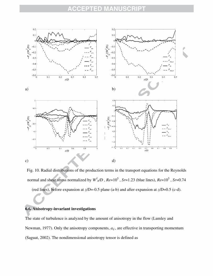
the expansion (z/D<0.5), see section 6.2. Figures10a and b show the production of turbulence

before the expansion. Most of the turbulence is produced by Puu and Pww before the expansion

while Puu is primarily responsible for the backscatter. For Sr=0.74, most of the turbulence is

produced about the axis, while, for Sr=1.23, it is distributed more along the radius. This can be

related to a larger centrifugal force in Sr=1.23. The ∂W/∂z is negative except in the near wall

region where the helical vortex forms a locally high velocity region. This can be the reason for

backscatter.

The dominant shear term is Puw which is distributed more along the radius. The Puw of Sr=1.23

is twice as large as that of Sr=0.74. Regardless of the Reynolds and swirl numbers, the PN is

negligible compared to Pshear, which shows the rich turbulent nature of the flow.

Figures 10c and d show the production after the expansion for the two cases. There is a free

shear layer caused by the separation The shear layer has two edges; the former is a high velocity

edge and the latter is a low velocity edge. These two edges play important roles in the turbulence

nature for strongly swirling flows. The dominant normal terms are still Puu and Pww but hey have

an opposite sign, which naturalizes PN in Sr=0.74. In other words, the amount of the cascade and

the backscatter are the same. In Sr=1.23, Pww is still larger than Puu. Most of the Pww occurs

along the high velocity edge while Puu is on the low velocity edge. This trend is the reverse for

the operation conditions Sr=0.98 and 0.6.

The only shear production term after the expansion is Puw, which is influenced by the free shear

layer of the separation at the edge. The level of Puw compared with normal terms is remarkably

larger. For Sr=1.23, the high velocity edge is larger than the other edge. This is the reverse for

Sr=0.74. The production is almost negligible further downstream (z/D>1). At mid-downstream,

redistribution plays a more important role, and far downstream, dissipation is escalated.

a) b)

c) d)

Fig. 10. Radial distributions of the production terms in the transport equations for the Reynolds

normal and shear stress normalized by W3b/D , Re=105 , Sr=1.23 (blue lines), Re=105 , Sr=0.74

(red lines), before expansion at z/D=-0.5 plane (a-b) and after expansion at z/D=0.5 (c-d).

6.6. Anisotropy-invariant investigations

The state of turbulence is analyzed by the amount of anisotropy in the flow (Lumley and

Newman, 1977). Only the anisotropy components, aij , are effective in transporting momentum

(Saguat, 2002). The nondimensional anisotropy tensor is defined as

ij

ji

ij k

uua δ

3

1

2−= , (9)

with the turbulent kinetic average k and the Kronecker delta δij . The anisotropy of a flow can be

derived from the Reynolds stresses τij=-ρ‹uiuj› by subtracting the isotropic part from τij and

normalizing with τss=-ρ‹usus› . This leads to the nondimensional anisotropy tensor. The

nondimensional anisotropy tensor, aij, is previously defined in (10). Tensor aij has three scalar

invariants

aii=0 , II=aijaji , III=aijajkaki . (10)

By cross-plotting II and III, the state of turbulence in a flow can be analyzed with respect to its

anisotropy. The isotropic turbulence is found at the origin where II = III = 0. Figure 11 shows the

states of turbulence at z/D=0.25 and 0.5, where the most anisotropy may occur. It is found that

large degrees of turbulent anisotropy occur in the region that is dominated by the oscillating

vortex core. Further downstream, the degree of turbulent anisotropy is almost negligible. As

expected, the present swirling jet is highly anisotropic. If the scalar invariants II and III are

evaluated for the case of a two-component turbulence, i.e. one component of the velocity

fluctuations is negligibly small compared with the other two, this leads to II = 2/9 + 2III. Doing

the same for the axisymmetric turbulence, i.e. two components are equal in magnitude, yields II

= 3/2(4/3|III|)2/3. Hence, if these relations are cross-plotted, as done in Fig. 11, they define a

narrow region called the anisotropy-invariant map. All physically realizable turbulence has to lie

within this small region. However, different states of turbulence are represented by different

parts of the map.

The left branch of the map (III < 0) describes axisymmetric turbulence, in which one

component of the velocity fluctuations is smaller than the other two. The simplest example of

this type is the passage of grid turbulence through an axisymmetric contraction, which also

happens in the current flow field. Due to the on-axis recirculation, the streamwise velocity

fluctuation is smaller than the other two on the centerline at z/D=0.25, see also Figs. 4a and b. In

Fig. 11, the points at the centerline and the wall are denoted by ‘C’ and ‘W’, respectively. In

contrast, the axisymmetric turbulence on the right side (III > 0) is characterized by one

fluctuating component that dominates over the other two. This holds for grid turbulence through

an axisymmetric sudden-expansion, which the streamwise velocity fluctuation is considerable in

0.2<r/D<0.6, see Figs. 4a and 11. The third boundary line on the top of the map is the limiting

case of a two-component turbulence, as it can be found in the direct vicinity of walls (Javadi and

El-Askary, 2012). Here, the radial component of the velocity fluctuations tends towards zero,

leaving only the wall-parallel components, while the streamwise velocity fluctuation is larger

than the tangential velocity fluctuation, see Fig. 4. The wall points tend to the right part of the

graph. It must be noted that, taking the entire flow into account, all states indeed lie within the

invariant map, as is required by realizability constraints. The wall end point of the profiles lies at

the two-component limit, and the centerline end point lies at axisymmetric contraction limit for

all cases. The state of turbulence tends quickly to isotropy due to the high level of redistribution

after the expansion.

a) b)

Fig. 11. Anisotropy-invariant mapping in two streamwise planes, for the case with a) Re=105,

Sr=1.23 b) Re=105, Sr=0.74. ‘C’ and ‘W’ denote centerline and wall points of the trace,

respectively.

7. Conclusion

The strongly swirling turbulent flow through an abrupt expansion was explored using LES and

DES. The LES captures main features of the flow in a plausible manner. The applicability of

hybrid RANS-LES methods are also scrutinized, the DDES-SA is capable of capturing the

physics of the flow with reasonable accuracy while still being sensitive to wall-parallel

resolution. To predict a certain flow condition with DDES-SA (Re=105, Sr=1.23) with the same

level of accuracy as LES, a finer resolution is needed. The IDDES-SA behaves as wall-modeled

LES in the flows with a high recirculation level, even though no turbulent content is applied at

the inlet.

The key feature of the high swirl flow is the vortex breakdown and the on-axis recirculation

region. The distribution of the on-axis recirculation region varies with different Re and Sr. The

intertwined nature of the coherent structure due to the vortex breakdown is broader and steeper

for higher Re and Sr. The dominant frequency, the precessing helical vortex, of the flow is

insensitive to Reynolds number for a swirl number of about unity. The level of the turbulence

and the turbulence production increases remarkably with the swirl number, while the state of

isotropy is not susceptible to Re and Sr. The flow is anisotropic immediately after expansion,

while it rapidly becomes isotropic due to the redistribution between velocity fluctuations.

Acknowledgement

The research presented was carried out as a part of the ‘‘Swedish Hydropower Centre –

SVC’’. SVC is established by the Swedish Energy Agency, Elforsk and Svenska Kraftnät

together with Luleå University of Technology, The Royal Institute of Technology, Chalmers

University of Technology and Uppsala University, www.svc.nu.

The computational facilities are provided by C3SE, the center for scientific and technical

computing at Chalmers University of Technology, and SNIC, the Swedish National

Infrastructure for Computing.

References

Borda, J.C., 1766. Memoire sur l'ecoulement des fluides par les orifices des vases. Memoire de

l'academie Royale des Siences.

Davidson, L., Billson, M., 2006. Hybrid LES–RANS using synthesized turbulent fluctuations

for forcing in the interface region. Int. J. Heat Fluid Flow, 27, 1028–1042.

Dellenback, P.A., Metzger, D.E., Neitzel, G.P., 1988. Measurements in turbulent swirling flow

through an abrupt axisymmetric expansion. AIAA J. 26(6), 669–681.

Derksen, J.J., 2005. Simulations of confined turbulent vortex flow. Comput. Fluids, 34 (3)

301–318.

Dinesh, K.K.J., Kirkpatrick, M.P., Jenkins, K.W., 2010. Investigation of the influence of swirl

on a confined co-annular swirl jet. Comput. Fluids, 39(5), 756–767.

Escudier, M., 1987. Confined vortices in flow machinery. Annu. Rev. Fluid Mech. 19, 27–52.

Escudier, M., 1988. Vortex breakdown: Observations and explanations. Prog. in Aerospace

Sci. 25 (2), 189–229.

Germano, M., Piomelli, U., Moin, P., Cabot, W., 1991. A dynamic subgrid-scale eddy

viscosity model. Phys. Fluids, 3 (7), 1760-1765.

Gritskevich, M.S., Garbaruk, A.V., Schütze, J., Menter, F.R., 2012. Development of DDES

and IDDES formulations for the k-ω shear stress transport model. Flow Turbul. Combust. 88,

431–449.

Guo, B., Langrish, T.A.G., Fletcher, D.F, 2002. CFD simulation of precession in sudden pipe

expansion flows with low inlet swirl. Appl. Math. Model. 26(1), 1–15.

Gupta, A.K., Lilley, D.G., Syred, N., 1984. Swirl Flows. Abacus Press, Tunbridge Wells, Kent.

Gyllenram, W., Nilsson, H. Design and validation of a scale-adaptive filtering technique for

LRN turbulence modeling of unsteady flow, J. Fluid Eng.-T ASME, 130(5), 2008.

Gyllenram, W., Nilsson, H., Davidson, L., 2006. Large eddy simulation of turbulent swirling

flow through a sudden expansion. 23rd IAHR Symposium, Yokohama.

Gyllenram, W., Nilsson, H., Davidson, L., 2007. On the failure of the quasi-cylindrical

approximation and the connection to vortex breakdown in turbulent swirling flow. Phys. Fluids,

19, 045108.

Javadi A., 2013. Numerical predictions of slot synthetic jets in quiescent surroundings.

Progress in Computational Fluid Dynamics, Int. J., 13 (2), 65 - 83.

Javadi, A. and Nilsson, H., 2014a. A comparative study of scale-adaptive and large-eddy

simulation of highly swirling turbulent flow through an abrupt expansion, 27th IAHR

Symposium on Hydraulic Machinery and Systems, Montreal, Canada.

Javadi, A. and Nilsson, H., 2014b. LES and DES of swirling flow with rotor-stator

interaction, 5th symposium of hybrid RANS-LES method, Texas A&M university, USA.

Javadi, A., El-Askary, W., 2012. Numerical prediction of turbulent flow structure generated by

a synthetic cross-jet into a turbulent boundary layer. Int. J. Numer. Meth. Fluids, 69 (7), 1219-

1236.

Jung, S.Y., Chung Y.M., 2012. Large-eddy simulation of accelerated turbulent flow in a

circular pipe. Int. J. Heat Fluid Flow, 33, 1–8.

Kim, W.W., Menon, S., 1995. A new dynamic one-equation subgrid-scale model for large

eddy simulations. AIAA Paper, Reno, NV.

Leibovich, S., 1984. Vortex stability and breakdown: survey and extension. AIAA J. 22, 1192–

1206.

Lumley, J.L., Newman, G., 1977. The return to isotropy of homogeneous turbulence. J. Fluid

Mech. 82, 161–178.

Mak, H., Balabani, S., 2007. Near field characteristics of swirling flow past a sudden

expansion. Chem. Eng. Sci . 62, 6726–6746.

Menter, F.R., Kuntz, M., 2002. Adaptation of eddy-viscosity turbulence models to unsteady

separated flow behind vehicles. McCallen, R., Browand, F., Ross, J. (eds.) Symposium on the

aerodynamics of heavy vehicles: trucks, buses and trains. Monterey, USA.

Nilsson, H., 2012. Simulations of the vortex in the Dellenback abrupt expansion, resembling a

hydro turbine draft tube operating at part-load. 26th IAHR Symposium, Beijing.

Peng, S., 2005. Hybrid RANS–LES modeling based on zero- and one-equation models for

turbulent flow simulation. Proceedings of the 4th International Symposium on Turbulence and

Shear Flow Phenomena. 1159–1164.

Piomelli, U., Cabot, W.H., Moin, P., Lee, S.,1991. Subgrid-scale backscatter in turbulent and

transitional flows. Phys Fluids A, 3, 1766-1771.

Pope, S.B., 2005. Turbulent flows. Cambridge University Press. New York.

Sagaut, P., 2002. Large eddy simulation for incompressible flows. Springer, , 2nd ed, Berlin.

Salas, M.D., Kuruvila, G., 1989. Vortex breakdown simulation: a circumspect study of the

steady, laminar, axisymmertic model. Comput. Fluids, 1(17), 247-262.

Schluter, J.U., Pitsch, H., Moin, P., 2004. Large eddy simulation inflow conditions for

coupling with Reynolds-averaged flow solvers. AIAA J. 42 (3), 478–484.

Shtern, V., Hussain, F., 1999. Collapse, symmetry, breaking, and hysteresis in swirling flow.

Annu. Rev. Fluid Mech. 31, 537–566.

Shur, M.L., Spalart, P.R., Strelets, M.K., Travin, A.K., 2008. A hybrid RANS-LES approach

with delayed-DES and wall-modelled LES capabilities, Int. J. Heat Fluid Flow, 29,1638–1649.

Spalart, P.R., 2009. Detached-eddy simulation. Annu. Rev. Fluid Mech. 41, 181–202.

Spalart, P.R., Allmaras, S.R., 1992. A One-Equation turbulence model for aerodynamic flows.

AIAA Paper, 92-0439.

Spalart, P.R., Deck, S., Shur, M.L., Squires, K.D., Strelets, M.Kh., Travin, A.K., 2006. A new

version of detached-eddy simulation, resistant to ambiguous grid densities. Theor. Comp. Fluid

Dyn. 20 (3), 181–195.

van Leer, B., 1979. Towards the ultimate conservative difference scheme, V. A second order

sequel to Godunov's method. J. Comput. Phys. 32 (1), 101–136.

Wang, P., Bai, X.S., Wessman, M., Klingmann, J., 2004. Large eddy simulation and

experimental studies of a confined turbulent swirling flow. Phys. Fluids 16, 3306. doi:

10.1063/1.1769420.

Wu, X., Moin, P., 2008. A direct numerical simulation study on the mean velocity

characteristics in turbulent pipe flow, J. Fluid Mech. 608, 81–112.

Zohir, A.E., Abdel Aziz, A.A., Habib, M.A., 2011. Heat transfer characteristics in a sudden

expansion pipe equipped with swirl generators. Int. J. Heat Fluid Flow. 32, 352–361.

Highlights

The strongly swirling flow through a sudden expanding circular pipe is studied.

High swirl number causes vortex breakdown and on-axis recirculation region.

The on-axis recirculation region is wider and steeper for higher swirl number.

Hybrid RANS-LES is a robust method for predicting highly swirling flows.

The flow is highly anisotropic after expansion while quickly becomes isotropic because of

redistribution.