a bayesian analysis of the multinomial probit model using ... · k. imai, d.a. van dyk/journal of...
TRANSCRIPT

Journal of Econometrics 124 (2005) 311–334www.elsevier.com/locate/econbase
A Bayesian analysis of the multinomial probitmodel using marginal data augmentation
Kosuke Imaia ;∗, David A. van Dykb
aDepartment of Politics, Princeton University, Princeton, NJ 08544, USAbDepartment of Statistics, University of California, Irvine, CA 92697, USA
Accepted 9 February 2004
Abstract
We introduce a set of new Markov chain Monte Carlo algorithms for Bayesian analysis of themultinomial probit model. Our Bayesian representation of the model places a new, and possiblyimproper, prior distribution directly on the identi0able parameters and thus is relatively easy tointerpret and use. Our algorithms, which are based on the method of marginal data augmentation,involve only draws from standard distributions and dominate other available Bayesian methodsin that they are as quick to converge as the fastest methods but with a more attractive priorspeci0cation. C-code along with an R interface for our algorithms is publicly available.1
c© 2004 Elsevier B.V. All rights reserved.
JEL classi$cation: C11; C25; C35
Keywords: Bayesian analysis; Data augmentation; Prior distributions; Probit models; Rate of convergence
1. Introduction
Discrete choice models are widely used in the social sciences and transportation stud-ies to analyze decisions made by individuals (see, e.g., Maddala, 1983; Ben-Akiva andLerman, 1985). Among such models, the multinomial probit model is often appealingbecause it lacks the unrealistic assumption of independence of irrelevant alternatives oflogistic models (see, e.g. Hausman and Wise, 1978). Despite this appeal, the model issometimes overlooked because model 0tting can be computationally demanding owing
∗ Corresponding author. Tel.: +1-609-258-6601; fax: +1-609-258-1110.E-mail addresses: [email protected] (Kosuke Imai), [email protected] (David A. van Dyk).
1 R is a freely available statistical computing environment that runs on any platform. The R softwarethat implements the algorithms introduced in this article is available from the 0rst author’s website athttp://www.princeton.edu/∼kimai/.
0304-4076/$ - see front matter c© 2004 Elsevier B.V. All rights reserved.doi:10.1016/j.jeconom.2004.02.002
312 K. Imai, D.A. van Dyk / Journal of Econometrics 124 (2005) 311–334
to the required high-dimensional integrations. Recent advances in Bayesian simulation,however, have shown that Gibbs sampling algorithms based on the method of dataaugmentation can provide reliable model 0tting (Geweke et al., 1994). Hence, the de-velopment of eFcient Markov chain Monte Carlo (MCMC) algorithms has been atopic of much recent work; see, e.g., McCulloch and Rossi (1994), Chib et al. (1998),Nobile (1998), McCulloch et al. (2000), Nobile (2000), and McCulloch and Rossi(2000).The basic computational strategy of the proposed MCMC methods is to identify an
underlying set of Gaussian latent variables, the relative magnitudes of which deter-mines the choice of an individual. Because the natural parameterization of this modelis unidenti0able given the observed choice data, a proper prior distribution is requiredto achieve posterior propriety. As proposed by McCulloch and Rossi (1994), a MonteCarlo sample of the identi0able parameters can then be recovered and be used forMonte Carlo integration in a Bayesian analysis. A complication involved in this proce-dure is that the prior distribution for the identi0able model parameters is determined asa byproduct. Inspection (e.g., via simulation) is therefore required to determine whatprior distribution is actually being speci0ed and how sensitive the 0nal results are tothis speci0cation.To improve the computational performance of McCulloch and Rossi’s (1994) algo-
rithm (but without addressing the diFculties in the prior speci0cation), Nobile (1998)introduced a “hybrid Markov chain.” This hybrid is quite similar to the original algo-rithm but adds an additional Metropolis step to sample the unidenti0able parametersand appears to dramatically improve the performance (i.e., mixing) of the resultingMarkov chains. We illustrate that the improved mixing of Nobile’s hybrid methodseems to be primarily for the unidenti0able parameter—the gain for the identi0ablemodel parameters is much smaller, at least in terms of the autocorrelation of theirMonte Carlo draws. Nonetheless, Nobile’s method has an advantage over McCullochand Rossi (1994) in that it can be less sensitive to starting values. In addition to thisclari0cation of the improvement oKered by Nobile’s method, we point out an errorin Nobile’s derivation which can signi0cantly alter the stationary distribution of theresulting Markov chain and thus hamper valid inference.A second computational innovation was introduced by McCulloch et al. (2000) and
aims to address the diFculties with prior speci0cation (but without addressing thecomputational speed of the algorithm). In particular, this proposal speci0es a priordistribution only on the identi0able parameters and constructs a Markov chain that0xes the unidenti0able parameter. Unfortunately, as pointed out by McCulloch et al.(2000) and Nobile (2000), the resulting algorithm can be much slower to convergethan either the procedure of McCulloch and Rossi (1994) or of Nobile (1998).To clarify comparisons among existing algorithms and the algorithms we introduce,
we specify three criteria: (1) the interpretability of the prior speci0cation, (2) thecomputational speed of the algorithm, and (3) the simplicity of implementation. Ourcomparisons among the three existing algorithms appear in Table 1, which indicatesthat none of the algorithms dominates the others.The primary goal of this article is to introduce new algorithms that perform better
than the existing algorithms when evaluated in terms of these three criteria. That is, our

K. Imai, D.A. van Dyk / Journal of Econometrics 124 (2005) 311–334 313
Table 1Ranking three MCMC algorithms for 0tting the multinomial probit model in terms of the interpretability ofthe prior speci0cation, computational speed as measured by the autocorrelation of the Monte Carlo draws,and simplicity of implementation
CriteriaAlgorithmPrior Speed Simplicity
McCulloch and Rossi (1994) Besta
Nobile (1998) Bestb
McCulloch et al. (2000) Best
aThe algorithms of both McCulloch and Rossi (1994) and McCulloch et al. (2000) require only drawsfrom standard distributions; the latter is, however, more involved.
bAlthough the gain in terms of the autocorrelation of the identi0able parameters is small, the sampler inNobile (1998) when compared with that of McCulloch and Rossi (1994), can be less sensitive to startingvalues.
algorithms are at least as good as the best of the three existing algorithms when mea-sured by any of the three criteria. In particular, our algorithms are as fast as Nobile’s(1998) algorithm, are not particularly sensitive to starting values, do not require aMetropolis step, directly specify the prior distribution of the identi0able regressioncoeFcients, and can handle Nat prior distributions on the coeFcients.The second goal of this article is to use the framework of conditional and marginal
data augmentation (Meng and van Dyk, 1999; van Dyk and Meng, 2001) in orderto illuminate the behavior of the various algorithms. In particular, using unidenti0ableparameters within a Markov chain is the key to the substantial computational gainsoKered by marginal augmentation. Thus, it is no surprise that eliminating the uniden-ti0able parameters slows down the algorithm of McCulloch et al. (2000). Likewise,under this framework, Nobile’s somewhat subtle error is readily apparent. It is also ex-pected that the procedure of Nobile (1998) has better convergence properties than theprocedure of McCulloch and Rossi (1994), at least for the unidenti0able parameters.The remainder of the article is divided into 0ve sections. In Section 2 we brieNy
review the multinomial probit model and introduce our prior speci0cation. The methodof marginal data augmentation is reviewed and illustrated in the context of the multi-nomial probit model in Section 3, which concludes with the introduction of our newalgorithms. In Section 4, we present the results of both theoretical and empirical investi-gations, which compare our algorithms with others in the literature. More sophisticatedcomputational examples appear in Section 5. Section 6 gives concluding remarks andtwo appendices present some technical details.
2. The multinomial probit model
The observed multinomial variable Yi is modeled in terms of a latent variable Wi =(Wi1; : : : ; Wi;p−1) via
Yi(Wi) =
{0 if max(Wi)¡ 0
j if max(Wi) =Wij ¿ 0for i = 1; : : : ; n; (1)

314 K. Imai, D.A. van Dyk / Journal of Econometrics 124 (2005) 311–334
where max(Wi) is the largest element of the vector Wi. The latent variables is modeledas
Wi = Xi� + ei; ei ∼ N(0; �) for i = 1; : : : ; n; (2)
where Xi is a (p− 1) × k matrix of observed covariates with 0xed k × 1 coeFcients,�, and �=(�‘m) is a positive de0nite (p−1)× (p−1) matrix with �11 =1. Averagingover Wi, we 0nd p(Yi | �; �), the multiplicative contribution of Yi to the likelihood.The constraint on �11 is made to be sure the model parameters (�; �) are identi0ed.In particular, consider
W i = �Wi = Xi� + e i ; e i ∼ N(0; �) for i = 1; : : : ; n; (3)
where � is a positive scalar, �= ��, and �= �2� is an unconstrained positive de0nite(p−1)×(p−1) matrix. Since Yi(Wi)=Yi(W i), the parameter � is unidenti0able. (Evenwith this constraint on �11, (�; �) may be unidenti0able without certain conditions onX and Y ; see Keane (1992), Chib et al. (1998), and Speckman et al. (1999).)Our analysis is based on the Bayesian posterior distribution of � and � resulting
from the independent prior distributions
� ∼ N(�0; A−1) and p(�)˙ |� |−(�+p)=2[trace(S�−1)]−�(p−1)=2; (4)
subject to �11 = 1, where �0 and A−1 are the prior mean and variance of �, � is theprior “degrees of freedom” for �, and the matrix S is the prior scale of �; we assumethe 0rst diagonal element of S is one.The prior distribution on � is a constrained inverse Wishart distribution. In particular,
beginning with � ∼ invWishart(�; S) and transforming to �2 = �11 and �= �=�11 we0nd
p(�; �2)˙ |�|−(�+p)=2 exp[− �202�2
trace(S�−1)](�2)−[�(p−1)=2+1]; (5)
subject to �11 =1, where �20 is a positive constant, S=�20S; �=(�‘m), and the Jacobianadds a factor of �p(p−1)−2. (The inverse Wishart distribution is parameterized so thatE(�) = (�− p)−1S.) Thus, the conditional distribution of �2 given � is
�2 |� ∼ �20 trace(S�−1)=�2�(p−1); (6)
and integrating (5) over �2 yields the marginal distribution of � given in (4). Thus,p(�) is the distribution of �=�11, where � ∼ invWishart(�; S). Because the inverseWishart distribution is proper if �¿p− 1, p(�) is proper under this same condition.To approximate E(�), we note
E(�) = E(
1�11
�)
≈ E(�)=E(�11) = S; (7)
where the approximation follows from a 0rst-order Taylor series expansion. Finally, byconstruction, the prior variance of � decreases as � increases, as long as the varianceexists.Combining (4) and (5) and transforming to (�; �) yields �| � ∼ N(
√�11�0; �11A−1)
with � ∼ inv Wishart(�; S). McCulloch and Rossi (1994) on the other hand suggest

K. Imai, D.A. van Dyk / Journal of Econometrics 124 (2005) 311–334 315
� | � ∼ N(�0; A−1) with � ∼ inv Wishart(�; S). As we shall demonstrate, this seeminglyminor change has important implications for the resulting algorithms.Our choice of prior distribution is motivated by a desire to allow for both informative
and diKuse prior distributions while maintaining simple and eFcient algorithms. Wecan set A = 0 for a Nat prior on � or choose small values of A when little priorinformation is available. Neither the method of McCulloch and Rossi (1994) nor ofNobile (1998) allows for a Nat prior on �. A prior distribution on � is generally notmeant to convey substantive information but rather to be weakly informative and toprovide some shrinkage of the eigenvalues and correlations (McCulloch et al., 2000).The prior distribution for � speci0ed by (4) should accomplish this with small degreesof freedom (�¿p− 1 for prior propriety).
3. Conditional and marginal augmentation
3.1. Data augmentation algorithm
The data augmentation (DA) algorithm (Tanner and Wong, 1987) is designed toobtain a Monte Carlo sample from the posterior distribution p(�;W |Y ) by iterativelysampling from p(� |W; Y ) and p(W | �; Y ). (In this discussion, Y may be regarded asgeneric notation for the observed data, � for the model parameters, and W for thelatent variables.) The samples obtained with the DA algorithm form a Markov chain,which under certain regular conditions (e.g., Roberts, 1996; Tierney, 1994, 1996) hasstationary distribution equal to the target posterior distribution, p(�;W |Y ). Thus, aftera suitable burn in period (see Gelman and Rubin, 1992; Cowles and Carlin, 1996,for discussion of convergence diagnostics) the sample obtained with the DA algorithmmay be regarded as a sample from p(�;W |Y ). The advantage of this strategy is clearwhen both p(� |W; Y ) and p(W | �; Y ) are easy to sample, but simulating p(�;W |Y )directly is diFcult or impossible.In the context of the multinomial probit model, computation is complicated by the
constraint �11 = 1, i.e., p(�; � |W; Y ) is not particularly easy to sample directly. Themethods introduced by McCulloch and Rossi (1994), Nobile (1998), and McCullochet al. (2000) are all variations of the DA algorithm which are designed to accommodatethis constraint in one way or another. In this section, we introduce the framework ofconditional and marginal augmentation which generalizes the DA algorithm in orderto improve its rate of convergence. From this more general perspective, we can bothderive new algorithms with desirable properties for the multinomial probit model andpredict the behavior of the various previously proposed algorithms.
3.2. Working parameters and working prior distributions
Conditional and marginal augmentation (Meng and van Dyk, 1999; van Dyk andMeng, 2001) take advantage of unidenti0able parameters to improve the rate ofconvergence of a DA algorithm. In particular, we de0ne a working parameter to bea parameter that is not identi0ed given the observed data, Y , but is identi0ed given
316 K. Imai, D.A. van Dyk / Journal of Econometrics 124 (2005) 311–334
(Y;W ). Thus, �11 is a working parameter in (2); equivalently � is a working parameterin (3). (The matrix � is identi0able given W , as long as n¿p− 1.)To see how we make use of the working parameter, consider the likelihood of
�= (�; �),
L(� |Y )˙ p(Y | �) =∫p(Y;W | �) dW: (8)
Because there are many augmented-data models, p(Y;W | �), that satisfy (8) the latent-variable model described in Section 2 is not a unique representation of the multino-mial probit model. In principle, diKerent augmented-data models can be used to con-struct diKerent DA algorithms with the diKerent properties. Thus, we aim to choosean augmented-data model that results in a simple and fast DA algorithm and that isformulated in terms of an easily quanti0able prior distribution.Since � is not identi0able given Y , for any value of the working parameter, �,
L(� |Y ) = L(�; � |Y )˙∫p(Y;W | �; �) dW; (9)
where the equality follows because � is not identi0able and the proportionality followsfrom the de0nition of the likelihood. Thus, we may condition on any particular valueof �. Such conditioning often takes the form of a constraint; e.g., setting �11 = 1 inthe multinomial probit model.Alternatively, we may average (9) over any working prior distribution for �,
L(� |Y )˙∫ [∫
p(Y;W | �; �)p(� | �) d�]dW; (10)
where we may change the order of integration by Fubini’s theorem. Here we specifythe prior distribution for � conditional on � so we can specify a joint prior distributionon (�; �) via the marginal prior distribution for �. The factor in square brackets in(10) equals p(Y;W | �) which makes (10) notationally equivalent to (8); i.e., (10)constitutes a legitimate augmented-data model.The diKerence between (10) and (8) is that the augmented-data model, p(Y;W | �),
speci0ed by (10) averages over � whereas (8) implicitly conditions on �; this is madeexplicit in (9). Thus, we call (9) and the resulting DA algorithms conditional augmen-tation and we call (10) and its corresponding DA algorithms marginal augmentation(Meng and van Dyk, 1999).We expect the conditional augmented-data model, p(Y;W | �; �), to be less diKuse
than the corresponding marginal model,∫p(Y;W | �; �)p(� | �) d�—this is the key to
the computational advantage of marginal augmentation. Heuristically, we would likep(W | �; Y ) to be as near p(W |Y ) as possible so as to reduce the autocorrelation inthe resulting Markov chain—if we could sample from p(W |Y ) and p(� |W; Y ) therewould be no autocorrelation. Thus, p(W | �; Y ) should be as diKuse as possible, up tothe limit of p(W |Y ). Since p(W | �; Y ) = p(Y;W | �)=p(Y | �) and p(Y | �) remainsunchanged, this is accomplished by choosing p(Y;W | �) to be more diKuse, which isthe case with marginal augmentation using a diKuse working prior distribution.

K. Imai, D.A. van Dyk / Journal of Econometrics 124 (2005) 311–334 317
Formally, Meng and van Dyk (1999) proved that, starting from any augmented-datamodel, the following strategy can only improve the geometric rate of convergence ofthe DA algorithm.
Marginalization strategyStep 1: For � in a set A, construct a one-to-one mapping D� of the latent variable
and de0ne W = D�(W ). The set A should include some �I such that D�I is theidentity mapping.Step 2: Choose a proper working prior distribution, p(�) that is independent of �,
to de0ne an augmented-data model as de0ned in (10).
In the context of the multinomial probit model the mapping in Step 1 is de0ned in(3), i.e., W i =D�(Wi) = �Wi for each i with �I = 1 and A = (0;+∞). Thus, if wewere to construct a DA algorithm using (3) in place of (2) with any proper workingprior distribution (independent of �) we would necessarily improve the geometric rateof convergence of the resulting algorithm.The samplers introduced by McCulloch and Rossi (1994) and Nobile (1998) as
well as the ones we introduce in Section 3.4 use marginal augmentation but do notfall under the Marginalization strategy because � and � are not a priori independent.Nevertheless, marginal augmentation is an especially promising strategy because using(3) to construct a DA algorithm can be motivated by the diFculties that the constraint�11 = 1 impose on computation (McCulloch and Rossi, 1994). In practice, we 0ndthat these samplers are not only much easier to implement but in many examples alsoconverge much faster than the sampler of McCulloch et al. (2000), which does notuse marginal augmentation.
3.3. Sampling schemes
In this section we describe how marginal augmentation algorithms are implementedand for clarity illustrate their use in the binomial probit model. There are two basicsampling schemes for use with marginal augmentation, which diKer in how they handlethe working parameter and can exhibit diKerent convergence behavior. Starting with� (t−1) and (� (t−1); �(t−1)), respectively, the two schemes make the following randomdraws at iteration t:Scheme 1: W (t) ∼ p(W | � (t−1); Y ) and � (t) ∼ p(� | W (t); Y ),Scheme 2: W (t) ∼ p(W | � (t−1); �(t−1); Y ) and (� (t); �(t)) ∼ p(�; � | W (t); Y ).
Notice that in Scheme 1, we completely marginalize out the working parameter whilein Scheme 2, the working parameter is updated in the iteration.For the binomial model, �= �2 and �=� and we use the prior distribution given in
(4) with �0 = 0 and working prior distribution given in (6). The algorithms describedhere for the binomial model are a slight generalization of those given by van Dyk andMeng (2001) for binomial probit regression; they assume p(�) ˙ 1, while we allow� ∼ N(0; A−1).The 0rst step in both sampling schemes is based on
Wi | �; Yi ∼ TN(Xi�; 1; Yi); (11)

318 K. Imai, D.A. van Dyk / Journal of Econometrics 124 (2005) 311–334
where TN(�; �2; Yi) speci0es a normal distribution with mean � and variance �2 trun-cated to be positive if Yi = 1 and negative if Yi = 0. Since W i = �Wi, the 0rst step ofScheme 2 is given by
W i | �; �2; Yi ∼ TN(�Xi�; �2; Yi): (12)
For Scheme 1, we draw from p(W ; �2 | �; Y ) and discard the draw of �2 to obtain adraw from p(W | �; Y ). That is, we sample
p(W i | �; Yi) =∫p(W i | �; �2; Yi)p(�2 | �) d�2 (13)
by 0rst drawing �2 ∼ p(�2 | �) and then drawing W i given �; �2, and Yi as describedin (12). In this case, p(�2 | �) = p(�2), i.e., �2 ∼ �20=�
2� .
The second step in both sampling schemes is accomplished by sampling from p(�;�2 | W ; Y ); with Scheme 1 we again discard the sampled value of �2 to obtain a drawfrom p(� | W ; Y ). To sample from p(�; �2 | W ; Y ), we 0rst transform to p(�; �2 | W ; Y ),then we sample from p(�2 | W ; Y ) and p(� | �2; W ; Y ), and 0nally we set �=�=�. Thus,for both sampling schemes we sample �2 | W ; Y ∼ [
∑ni=1(W i−Xi�)2+�20+�
�A�]=�2n+�and � | �2; W ; Y ∼ N[�; �2(A +
∑ni=1 X
�i Xi)
−1], where � = (A +∑n
i=1 X�i Xi)
−1∑ni=1
X�i W i.Although both Schemes 1 and 2 have the same lag-1 autocorrelation for linear com-
binations of � (t), the geometric rate of convergence of Scheme 1 cannot be largerthan that of Scheme 2 because the maximum correlation between � and W cannotexceed that of (�; �) and W (Liu et al., 1994). Thus, we generally prefer Scheme1. As we shall see, this observation underpins the improvement of the hybrid Markovchain introduced by Nobile (1998); McCulloch and Rossi (1994) uses Scheme 2, whileNobile (1998) uses Scheme 1 with the same augmented-data model. Because we usea diKerent prior distribution than Nobile, both sampling schemes are available withoutrecourse to a Metropolis step; see Section 4.2 for details.
3.4. Two new algorithms for the multinomial probit model
We now generalize the samplers for the binomial model to the multinomial probitmodel. The resulting Gibbs samplers are somewhat more complicated and, as with otheralgorithms in the literature, require additional conditional draws. We introduce twoalgorithms, the 0rst with two sampling schemes, which are designed to mimic Schemes1 and 2. Because of the additional conditional draws, however, they do not technicallyfollow the de0nitions given in Section 3.3; thus, we refer to them as “Scheme 1” and“Scheme 2”; see van Dyk et al. (2004) for discussion of sampling schemes in multistepmarginal augmentation algorithms.On theoretical grounds we expect, and in our numerical studies we 0nd, that
“Scheme 1” outperforms “Scheme 2.” Thus, in practice, we recommend “Scheme 1” ofAlgorithm 1 always be used rather than “Scheme 2.” We introduce “Scheme 2” pri-marily for comparison with the method of McCulloch and Rossi (1994) since both usethe same sampling scheme, but with diKerent prior distributions. Likewise, “Scheme1” uses the same sampling scheme as Nobile’s method (1998), again with a diKerent

K. Imai, D.A. van Dyk / Journal of Econometrics 124 (2005) 311–334 319
prior distribution; see Section 4.2 for details. In both sampling schemes of Algorithm1, we assume �0 = 0. We relax this constraint in Algorithm 2 but this may come atsome computational cost; we expect Algorithm 1 (Scheme 1) to outperform Algorithm2. Thus, we recommend Algorithm 2 only be used when �0 �= 0.
We begin with Algorithm 1, which is composed of three steps. In the 0rst step wesample each of the components of Wi in turn, conditioning on the other components ofWi, the model parameters, and the observed data. Thus, this step is composed of p−1conditional draws from truncated normal distributions. Then, we compute W i = �Wi
with �2 drawn from its conditional prior distribution for “Scheme 1” and with the valueof �2 from the previous iteration for “Scheme 2.” Step 2 samples � ∼ p(� |�; W ; Y ).Finally, Step 3 samples (�2; �) ∼ p(�2; � | �; (W − Xi�); Y ) and sets Wi = W i=� foreach i. Details of Algorithm 1 appear in Appendix A.To allow for �0 �= 0, we derive a second algorithm, which divides each iteration
into two steps:Step 1: Update (W;�) via (W (t); �(t)) ∼ K(W;� |W (t−1); �(t−1); �(t−1)), where K
is the kernel of a Markov chain with stationary distribution p(W;� |Y; �(t−1)).Step 2: Update � via �(t) ∼ p(� |Y;W (t); �(t); (�2)(t)) = p(� |Y;W (t); �(t)).
Step 1 is made up of a number of conditional draws, which are speci0ed in Appendix A.We construct the kernel in Step 1 using marginal augmentation with an implementationscheme in the spirit of Scheme 1; we completely marginalize out the working parameter.By construction, the conditional distribution in Step 2 does not depend on (�2)(t). Infact, Step 2 makes no use of marginal augmentation; it is a standard conditional draw.We introduce an alternative augmented-data model to be used in Step 1, replacing (3)with
W i = �(Wi − Xi�) = e i ; e i ∼ N(0; �) for i = 1; : : : ; n: (14)
Because W i is only used in Step 1, where � is 0xed, it is permissible for W i to dependon �. The details of Algorithm 2 appear in Appendix A.
3.5. The choice of p(�2|�)
As discussed in Section 3.2, the computational gain of marginal augmentation is aresult of a more diKuse augmented-data model, which allows the Gibbs sampler tomove more quickly across the parameter space. Thus, we expect that the more diKusethe augmented-data model, the more computational gain that marginal augmentationwill oKer. This leads to a rule of thumb for selecting the prior distribution on theunidenti0able parameters—the more diKuse, the better. With the parameterization ofp(�2 |�) given in (6), only �20 is completely free; changing � or S eKects the priordistribution of � and, thus, the 0tted model. (In our numerical studies, we 0nd that thechoice of �20 has little eKect on the computational performance of the algorithms.) Tothe degree that the practitioner is indiKerent to the choice of p(�), values of � and Scan be chosen to increase the prior variability of �2 and simultaneously of �, i.e., bychoosing both � and S small. As discussed by McCulloch et al. (2000), however, caremust be taken not to push this too far because the statistical properties of the posteriordistribution may suKer.
320 K. Imai, D.A. van Dyk / Journal of Econometrics 124 (2005) 311–334
4. Comparisons with other methods
The algorithms introduced here diKer from those developed by McCulloch and Rossi(1994), Nobile (1998), and McCulloch et al. (2000) in terms of their prior speci0cationand sampling schemes. In this section we describe these diKerences and the advantagesof our formulation; we include a number of computational comparisons involving bi-nomial models to illustrate these advantages. More sophisticated, multinomial examplesappear in Section 5.
4.1. Prior speci$cation of McCulloch and Rossi (1994)
Rather than the prior distribution we used in (4), McCulloch and Rossi (1994)suggest
� ∼ N(�0; A−1) and � ∼ invWishart(�; S) (15)
which, as they noted, results in a rather cumbersome prior distribution for the identi0-able parameters, (�; �). In particular, (15) results in the marginal prior distribution for� is given by
p(�)˙∫
| �11A | 1=2|�|−(�+p+1)=2 exp{
−12[(
√�11� − �0)�A(
√�11� − �0)
+ trace(S�−1)]}
d�: (16)
Because (16) is not a standard distribution, numerical analysis is required to determinewhat model is actually being 0t. Since (15) does not allow for an improper prior on �,proper prior information for � must be included and must be speci0ed via (16). Themotivation behind (15) is computational; the resulting model is easy to 0t.The more natural interpretation of our choice of p(�; �) comes with no computational
cost. To illustrate this, we compare the algorithm developed by McCulloch and Rossi(1994) with our Algorithm 1 using a data set generated in the same way as the dataset in Example 1 of Nobile (1998). This data set, with a sample size of 2000, wasgenerated with a single covariate drawn from a Uniform (−0:5; 0:5) distribution, and�=−√
2. Again, following Nobile (1998) we use the prior speci0cation given in (15)with �0 =0, A=0:01, �=3, and S=3 when running McCulloch and Rossi’s algorithm.When running our algorithms, we use the prior and working prior distributions givenin (4) and (6) with �0 = 0, A= 0:01, �= 3, S = 1, and �20 = 3.Fig. 1 compares both sampling schemes of Algorithm 1 with the method of
McCulloch and Rossi (1994). As in Nobile (1998), we use two starting values: (�; �)=(−√
2;√2) and (�; �)=(−2; 10) to generate two chains of length 3000 for each of the
three algorithms. 2 The contour plots represent the joint posterior distributions of theunidenti$able parameters, (�; �) and demonstrate that both the method of McCullochand Rossi (1994) and Scheme 2 are sensitive to the starting value. Although at station-arity Schemes 1 and 2 must have the same lag-one autocorrelation for linear functions
2 Since we aim to investigate convergence, the chains were run without burn-in in this and later examples.

K. Imai, D.A. van Dyk / Journal of Econometrics 124 (2005) 311–334 321
-12 -10 -8 -6 -4 -2 0
.............................................................................................. ...................................... ...........................................................................................................................
.................................................................................................................................................................................................................................................................................................................................................................................................................................................................................................................................................................................................................................................................................................................................................................................................................................................................................................................................................................................................................................................................................................................................
............................................................................................................................................................................................................................................................................................................................................................................................................................................................................................................................................................................................
...........................................................................................
........... ... .............. .............................. ...... ............. ........... ........................................................................................................................ .. .............................................................................................................................................................................................................................................................................
...................................................................................................................................................................
........................................................ ........................................... ........................... ................. ....................... ...........................
-1.8 -1.6 -1.4 -1.2 -1.0
-12 -10 -8 -6 -4 -2 0
0
4
8.. .... . .... ...... .... . .....
. . .... ...... ...... ... . . ... . .... .
. ......... .. .... ........ ... . ...
... ......... .... . .. ....... . .
.... .. .. ..... .... ..... .. ...... ..... .... . .. .. . .... . ............
.. .......... ... ... . .. .. .. .. .
... .. ..... .. ....... .. ... ..... .. .... . ....
... .. .. .... ... . ..... .. ... ... ... . .... . ...... ........... . ..... ... ..... ........................... ....... .... ..... .. .... .. ....... .................. ........ ............ ......... ... ........... .........
........... .................... ............................... ... ........................................................................................... .................................
........ ....... ...................... ... ................................... ... ...... ...... ................... ........... .......... .................................................. ....................
....................................................................................... ................................. .............. ............................. .......................................... ................
.......... ......................... .................................. ............
....................................... ..................................................... ............................ .................. ........................ ............ . .............................. ................. ............... ............ .. ............. ................... ..... ............ ................................................ ..................................................
.................................
.......................................................................................................... ................................................................ ............ ................................. .........................................................................................................................................
................................................................ ............................................................................................................................................................................................................................................................................................................................................................................................................................................................................................................................................................................................................................................................................... ....................................... .......................................
...........................................................................................
-1.8 -1.6 -1.4 -1.2 -1.0
0
-6 -5 -4 -3 -2 -1 0
...
...
. ....
.
.
.
. ..
.
..
..
. .
..
.
.
.
..
.
.. .
.
.
.
.
.. .
.
..
..
...
.
..
.
.
..
. ..
.
.
.
.
..
.....
.
..
.
...
..
.
..
. ..
...
...
.
.
.
.
..
..
..
.
.
.
.
.
..
..
.
.
...
.
..
.
..
. ..
.
...
.
.
..
.
.
...
..
...
..
..
.
.
.
..
..
.
.
.
...
..
... .. .
.
..
.....
.
..
.
.
.
..
..
..
..
.
.
.. .. .
.
.
.
.
... . .
.
..
..
..
..
...
.
..
.
.
...
.
..
.
.
..
.. ...
.
.
....
.
..
.
.
....
.
.
.
....
.
.
.
.
.
.
.
..
.
.
...
.
.
.
..
.
....
.
.
..
..
.. .
..
...
..
.
.
...
..
..
.
.
.. .
.
..
.
.
.
.
.
..
.
...
. ..
.
. .
.
..
.
.
.
.
.
..
..
.
.
.
.
.
.
. .....
.
..
..
..
.
...
.
.
.
.
..
...
.
.
..
.
.
. .
...
..
...
...
..
.
..
..
...
.
.
..
.
.
...
.
.
.
.
...
.. ..
.
..
.
.
...
.
.
.
.
..
.
.
.
..
. .
...
.
..
..
...
.
.
..
.. ....
.
.
...
..
.
...
..
.
.
.. ..
..
..
..
.
.
. ..
.. .
.
. .
.
. .
....
.
.
.
...
..
.
.
...
..
....
.
. .
.
.
....
.
..
..
.
.
..
.
.
.....
...
. .
..
.
.
.
.
.
.
.
.
.
.
..
.
...
..
.
..
.
.
.
..
.
.
.
.
.
...
.
.
..
...
.
...
.. ..
..
.
...
.
.
..
..
.
.
..
.
.
..
.
..
.
.. ..
.. .
..
.
.
.
..
.
.
....
.
.
...
..
.
...
..
.
.
.
..
.
.
. . ..
.
..
.
..
..
.
.
..
.
.. ...
.
..... .
.
.. ..
.
.
.
.
..
.
.
.
.
..
.
.
....
..
.
.
..
..
.
.
.
...
..
.
.
.
.
....
.
.
. .
..
.
.
.
...
.
....
..
.
.. .
. ..
...
. .
.
.
.
.
.
.
...
.
.
.
...
..
.
..
..
.
... .
. .
...
.
.
.
..
.
..
.
.
.
.. .
.
.
.
....
..
.
.. .
. .
..
.
..
.
.
.
.
.
.
.
.
.
.
..
.
.
...
.
..
.
.
. ...
..
.
.
.
.
.
.
. .
.
.
.
.
...
...
.
.
..
..
.
.
..
.
..
.
..
.
.
..
.
.
.
.
..
.
.
.
...
..
...
..
..
.
.
..
.
..
.
...
...
..
..
.
..
.
.
.
.
..
..
..
.
.
..
.
.
..
.
..
.
.
.
.
..
.
.....
. .
..
.
..
.
.
.
.
..
..
.....
...
.
.
..
.
.
.
.
.
.
...
....
.
...
.
..
.
.
.. ..
. ...
... ..
.
..
.
..
.
. ..
.
...
... .
..
..
..
.
.
...
.
...
.
.
.
....
.
..
. .
.
..
..
.
...
.
...
...
.
..
.
...
.
.
.
..... .
.
.
.
.
..
.
.
.
..
.
..
.
..
..
.
..
. .
.
.
. ..
.
.
.
...
.
..
.
..
.
.
. . . ...
..
.
.
. ..
.
. ..
..
.
.
.
....
.
.
.
.
.
..
...
. .
....
.
...
...
.
...
.
.
...
..
.
. ...
..
.
...
.
...
.
.
..
.
..
..
..
.
.
.. ..
..
.
.
..
..
.
.
..
.
. ..
....
..
..
.
.
.
.
...
..
..
.
.
..
.
..
.
....
.
.
.
.
.
..
.
..
. ..
....
.
.
..
.
..
.
.
.
..
..
.
..
.
.
.
..
..
.
..
...
.
.....
.
..
.
.
.
.
.
..
.
...
....
.
...
.....
.
. .
.
.
.
. .... ...
.
.
..
.. ...
..
... .
. .
.
.
..
. ..
.
.
.
..
.
..
.
.
..
.
.
..
.
..
.. ..
.
.
.
. .
. .
.
.
..
...
.
..
.
. .
. . .
.
.
.
.
..
..
.
.
.
.
..
..
...
..
.
. .
.
..
.
... .
...
.
.
..
. .
.
.
..
..
.
.
.
.
.
...
....
..
.
.
...
.. ..
..
.
..
.
.
....
..
. ..
.
.
.
.
...
..
....
.
.. . .
.
...
. ..
..
.
..
. ..
.
.
.
...
..
...
.
..
.
.
.
.
.
..
.
. ...
.
.
..
...
..
..
..
.
..
.
..
..
.
..
..
..
.
..
.
.
.
.
.
... ..
.
.. .
.
.. . .
.
...
..
.
.
.
.
..
..
.
...
.
..
.
.
..
...
.
....
.
.
.
.
.
..
...
..
.
..
..
. ..
.
..
.
.
.
...
.
.
. ....
.
..
..
.
.
.
.
.
.
...
.
.
..
.... ..
.
..
..
..
..
.. ..
..
.
.
..
.. ..
. .
.
.. .
..
.
.
..
. ...
..
...
.
.
..
..
. ..
.
.
..
..
.
.
.
..
.
..
..
.
.
..
.
..
..
.
..
...
....
.
.
.
.
.
..
..
.
.
.
.
..
.
..
..
. ...
.
.
.
.
...
..
..
.
.
.
.
.
.
.
.
.
.
...
.
.
.
..
... .
.
.
.
...
..
.
..
.
..
.. ... .
.
..
.
.
.
.
..
..
..
..
.
.
.
..
.
..
..
.. .
.
. .
.
.
.
...
.
...
.
.
..
.. ...
.
.
....
.
.
....
. ..
.
..
..
..
..
..
..
..
..
.
....
..
..
.
.
..
.
.
..
..
.
.
.
..
...
..
.
.
..
...
. ...
.
..
.
.
....
.
..
..
.
.
..
.
...
..
.
.
.
.
..
.
..
..
..
.
..
. .
.
.
.
.
..
...
..
..
....
..
.
.
.
..
.
.
..
.
..
..
..
...
.
.
.
.
..
..
.. ..
.
.
.
.. .
. .
.
...
...
.
.
..
.
.
....
.
..
.
..
..
.
.. ..
....
.
.
..
.
..
.
..
.
..
.
.
..
.
.
.
.
.
.
.
.
..
.
..
.
.
.
..
..
.
....
.
..
...
..
..
.
..
.. .
...
..... . ....
..
.
.
... .
.
.
...
.
.
...
.
. ..
... .
.
.
.
.
.
..
.
..
..
.
.
.
..
...
. . ..
....
..
... .
.. .
..
..
.
....
.
.
.
..
.
..
.. .
.
..
..
.
.
.
..
.
... ..
.
..
.
.
..
.
.
.
.
.
..
.
..
.
..
.
.. .
.
..
.
... .
.
.
..
.
.
. .
..
.
.
.
.
.
.... . .
..
. ..
.
.
..
..
.. .. ..
.
.. .
...
.
.. .. .
.
..
..
.
.
.
..
.
.
.
.
.
. ..
.
.
.
... ..
.
.
.
.
..
.. .
.
. ... ..
.
.
.
.. ..
.
... .
.
.
.
.
.
..
. .. .
...
.
.
.
..
..
.
.
.
.
..
.
..
..
......
.
.
.
..
.
.... ...
.
.
.....
..
.
.
.
.
.
..
.
.
.
..
.
.
.
.
. ...
..
...
.
.
.
..
.
.
.
.
. ....
.
.
.
.
.
.
.
..
.
.
..
.
..
.
.. .
.
..
.
.. .
..
...
.
.
.
...
.. ..
.
.....
.
.
.
..
.
....
..
.
..
.
.
..
.
.
.
...
...
.
...
...
.
..
..
..
..
.
..
..
..
..
.
...
.
.
...
..
.
..
..
. .
.
.
...
..
..
.
..
.
. ...
.
....
..
...
...
.
.
. .
.
.
.
.
..
.
..
.
..
..
.
..
.. ......
.
.
...
.
.
.
.. ..
.. . .
..
..
.
.
.
.
.
.
.
.
.
.
..
.
.
.. .
.
.
..
..
..
.
.
..
....
.
.....
..
..
..
.
.
.
.
.
.
.
..
..
.
.
.
..
...
..
.
.
...
. .
..
.
. .
..
.
.
.
.
.
.
.
.
.
.
.
.
...
..
.
..
.
.
.
..
.
.
..
.
...
. ..
.
.
.
...
..
.
.
.
.
..
..
...
.
.
.. ...
..
.
...
..
.
.
. . ..
.
..
.
.
.
.
-1.8 -1.6 -1.4 -1.2 -1.0
-6 -5 -4 -3 -2 -1 0
..
.
.
.
.
. .
.
. .
.
.
..
.
. .
.
.
..
.
.
.
.
..
..
...
...
..
..
.
.
..
.
....
.
.
....
..
..
..
.
.
....
...
.
..
..
..
..
..
..... .
..
..
.
...
.
.
.
..
..
..
.
.
.
. .
. ...
.
..
.
..
.. .
..
.
.
.
...
.
.
.
.
.
.
.
.
.
..
..
.. .. ...
.
..
..
...
.
.
.
.
.
.
..
.
.
.
.
.
.. ...
.
.
...
.
.
.
.
.
...
.
.
..
.
..
.
.
..
.
....
.
.
.
.
..
.
.
. .
.
.
..
. ..
..
.
.
.
.
..
..
.
.. ..
.
.
.
.
... ..
.
..
..
..
..
..
.
..
.
.
.
.
.
....
...
..
..
.
.
...
.
. ..
.
.
..
.
..
.
.
. .
..
..
.
.
..... .
..
..
..
.
.
.
.
...
...
. ..
.
.
.
.
...
.
.
..
.
.. .
.
...
.
..
.
.
.
.
.
... .
.
.
..
.
...
.
.
..
..
.... ..
..
...
.
.
.
....
...
.
.....
.
.
.
.
..
...
.....
.
.
. .
.
.
..
... ....
..
.. ..
..
.
..
.
...
.
.
..
.
.
..
... ..
..
..
..
.
.....
..
..
..
.
.
..
.
.
. .
.
.
..
.
.. ...
...
...
..
...
.
..
.
.
..
.
.
..
.
...
.
.
. .
.
... ..
.
...
.
.. ..
.
.
.
..
.
..
.
.
.
...
.
... ..
.
....
.
..
..
.
.
.
.
.
..
.
.
..
.
...
.
. ..
.
...
.
. . ..
...
.
.
.
..
.. .
...
..
..
.
....
.
.. .
.
.
.
.
..
.
...
...
..
.
.
.
. ...
.. .
.
.
. ...
...
..
.
..
.
.
..
...
.
..
.
.
..
....
.. .
.
. .. .
.
.
.
.
.
..
.
.
.
.
.. .
..
..
..
. .
.
.. .
..
.. ...
..
..
.
.
.
.
.
..
.... .
.
..
. ..
..
.
... .
.
.
..
.
.
..
..
..
.
.
..
.
...
.
....
..
.
.. .
. ..
...
. .
.
.
....
..
..
.. ..
.
..
..
. ..
.
....
.
..
...
.
.
.
..
.
.
.
.
.
.
..
...
..
..
.
.
... .
.
.
.
..
.
..
.
..
.. .
.
..
...
.
.
.
. .
.
.
.
. ...
.
.
.
..
.
.
.. .
.
..
..
...
.
..
..
...
.
.
.
..
... ..
.
..
.
.
.. .
. ..
.
..
.. .
.
.
. ..
..
..
.
.
..
..
..
..
..
.
..
.
.
.
...
...
.
.
..
..
.
.
.
.
.
.
...
..
..
.
.
..
.....
..
..
.. ..
. .
..
.
..
.. .
.
.....
..
..
.
...
.
.
.
.
.
.
.
...
.
.
.
.
.
.
...
.
.
.
..
..
.
.
.
.
..
.
. ..
. .
. ..
.
.
.
..
.. ..
...
. .
.
.
.
...
.
.
...
.
.
..
.
.
..
.
..... ...
..
.
..
.
. .
.
.
.
.
.
..
..
.
..
. ..
. .
.
..
. .
..
..
.
.
.
...
.
..
.
.
.... ....
..
.
.
.. ..
..
..
.
.. .. .
.
..
.
.
.
.
..
.. ..
.
.
.
.
..
.
..
.
.
.
.
... .
.
..
.
..
.
.
. ..
.
...
.
...
.
.
...
..
.
. ...
..
.
...
.
...
.
.
..
.
..
..
..
.
.
.. ..
..
.
.
..
..
.
.
..
.
. ..
....
..
..
.
.
.
.
...
..
..
.
.
.
..
.
.
..
.
.
.. ...
....
...
.
..
.
.
.
..
..
..
..
.
.
.
.
.
...
.
......
..
.
.
..
..
.
.
.....
..
.
..
. ..
.
.. .
.
.
.
...
.
. .
...
.
.
.
.. ..
...
.. ..
..
.
..
..
... .
. ..
..
..
..
..
..
. .
.
...
......
..
.
..
.
..
.
..
..
.
.
.
..
..
...
..
....
..
.
.
.. ...
.
..
.
. .
.
. .
.
...
.
. ..
.
.
..
.
.
. .
.. ..
..
...
.
.
..
.
.
...
..
.
...
.
. .
.
.... ..
.
...
. ..
..
.
.
.
..
.
.
..
.
.. ..
...
...
... .
..
..
.. ...
..
.
..
..
....
.
..
.
.
.
.
.
.
...
..
.. ..
.... .
..
..
..
.
.
.
.
..
...
..
.
..
..
..
.
....
.
.
...
.
..
...
....
...
.
.
.
..
..
.
...
.
..
.
.
.
..
..
....
.
.
.....
.
.
...
..
.
. .
.
.
.
.
....
..
.
...
.
.
.
....
..
.
.
.
..
.
.
..
.
.
...
....
..
.
.
.
.
..
.
.
...
.
..
.
....
.
.. ..
.
.
.
...
..
. .
.
.
.
.
..
.
..
..
.
.
.
..
.
..
...
.
..
...
..
.
...
..
...
..
...
.
.
.
.
.
.
.
.
.
.
.
.
....
.
.
.
.
.
..
..
....
.
.
..
..
.
....
.
.
.
...
...
....
.
..
.
.... .
..
..
..
...
.
.
.
.
.
.
.
.
.
.
..
... .
.
..
.
.
..
.. ... .
.
..
.
.
.
.
..
..
.
..
...
..
.
.
.
.
..
.
.
. ..
.
.
.
.
...
..
.
...
.
..
.
..
.. .
..
..
..
...
..
.
.
..
..
..
.
..
..
.. .
.
.
. ...
.
...
..
.
.
...
. ..
.
...
.
..
.
.
..
..
.
.
.
.
...
.
.
.
.
...
..
..
... .
.
. .
...
.
...
.
. ...
.
.
... .
.
.
. ..
.
.
..
..
.
.
.
.
.
. ..
..
.
.
.
. .
..
.
. .
.
.
.
.
..
.
.
.
.
...
....
.
.
.
.
.
.
.
...
..
..
..
.
.
..
.
.
.
.. .
..
..
. ..
..
.
. ....
.
.
.
.
..
..
....
..
....
.
.. .
..
.
..
...
..
...
.
..
.
...
.
....
..
..
.
...
..
.
.
.
.
..
.
..
.
..
.
.
..
.
..
. ....
.
.
.
.
.
.
.
.
.
.
.
.
.
..
.
.
.
.
. .
.
.
.
. .
.
.
..
.
..
.
..
.
.
..
..
.
.
.
.
..
.
..
..
.
.
.
.. ..
.
..
.
..
..
.
..
..
..
.
.
.
.
...
.
.
.
.. .
..
.
..
.
.
.. .
.
.... .
.
.
.
.
.. .
.
. ..
.
...
.
. .
.
..
.
...
.
.
. .
.
...
.
..
.
...
.
.. .
.
.
...
....
.
..
.
...
.
.
. .....
.
..
..
.
.
.
...
.
..
.
.
.
.
.
..
.....
..
.
.. ...
. ..
..... ..
.
.
...
. ...
...
..
..
...
.
.
. ..
.
.
.
.
. ..
.
.
.
.
..
.
.
...
.
.
..
.
..
..
.
..
..
.
.
.
.....
..
.
. ..
.
.
.
.
.....
.
...
..
.
.
.
..
.
.
.
.
..
.
.. .
..
..
.
.
...
.
..
.
...
.
... .
.. .
.
...
.
...
...
..
..
.
.
.
..
.
.
.
.
.....
.
..
.
..
..
.
.
..
.
.
.
..
..
.
.
.
...
.
.
..
.
.
.
.
.
..
.
.
.
.
.
.
.
.
... ..
.
..
. .
.
.
. .
..
.
.
.
.. ..
.
. ..
.
.
.
.
.
..
.. .
.. ..
.
..
.
.
..
.
.
.
..
.
.
.
. ...
.
....
..
..
.
..
.
..
.
.
..
..
..
.
...
..
..
..
. .
...
.
..
.
.
.
.
.
.
.
.
.. .
..
. .
.
..
...
..
....
.
.
.
.
...
...
..
.
.
.
.
..
...
. .
..
.
. .
.
.. ..
...
.
. .
.
.
.
..
.
..
.
.
..
.
.
..
.
.
.
.
.
...
.
.
.
.
.
..
...
..
. .
.
...
..
..
..
..
..
.
.
...
... .
.
.
......
..
.
.
.
.
....
.
.
..
. .
.
.
..
..
. ... .
.
.
.
.
.
.
. .
. .
.
.
.
.....
.
-1.8 -1.6 -1.4 -1.2 -1.0
-6 -5 -4 -3 -2 -1 0
. ...... ........ .... ......... ....... ................... ... . ........ ...... ........ .......... ......... ........ ................. ..... ..... ...... ............. ....... .................... .. ...... .................. ................. ........................ .... ... ........ ............ ......... ....... . ............................................................ .................................................................... ......................... .................................. ................................................. ......................... ............. ........... .................... .............. .... ........................................................ ........... ............................. ............. ................................ ...................................................................... ........................... ............
....... ......................... ...... ........................................ ......................................................... ..... ............ ............................................. ............. ....... ..................................... ....................................................... .... ....... ........................... ..... ......................... .................................... .............................. ....................................... ............. .............. ................................ ......... ...... ...... ................................................................. .................. .. ......
....... ............ .. ............. ................ ..... .... ........... ........ ..... ......... .... ................. .... ........................ ........................................... .. ....... .... ..... .. .......................................... .............
............................................................................................................................................................................................. ............... ................. .. .... ........ ............................................ ................
...................................... .. ....... .... ... .... ......... ................ ...... .... ............... ......... ........... ..... ....... ... .............. .. ..... .... ... .... .... ................................... ..............
................ .. ............... .... ......... . .............. ....... ... . .... .... . .... ... .... ... ...... ................. ... .... ... ..... ..... .... .... ... ..... ....... .. ....... . .. ... . ....... .. .... ...... ... ...... .... ......... ............. . ... ... ...... .. ........
......... ..... ... . ......... .. .. ..... ...... .......... . ............. ..... .............. .......................... ..... ....... .. . ....... .. . .................. ... .............
..... . ........... ..... . ............ ........ .. ....... ..... ..... .......... . .. ....................... ... . ............... . ......... ......... .................. .... ......... ... ...... .. ..... ........ ....................... ....... ........... .. .. ............ .....
-1.8 -1.6 -1.4 -1.2 -1.0
-6 -5 -4 -3 -2 -1 0
.. .. ...... ........
.. ... ... .... ... ..
. .. ... . .... ...... ..
. ....
. .. . .. .. .. ... .. ..... . ..... . ...... .... . .. . .
.... ..... ... .. .. ...... .. ...... . .... . ...... . ..... ... . ............ . .. ...... . ...... ............... .. ... ...... .... .. ...... .... . .. ... .. . .................. ....... ......... ..... ... ... ... . ....... . ............ ........ ................. .. ....... .... .. ... ..... .... ... .. ... ... .......... ... ...... .. ... ... .. .......... ... ....... . ....... .... .... .... .... ..... .... .. .. ... ... . .... .. ... .... ......... ...... .......... ......... . ... ............ ............. ... .... .. .... .... .......... . ..................... .............. ... .. .............. .... .. .. .. ...... ......... .... .......................... ... ...... .................................... ........................................ ..........................................................................................................................................
......... ..... ..................... ..................... ... .... .... ......... .... .............. ........ ......... ... ........ ................ . ...............
.. ....... .......... .............. ............. .. ..... .... ..... ....... ............. ......... ............. ............. . ..... ... .............. .... .... ....... . .. ... .... ..... ....... ...... . .... ...
-1.8 -1.6 -1.4 -1.2 -1.0
McCulloch & Rossi (1994)
ALGORITHM 1
Scheme 1 Scheme 2
Sta
rtin
g va
lue
1S
tart
ing
valu
e 2
5
4
3
2
1
0
5
4
3
2
1
0
5
4
3
2
1
0
5
4
3
2
1
0
5
4
3
2
1
0
5
4
3
2
1
0
5
4
3
2
1
0
5
4
3
2
1
0
5
4
3
2
1
0
5
4
3
2
1
2
6
0
4
8
2
6
�
� � �
� � �
� � �
��
��
��
� �∼ ∼ ∼
∼∼∼
Fig. 1. Comparison of the two marginal augmentation schemes of Algorithm 1 with the algorithm ofMcCulloch and Rossi (1994) using the 0rst binomial probit example of Nobile (1998). The two sets ofstarting values are (�; �)= (−√
2;√2) and (�; �)= (−2; 10), respectively. The plots are produced with 3000
draws for each chain and illustrate that although Scheme 1 is less sensitive to the choice of starting value,in this example, the algorithms seem equivalent for the identi0able parameter. (The scale for � in the plotsin the 0rst column is diKerent from that in the other columns. This is due to a diKerence in the workingprior distribution in the diKerent samplers.)
322 K. Imai, D.A. van Dyk / Journal of Econometrics 124 (2005) 311–334
of the parameter, an advantage of Scheme 1 is that it, like the method of Nobile (1998),can be far less sensitive to the starting values. This seems to be a general advantageof Scheme 1 over Scheme 2, in that both the method of Nobile (1998) and Algorithm1 (Scheme 1) are less sensitive to starting values than the method of McCulloch andRossi (1994) and Algorithm 1 (Scheme 2); in the following section, we show that themethods of Nobile (1998) and McCulloch and Rossi (1994) are examples of Scheme 1and Scheme 2, respectively, but using the prior in (15). These diKerences do not persistfor the identi$able parameter in this example; Schemes 1 and 2 appear equivalent interms of �= �=�. (In Section 4.2, however, we 0nd that Scheme 1 is less sensitive tostarting values than Scheme 2 for the identi$able parameters. In another example inSection 5, we 0nd that Algorithm 1 (“Scheme 1”) is less sensitive to starting valuesthan any of the existing algorithms.)
4.2. The sampling scheme of Nobile (1998)
Nobile (1998) suggested a simple adaptation of the method of McCulloch and Rossi(1994) which aims to improve the computational performance, but uses the same priordistribution. In this section, we show that the diKerence between the two methodsis that one uses Scheme 1 and the other uses Scheme 2. Although this explains thecomputational gain of Nobile’s algorithm, we also 0nd that this gain is not nearly asdramatic as it might at 0rst seem. Finally, we point out an error in Nobile (1998) thateKects the stationary distribution of the sampler and thus compromises valid inference.To avoid technical details, our discussion is in the context of the binomial model.In the binomial case, an iteration of McCulloch and Rossi’s (1994) sampler reduces
toStep 1: Draw W i ∼ p(W i | �; �; Y ) independently for i = 1; : : : ; n.Step 2: Draw � ∼ p(� | W ; �; Y ).Step 3: Draw � ∼ p(� | W ; �; Y ).
Because of the choice of the prior distribution, the joint distribution, p(�; � | W ; Y )is not easy to sample directly and thus it is split into Steps 2 and 3. Aside fromthis complication, this algorithm is an example of Scheme 2; the model and workingparameters are drawn in Step 2 and Step 3 and both are conditioned on in Step 1.Nobile (1998) modi0ed this sampler by adding one more step:Step 4: Sample (�; �) along the direction in which the likelihood is Nat.
With the same caveat, Nobile’s algorithm is an example of Scheme 1. If we couldcombine Steps 2 and 3 into a joint draw of (�; �) ∼ p(�; � | W ; Y ), transforming to(�; �) would accomplish the second draw of Scheme 1. Secondly, Step 4 is equivalentto sampling (�; �) ∼ p(�; � |�; �; Y ) because �; �, and Y determine the value of thelikelihood. But this in turn is equivalent to sampling �2 ∼ p(�2 |�; �; Y ), since given(�; �), �2 is the only free parameter in (�; �). Now,
p(�2 |�; �; Y )˙p(�2; �; � |Y )˙ p(Y | �2; �; �)p(�2; �; �)= p(Y | �; �)p(�2; �; �); (17)

K. Imai, D.A. van Dyk / Journal of Econometrics 124 (2005) 311–334 323
and so Step 4 is equivalent to drawing �2 ∼ p(�2 |�; �; Y ) = p(�2 |�; �): Thus, Steps4 and 1 combine into sampling (�2; W ) ∼ p(�2; W | �; �; Y ) and discarding �2, whichis equivalent to the 0rst step of Scheme 1.The fact that Nobile’s adaptation amounts to replacing Scheme 2 with Scheme 1
explains why it improves the convergence of the resulting Markov chain. (The extraconditioning required here does not eKect this result; see van Dyk et al., 2004.) Unfor-tunately, using McCulloch and Rossi’s (1994) prior speci0cation, Nobile’s extra stepis not in closed form. Thus, he recommends using a Metropolis–Hastings step withjumping rule
J (�′ | �) = 1�exp(
−�′
�
)(18)
derived from �′=� ∼ exp(1). The acceptance probability of the Metropolis–Hastingsrule is
R=p(�′ | �; �)p(� | �; �)
J (� | �′)J (�′ | �) : (19)
When deriving the explicit form of R, Nobile correctly notes that since the likelihoodhas the same value at � and �′, only the prior needs to be included in the 0rst factor ofR. Unfortunately, he replaces (�; �) with (�; �) in (19). Since the likelihood need notbe the same at (�; �; �) and (�′; �; �), the resulting value of R is incorrect; a correctionappears in Appendix B.Fig. 2 illustrates the eKect of this correction on posterior simulation using a data set
concerning latent membranous lupus nephritis supplied by M. Haas. The data includethe measurements of 55 patients of which 18 were diagnosed with the latent membra-nous lupus. To predict the occurrence of the disease, we 0t a binomial probit modelwith an intercept and two covariates, which are clinical measurements related to im-munoglobulin G and immunoglobulin A, two classes of antibody molecules; see Haas(1998) for scienti0c background. The histograms show that without the correction,Nobile’s algorithm does not appropriately sample from the target distribution.
-8 -6 -4 -2 0
0.0
0.2
0.4
0.6
0.0
0.2
0.1
0.3
0.4
0 5 10 15 0 6 8 10
0.0
0.1
0.2
0.3
0.4
0.5
�0 �1 �2
42
Fig. 2. Comparison of Nobile’s algorithm (with and without correction) using the lupus data. The graphscompare 50,000 posterior draws of our correction (shaded histogram) with Nobile’s original algorithm (out-lined histogram), while the solid line represents the true posterior distribution.

324 K. Imai, D.A. van Dyk / Journal of Econometrics 124 (2005) 311–334
In order to investigate the overall gain of adding Step 4 to the method of McCullochand Rossi (1994), we consider the second binomial example in Nobile (1998). Thisexample is the same as the example in Section 4.1 except that the covariate is generatedfrom a Bernoulli(0.5) distribution and we use �=5=
√2 to generate the data. The same
prior distributions and sample size of 2000 were used as is in Section 4.1. For this dataset the likelihood is not informative, indeed the maximum likelihood estimate does notexist and a proper prior distribution for � is required for posterior propriety. Thus, thisexample, serves as a diFcult case for testing the various algorithms.We compare the methods of McCulloch and Rossi (1994) and Nobile (1998) (with
correction) with Algorithm 1 (Scheme 1) by generating two chains of length 20,000starting from (�; �) = (5=
√2;
√2) and (�; �) = (5; 5). Fig. 3 compares the sample gen-
erated with the 0rst chain of each of the three algorithms with the target posteriordistribution and illustrates the autocorrelation. The time-series plots for both chainsgenerated with each algorithm are displayed in Fig. 4. Figs. 3 and 4 illustrate that forboth identi$able and unidenti$able parameters, the algorithm of McCulloch and Rossi
Fig. 3. Comparison of the algorithms of McCulloch and Rossi (1994) and Nobile (1998) (with correction),with Algorithm 1 (Scheme 1) using the second binomial probit example of Nobile (1998). The algorithm ofMcCulloch and Rossi (1994) is more sensitive to starting values than the other two algorithms; the startingvalue used here is (�; �) = (5; 5). However, there is little diKerence between the algorithms in terms of theautocorrelation of the identi0able parameter.

K. Imai, D.A. van Dyk / Journal of Econometrics 124 (2005) 311–334 325
0 5000 10000 15000 20000
0
4
8
0 5000 10000 15000 20000
0 5000 10000 15000 20000
0 5000 10000 15000 20000
0 5000 10000 15000 20000
0 5000 10000 15000 20000
Sta
rtin
g va
lue
1S
tart
ing
valu
e 2
McCulloch & Rossi (1994)
Nobile (1998) with correction
ALGORITHM 1 Scheme 1
√�
iteration iteration iteration
iteration iteration iteration
6
2
0
4
8
6
2
0
4
8
6
2
0
4
8
√�
6
2
√�
0
4
8
6
2
√�
0
4
8
6
2
√�√�
Fig. 4. Time series plot of√� for the three algorithms illustrated in Fig. 3. Starting values 1 and 2 are
(�; �) = (5=√2;
√2) and (�; �) = (5; 5), respectively. A dashed vertical line shows the iteration where the
two chains of Algorithm 1 (Scheme 1) coalesced; the other two algorithms did not coalesce exactly. In thisexample, the algorithm of McCulloch and Rossi (1994) is more sensitive to starting values than the othertwo algorithms, even when measured in terms of the identi0able parameter, �.
(1994) is most sensitive to the starting value. However, in terms of the autocorrelationfor the identi$able parameter, �, the eKect of the additional Metropolis step is small.The 0gures also illustrate that Algorithm 1 (Scheme 1) performs at least as well as thealgorithm of Nobile (1998) and outperforms that of McCulloch and Rossi (1994) withrespect to both identi0able and unidenti0able parameters. With regard to the identi0ableparameters, Algorithm 1 (Scheme 1) is less sensitive to the starting values; in fact,the two chains generated with this algorithm coalesced after about 5000 iterations.Unlike Nobile’s algorithm, the computational gain of our algorithm comes without thecomputational complexity of a Metropolis step and without the inferential complexityof a prior speci0ed on the unidenti0able parameters.
4.3. Prior speci$cation of McCulloch et al. (2000)
A second adaptation of the method of McCulloch and Rossi (1994) was intro-duced by McCulloch et al. (2000). Rather than focusing on computational performance,McCulloch et al. (2000) aimed to introduce a more natural prior speci0cation. In par-ticular, they formulated a prior distribution on the identi0able parameters as
� ∼ N(�0; A−1); � ∼ N(�0; B−1) and ! ∼ invWishart("; C); (20)

326 K. Imai, D.A. van Dyk / Journal of Econometrics 124 (2005) 311–334
0.0
0.10
0.20
0 5000 10000 15000 20000
0
0 10 20 30 400 10 20 30 40 50 60
0.0
0.2
0.4
0.6
0.8
1.0
�√�
lag: �iteration
auto
corr
elat
ion
8
6
4
2
Fig. 5. The convergence of the algorithm of McCulloch et al. (2000) using the same binomial example andstarting values as in Fig. 3. The time-series plot displays the chains generated using both starting valuesas in Fig. 4. The convergence and autocorrelation of this algorithm are less desirable than the algorithmsdescribed in Figs. 3 and 4.
where �, (p− 2) × 1 and !, (p− 2) × (p− 2) are submatrices of � de0ned by
�=
(1 ��
� !+ ���
):
This prior speci0cation is useful in practice because like our speci0cation, it allowsanalysts to specify an informative or Nat prior distribution on the identi0able parameter,�. As noted by McCulloch et al. (2000) and Nobile (2000), however, the resultingsampler can be ineFcient. In contrast, our algorithms allow the same Nexibility inthe prior speci0cation on the identi0able parameter of interest, �, without incurringcomputational cost.To illustrate the computational advantage of our algorithms over that of McCulloch
et al. (2000), we use the same data set, prior distributions, and sampling strategy asin Section 4.2. Fig. 5 shows the marginal posterior distribution, time-series plot, andthe autocorrelation plot for the regression coeFcient as in Fig. 4. The 0gure supportsour theoretical expectation and empirical 0ndings in the literature that this algorithmcan be very sensitive to starting values and can exhibit very high autocorrelation.
5. Multinomial examples
In this section, we compare the computational performance of Algorithm 1 (us-ing both sampling schemes) and Algorithm 2 with the algorithms of McCulloch andRossi (1994), Nobile (1998) (with correction), and McCulloch et al. (2000) using fourmultinomial examples including two simulations and data from two empirical studies.Although the computational performance of the algorithms we propose is clearly an im-portant consideration, we emphasize that other considerations are at least as important.We have demonstrated that, like the methods of McCulloch et al. (2000), our algo-rithms allow the practitioner to directly specify the prior distribution of the identi0ableregression coeFcients, can handle Nat prior distributions on the regression coeFcients,and do not require a Metropolis step. Even so, our algorithms are at least as goodas any of the available algorithms in terms of their computational properties. In the

K. Imai, D.A. van Dyk / Journal of Econometrics 124 (2005) 311–334 327
many examples that we have considered none of the other algorithms exhibit betterautocorrelation or are less sensitive to starting values than our proposals, and, as weshall soon illustrate, in some cases our algorithms exhibit much better computationalproperties than their competitors.Our 0rst multinomial example is taken from McCulloch et al. (2000) and is also
used in McCulloch and Rossi (1994). A three choice model with one covariate is usedto generate a data set of size 100 with parameters values (�; �22; $) = (−√
2; 2; 12 ); thecovariate is generated from a Uniform (−0:5; 0:5) distribution. We follow the priorspeci0cation of McCulloch et al. (2000) whenever possible. For our three samplers,we use (4) and (6) with �0 =0, A=0:01, �=6, S= I and �20 =�. For the algorithms ofMcCulloch and Rossi (1994) and Nobile (1998), we use (15) with �0 = 0, A = 0:01,�= 6, and S = �I . Finally, for the algorithm of McCulloch et al. (2000), we use (20)with �0 = 0, A= 0:01, �0 = 0, B−1 = 1
8 , " = 5, and C = 218 .
We generate a single chain of length 50,000 starting from (�; �22; $) = (1; 1; 1), foreach of the six algorithms. To ensure the accuracy of our computer code, we comparedraws from each sampler with bivariate marginal posterior distributions computed us-ing direct numerical integration. 3 Autocorrelation plots for each model parameter usingeach of the six samplers appear in Fig. 6. As expected, the algorithm of McCullochet al. (2000) is the slowest, while the algorithm of Nobile (1998) performs slightlybetter than that of McCulloch and Rossi (1994). Our algorithms perform as well com-putationally as any other available method. As expected, Algorithm 1 (Scheme 1)exhibits the best convergence of the methods we propose.Although the results are not reported here due to space limitations, we replicated
the six choice simulation of McCulloch and Rossi (1994) using Algorithm 1 (Scheme1) and the samplers of McCulloch and Rossi (1994) and Nobile (1998). The resultsregarding the relative performance of the samplers is con0rmed in this simulation.Although the lag-1 autocorrelations of the algorithm of Nobile (1998) are generallylower than those of Algorithm 1 (Scheme 1), the autocorrelations of the latter samplerdiminish more quickly than those of the former. The algorithm of McCulloch andRossi (1994) is slower than both Algorithm 1 (Scheme 1) and the algorithm of Nobile(1998).We also studied computational performance using two data examples. In the 0rst, we
0t the multinomial probit model to survey data on voter choice in Dutch parliamentaryelections using Algorithm 1 (Scheme 1) and the samplers of McCulloch and Rossi(1994), Nobile (1998), and McCulloch et al. (2000). The data include four choicesand 20 covariates (with 3 intercepts); this data set is described in detail by Quinnet al. (1999). When using our sampler we specify the prior distribution with �0 = 0,A=0:01I , �=6, S = I and �20 = �; when using the algorithms of McCulloch and Rossi(1994) and Nobile (1998), we use �0 = 0, A = 0:02I , � = 6, and S = �I . These twoprior distributions specify the same distribution on � and roughly the same prior meanand variance on �. Finally, when using the algorithm of McCulloch et al. (2000), weuse �0 = 0, A= 0:01I , �= 6, �0 = 0, and B−1 = I . This prior speci0cation is the samefor � as the prior distribution used with our algorithm and similar for �.
3 These 0gures are available from the authors upon request.

328 K. Imai, D.A. van Dyk / Journal of Econometrics 124 (2005) 311–334
0 10 20 30 40 50 60 0 10 20 30 40 50 60 0 10 20 30 40 50 60
0.0
0.4
0.8
0 10 20 30 40 50 60 0 10 20 30 40 50 60 0 10 20 30 40 50 60
0.0
0.4
0.8
0.0
0.4
0.8
0.0
0.4
0.8
0.0
0.4
0.8
0.0
0.4
0.8
0.0
0.4
0.8
0.0
0.4
0.8
0.0
0.4
0.8
0.0
0.4
0.8
0.0
0.4
0.8
0.0
0.4
0.8
0.0
0.4
0.8
0.0
0.4
0.8
0.0
0.4
0.8
0.0
0.4
0.8
0.0
0.4
0.8
0.0
0.4
0.8
0 10 20 30 40 50 60 0 10 20 30 40 50 60 0 10 20 30 40 50 60
0 10 20 30 40 50 60 0 10 20 30 40 50 60 0 10 20 30 40 50 60
0 10 20 30 40 50 60 0 10 20 30 40 50 60 0 10 20 30 40 50 60
0 10 20 30 40 50 60 0 10 20 30 40 50 60 0 10 20 30 40 50 60
Sch
eme
1S
chem
e 2A
LGO
RIT
HM
1A
LGO
RIT
HM
2M
cCul
loch
& R
ossi
(19
94)
Nob
ile (
1998
) w
ith c
orre
ctio
nM
cCul
loch
et a
l. (
2000
)
lag laglag
� log(�22) log((1+�)/(1-�))
Fig. 6. The autocorrelation functions of the three model parameters using all six algorithms with the simulatedtrinomial example. The two schemes of Algorithm 1 perform as well as those of Nobile (1998) (with correction)and McCulloch and Rossi (1994). Algorithm 2 performs nearly as well as Scheme 1 of Algorithm 1.
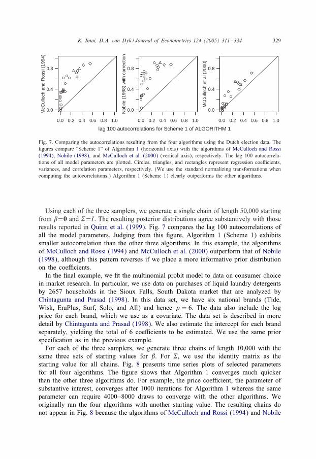
K. Imai, D.A. van Dyk / Journal of Econometrics 124 (2005) 311–334 329M
cCul
loch
and
Ros
si (
1994
)
0.0 0.2 0.4 0.6 0.8 1.0
0.0
0.4
0.8
Nob
ile (
1998
) w
ith c
orre
ctio
n0.0 0.2 0.4 0.6 0.8 1.0
0.0
0.4
0.8
McC
ullo
ch e
t al (
2000
)
0.0 0.2 0.4 0.6 0.8 1.0
0.0
0.4
0.8
lag 100 autocorrelations for Scheme 1 of ALGORITHM 1
Fig. 7. Comparing the autocorrelations resulting from the four algorithms using the Dutch election data. The0gures compare “Scheme 1” of Algorithm 1 (horizontal axis) with the algorithms of McCulloch and Rossi(1994), Nobile (1998), and McCulloch et al. (2000) (vertical axis), respectively. The lag 100 autocorrela-tions of all model parameters are plotted. Circles, triangles, and rectangles represent regression coeFcients,variances, and correlation parameters, respectively. (We use the standard normalizing transformations whencomputing the autocorrelations.) Algorithm 1 (Scheme 1) clearly outperforms the other algorithms.
Using each of the three samplers, we generate a single chain of length 50,000 startingfrom �=0 and �=I . The resulting posterior distributions agree substantively with thoseresults reported in Quinn et al. (1999). Fig. 7 compares the lag 100 autocorrelations ofall the model parameters. Judging from this 0gure, Algorithm 1 (Scheme 1) exhibitssmaller autocorrelation than the other three algorithms. In this example, the algorithmsof McCulloch and Rossi (1994) and McCulloch et al. (2000) outperform that of Nobile(1998), although this pattern reverses if we place a more informative prior distributionon the coeFcients.In the 0nal example, we 0t the multinomial probit model to data on consumer choice
in market research. In particular, we use data on purchases of liquid laundry detergentsby 2657 households in the Sioux Falls, South Dakota market that are analyzed byChintagunta and Prasad (1998). In this data set, we have six national brands (Tide,Wisk, EraPlus, Surf, Solo, and All) and hence p = 6. The data also include the logprice for each brand, which we use as a covariate. The data set is described in moredetail by Chintagunta and Prasad (1998). We also estimate the intercept for each brandseparately, yielding the total of 6 coeFcients to be estimated. We use the same priorspeci0cation as in the previous example.For each of the three samplers, we generate three chains of length 10,000 with the
same three sets of starting values for �. For �, we use the identity matrix as thestarting value for all chains. Fig. 8 presents time series plots of selected parametersfor all four algorithms. The 0gure shows that Algorithm 1 converges much quickerthan the other three algorithms do. For example, the price coeFcient, the parameter ofsubstantive interest, converges after 1000 iterations for Algorithm 1 whereas the sameparameter can require 4000–8000 draws to converge with the other algorithms. Weoriginally ran the four algorithms with another starting value. The resulting chains donot appear in Fig. 8 because the algorithms of McCulloch and Rossi (1994) and Nobile

330 K. Imai, D.A. van Dyk / Journal of Econometrics 124 (2005) 311–334
0 2000 4000 6000 8000 10000
-80
-60
-40
-80
-60
-40
iteration
pric
e co
effic
ient
-80
-60
-40
pric
e co
effic
ient
-80
-60
-40
pric
e co
effic
ient
0 2000 4000 6000 8000 10000
iteration
pric
e co
effic
ient
0 2000 4000 6000 8000 10000
-1.0
0.0
1.0
2.0
iteration
log(
σ 55)
-1.0
0.0
1.0
2.0
log(
σ 55)
-1.0
0.0
1.0
2.0
log(
σ 55)
-1.0
0.0
1.0
2.0
log(
σ 55)
0 2000 4000 6000 8000 10000iteration
0 2000 4000 6000 8000 10000
-1
1
3
5
iteration
log(
(1+
ρ 45)
/(1
−ρ 4
5))
-1
1
3
5
log(
(1+
ρ 45)
/(1
−ρ 4
5))
-1
1
3
5
log(
(1+
ρ 45)
/(1
−ρ 4
5))
-1
1
3
5
log(
(1+
ρ 45)
/(1
−ρ 4
5))
0 2000 4000 6000 8000 10000
iteration
ALGORITHM 1 (Scheme 1) McCulloch et al. (2000)
0 2000 4000 6000 8000 10000iteration
0 2000 4000 6000 8000 10000iteration
0 2000 4000 6000 8000 10000iteration
0 2000 4000 6000 8000 10000iteration
0 2000 4000 6000 8000 10000iteration
0 2000 4000 6000 8000 10000iteration
McCulloch and Rossi (1994) Nobile (1998) with correction
Fig. 8. Time series plots of the draws of selected parameters using the four algorithms to 0t the detergentbrand choice data. The 0gure shows the three chains for the price coeFcient, a variance parameter, anda correlation coeFcient. Algorithm 1 converges much faster than the algorithms of Nobile (1998) (withcorrection), McCulloch and Rossi (1994), and McCulloch et al. (2000).

K. Imai, D.A. van Dyk / Journal of Econometrics 124 (2005) 311–334 331
(1998) were extremely slow to converge, taking about 60,000 and 80,000 draws, respec-tively, to converge. Even with this starting value, our algorithm again converged in un-der 1000 draws. In terms of the autocorrelations of the draws upon convergence in thisexample, Algorithm 1 performs better than the algorithm of McCulloch et al. (2000)and about the same as the algorithms of McCulloch and Rossi (1994) and Nobile(1998).
6. Concluding remarks
When comparing statistical methods, computational performance should nearly al-ways be a less important criterion than the choice of model speci0cation. In the con-text of the multinomial probit model, we expect methods which place a prior dis-tribution directly on the identi0able parameters to be easier to use and more readilyable to reNect available prior information in practice. Thus, we agree completely withthe approach of McCulloch et al. (2000), which sacri0ces computational eFciency inorder to accommodate a more attractive model speci0cation. Of course, as some ofthe examples is McCulloch et al. (2000) illustrate, in extreme cases computationalconcerns can render a model practically untenable. In some fortunate situations, how-ever, algorithms exist that allow for attractive model speci0cations while also main-taining eFcient computation. As has been demonstrated in the literature, the methodof marginal augmentation is a useful tool for 0nding such algorithms. Thus, this arti-cle uses marginal augmentation to accomplish what Nobile (2000) hoped for when heremarked,
Perhaps some ingenuity is needed to devise a sampling Markov chain which uses[the prior of McCulloch et al. (2000)] and has good mixing properties.
Although our prior distribution is not that of McCulloch et al. (2000), in termsof each of the three criteria used to compare the algorithms in Table 1, we believethe algorithms we recommend are equal to the best available methods. We specify aneasy-to-use prior distribution on the identi0able model parameters and our algorithmsrequire only draws from standard distributions. In our numerical comparisons, theseadvantages come without computational cost; overall the performance of the methodswe recommend is better than any other method in terms of both autocorrelation andinsensitivity to starting values. It would seem that sometimes there is such a thing asa free lunch!
Acknowledgements
The authors gratefully acknowledge funding for this project partially provided byNSF Grant DMS-01-04129, the U.S. Census Bureau, and by the Princeton UniversityCommittee on Research in the Humanities and Social Sciences. The 0rst author thanksGary King for his continuous encouragement.

332 K. Imai, D.A. van Dyk / Journal of Econometrics 124 (2005) 311–334
Appendix A. Details of two new algorithms
In this Appendix, we give details of Algorithms 1 and 2 for the multinomial pro-bit model. We begin with Algorithm 1 with starting value � (0) = (�(0); �(0)) and for“Scheme 2,” �(0) = 1 and proceed via the following three steps at iteration t:
Algorithm 1. Step 1: For each i and each j=1; : : : ; p−1 draw W ∗ij given W ∗
i;−j; �(t−1),
and Y , where
W ∗i;−j = (W ∗
i1; : : : ; W∗i; j−1; W
(t−1)i; j+1 ; : : : ; W
(t−1)i;p−1) (A.1)
exactly as described in Section 3 of McCulloch and Rossi (1994). (McCulloch andRossi (1994) use the symbols � and � for the unidenti$ed parameters, i.e., our � and�. In this step W ∗ should be generated using the identi$ed parameters, so notationallythis is equivalent to McCulloch and Rossi (1994).) For “Scheme 1” draw (�2)∗ fromp(�2 | �; �) = p(�2 |�) as given in (6) and set W ∗
ij = �∗W ∗ij . For “Scheme 2” set
W ∗ij = �(t−1)W ∗
ij .Step 2: Draw �∗ and (�2)∗ given W ∗ and �(t−1),
(�2)∗ ∼ {∑ni= 1(W
∗i −Xi�)�(�(t−1))−1(W ∗
i −Xi�) + ��A�+trace[S(�(t−1))−1]}�2(n+�)(p−1)
;
(A.2)
where
�=
[n∑i=1
X�i (�(t−1))−1Xi + A
]−1 [ n∑i=1
X�i (�(t−1))−1W ∗
i
];
�∗ ∼ N
�; (�2)∗
(n∑i=1
X�i (�(t−1))−1Xi + A
)−1 ; (A.3)
and set �(t) = �∗=�∗.Step 3: Finally, draw �(t) given �(t) and (W ∗
i − Xi�∗), for i = 1; : : : ; n via
�∗ ∼ InvWishart
[n+ �; S +
n∑i=1
(W ∗i − Xi�∗)(W ∗
i − Xi�∗)�]; (A.4)
set �(t) = �∗=�∗11 and W (t)
ij = W ∗ij=√�∗11 for each i and j, and for “Scheme 2” set
(�2)(t) = �∗11.
Here, superscript stars indicate quantities that are intermediate and not part of theMarkov chain, (W (t); �(t); �(t)) and (W (t); �(t); �(t); �(t)) for “Scheme 1” and “Scheme2”, respectively.
We now give the details of Algorithm 2.

K. Imai, D.A. van Dyk / Journal of Econometrics 124 (2005) 311–334 333
Algorithm 2. Step 1a: Draw W ∗ij just as in Step 1 of Algorithm 1. Then draw (�2)∗
from p(�2 | �; �) = p(�2 |�) as given in (6) and set W ∗ij = �∗(W ∗
ij − Xi�(t−1)).Step 1b: Draw �∗ given W ∗ and �(t−1),
�∗ ∼ InvWishart
[n+ �; S +
n∑i=1
W ∗i (W
∗i )
�]; (A.5)
and set �(t) = �∗=�∗11.
Step 1c: Set
W (t)i =
1√�∗11
W ∗i + Xi�(t−1) for each i: (A.6)
Step 2: Finally, draw �(t) given �(t) and W (t)
�(t) ∼ N
�;
(n∑i=1
X�i (�(t))−1Xi + A
)−1 ; (A.7)
where
� =
[n∑i=1
X�i (�(t))−1Xi + A
]−1 [ n∑i=1
X�i (�(t))−1W (t)
i + A�0
]:
(Again superscript stars are used to indicate intermediate quantities.)
Appendix B. Nobile’s Metropolis–Hastings acceptance rate
To compute the correct acceptance rate for Nobile’s (1998) Metropolis–Hastingsrule, we 0rst derive the target distribution,
p(� | �; �)˙ p(�; �; �) (B.1)
˙ �−(�(p−1)−k+1) exp{
−12
[(�� − �0)�A(�� − �0)
+1�2
trace(S�−1)]}
: (B.2)
Thus,
R=p(�′ | �; �)p(� | �; �)
J (� | �′)J (�′ | �)
= exp{
−12
[�2��A�(c2−1)−2���
0 A�(c−1)+1�2
trace(S�−1)(
1c2
−1)]}
× c−(�(p−1)−k+2) exp(c − 1
c
); (B.3)
where c= �′=�. This diKers from the value computed by Nobile (1998) by a factor ofc−(2−k−p(p−1)=2).

334 K. Imai, D.A. van Dyk / Journal of Econometrics 124 (2005) 311–334
References
Ben-Akiva, M.E., Lerman, S.R., 1985. Discrete Choice Analysis: Theory and Application to Travel Demand..MIT Press, Cambridge, MA.
Chib, S., Greenberg, E., Chen, Y., 1998. MCMC methods for 0tting and comparing multinomial responsemodels. Economics Working Paper Archive, Econometrics, No. 9802001, Washington University atSt. Louis.
Chintagunta, P.K., Prasad, A.R., 1998. An empirical investigation of the “Dynamic McFadden” model ofpurchase timing and brand choice: implications for market structure. Journal of Business and EconomicStatistics 16 (1), 2–12.
Cowles, M.K., Carlin, B.P., 1996. Markov chain Monte Carlo convergence diagnostics: a comparative review.Journal of the American Statistical Association 91, 883–904.
Gelman, A., Rubin, D.B., 1992. Inference from iterative simulations using multiple sequences (withdiscussion). Statistical Science 7, 457–472.
Geweke, J., Keane, M., Runkle, D., 1994. Alternative computational approaches to inference in themultinomial probit model. The Review of Economics and Statistics 76, 609–632.
Haas, M., 1998. Value of IgG subclasses and ultrastructural markers in predicting latent membranous lupusnephritis. Modern Pathology 11, 147A.
Hausman, J.A., Wise, D.A., 1978. A conditional probit model for qualitative choice: discrete decisionsrecognizing interdependence and heterogeneous preferences. Econometrica 46, 403–426.
Keane, M.P., 1992. A note on identi0cation in the multinomial probit model. Journal of Business andEconomic Statistics 10, 193–200.
Liu, J.S., Wong, W.H., Kong, A., 1994. Covariance structure of the Gibbs sampler with applications tocomparisons of estimators and augmentation schemes. Biometrika 81, 27–40.
Maddala, G., 1983. Limited-dependent and Qualitative Variables in Econometrics. Cambridge UniversityPress, Cambridge.
McCulloch, R., Rossi, P., 1994. An exact likelihood analysis of the multinomial probit model. Journal ofEconometrics 64, 207–240.
McCulloch, R., Rossi, P., 2000. Reply to Nobile. Journal of Econometrics 99, 347–348.McCulloch, R., Polson, N.G., Rossi, P., 2000. A Bayesian analysis of the multinomial probit model with
fully identi0ed parameters. Journal of Econometrics 99, 173–193.Meng, X.-L., van Dyk, D.A., 1999. Seeking eFcient data augmentation schemes via conditional and marginal
augmentation. Biometrika 86, 301–320.Nobile, A., 1998. A hybrid Markov chain for the Bayesian analysis of the multinomial probit model. Statistics
and Computing 8, 229–242.Nobile, A., 2000. Comment: Bayesian multinomial probit models with normalization constraint. Journal of
Econometrics 99, 335–345.Quinn, K.M., Martin, A.D., Whitford, A.B., 1999. Voter choice in multi-party democracies: a test of
competing theories and models. American Journal of Political Science 43, 1231–1247.Roberts, G.O., 1996. Markov chain concepts related to sampling algorithms. In: Gilks, W.R., Richardson,
S., Spiegelhalter, D.J. (Eds.), Markov Chain Monte Carlo in Practice. Chapman & Hall, London.Speckman, P.L., Lee, J., Sun, D., 1999. Existence of the MLE and propriety of posteriors for a general
multinomial choice model. Technical Report, Department of Statistics, University of Missouri at Columbia.Tanner, M.A., Wong, W.H., 1987. The calculation of posterior distributions by data augmentation (with
discussion). Journal of the American Statistical Association 82, 528–550.Tierney, L., 1994. Markov chains for exploring posterior distributions (with discussion). The Annals of
Statistics 22, 1701–1762.Tierney, L., 1996. Introduction to general state-space markov chain theory. In: Gilks, W.R., Richardson, S.,
Spiegelhalter, D.J. (Eds.), Markov Chain Monte Carlo in Practice. Chapman & Hall, London.van Dyk, D.A., Meng, X.-L., 2001. The art of data augmentation (with discussions). The Journal of
Computational and Graphical Statistics 10, 1–111.van Dyk, D.A., Kang, H., Meng, X.-L., 2004. Using a marginal gibbs sampler to improve bayesian
computation for the glmm. Technical Report.