Seediscussions,stats,andauthorprofilesforthispublicationat:https://www.researchgate.net/publication/307999719

ABiologicallyInspiredFrameworkforVisualInformationProcessingandanApplicationonModelingBottom-UpVisual...

ArticleinCognitiveComputation·September2016

DOI:10.1007/s12559-016-9430-8

CITATIONS

0

READS

99

3authors:

Someoftheauthorsofthispublicationarealsoworkingontheserelatedprojects:

TagsnetworkViewproject

TRM104-SUSIE+Viewproject

AlaAboudib

InstitutMines-Télécom

7PUBLICATIONS17CITATIONS

SEEPROFILE

VincentGripon

InstitutMines-Télécom

74PUBLICATIONS398CITATIONS

SEEPROFILE

GillesCoppin

TelecomBretagne/Lab-STICCUMR6285

82PUBLICATIONS167CITATIONS

SEEPROFILE

AllcontentfollowingthispagewasuploadedbyAlaAboudibon15September2016.

Theuserhasrequestedenhancementofthedownloadedfile.Allin-textreferencesunderlinedinblueareaddedtotheoriginaldocumentandarelinkedtopublicationsonResearchGate,lettingyouaccessandreadthemimmediately.

Noname manuscript No.(will be inserted by the editor)

A biologically-inspired framework for visualinformation processing and an application onmodeling bottom-up visual attention

Ala Aboudib · Vincent Gripon · GillesCoppin

Received: date / Accepted: date

Abstract An emerging trend in visual information processing is toward incor-porating some interesting properties of the ventral stream in order to accountfor some limitations of machine learning algorithms. Selective attention andcortical magnification are two such important phenomena that have been thesubject of a large body of research in recent years. In this paper, we proposea new framework for visual information acquisition and representation thatemulates the architecture of the primate visual system by integrating featuressuch as retinal sampling and cortical magnification while avoiding spatial de-formations and other side effects produced by current models that tried toimplement these two features. It also explicitly integrates the notion of visualangle, which is rarely taken into account by vision models. We argue thatthis framework can provide the infrastructure for implementing vision taskssuch as object recognition and computational visual attention algorithms. Italso raises important questions about the role of the newly integrated fea-tures on vision behavior. Moreover, we propose an algorithm for bottom-upvisual attention implemented using the proposed framework, and show thatit can attain state-of-the-art performance, and provide a better insight on thesignificance of studying the role of the visual angle more closely.

Keywords cortical magnification · bottom-up attention · saliency · retinalsampling · foveation

This work was supported by the European Research Council under the European Union’sSeventh Framework Program (FP7/2007-2013) / ERC grant agreement n◦ 290901.

Telecom BretagneTechnopole Brest-Iroise, CS 83818 – 29238 Brest cedex 3, FranceLab-STICC UMR CNRS 6285Email addresses: {name}.{surname}@telecom-bretagne.eu

4 Ala Aboudib et al.

1 Introduction

Vision and the visual system have been an active area of research for manycenturies. Interest in exploring this territory has been motivated by a widevariety of applications. Ophthalmology was one of the first domains to benefitfrom such discoveries. More recently, that interest has been widely driven bythe desire to learn more about the brain and decipher its neural code. A betterunderstanding of the neural code has enabled to design better machine learningalgorithms for computer vision, and for artificial intelligence in a more generalsense.

The discovery of simple and complex cells in the famous work by Hubel andWiesel on receptive fields in the cat’s visual cortex (Hubel and Wiesel, 1959)marked a new era in vision research. It revolutionized the way the visual systemis studied and understood, and allowed for the emergence of ‘computationalneuroscience’, a new field founded by David Marr whose theory on vision isstill very influential (Marr, 1982).

More recently, deep learning networks have achieved an unprecedentedperformance on many visual tasks such as image categorization (Krizhevskyet al, 2012). The architecture of these networks has been inspired by the multi-layered structure of the visual system and the hierarchical organization ofsimple and complex cells.

Some criticism of deep learning includes its limited performance on taskssuch as unsupervised object discovery and localization, multiple instance recog-nition (MIL) (Zhu et al, 2015; Ray et al, 2010), recognizing spatial relationshipsbetween objects and its limited ability to generalizing to variable-scale repre-sentations of the learned classes without increasing the size of the trainingset (Lake et al, 2015). Another important problem of deep learning, accordingto (Ranzato et al, 2015), is its computational cost, which renders it impracticalfor very high resolution images. This called some researchers to get a closerlook at the visual system and some of its overlooked properties to addressthese limitations.

One such property is selective visual attention that guides covert processingbiases and saccadic eyes movements. The study of this property is an emergingtrend in visual information processing. It finds its root in Treisman’s FeatureIntegration Theory (FIT) (Treisman and Gelade, 1980). This theory provideda strong evidence of the fundamental role of attention for object recognition.This role was later explored by many researchers including (Koch and Ullman,1987; Itti et al, 1998; Walther et al, 2004; Bonaiuto and Itti, 2005; Borji et al,2014). It also motivated the recent emergence of attention-based recognitionas in (Larochelle and Hinton, 2010; Zheng et al, 2015).

Cortical magnification is another ubiquitous feature of the visual system(Gattass et al, 1981, 1988). In addition to its role in reducing the amount ofvisual information entering the brain, Poggio has proposed that it might be akey property for enabling scale-invariant learning of objects (Isik et al, 2011;Anselmi et al, 2015).

Title Suppressed Due to Excessive Length 5

In this paper, we propose a new framework for visual information acquisi-tion that integrates these important features of the ventral stream. Our con-tributions are the following:

1. Introducing a new bio-inspired framework for visual information acquisi-tion and representation that offers the following properties:

– Providing a method for taking the distance between an image and theviewer into account. This is done by incorporating a visual angle pa-rameter which is ignored by most visual acquisition models.

– Reducing the amount of visual information acquired by introducing anew scheme for emulating retinal sampling and the cortical magnifica-tion effects observed in the ventral stream.

2. Providing a concrete application of the proposed framework by using itas a substrate for building a new saliency-based visual attention model,which is shown to attain state-of-the-art performance on the MIT saliencybenchmark (Borji et al, 2013a).

3. Providing an online Git repository that implements the introduced frame-work that is meant to be developed as a scalable, collaborative project.

The rest of this paper is organized as follows: In Section 2, related workis reviewed. Section 3 introduces a brief anatomy of the visual system and itsfunction, paving the way to Section 4 where a new vision framework is proposedthat captures some interesting properties of the visual system. In Section 5,a new model of visual attention is proposed using the proposed framework.We show in Section 6 that coupling the proposed vision framework with theproposed attention model gives interesting results that motivates the utility ofthe framework. A discussion of some of the model’s properties is also discussedin Section 6. Section 7 is a conclusion.

2 Related Work

Computational and mathematical modeling of the visual system have been thefocus of many works in literature in recent years. The scope of such modelsincludes mathematical models of single neurons (McCulloch and Pitts, 1943),neural assemblies through sparse coding techniques (Lee et al, 2006; Liu et al,2015) and receptive field models (Rodieck, 1965; Marcelja, 1980) or even mod-eling complete visual layers, especially the retina (Wohrer and Kornprobst,2009) or successions of layers representing early areas of the visual cortex suchas in the Hmax model (Serre et al, 2007) or in the one proposed by DavidMarr in his famous work on vision (Marr, 1982).

Most vision models are designed to accomplish a specific task. For in-stance, the Hmax model is a view-based object recognition processor. It isinspired by the description of simple and complex cells in the primary visualcortex by Hubel and Wiesel (Hubel and Wiesel, 1962). A similar model wasproposed in (LeCun et al, 1998), which also provides an implementation ofsimple and complex cells. However, it uses supervised learning coupled with

6 Ala Aboudib et al.

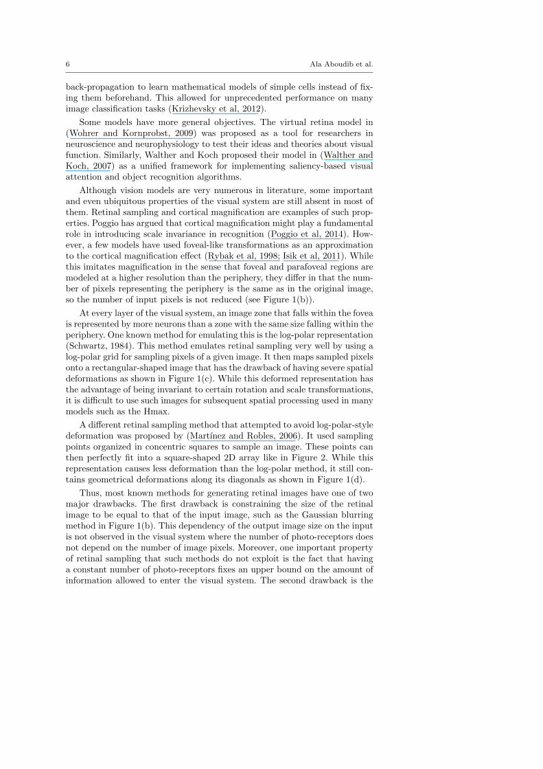
back-propagation to learn mathematical models of simple cells instead of fix-ing them beforehand. This allowed for unprecedented performance on manyimage classification tasks (Krizhevsky et al, 2012).

Some models have more general objectives. The virtual retina model in(Wohrer and Kornprobst, 2009) was proposed as a tool for researchers inneuroscience and neurophysiology to test their ideas and theories about visualfunction. Similarly, Walther and Koch proposed their model in (Walther andKoch, 2007) as a unified framework for implementing saliency-based visualattention and object recognition algorithms.

Although vision models are very numerous in literature, some importantand even ubiquitous properties of the visual system are still absent in most ofthem. Retinal sampling and cortical magnification are examples of such prop-erties. Poggio has argued that cortical magnification might play a fundamentalrole in introducing scale invariance in recognition (Poggio et al, 2014). How-ever, a few models have used foveal-like transformations as an approximationto the cortical magnification effect (Rybak et al, 1998; Isik et al, 2011). Whilethis imitates magnification in the sense that foveal and parafoveal regions aremodeled at a higher resolution than the periphery, they differ in that the num-ber of pixels representing the periphery is the same as in the original image,so the number of input pixels is not reduced (see Figure 1(b)).

At every layer of the visual system, an image zone that falls within the foveais represented by more neurons than a zone with the same size falling within theperiphery. One known method for emulating this is the log-polar representation(Schwartz, 1984). This method emulates retinal sampling very well by using alog-polar grid for sampling pixels of a given image. It then maps sampled pixelsonto a rectangular-shaped image that has the drawback of having severe spatialdeformations as shown in Figure 1(c). While this deformed representation hasthe advantage of being invariant to certain rotation and scale transformations,it is difficult to use such images for subsequent spatial processing used in manymodels such as the Hmax.

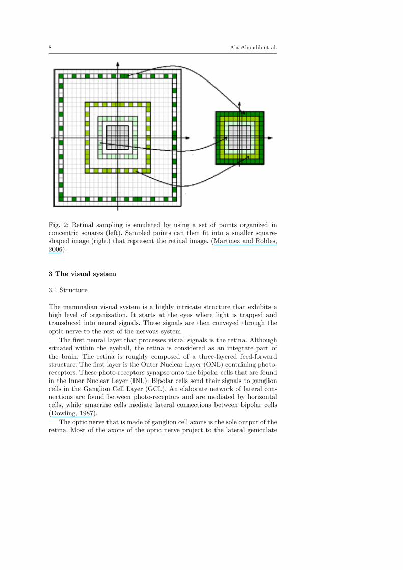
A different retinal sampling method that attempted to avoid log-polar-styledeformation was proposed by (Martınez and Robles, 2006). It used samplingpoints organized in concentric squares to sample an image. These points canthen perfectly fit into a square-shaped 2D array like in Figure 2. While thisrepresentation causes less deformation than the log-polar method, it still con-tains geometrical deformations along its diagonals as shown in Figure 1(d).

Thus, most known methods for generating retinal images have one of twomajor drawbacks. The first drawback is constraining the size of the retinalimage to be equal to that of the input image, such as the Gaussian blurringmethod in Figure 1(b). This dependency of the output image size on the inputis not observed in the visual system where the number of photo-receptors doesnot depend on the number of image pixels. Moreover, one important propertyof retinal sampling that such methods do not exploit is the fact that havinga constant number of photo-receptors fixes an upper bound on the amount ofinformation allowed to enter the visual system. The second drawback is the

Title Suppressed Due to Excessive Length 7

(a) Original image. (b) Blurring.

(c) Log-polar. (d) Square-sampling.

Fig. 1: Some of the classical methods traditionally used for emulating retinalsampling and cortical images. Notice that blurring in (b) keeps the same num-ber of pixel as in the original image. The log-polar and the square-samplingmethods in (c) and (d) introduce severe spatial deformations that make furtherspatial filtering more challenging.

deformation introduced by methods that try to avoid the first drawback as inFigures 1(d) and (c).

We think that the main reason why such methods always have one ofthe above drawbacks is that they are constrained to producing an outputimage with a ‘regular’ shape. The term ‘regular’ here means a circular or arectangular shape. This constraint is set such that the output image is suitablefor presentation to a human observer or to be compatible with available imageprocessing tools.

In the vision framework we propose in Section 4, no such shape constraintsare fixed. Hence, we introduce a simple method for applying cortical magnifica-tion and retinal sampling in which the output is completely independent fromthe size of the input image without producing any geometrical deformations.

8 Ala Aboudib et al.

Fig. 2: Retinal sampling is emulated by using a set of points organized inconcentric squares (left). Sampled points can then fit into a smaller square-shaped image (right) that represent the retinal image. (Martınez and Robles,2006).

3 The visual system

3.1 Structure

The mammalian visual system is a highly intricate structure that exhibits ahigh level of organization. It starts at the eyes where light is trapped andtransduced into neural signals. These signals are then conveyed through theoptic nerve to the rest of the nervous system.

The first neural layer that processes visual signals is the retina. Althoughsituated within the eyeball, the retina is considered as an integrate part ofthe brain. The retina is roughly composed of a three-layered feed-forwardstructure. The first layer is the Outer Nuclear Layer (ONL) containing photo-receptors. These photo-receptors synapse onto the bipolar cells that are foundin the Inner Nuclear Layer (INL). Bipolar cells send their signals to ganglioncells in the Ganglion Cell Layer (GCL). An elaborate network of lateral con-nections are found between photo-receptors and are mediated by horizontalcells, while amacrine cells mediate lateral connections between bipolar cells(Dowling, 1987).

The optic nerve that is made of ganglion cell axons is the sole output of theretina. Most of the axons of the optic nerve project to the lateral geniculate

Title Suppressed Due to Excessive Length 9

nucleus (LGN) in the thalamus. An important part of axons in the optic nervealso project to the superior colliculus. The optic nerve is the first stream wherevisual signals take the form of action potentials. Action potentials conveyedto the LGN by the optic nerve continue their way through the optic radiationwhich is another axonal structure. The optic radiation projects to the primaryvisual cortex V1 in the occipital lobe (Hubel and Wiesel, 1962).

The occipital lobe is divided into two distinct layers called V1 and V2. Theoptic radiation coming from LGN terminates in V1. At this point and startingfrom V2, the visual stream starts to diverge into to two distinct pathways:the ventral and the dorsal pathways. It has been argued that these pathwaysact as two independent visual systems with distinct functions (Goodale andMilner, 1992): the ‘What’ and the ‘Where’ systems. The ‘What’ system issituated in the temporal lobe. It is responsible for visual recognition taskssuch as recognizing the identity of faces and other objects. In this system,higher visual areas such as V4, PIT, CIT and AIT are found. The ‘Where’system, sometimes called the ‘How’ system, is found in the parietal lobe. It hasbeen suggested that visually-guided behavior, such as reaching and grasping,is among the main functions of this system. Higher visual areas such as MT,LIP, MST and VIP are parts of this system. However, A later work by (Milnerand Goodale, 2008) suggested the existence of a more complex interactionscheme than a simple separation into two independent systems.

It is worth pointing out that, in addition to the feed-forward pathway ofaxons, a rich feedback stream also go down throughout all the stages describedso far.

3.2 Function

Two major families of photo-receptors are found in ONL: rods and cones.Rods are sensitive to low light conditions and are mainly responsible for nightvision. On the other hand, cones are less sensitive to light, which makes themmore adapted to day vision when light is abundant. Rods’ and cones’ mainfunction is to transduce incoming photons into neural signals. These signalsare further processed by the network of horizontal, bipolar and amacrine cells.They finally arrive at ganglion cells which translate them into action potentialsand send them via the optic nerve to other areas.

There are two major types of ganglion cells with distinct functions, Parasoland midget cells. Parasol cells, also called M,Y or β cells, have wider recep-tive fields (RFs). They are characterized by a lower spatial resolution and atransient response to persistent stimuli. They are associated with achromaticvision. On the other hand, midget cells, which are sometimes called P, X orα cells, have smaller RFs. They have a higher spatial resolution and a lowertemporal resolution than parasol cells, and they are associated with color vi-sion. Each type of the above ganglion cells is divided into two sub-types calledON or OFF cells, which have complementary response levels. Hence, we find

10 Ala Aboudib et al.

parasol-ON, parasol-OFF, midget-On and midget-OFF cells (Salin and Bul-lier, 1995; Hubel and Wiesel, 1959).

Most ganglion cells are known for their center-surround configuration. ONganglion cells are excited by the onset of light stimuli in their central regionand inhibited by light in their surround region. The inverse holds for OFFganglion cells. Rodieck was the first to propose an elegant mathematical modelfor spatial and temporal responses of ganglion cells in the form a difference ofGaussians (DoG) (Rodieck, 1965). This center-surround model is also involvedin color vision. For example, some midget-ON cells encode the degree of red intheir RFs; their center is excited by long wave (red) light and their surroundis inhibited by medium wave (green) light. Another type is sensitive to blue,having a center excited by short wave (blue) light and a surround inhibited bymedium and long wave light.

Neurons in higher visual areas respond to progressively more complex stim-ulus patterns. In the primary visual cortex V1, for example, neurons are tunedto simple oriented contours and spatial frequencies. The response of V1 cells,also called simple cells by (Hubel and Wiesel, 1959), are typically modeledmathematically by a Gabor filtering process, which consists in convoluting animage with a Gabor kernel made of the product of a 2D Gaussian kernel by a2D cosine grating. Some neurons in V2 respond to stimuli as simple as orientededges, but they are also tuned to illusory edges and a slightly more complexshapes. However, the complexity of spatial and temporal response patterns ofneurons grows in complexity in higher visual areas.

3.3 Information reduction

The visual field (VF) of a single eye spans about 160◦ horizontally and 174◦

vertically. While a tremendous amount of visual information could be extractedfrom such a wide span, the visual system uses intelligent tricks to reduce theamount of acquired information. This reduction starts as early as the ONLlayer in the retina; the visual field is sampled by the photo-receptors in anon-uniform fashion. The density of cones is very high in the central region ofthe retina called the fovea, spanning about 1◦, and decreases logarithmicallytoward the periphery as shown in Figure 3. This distribution leads to what iscalled ‘retinal sampling’ (Salin and Bullier, 1995; Hubel and Wiesel, 1959).

The reduction of visual information by means of a ‘privileged’ fovea con-tinues in subsequent areas of the visual system. For example, among ganglioncells of the same type, those which pool their inputs from photo-receptorsnear the fovea have smaller receptive fields than cells pooling their inputsfrom photo-receptors in the periphery. This phenomenon is known as the cor-tical magnification effect. This effect is also observed in LGN, V1, V2, V4 andeven in higher visual areas. The ratio between the diameter of a given RF andits eccentricity stays relatively constant in a given visual layer and increasesin higher areas as shown in Figure 4.

Title Suppressed Due to Excessive Length 11

Fig. 3: Spatial density distribution of rods and cones in the retina (Gonzalezand Woods, 2002).

4 The proposed vision framework

In this section, we propose a model for visual information acquisition and rep-resentation in early layers of the visual system. This model is meant to be usedas a framework for implementing visual processing tasks such as visual atten-tion modeling presented in section 5, or object recognition algorithms thatneed hierarchical information processing. This model imitates the informationreduction property of the visual system described in Section 3. It does this byemulating retinal sampling and the cortical magnification effect. This leads tosome interesting properties discussed later in Section 6.

As we have seen in section 3, the early visual system can be functionallyviewed as an arrangement of consequent layers. It starts at the photo-receptorlayer (ONL) in the retina and continues through the GCL layer, the LGN, V1,V2 and so on. The transition from one layer into another can be viewed as amapping mediated by synaptic connections constituting receptive fields.

The model we propose is made of two basic components: visual layersmodeled as point clouds, and mapping functions between these layers in thefeed-forward direction.

4.1 Notation

In this paper, polar coordinates and their corresponding Cartesian coordinatesare sometimes used interchangeably depending on the context. The radial com-ponent of a polar coordinate is always denoted by the roman letter r, while

12 Ala Aboudib et al.

Fig. 4: Cortical magnification factors in V1, V2 and V4 adapted from (Gattasset al, 1981) and (Gattass et al, 1988) by (Freeman and Simoncelli, 2011).

the angle is denoted by the Greek letter ω. The Cartesian version of (r,ω) isalways denoted by (x, y), where x = r cosω and y = r sinω. If polar coor-dinates are written with super- and/or subscripts, these same super- and/orsubscripts are attached to their Cartesian versions, and vice versa.

4.2 A generic model for visual layers

Visual layers as well as input stimuli are modeled as point clouds using a setrepresentation. This representation can be used to instantiate any number oflayers, which is a variable parameter between vision models, by providing ageneric description that captures common properties of layers in the visualsystem as well as input stimuli, such as the visual field spanned by a layer,its fovea size, spatial distribution of cells and the distribution of associatedreceptive fields.

However, this representation focuses on two main properties of the vi-sual system. First, it is adapted to implementing the information reductionproperties in the form of retinal sampling and cortical magnification withoutintroducing any deformations. Second, it implements the notion of visual anglewhich determines the visual field span associated with a given layer. The latterproperty is one main difference between the vision framework we propose andthe one proposed in (Walther and Koch, 2007).

Hence, the structure of a given visual layer can be captured by our modelusing the following generic definition:

Title Suppressed Due to Excessive Length 13

C(Θc,ψc,Dc) = {f ck |f c

k : R2 → R,

σ(diam(dom(f ck))) = Θc,

k ∈ {1, ...,Kc}}, (1)

where dom(f ck) represents the domain of function f c

k , which is the set of pointsinR2 on which f c

k is defined, e.g., the coordinates of points in Figure 5, the termdiam(dom(f c

k)) refers to the diameter of the set dom(f ck), e.g., the diameter

of point clouds in Figure 5, and σ(diam(dom(f ck))) is the the visual angle Θc

spanned by that diameter. Similarly, ψc is the visual angle spanned by thediameter of a central subset of dom(f c

k) called the fovea. The parameter Dc isused to specify a two dimensional spatial distribution of points in dom(f c

k).

(a)(b)

Fig. 5: Two example point clouds representing visual layers according to thedefinition in (1). A different distribution Dc is used for each cloud. In (a), thedistribution Dc is chosen as a regular grid. This distribution is more adapted torepresenting images with a classical rectangular shape. In (b), this distributionis chosen at random. This shows that the representation of visual layers in theproposed framework is not limited to rectangular distributions as in mostvision models.

As an illustrative example, the definition in (1) can be used to representa classical two dimensional RGB image. In this case, the distribution Dc ischosen as a 2D rectangular grid corresponding to pixel positions of the imageas in Figure 5 (a), k refers to an image component (R, G or B) and fc

k is thevalue of the component k at an index (i, j) in N2.

An interesting feature of using C to represent an image is that it associatesa visual angle Θc with its diagonal. This emulates the fact that, in reality,an image is always associated with a certain visual angle when viewed froma certain distance. We argue that this is an important element for any model

14 Ala Aboudib et al.

that aims at a faithful modeling of the visual systems. It allows to study theinfluence of the visual angle on the behavior of models performing visual tasks.

The cone receptors layer in the ONL can also be modeled using the defini-tion in (1). In this case, Dc would be chosen to approximate cone distributionin the retina shown in Figure 3. This means that the density of points indom(f c

k) would be higher in the foveal region defined by ψc, and decreaselogarithmically towards the periphery. Each point fc

k would represent a conereceptor whose type would be determined by the subscript k (a S, M or Lcone). The angles Θc and ψc would represent the layer’s visual field and thewidth of the fovea in degrees of visual angles, respectively.

In a much similar way to representing a cone-receptors layer, other visuallayers such as the ganglion cell layer in the retina, LGN, V1 and higher layerscan be modeled by (1) as we will see in Section 5.

An optional modulation function mc can be applied to a layer C:

mc : R|C| → R|C|. (2)

This function can be used to implement any operation that globally modi-fies values of points in a given layer. Example operations include non-linearitiessuch as contrast gain control and intensity adaptation as in the retina, the In-hibition of Return (IOR) operation used in most models of visual attention,or any other operation.

4.3 Stacking layers

In the same way as a ganglion cell pools over a number of photo-receptors(mediated by bipolar cells), or a neuron in V1 pools over a number of axonsseen by its RF in LGN to produce their output, layers of type C can bestacked to emulate the feed-forward path of the visual system. In this case,each point in a C-type layer gets its value by pooling over a set of pointsbelonging to the previous layer. More precisely, given two layers C1 and C2, apoint f c2

k (xo, yo) ∈ C2 can be associated with a set of coordinates called itsreceptive field RFc1c2(f c2

k ) ⊆ dom(f c1k ), where f c1

k ∈ C1:

RFc1c2k (f c2

k (xo, yo)) = {(x, y)|(x, y) ∈ dom(f c1k� ),

(xo, yo) ∈ dom(f c2k ),

and (x, y) satisfies some condition

guaranteeing its membership to the

receptive field of f c2k (xo, yo)}. (3)

Determining whether a coordinate (x, y) is in the receptive field of a pointf c2k (xo, yo) depends on the types of C1 and C2. For example, if both C1 and C2model cortical layers, then a typical way of determining the RF membershipis by looking whether (x, y) falls within a disk-shaped region around (xo, yo),

Title Suppressed Due to Excessive Length 15

given that (x, y) and (xo, yo) belong to the same space. When C1 is used tomodel a RGB image, and C2 models a cone-receptor layer, the process becomessimilar to retinal sampling where a point in the receptors layer gets its value bysampling only one pixel in the image. In this case, determining the receptivefield of f c2

k (xo, yo) consists in finding its corresponding point in C1.The input signal to the point fc2

k (xo, yo) can be defined as follows:

sc1c2k (f c2k (xo, yo)) = {f c1

k� (x, y)|(x, y) ∈ RFc1c2(f c2

k (xo, yo))}, (4)

and the value of f c2k (xo, yo) can be finally computed as:

f c2k (xo, yo) = φc1c2

k (sc1c2k (f c2k (xo, yo))), (5)

where φc1c2 is a mapping defined as:

φc1c2k : R|sc1c2

k (fc2k (xo,yo))| → R. (6)

This mapping can be linear as in the case of Gabor or DoG kernels. It canalso be used to implement non-linearities for pooling functions.

In the next section, we propose a model for saliency-based visual attentionthat implements the proposed vision framework. This will shed the light on theframework’s interesting properties and raises some insightful questions abouttheir role in visual processing in Section 6.

5 Application: modeling bottom-up visual attention

Many models have been proposed in litterature for modeling visual attentionin recent years. This emerging field has been the subject of a large body ofresearch in neuroscience as well as in computer vision. It has been useful inmany applications including object recognition and video compression (Borjiand Itti, 2013; Walther et al, 2004), object segmentation (Tu et al, 2016) anddetection (Pan et al, 2016; Gao et al, 2015).

The Feature Integration Theory (FIT) introduced in (Treisman and Gelade,1980) was probably the first to suggest a fundamental functional role for at-tention in visual recognition. A few years later, Koch & Ullman proposed apossible neural mechanism for driving attention (Koch and Ullman, 1987).This mechanism only considered low-level image features in which only color,intensity contrast and local intensity orientations are used to drive the focus ofattention. The first working implementation of this mechanism was proposedby Itti and Koch, and became a landmark for saliency prediction based onbottom-up visual attention (Itti et al, 1998). The term bottom-up comes fromthe fact that only basic information about the image signal such as color andintensity are involved in predicting saliency. Other models has attempted to

16 Ala Aboudib et al.

enforce bottom-up biases with higher level information about the scene suchas recognition of objects or proto-objects (Judd et al, 2009; Zhao et al, 2014),scene context and gist information (Goferman et al, 2012; Torralba et al, 2006)and by using fully convolutional neural networks more recently (Kruthiventiet al, 2015).

The algorithm we propose here is based on the model of Itti and Koch.However, it shortcuts the first two steps consisting in Gaussian sub-samplingand across-scale subtraction. These steps are replaced by a filtering operationusing kernels with eccentricity-dependent receptive fields emulating the corti-cal magnification effect. This allows us to reduce the number of feature mapsto 9 maps instead of 42 maps in the original model.

The model we propose holds some similarity to the one the authors intro-duced in (Aboudib et al, 2015) with several major differences:

– The proposed model is implemented using the vision framework proposedin Section 4.

– The proposed vision framework allows for a more plausible way for emu-lating retinal sampling and cortical magnification factors.

– Normalized feature maps are directly combined to form the final saliencymap without computing conspicuity maps.

Figure 6 depicts the basic architecture of the attention algorithm based onthe proposed vision framework.

Image I Receptorslayer P

Featuremaps layer U

Normalizedfeaturemaps U

Saliencymap layer LAttended location

φIPk

retinalsampling

φPUk

linear filter-ing

mu modulation

φULk

linear combi-nation

WTA

m�

IOR

Fig. 6: The basic architecture of the proposed attention algorithm.

Title Suppressed Due to Excessive Length 17

5.1 The image layer I

The attention model we propose consists of four C-type layers called I, P, Uand L defined according to (1). The first layer I represents an RGB imageand is defined as follows:

I(ΘI ,ψI ,DI) = {f Ik |f I

k : N2 → [0, 1],

σ(diam(dom(f Ik ))) = ΘI ,

k ∈ {1, 2,KI = 3}}, (7)

where dom(f Ik ) is the set of all pixel indexes (i, j) in the image. A point f I

k

represents the value of the k component of the RGB image I at a given indexin N2, where k = 1 stands for the R component, k = 2 for G and k = 3 forthe blue component B.

5.2 The receptors layer P

The second layer P is the receptors layer that samples the input image inthe same way the ONL layer in the retina samples the visual scene, definedsimilarly as:

P(Θp,ψp,Dp) = {fpk |f

pk : R2 → [0, 1],

σ(diam(dom(fpk ))) = Θp,

k ∈ {1, 2,Kp = 3}}, (8)

where the distribution Dp is chosen to approximate the cone distribution inthe primate retina as in Figure 7. A point fp

k represents a cone receptor oftype L or red (k = 1), M or green (k = 2), S or blue (k = 3).

Point coordinates (r, w) in dom(fpk ) are expressed in degrees, where r is the

eccentricity relative to the center of the fovea measured in degrees of visualangles, which is a typical way of referring to cell positions in the retina. Thecoordinate w is the angle made between the horizontal line passing through thefovea’s center and the line between the fovea’s center and (r, w). Parametersψp and Θp are also expressed in visual angles. They refer to the diameter spanof the fovea and the overall visual field of P, respectively. Figure 7 depictsan example distribution of points in dom(fp

k ). Notice that points are verydense toward the center where the fovea is found and get sparser toward theperiphery.

In order to compute the value of a point fpk ∈ P, a mapping φIp

k is applied.This mapping can be viewed as a retinal sampling operation where each pointin P is used to sample only one pixel of the image I at the correspondinglocation. Hence, given the distribution Dp, the image is sampled at the high-est resolution in the fovea, and at progressively lower resolutions toward theperiphery.

18 Ala Aboudib et al.

Fig. 7: The distribution Dp used for the receptor layer P. This distribution isinspired by the distribution of cone receptors in the retina, where the density ishigher in the central fovea and decreases rapidly toward the periphery. In thisfigure, the span of the diameter of layer P is σ(diam(dom(fp

k ))) = Θp = 10◦

and the span of the fovea diameter ψp = 1◦. The total number of points inthis figure is 41284 of which 10000 are within the fovea.

We start by determining the set RFIpk (fp

k (ro,ωo)) as:

RFIpk (fp

k (ro,ωo)) = {(i, j)|(i, j) ∈ dom(f Ik�),

(ro,ωo) ∈ dom(fpk ),

and (i, j) = projpI(ro,ωo)}, (9)

where projpI is a mapping that associates with each coordinate (ro,ωo) indom(fp

k ) an index (i, j) in dom(f Ik ):

Title Suppressed Due to Excessive Length 19

projpI : R2 → N2. (10)

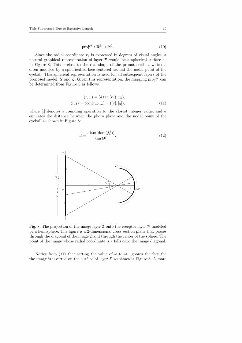
Since the radial coordinate ro is expressed in degrees of visual angles, anatural graphical representation of layer P would be a spherical surface asin Figure 8. This is close to the real shape of the primate retina, which isoften modeled by a spherical surface centered around the nodal point of theeyeball. This spherical representation is used for all subsequent layers of theproposed model: U and L. Given this representation, the mapping projpI canbe determined from Figure 8 as follows:

(r,ω) = (d tan (ro),ωo),

(i, j) = proj(ro,ωo) = ([x], [y]), (11)

where [.] denotes a rounding operation to the closest integer value, and demulates the distance between the photo plane and the nodal point of theeyeball as shown in Figure 8:

d =diam(dom(f I

k ))

tanΘI. (12)

ror

ΘI

Θp

diam

(dom

(fI k)

d

I

P

Fig. 8: The projection of the image layer I onto the receptor layer P modeledby a hemisphere. The figure is a 2-dimensional cross section plane that passesthrough the diagonal of the image I and through the center of the sphere. Thepoint of the image whose radial coordinate is r falls onto the image diagonal.

Notice from (11) that setting the value of ω to ωo ignores the fact thethe image is inverted on the surface of layer P as shown is Figure 8. A more

20 Ala Aboudib et al.

faithful way would be to set ω to ωo+π. However, this inversion can be safelyignored since it has no significance on the visual processing task in question.

Also notice that in our experiments, we always consider that the center ofthe fovea is fixated at the image’s center as in Figure 10. However, this modeloffers the possibility to fixate the fovea at any arbitrary point of the image oreven outside its borders as shown in Figure 9, which is a useful property fordesigning models that needs to emulate saccadic eye movements.

(a) (b)

Fig. 9: The acquisition of the signal of layer P is totally independent of thesize, position and the resolution of the image I. In (a), the visual angle of theimage is set to ΘI = 10◦, but the fovea falls onto the upper-left corner of theimage so that a part of the image falls outside of the visual field of layer P. In(b), the fovea center falls outside of the image borders, the value of ΘI is setto 4◦.

The input signal to the point fpk (ro,ωo) is then defined as:

sIpk (fpk (ro,ωo)) = {f I

k�(i, j)|(i, j) ∈ RFIp

k (fpk (ro,ωo)),

k = k�,

and f Ik�(i, j) ∈ I}, (13)

and finally, sampling is applied by computing the value of each point fpk (ro,ωo)

as follows:

fpk (ro,ωo) = φIp

k (sIpk (fpk (ro,ωo))), (14)

Title Suppressed Due to Excessive Length 21

where φIp is a mapping defined on a given set A as follows:

∀A,φIpk (A) =

�A ifA �= φ.0 Otherwise,

(15)

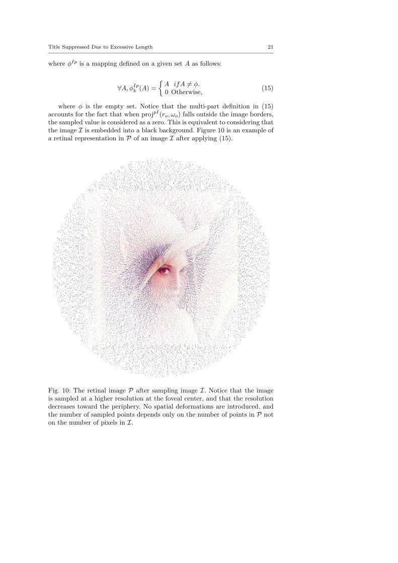
where φ is the empty set. Notice that the multi-part definition in (15)accounts for the fact that when projpI(ro,ωo) falls outside the image borders,the sampled value is considered as a zero. This is equivalent to considering thatthe image I is embedded into a black background. Figure 10 is an example ofa retinal representation in P of an image I after applying (15).

Fig. 10: The retinal image P after sampling image I. Notice that the imageis sampled at a higher resolution at the foveal center, and that the resolutiondecreases toward the periphery. No spatial deformations are introduced, andthe number of sampled points depends only on the number of points in P noton the number of pixels in I.

22 Ala Aboudib et al.

5.3 The feature map layer U

The next layer, is the feature map layer U . This layer is composed of 9 featuremaps representing intensity contrast, color opponency and local orientationselectivity, which are the basic three feature dimensions originally used in (Ittiet al, 1998):

U(Θu,ψu,Du) = {fuk |fu

k : R2 → R,

σ(diam(dom(fuk ))) = Θu,

k ∈ {1, ...,Ku = 9}}. (16)

All points in U that have the same value for k form a single featuremap. The 9 feature maps emerging from the above definition, {fu

k=1}, {fuk=2},

{fuk=3},{fu

k=4}, {fuk=5}, {fu

k=6}, {fuk=7}, {fu

k=8} and {fuk=9}, are chosen to

represent intensity contrast, local orientations for 0◦, 45◦, 90◦, 135◦ and coloropponency for red-green, green-red, blue-yellow, yellow-blue, respectively. Thedistribution Du is chosen to be a circular grid as shown in Figure 12. Noticethat as in P, the density of points is higher in the fovea and decreases towardsthe periphery. Also notice that point coordinates in dom(fu

k ) are expressed inthe same units as coordinates in dom(fp

k ), and they belong to the same space.Each point fu

k in U has its own receptive field in the receptor layer Pspanning a set of coordinates in dom(fp

k ). Each such RF is defined as follows:

RFpuk (fu

k (ro,ωo)) = {(r,ω)|(r,ω) ∈ dom(fpk�),

(ro,ωo) ∈ dom(fuk ),

and �(x, y), (xo, yo)� ≤ ρ(ro,ωo)}, (17)

where �., .� is the euclidean distance operator, ρ(ro,ωo) is the eccentricity-dependent radius of a circle centered at (ro,ωo), and is given by:

ρ(ro,ωo) =

�αro if ro ≥ ψu

2 .

αψu

2 otherwise,(18)

where α is the slope associated with the cortical magnification factor (CMF).Notice that (18) reflects the fact that receptive fields of cells within the foveaof a given layer tend to have roughly equal radii. However, these radii begin toincrease linearly at the extremities of the fovea toward the periphery, which isbehind the cortical magnification effect observed in the primate visual system(Gattass et al, 1981, 1988; Isik et al, 2011).

Notice that a radius ρ(ro,ωo) is measured in degrees of visual angles. Thus,a more precise way to compute the distance between (x, y) and (xo, yo) in (17)is to use the great circle distance according to a spherical geometry defined onlayer U . However, the spherical surface model of layers P, U and L is supposed

Title Suppressed Due to Excessive Length 23

to be locally plane for simplicity, which allows for computing distances as beinglocally euclidean.

It is worth pointing out that the distribution Du can only be determinedif the number, sizes and positions of all receptive fields RFpu

k are known. Inother words, this distribution is chosen so that a certain overlap is respectedbetween these RFs; the overlap along the radial line pr, and the overlap pcbetween RFs on the same circle. Figure 11 shows and example configuration ofreceptive fields RFpu

k (fuk ) with overlaps pr = pc = 0.5, and Figure 12 depicts

its corresponding distribution Du.

Fig. 11: Receptive fields RFpuk associated with points in layer U . Notice that

these RFs are smaller and more dense in the fovea and grow bigger withdecreasing density toward the periphery emulating the cortical magnificationfactor. This configuration corresponds to circular and radial overlap valuespc = pr = 0.5, a visual angle span of Θu = 10◦ and a slope α = 0.16 for thecortical magnification factor.

24 Ala Aboudib et al.

The input signals to points belonging to feature maps for intensity contrastand local orientations are given by:

spuk (fuk (ro,ωo))k∈{1,...,5} = {fp

k�(r,ω)|(r,ω) ∈ RFpu

k (fuk (ro,ωo)),

k� ∈ {1, 2,Kp = 3},and fp

k�(r,ω) ∈ P}. (19)

Input signals to points within the feature map for red-green opponency aredefined as:

spuk (fuk (ro,ωo))k=6 = {fp

k�(r,ω)|(r,ω) ∈ RFpu

k (fuk (ro,ωo)),

(k� = 1 ∧ �(x, y), (xo, yo)� ≤ (δc/2)∨(k� = 2 ∧ �(x, y), (xo, yo)� > (δc/2)),

and fpk�(r,ω) ∈ P}, (20)

where δc is the diameter of the central zone of RFpuk (fu

k (r�o,ω

�o)) that has a

center-surround configuration. We notice from (20) that red-green opponencyis applied in the same way as in chromatic ganglion cells that get their inputsignals from L (red) cones in the central zone of their receptive fields, and fromM (green) cones in the surround.

Similarly, input signals for green-red, blue-yellow, yellow-blue feature mapsare defined respectively as follows:

spuk (fuk (ro,ωo))k=7 = {fp

k�(r,ω)|(r,ω) ∈ RFpu

k (fuk (ro,ωo)),

(k� = 2 ∧ �(x, y), (xo, yo)� ≤ (δc/2))∨(k� = 1 ∧ �(x, y), (xo, yo)� > (δc/2)),

and fpk�(r,ω) ∈ P}, (21)

spuk (fuk (ro,ωo))k=8 = {fp

k�(r,ω)|(r,ω) ∈ RFpu

k (fuk (ro,ωo)),

(k� = 3 ∧ �(x, y), (xo, yo)� ≤ (δc/2))∨(k� ∈ {1, 2} ∧ �(x, y), (xo, yo)� > (δc/2)),

and fpk�(r,ω) ∈ P}, (22)

Title Suppressed Due to Excessive Length 25

Fig. 12: An example distribution Du for points in layer U corresponding tocircular and radial overlap values pc = pr = 0.5 between the receptive fieldsRFpu

k associated with each point. This value is chosen for the clarity of display.A value of 0.8 is used for the experiments. The visual angle span of the layer’sdiameter is σ(diam(dom(fu

k ))) = Θu = 10◦.

spuk (fuk (ro,ωo))k=9 = {fp

k�(r,ω)|(r,ω) ∈ RFpu

k (fuk (ro,ωo)),

(k� ∈ {1, 2} ∧ �(x, y), (xo, yo)� ≤ (δc/2))∨(k� = 3 ∧ �(x, y), (xo, yo)� > (δc/2)),

and fpk�(r,ω) ∈ P}. (23)

The value of each point fuk in the feature maps is then computed by ap-

plying a linear mapping φpuk .

26 Ala Aboudib et al.

fuk (ro,ωo) = φpu

k (spuk (fuk (ro,ωo))). (24)

This mapping consists in applying a DoG kernel on each input signal for theintensity contrast and color opponency feature maps, and a Gabor (GB) kernelin feature maps for local orientations. DoG kernels are classically used to modelthe center-surround configuration of RFs of parasol and midget ganglion cellsinvolved in chromatic and achromatic vision, while GB kernels are typicallyused to model orientation selective responses of neurons in V1, as mentionedin Section 3.

The DoG model proposed by Rodieck in (Rodieck, 1965) is used to computethe kernel coefficients associated with a point at a coordinate (r,ω).

DoG(ro,ωo, r,ω) =g1π

δ21. exp(−�(x, y), (xo, yo)�2

δ21)−

g2π

δ22. exp(−�(x, y), (xo, yo)�2

δ22), (25)

where (ro,ωo) is the RF center to which (r,ω) belongs, δ1 and δ2 are thestandard deviations of the central and the surround Gaussians of DoG kernels,g1 and g2 are two constants used to control the relative strengths of the twoGaussians.

Coefficients of Gabor kernels (Gabor, 1946) are similarly defined as follows:

GB(ro,ωo, r,ω) = exp(−X2 + Y 2γ2

2δ3). cos(

2π

λX), s.t. (26)

X = (x− xo) cos θ + (y − yo) sin θ and

Y = −(x− xo) sin θ + (y − yo) cos θ. (27)

Figure 13 depicts some examples of DoG and GB kernels we used. The map-ping φpu

k is finally applied as the sum of elements of an input signal weightedby their corresponding kernel coefficients:

φpuk (spuk (fu

k (ro,ωo)))k∈{1,6,7,8,9} =

=�

fp(r,ω)⊆spuk (fu

k (ro,ωo))

mean(fp(r,ω)).DoG(ro,ωo, r,ω), (28)

φpuk (spuk (fu

k (ro,ωo)))k∈{2,3,4,5} =

=�

fp(r,ω)⊆spuk (fu

k (ro,ωo))

mean(fp(r,ω)).GB(ro,ωo, r,ω), (29)

where fp(r,ω) here is the set of all points fpk�(r,ω) in spuk (fu

k (ro,ωo)) definedon the same coordinate (r,ω). Figure 14 is an example of some feature mapswe obtain by applying the above mappings.

Title Suppressed Due to Excessive Length 27

(a)

(b)

(c)

(d)

Fig. 13: Some examples of the Difference of Gaussians (DoG) and Gabor (GB)kernels used for the mapping φpu

k . Notice that kernels whose RFs are closer tothe fovea in (a) and (c) are smaller in size in and defined on more points thatRFs in the periphery, (b) and (d), which is due to the cortical magnificationfactor. This difference in size and density is inspired by biological reality in theretina. The gray background and the size of points in these figures is adjustedfor the clarity of display.

5.4 The saliency map layer L

Finally, layer L is used to compute the saliency map:

L(Θ�,ψ�,D�) = {f �k|f �

k : R2 → R,

σ(diam(dom(f �k))) = Θ�,

D� = Du,

and k ∈ {K� = 1}}, (30)

This saliency map has exactly the same distribution of point coordinatesas that of feature maps. The RF of each point in L at a coordinate (ro,ωo)spans only the point at the same location in U .

RFu�k (f �

k(ro,ωo)) = {(r,ω)|(r,ω) ∈ dom(fuk ),

(ro,ωo) ∈ dom(f �k),

and (r,ω) = (ro,ωo)}. (31)

Before point values in L could be computed, a modulation function mu asdefined in (2) is applied to U . This modulation is used to increase the contrastof the most salient regions in each feature map in a similar way the mapnormalization operator N (.) is applied in (Itti et al, 1998).

28 Ala Aboudib et al.

(a) Retinal image P (b) Feature map {fuk=1} ⊂ U .

(c) Feature map {fuk=6} ⊂ U . (d) Feature map {fu

k=5} ⊂ U .

Fig. 14: The retinal image represented by the receptors layer P (a) and somecorresponding feature maps held by layer U : intensity contrast feature map (b),red-green opponency feature map (c) and 135◦-orientation feature map (d).These feature maps correspond to circular and radial overlap values pc = pr =0.8, a visual angle span of ΘI = 10◦ and a slope α = 0.16 for the corticalmagnification factor.

U = mu(U) = {f uk |f u

k : R2 → [0, 1],

dom(f uk ) = dom(fu

k ),

k ∈ {1, ..., ku = 9}}. (32)

The steps for computing the value of the modulated points f uk are the

following:

Title Suppressed Due to Excessive Length 29

1. A half-wave rectification is first applied to feature maps to remove negativevalues.

f uk = max(0, fu

k ). (33)

2. The values within each feature map are scaled to the interval [0, 1].

f uk ←

f uk −min

k(f u

k )

maxk

(f uk )−min

k(f u

k ). (34)

3. A multiplicative factor βk is computed.

βk =

�max

k(f u

k )−meank

(f uk )

�2

. (35)

4. The multiplicative factor βk is then applied to each point of the featuremaps.

f uk ← βkf

uk (36)

The input signal to each point in the saliency map can now be defined onthe modulated feature maps:

su�k (f �k(ro,ωo)) = {f u

k�(r,ω)|(r,ω) ∈ RFu�

k (f �k(ro,ωo)),

f uk� ∈ U .}. (37)

Finally, the saliency map is computed using the mapping φu�k , which is the

mean of all modulated feature maps in U .

f �k(ro,ωo) = φu�

k (su�k (f �k(ro,ωo)))

= mean(su�k (f �k(ro,ωo))). (38)

5.5 Creating fixation maps

Fixation maps are created by an iterative processes consisting of a Winner-Take-All (WTA) step, which extracts the coordinates of the most salient pointin the saliency map followed by an Inhibition-of-Return (IOR) step, whichguarantees that previously fixated locations should no longer be visited insubsequent iterations. Here are the details of these two steps:

1. A fixation location (ro,ωo) is extracted from the saliency map L.

(ro,ωo) = argmax(r,w)

f �k. (39)

30 Ala Aboudib et al.

2. IOR is applied using a modulation function m�.

m�k(L) :

f �k(r,ω) ←

�f �k(r,ω) if �(x, y), (xo, yo)� > h0 otherwise,

(40)

where h is the radius of the inhibited zone in visual angles.3. the pixel indexes (i, j) in the image I corresponding to the fixation location

(ro,ωo) are then computed using (11).

Figure 15 depicts an example of a saliency map in layer L and the corre-sponding smoothed saliency map. A smoothed saliency map is one consistingin convoluting a gaussian kernel on the extracted fixation locations, in orderto produce a continuous gray-scale saliency map of the same size as the inputimage I.

In the next section, we provide a performance evaluation of the proposedattention model along with a comparison with some of the state-of-the-artmodels, and a discussion of the results.

6 Results and discussion

In order to validate the performance of the proposed model on estimatingbottom-up visual saliency, we ran the algorithm on the CAT2000 test datasetprovided by the MIT saliency benchmark. This dataset contains 2000 imagesfrom 20 different categories with a fixed size of 1920× 1080 pixels (Borji et al,2013a).

Before beginning the test on the above dataset, we performed a minoroptimization of the model parameters on the CAT2000 train dataset containing2000 images of the same 20 categories as in the CAT2000 test set (Borji et al,2013a).

Hence, we set the model parameters as follows: The visual angles ΘI =Θp = Θu = Θ� = 10◦, which represent the visual field available to the system.The diameter of the fovea of all layers ψI = ψp = ψu = ψ� = 1◦. The totalnumber of receptors in P is set to 123853 of which 30000 are within the fovea.This is equivalent to 41284 total RGB pixels of which 10000 are within thefovea, as shown in Figures 7 and 10. This means that retinal images used by thealgorithm has more than 50 times less pixels than the original images, whichrepresents a significant reduction of information. The overlap parameters prand pc between RFs of points in U are both set to 0.8. The slope α in (18)associated with the cortical magnification factor in layer U is set to 0.16 whichis close to its value in layer V 1 of the ventral stream found by Gattass in(Gattass et al, 1988). For each image, the 250 most salient fixations locationsare extracted by an iterative WTA and IOR process. The radius h of theinhibited zone at each IOR iteration is set to 0.05◦ of visual angles.

Title Suppressed Due to Excessive Length 31

(a)

(b) (c)

Fig. 15: An example of a saliency map carried by layer L (a) where the sizeof single points is adapted for a better clarity of display. The correspondingsmoothed saliency map is shown in (b) made by convoluting a Gaussian ker-nel on the first 250 fixation locations. In (c), the smoothed saliency map issuperimposed on the original image I.

Parameters of DoG kernels were adapted from (Rodieck, 1965). We setg2/g1 to 0.8, δ2/δ1 to 3 and ρ/δ1 to 11.8, where g2/g1 is a measure of theratio of strength of the surround to the center Gaussians of the DoG kernel,and δ1 and δ2 are the effective widths of the center and surround Gaussians,respectively.

For Gabor kernels, we adapted parameter values used for designing simplecells in the Hmax model (Serre et al, 2007); The aspect ratio is set as γ = 0.3.We also set δ3/λ = 0.8 and ρ/δ3 = 2.5, where δ3 is the effective width of theGaussian component of the filter, λ is the wavelength of the cosine component,

32 Ala Aboudib et al.

and ρ in both DoG and Gabor kernels denotes the eccentricity-dependentradius of a given kernel computed from (18) and expressed in visual angles.

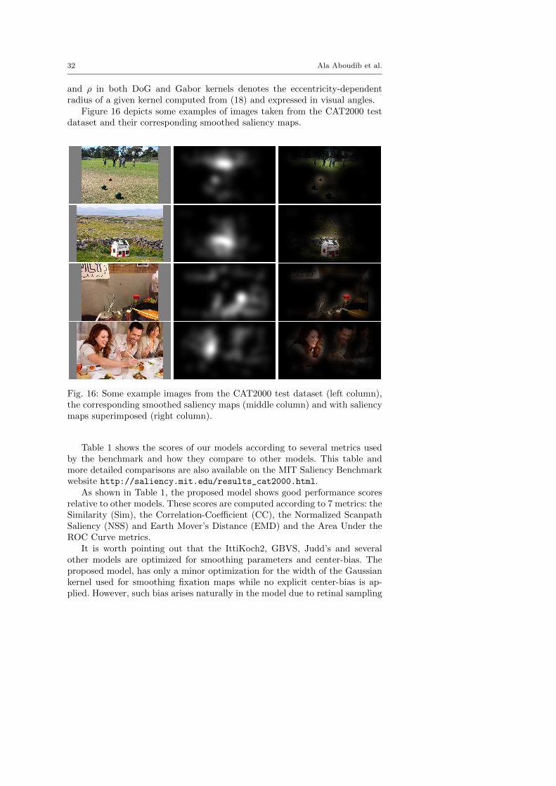
Figure 16 depicts some examples of images taken from the CAT2000 testdataset and their corresponding smoothed saliency maps.

Fig. 16: Some example images from the CAT2000 test dataset (left column),the corresponding smoothed saliency maps (middle column) and with saliencymaps superimposed (right column).

Table 1 shows the scores of our models according to several metrics usedby the benchmark and how they compare to other models. This table andmore detailed comparisons are also available on the MIT Saliency Benchmarkwebsite http://saliency.mit.edu/results_cat2000.html.

As shown in Table 1, the proposed model shows good performance scoresrelative to other models. These scores are computed according to 7 metrics: theSimilarity (Sim), the Correlation-Coefficient (CC), the Normalized ScanpathSaliency (NSS) and Earth Mover’s Distance (EMD) and the Area Under theROC Curve metrics.

It is worth pointing out that the IttiKoch2, GBVS, Judd’s and severalother models are optimized for smoothing parameters and center-bias. Theproposed model, has only a minor optimization for the width of the Gaussiankernel used for smoothing fixation maps while no explicit center-bias is ap-plied. However, such bias arises naturally in the model due to retinal sampling

Title Suppressed Due to Excessive Length 33

Model Sim AUC-Judd

EMD(Loweris bet-ter)

AUC-Borji

CC NSS sAUC

Proposedmodel

0.58 0.80 2.10 0.77 0.64 1.57 0.55

BMS Zhang and Sclaroff(2013)

0.61 0.85 1.95 0.84 0.67 1.67 0.59

GBVS Harel et al (2006) 0.51 0.80 2.99 0.79 0.50 1.23 0.58Context-Awaresaliency

Goferman et al (2012) 0.50 0.77 3.09 0.76 0.42 1.07 0.60

AWS Garcia-Diaz et al (2012) 0.49 0.76 3.36 0.75 0.42 1.09 0.62IttiKock2 0.48 0.77 3.44 0.76 0.42 1.06 0.59WMAP Lopez-Garcıa et al

(2011)0.47 0.75 3.28 0.69 0.38 1.01 0.60

Juddmodel

Judd et al (2009) 0.46 0.84 3.61 0.84 0.54 1.30 0.56

Torralbasaliency

Torralba et al (2006) 0.45 0.72 3.44 0.71 0.33 0.85 0.58

Murraymodel

Murray et al (2011) 0.43 0.70 3.79 0.70 0.30 0.77 0.59

SUNsaliency

Zhang et al (2008) 0.43 0.70 3.42 0.69 0.30 0.77 0.57

IttiKock Itti et al (1998) 0.34 0.56 4.66 0.53 0.09 0.25 0.52Achanta Achanta et al (2009) 0.33 0.57 4.45 0.55 0.11 0.29 0.52

Table 1: A performance comparison between the proposed model and othermodels on the CAT2000 test dataset of the MIT Saliency Benchmark. Theseresults can be found on the MIT saliency benchmark Web page http:

//saliency.mit.edu/results_cat2000.html.

and cortical magnification factors, which allocate more resources to processingcentral zones of the image than to peripheral ones. It would be interesting toexplore the role of retinal sampling and cortical magnification in influencingcenter-bias that human subjects manifest when free viewing images.

An important point to discuss is the fact the attentional behavior mani-fested by eye fixations differs as a function of the viewing distance, (or equiva-lently the visual angle) between the subject and an image (Borji et al, 2013b).However, attention models in Table 1 do not have a direct way for measuringtheir performance as a function of the visual angle. This makes interpretingthe performance of such models against a given saliency dataset more ambigu-ous and less straightforward. For example, suppose having two datasets D1

and D2, associated with two visual angles θ1 and θ2, respectively. If a givenattention model performs better on D1 than on D2, there would be no clearway for determining whether this is due to the fact that it is intrinsically moreadapted to the angle θ1 that to θ2, or due to other factors.

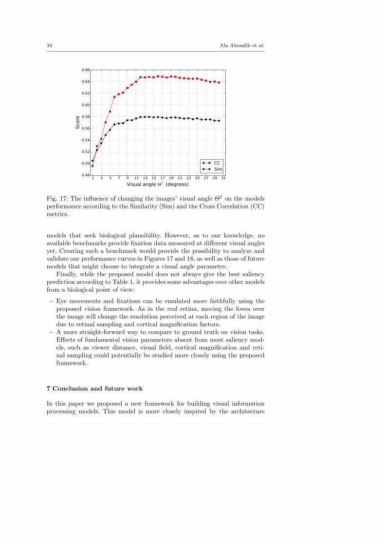
The model we propose provides the possibility to fix all other parameterswhile varying the image’s visual angle ΘI . Figures 17 and 18 depict how theperformance of the proposed attention algorithm varies according to differentevaluation metrics as a function of ΘI . This provides a mechanism to checkwhether the model matches ground truth attentional behavior when measuredat different visual angles. We think that this is a useful factor to consider for

34 Ala Aboudib et al.

� � � � � �� �� �� �� �� �� �� �� �� �� ��

�������������� ����������

����

����

����

����

����

����

����

����

����

����

�����

��

���

Fig. 17: The influence of changing the images’ visual angle ΘI on the modelsperformance according to the Similarity (Sim) and the Cross Correlation (CC)metrics.

models that seek biological plausibility. However, as to our knowledge, noavailable benchmarks provide fixation data measured at different visual anglesyet. Creating such a benchmark would provide the possibility to analyze andvalidate our performance curves in Figures 17 and 18, as well as those of futuremodels that might choose to integrate a visual angle parameter.

Finally, while the proposed model does not always give the best saliencyprediction according to Table 1, it provides some advantages over other modelsfrom a biological point of view:

– Eye movements and fixations can be emulated more faithfully using theproposed vision framework. As in the real retina, moving the fovea overthe image will change the resolution perceived at each region of the imagedue to retinal sampling and cortical magnification factors.

– A more straight-forward way to compare to ground truth on vision tasks.Effects of fundamental vision parameters absent from most saliency mod-els, such as viewer distance, visual field, cortical magnification and reti-nal sampling could potentially be studied more closely using the proposedframework.

7 Conclusion and future work

In this paper we proposed a new framework for building visual informationprocessing models. This model is more closely inspired by the architecture

Title Suppressed Due to Excessive Length 35

� � � � � �� �� �� �� �� �� �� �� �� �� ��

�������������� ����������

���

���

���

���

���

���

���

���������

���

Fig. 18: The influence of changing the images’ visual angle ΘI on the modelsperformance according to the Normalized Scanpath Saliency (NSS) metric.

of the primate visual system, and is motivated by the recent trend in thecomputer vision community toward a closer modeling of the visual system inthe hope of going beyond some limitations in current vision systems.

We have seen that the architecture of the proposed framework offers someinteresting properties found in the visual system. For example, the presence ofa receptor layer makes the acquired image signal totally independent from theinput image’s resolution and size. It also motivates the use of such a frameworkfor applications such like saccadic eye movements since the receptor layer isnot constrained by the image borders and can be used to receive its signal fromany part of the input scene. Moreover, the proposed framework has a very clearnotion of a visual angle emulating the ubiquitous presence of this parameter inbiological vision. This provides the possibility to better understand the influ-ence of a viewer’s distance from an image on vision tasks. Another importantproperty the framework offers is the information reduction by means of retinalsampling and cortical magnification which are two important and omnipresentfactors of primate visual systems. We have seen that these two mechanismscan be implemented seamlessly, while avoiding classical problems like spatialdeformations and the dependency on the input image size.

In Section 5, we proposed a saliency-driven model of attention built ontop of the proposed vision framework. We showed that this model attainsstate-of-the-art performance. More particularly, we showed that it has a bet-ter performance than Itti and Koch’s model on which it is based, while usinglower resolution and a fewer number of feature maps. This application mo-tivated the use of the proposed vision framework and raises some important

36 Ala Aboudib et al.

questions such as the role of the visual angle in attention modeling and its im-portance for a better understanding of attentional behavior and benchmarkingresults. One possible method we propose to start such exploration, would beto design an attention benchmark that provide eye-fixation data on a givendataset for a range of visual angles. It would be then interesting to study howmodels’ performances should be analyzed and understood given this variabilityof fixation data associated with different visual angles.

In future work, we will also consider the question of how common architec-tures for visual processing, especially Convolutional Neural Networks (CNNs)might be adapted for being implemented using the proposed framework. Thechallenge would be in modifying its learning algorithm so that it can takethe cortical magnification factor into account and the associated variability inkernel sizes in each layer.

Another research perspective would be to use the proposed framework forimplementing attention-based object recognition processors to account for theretinal transformation stage in models such like (Zheng et al, 2015).

The proposed framework and the associated attention model are alreadyimplemented and are publicly available as a Git repository on the Web1. How-ever, future work will include further development and improvement of the pro-posed framework along with its code implementation. We hope that throughcollaboration, this framework could evolve as an alternative, full-fledged tool-box for neuro-inspired visual processing, in the same way as current program-ming libraries offer optimized implementations of traditional image processingalgorithms.

8 Compliance with Ethical Standards

This study was funded by the European Research Council under the Euro-pean Union’s Seventh Framework Program (FP7/2007-2013) / ERC grantagreement n◦ 290901. This article does not contain any studies with humanparticipants or animals performed by any of the authors.

References

Aboudib A, Gripon V, Coppin G (2015) A model of bottom-up visual attentionusing cortical magnification. In: Acoustics, Speech and Signal Processing(ICASSP), 2015 IEEE International Conference on, pp 1493–1497, DOI10.1109/ICASSP.2015.7178219

Achanta R, Hemami S, Estrada F, Susstrunk S (2009) Frequency-tuned salientregion detection. In: IEEE Conference on Computer Vision and PatternRecognition (CVPR), 2009, IEEE, pp 1597–1604

Anselmi F, Rosasco L, Poggio T (2015) On invariance and selectivity in rep-resentation learning. arXiv preprint arXiv:150305938

1 https://bitbucket.org/ala aboudib/see

Title Suppressed Due to Excessive Length 37

Bonaiuto J, Itti L (2005) Combining attention and recognition for rapid sceneanalysis. In: Computer Vision and Pattern Recognition-Workshops, 2005.CVPR Workshops. IEEE Computer Society Conference on, IEEE, pp 90–90

Borji A, Itti L (2013) State-of-the-art in visual attention modeling. PatternAnalysis and Machine Intelligence, IEEE Transactions on 35(1):185–207

Borji A, Sihite DN, Itti L (2013a) Quantitative analysis of human-model agree-ment in visual saliency modeling: A comparative study. Image Processing,IEEE Transactions on 22(1):55–69

Borji A, Tavakoli HR, Sihite DN, Itti L (2013b) Analysis of scores, datasets,and models in visual saliency prediction. In: Computer Vision (ICCV), 2013IEEE International Conference on, IEEE, pp 921–928

Borji A, Sihite DN, Itti L (2014) What/where to look next? modeling top-down visual attention in complex interactive environments. Systems, Man,and Cybernetics: Systems, IEEE Transactions on 44(5):523–538

Dowling JE (1987) The retina: an approachable part of the brain. HarvardUniversity Press

Freeman J, Simoncelli EP (2011) Metamers of the ventral stream. Natureneuroscience 14(9):1195–1201

Gabor D (1946) Theory of communication. part 1: The analysis of informa-tion. Journal of the Institution of Electrical Engineers-Part III: Radio andCommunication Engineering 93(26):429–441

Gao F, Zhang Y, Wang J, Sun J, Yang E, Hussain A (2015) Visual attentionmodel based vehicle target detection in synthetic aperture radar images: Anovel approach. Cognitive Computation 7(4):434–444

Garcia-Diaz A, Leboran V, Fdez-Vidal XR, Pardo XM (2012) On the rela-tionship between optical variability, visual saliency, and eye fixations: Acomputational approach. Journal of vision 12(6):17–17

Gattass R, Gross C, Sandell J (1981) Visual topography of v2 in the macaque.Journal of Comparative Neurology 201(4):519–539

Gattass R, Sousa A, Gross C (1988) Visuotopic organization and extent of v3and v4 of the macaque. The Journal of neuroscience 8(6):1831–1845

Goferman S, Zelnik-Manor L, Tal A (2012) Context-aware saliency detec-tion. IEEE Transactions on Pattern Analysis and Machine Intelligence34(10):1915–1926

Gonzalez RC, Woods RE (2002) Digital image processingGoodale MA, Milner AD (1992) Separate visual pathways for perception andaction. Trends in neurosciences 15(1):20–25

Harel J, Koch C, Perona P (2006) Graph-based visual saliency. In: Advancesin neural information processing systems, pp 545–552

Hubel DH, Wiesel TN (1959) Receptive fields of single neurones in the cat’sstriate cortex. The Journal of physiology 148(3):574–591

Hubel DH, Wiesel TN (1962) Receptive fields, binocular interaction and func-tional architecture in the cat’s visual cortex. The Journal of physiology160(1):106–154

Isik L, Leibo JZ, Mutch J, Lee SW, Poggio T (2011) A hierarchical model ofperipheral vision. Tech. rep., MIT’s Computer Science and Artificial Intel-

38 Ala Aboudib et al.

ligence LaboratoryItti L, Koch C, Niebur E (1998) A model of saliency-based visual attention forrapid scene analysis. IEEE Transactions on pattern analysis and machineintelligence 20(11):1254–1259

Judd T, Ehinger K, Durand F, Torralba A (2009) Learning to predict wherehumans look. In: IEEE Conference on Computer Vision and Pattern Recog-nition (CVPR), 2009, IEEE, pp 2106–2113

Koch C, Ullman S (1987) Shifts in selective visual attention: towards theunderlying neural circuitry. In: Matters of intelligence, Springer, pp 115–141

Krizhevsky A, Sutskever I, Hinton GE (2012) Imagenet classification with deepconvolutional neural networks. In: Advances in neural information process-ing systems, pp 1097–1105

Kruthiventi SS, Ayush K, Babu RV (2015) Deepfix: A fully convolutionalneural network for predicting human eye fixations. CoRR abs/1510.02927

Lake BM, Salakhutdinov R, Tenenbaum JB (2015) Human-level concept learn-ing through probabilistic program induction. Science 350(6266):1332–1338

Larochelle H, Hinton GE (2010) Learning to combine foveal glimpses with athird-order boltzmann machine. In: Lafferty J, Williams C, Shawe-TaylorJ, Zemel R, Culotta A (eds) Advances in Neural Information ProcessingSystems 23, Curran Associates, Inc., pp 1243–1251

LeCun Y, Bottou L, Bengio Y, Haffner P (1998) Gradient-based learning ap-plied to document recognition. Proceedings of the IEEE 86(11):2278–2324

Lee H, Battle A, Raina R, Ng AY (2006) Efficient sparse coding algorithms.In: Advances in neural information processing systems, pp 801–808

Liu H, Liu Y, Sun F (2015) Robust exemplar extraction using structuredsparse coding. IEEE transactions on neural networks and learning systems26(8):1816–1821

Lopez-Garcıa F, Dosil R, Pardo XM, Fdez-Vidal XR (2011) Scene recognitionthrough visual attention and image features: A comparison between sift andsurf approaches. INTECH Open Access Publisher

Marcelja S (1980) Mathematical description of the responses of simple corticalcells*. JOSA 70(11):1297–1300

Marr D (1982) Vision, a computational investigation into the human repre-sentation and processing of visual information. WH San Francisco: Freemanand Company

Martınez J, Robles LA (2006) A new foveal cartesian geometry approach usedfor object tracking. SPPRA 6:133–139

McCulloch WS, Pitts W (1943) A logical calculus of the ideas immanent innervous activity. The bulletin of mathematical biophysics 5(4):115–133

Milner AD, Goodale MA (2008) Two visual systems re-viewed. Neuropsycholo-gia 46(3):774–785

Murray N, Vanrell M, Otazu X, Parraga CA (2011) Saliency estimation usinga non-parametric low-level vision model. In: IEEE Conference on ComputerVision and Pattern Recognition (CVPR), 2011, IEEE, pp 433–440

Title Suppressed Due to Excessive Length 39

Pan J, Li X, Li X, Pang Y (2016) Incrementally detecting moving objects invideo with sparsity and connectivity. Cognitive Computation 8(3):420–428

Poggio T, Mutch J, Isik L (2014) Computational role of eccentricity dependentcortical magnification. arXiv preprint arXiv:14061770

Ranzato M, Hinton G, LeCun Y (2015) Guest editorial: Deep learning. Inter-national Journal of Computer Vision 113(1):1–2, DOI 10.1007/s11263-015-0813-1

Ray S, Scott S, Blockeel H (2010) Encyclopedia of Machine Learning,Springer US, Boston, MA, chap Multi-Instance Learning, pp 701–710. DOI10.1007/978-0-387-30164-8 569, URL http://dx.doi.org/10.1007/978-

0-387-30164-8_569

Rodieck RW (1965) Quantitative analysis of cat retinal ganglion cell responseto visual stimuli. Vision research 5(12):583–601

Rybak IA, Gusakova V, Golovan A, Podladchikova L, Shevtsova N (1998) Amodel of attention-guided visual perception and recognition. Vision research38(15):2387–2400

Salin PA, Bullier J (1995) Corticocortical connections in the visual system:structure and function. Physiological reviews 75(1):107–155

Schwartz EL (1984) Anatomical and physiological correlates of visual compu-tation from striate to infero-temporal cortex. Systems, Man and Cybernet-ics, IEEE Transactions on (2):257–271

Serre T, Wolf L, Bileschi S, Riesenhuber M, Poggio T (2007) Robust objectrecognition with cortex-like mechanisms. Pattern Analysis and Machine In-telligence, IEEE Transactions on 29(3):411–426

Torralba A, Oliva A, Castelhano MS, Henderson JM (2006) Contextual guid-ance of eye movements and attention in real-world scenes: the role of globalfeatures in object search. Psychological review 113(4):766

Treisman AM, Gelade G (1980) A feature-integration theory of attention. Cog-nitive psychology 12(1):97–136

Tu Z, Abel A, Zhang L, Luo B, Hussain A (2016) A new spatio-temporalsaliency-based video object segmentation. Cognitive Computation pp 1–19

Walther D, Koch C (2007) Attention in hierarchical models of object recogni-tion. Progress in brain research 165:57–78

Walther D, Rutishauser U, Koch C, Perona P (2004) On the usefulness of at-tention for object recognition. In: Workshop on Attention and Performancein Computational Vision at ECCV, Citeseer, pp 96–103

Wohrer A, Kornprobst P (2009) Virtual retina: a biological retina model andsimulator, with contrast gain control. Journal of computational neuroscience26(2):219–249

Zhang J, Sclaroff S (2013) Saliency detection: A boolean map approach. In:Proceedings of the IEEE International Conference on Computer Vision, pp153–160

Zhang L, Tong MH, Marks TK, Shan H, Cottrell GW (2008) Sun: A bayesianframework for saliency using natural statistics. Journal of vision 8(7):32

Zhao J, Sun S, Liu X, Sun J, Yang A (2014) A novel biologically inspiredvisual saliency model. Cognitive Computation 6(4):841–848

40 Ala Aboudib et al.

Zheng Y, Zemel R, Zhang YJ, Larochelle H (2015) A neural autoregressiveapproach to attention-based recognition. International Journal of ComputerVision 113(1):67–79

Zhu JY, Wu J, Xu Y, Chang E, Tu Z (2015) Unsupervised object class discov-ery via saliency-guided multiple class learning. Pattern Analysis and Ma-chine Intelligence, IEEE Transactions on 37(4):862–875

View publication statsView publication stats