a biologically inspired method for vision-based docking of

Robotics and Autonomous Systems 55 (2007) 769–784www.elsevier.com/locate/robot

A biologically inspired method for vision-based docking ofwheeled mobile robots

Emily M.P. Lowa,∗, Ian R. Manchesterb, Andrey V. Savkina

a School of Electrical Engineering and Telecommunications, University of New South Wales, Sydney 2052, Australiab Department of Applied Physics and Electronics, Umea University, SE-901 87 Umea, Sweden

Received 20 February 2006; accepted 6 April 2007Available online 17 May 2007

Abstract

We present a new control law for the problem of docking a wheeled robot to a target at a certain location with a desired heading. Recentresearch into insect navigation has inspired a solution which uses only one video camera. The control law is of the “behavioral” type in that allcontrol actions are based on immediate visual information. Docking success under certain conditions is proved mathematically and simulationstudies show the control law to be robust to camera intrinsic parameter errors. Experiments were performed for verification of the control law.c 2007 Elsevier B.V. All rights reserved.

Keywords: Wheeled robots; Navigation; Robust control; Computer vision

1. Introduction

It is currently very popular among roboticists to drawinspiration from the animal kingdom [1,2]. This trend is termed“biomimetics”. Robot navigation strategies thus derived, oftencategorized as “behavioral” or “reactive” robotics, aim at theconstruction of simple control strategies which use directsensory information, rather than a structured environmentalmodel. Such strategies demonstrate an intimate relationshipbetween movement control and vision. The use of visionis recommended when robots must operate in a dynamicenvironment.

In this paper we present one such control strategy andits experimentation for the problem of positioning a wheeledrobot to a target at a certain location with a certain heading,i.e. docking, using information provided by a video camera.The kinematics of the robot are non-holonomic, so standardtechniques of visual servoing (see, e.g., [3]) cannot be directlyapplied. We introduce a change of variables and a camera space

This work was supported by the Australian Research Council.∗ Corresponding author. Tel.: +61 2 9385 5701; fax: +61 2 9385 5993.

E-mail addresses: [email protected] (E.M.P. Low),[email protected] (I.R. Manchester), [email protected](A.V. Savkin).

regulation condition which allow solution of the problem via arelatively simple nonlinear control law.

This paper draws on previous work in precision missileguidance [4,5] that involved missile guidance with an impact-angle constraint, and was built on a combination of geometricalconsiderations, and recent work in robust control and filteringtheory [6–10].

The remarkable ability of honeybees and other insects likethem to navigate effectively using very little information is asource of inspiration for the proposed control strategy. In par-ticular, the work of Srinivasan and his co-authors [11–13], ex-plaining the use of optical-flow in honeybee navigation wherea honeybee makes a smooth landing on a surface without theknowledge of its vertical height above the surface. Analogousto this, the control strategy we present, which is originally pub-lished by the co-authors [14], is solely based on instantaneouslyavailable visual information and requires no information on thedistance to the target. Thus, it is particularly suitable for robotsequipped with a video camera as their primary sensor.

From a behavioral point of view, the problem of controllingeye–head systems is a fundamental issue for completionof specific tasks [15]. In this paper, we describe andexperimentally investigate a vision-based docking system [16]for controlling a wheeled mobile robot approach to a statictarget using a video camera. The docking system consists of

0921-8890/$ - see front matter c 2007 Elsevier B.V. All rights reserved.doi:10.1016/j.robot.2007.04.002

http://www.elsevier.com/locate/robot

mailto:[email protected]



http://dx.doi.org/10.1016/j.robot.2007.04.002

770 E.M.P. Low et al. / Robotics and Autonomous Systems 55 (2007) 769–784

the behavior-based control law and a vision design. The visiondesign includes a pan video camera with a visual gaze algorithmthat mimics the ability of many living insects to control theirdirection of gaze, enabling fixation on a specific part of anenvironment. As a result, it captures images more suitable forcompletion of a task.

Computer vision-processing techniques [17] allow wheeledrobots to understand an environment. Underlying all thesetechniques is the need to recognize an object of interestin an environment. We use both edge and region detectiontechniques. Specifically, intersection of the edges of a rectangleproduces corners and region information is employed in theform of optical flow. Subsequently, these visual parameters areprovided to the control law which regulates the motion of thewheeled robot to the target.

The proposed vision-based robotic docking system wasimplemented and verified by various experiments using awheeled robot and a pan video camera in a laboratory setting.In each experiment, the aim was to dock a wheeled robot ata certain location with a different heading. The experimentalresults demonstrated the effectiveness of the control law.

Docking is required in almost all applications of wheeledrobots particularly when mobile wheeled robots are required torecharge their batteries for long term operation. It is envisagedthat wheeled robots will play a significant role in search andrescue operations, in port automation and even in autonomoushighway systems.

The rest of the paper is organized as follows. Section 2 dis-cusses work in the literature related to the docking problem.Section 3 defines the problem statement. Section 4 introducesthe control law for docking a wheeled mobile robot and presentsthe derivation and mathematically rigorous analysis of the con-trol law. Section 5 includes simulation studies on the robust-ness of the control law. Section 6 describes the design of thevision-based docking system and reports experimental results.Our conclusions are drawn in Section 7. Lastly, an appendixincludes computer vision algorithms used in this work.

2. Related work

Most studies of this problem can be roughly grouped intotwo approaches. One focuses on the robot’s “configurationspace”, i.e. the relative positions and angles of the robot andtarget, and perhaps obstacles, in the plane. All these relationsare assumed to be available to the control law, and from themit chooses some desirable path. Examples are found in [18–21]and references therein.

The method described in [18] is similar in its approachto the method presented in this paper, in that the aim is tofollow to a circular path. The main differences are that, firstly,they assume a slightly simpler kinematic model (often termedthe unicycle model), and secondly, they are able to proveexponential stabilization to the desired final location, but atthe expense of a control law which is more complicated andrequires more information.

The other main approach focuses on “camera space” or“visual space”. It is no longer assumed that the robot has access

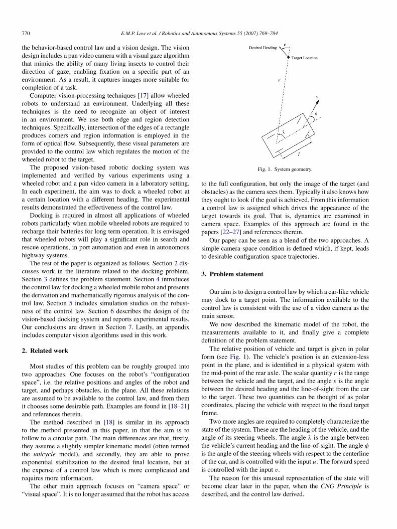
Fig. 1. System geometry.

to the full configuration, but only the image of the target (andobstacles) as the camera sees them. Typically it also knows howthey ought to look if the goal is achieved. From this informationa control law is assigned which drives the appearance of thetarget towards its goal. That is, dynamics are examined incamera space. Examples of this approach are found in thepapers [22–27] and references therein.

Our paper can be seen as a blend of the two approaches. Asimple camera-space condition is defined which, if kept, leadsto desirable configuration-space trajectories.

3. Problem statement

Our aim is to design a control law by which a car-like vehiclemay dock to a target point. The information available to thecontrol law is consistent with the use of a video camera as themain sensor.

We now described the kinematic model of the robot, themeasurements available to it, and finally give a completedefinition of the problem statement.

The relative position of vehicle and target is given in polarform (see Fig. 1). The vehicle’s position is an extension-lesspoint in the plane, and is identified in a physical system withthe mid-point of the rear axle. The scalar quantity r is the rangebetween the vehicle and the target, and the angle ε is the anglebetween the desired heading and the line-of-sight from the carto the target. These two quantities can be thought of as polarcoordinates, placing the vehicle with respect to the fixed targetframe.

Two more angles are required to completely characterize thestate of the system. These are the heading of the vehicle, and theangle of its steering wheels. The angle λ is the angle betweenthe vehicle’s current heading and the line-of-sight. The angle φ

is the angle of the steering wheels with respect to the centerlineof the car, and is controlled with the input u. The forward speedis controlled with the input v.

The reason for this unusual representation of the state willbecome clear later in the paper, when the CNG Principle isdescribed, and the control law derived.

E.M.P. Low et al. / Robotics and Autonomous Systems 55 (2007) 769–784 771

The state-space of the car–target system is then the manifoldR × T3 of states (r, λ, ε, φ), where T is the circle group:R mod 2πZ. The equations of motion on this manifoldare given by the following differential equations. These aregiven for a front-wheel-drive car. To make our control lawindependent of the forward-velocity of the car, the dynamicsare derived with respect to path length, not time.

The change of variables ds = v cos φdt allows us to passfrom one representation to another.

Hereafter, x denotes derivative of a variable x with respectto path length s. The dynamics of the states in this form aregiven below:

λ = sin λ

r− tan φ

l, ε = − sin λ

r, (1)

r = − cos λ, φ = uv cos φ

. (2)

Where l is the distance between the front wheels and rearwheels.

We now discuss the measurements available. Inspired by theelegant instinctual behavior of insects, and the practical need forcontrolling vehicles with simple sensors, we use a measurementmodel consistent with a single video camera mounted on therobot, and an optical flow algorithm.

The main restriction felt with this model is that the rangeto the the target, r , is not directly measurable. Furthermore, incertain situations it is unobservable, or weakly observable, fromthe measurements we do have. For this reason we do not use thisquantity in our control law.

The angular position of the dock-target in the field of view isthe angle λ. The derivative of this variable is the optical flow ofthe image. An optical flow algorithm such as [28] can calculatethis value.

The angle ε must be known, as it is not an environmentalvariable, but part of the problem statement. This variable iscalculated by assuming the target-heading is defined as anabstract bearing, the heading of the vehicle is dead-reckonedand from this and the angle λ, ε is calculated. Details areprovided later in the paper.

Further to the information from the video camera, we needsome knowledge of the internal state of the vehicle. Specifi-cally, we assume knowledge of the forward speed v, the angleof the steering wheels φ and the distance between the axles l.

3.1. Complete problem statement

Our complete problem statement is this. To find a controllaw of the form

u = f (l, φ, v, ε, λ, λ) (3)

such that range and angle error at final time, i.e. r(T ) and ε(T ),are minimized. Corresponding to this, we make the followingdefinition:

Definition 1. A docking manoeuvre is considered perfect ifthere exists some finite time T such that

r(T ) = 0,

limt→T

ε(t) = 0.

A limit is used in the above definition because if r = 0 the angleε is undefined.

4. Control law

From the optical flow measurements, we can cancel thecomponent due to the robot’s rotation (= v sin φ/ l), and retainonly the component due to the relative motion of robot anddock-target. We denote this remaining flow O f , so:

O f := λ + v sin φ

l. (4)

The control input u is then chosen as:

eh := λ − ε, ec := 2O f

v cos φ− tan φ

l, (5)

u := lv cos3 φ(aec + beh). (6)

Here we can think of eh as the heading error, and ec as thecurvature error, as the car describes a path toward the target.

The gains a and b should both be positive, and can be chosenwith the following guidelines:

• The dynamics of the linear system eh +ae

h +beh = 0 shouldrepresent suitable regulation to the desired path,

• The range r0 := 2/a should be small enough that divergencefrom the desired path within this region of the target isacceptable.

A discussion of the reasoning behind this control law, andthe tuning guidelines, is presented over the next two sections.

4.1. Control law derivation

The method with which we arrived at the above control lawis slightly different from most previous approaches. The controlobjective is to reach some final state, but rather than trying toderive a controller which provides some type of stability to thisstate, our approach has two stages.

Firstly, simple geometry allows us to pass from the terminalcondition to a condition on the instantaneous configuration ofthe vehicle, this is what we call the CNG Principle. Secondly,from this instantaneous condition we derive a feedback-controllaw using methods similar to feedback linearization.

The following theorem forms the basis of our control law,and was proved in [4]:

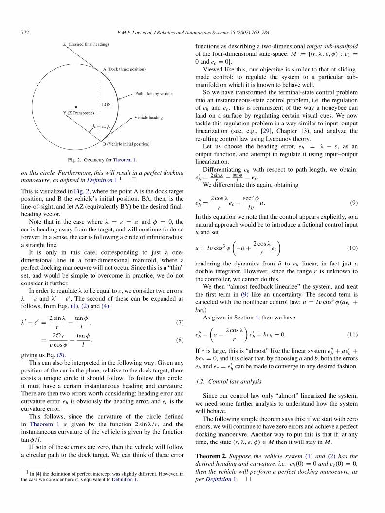
Theorem 1 (Circular-Navigation-Guidance Principle). Intro-duce the circle uniquely defined by the following properties:The initial and final positions of the vehicle lies on the circle;the desired final-heading vector at the target’s position is a tan-gent to the circle.

Suppose that a controller of the form (3) is designed suchthat the angles λ and ε are kept exactly equal over the fulldocking manoeuvre, then the vehicle’s trajectory will be an arc


Fig. 2. Geometry for Theorem 1.

on this circle. Furthermore, this will result in a perfect dockingmanoeuvre, as defined in Definition 1.1 This is visualized in Fig. 2, where the point A is the dock targetposition, and B the vehicle’s initial position. BA, then, is theline-of-sight, and let AZ (equivalently BY) be the desired final-heading vector.

Note that in the case where λ = ε = π and φ = 0, thecar is heading away from the target, and will continue to do soforever. In a sense, the car is following a circle of infinite radius:a straight line.

It is only in this case, corresponding to just a one-dimensional line in a four-dimensional manifold, where aperfect docking manoeuvre will not occur. Since this is a “thin”set, and would be simple to overcome in practice, we do notconsider it further.

In order to regulate λ to be equal to ε, we consider two errors:λ − ε and λ − ε. The second of these can be expanded asfollows, from Eqs. (1), (2) and (4):

λ − ε = 2 sin λ

r− tan φ

l, (7)

= 2O f

v cos φ− tan φ

l, (8)

giving us Eq. (5).This can also be interpreted in the following way: Given any

position of the car in the plane, relative to the dock target, thereexists a unique circle it should follow. To follow this circle,it must have a certain instantaneous heading and curvature.There are then two errors worth considering: heading error andcurvature error. eh is obviously the heading error, and ec is thecurvature error.

This follows, since the curvature of the circle definedin Theorem 1 is given by the function 2 sin λ/r , and theinstantaneous curvature of the vehicle is given by the functiontan φ/ l.

If both of these errors are zero, then the vehicle will followa circular path to the dock target. We can think of these error

1 In [4] the definition of perfect intercept was slightly different. However, inthe case we consider here it is equivalent to Definition 1.

functions as describing a two-dimensional target sub-manifoldof the four-dimensional state-space: M := (r, λ, ε, φ) : eh =0 and ec = 0.

Viewed like this, our objective is similar to that of sliding-mode control: to regulate the system to a particular sub-manifold on which it is known to behave well.

So we have transformed the terminal-state control probleminto an instantaneous-state control problem, i.e. the regulationof eh and ec. This is reminiscent of the way a honeybee canland on a surface by regulating certain visual cues. We nowtackle this regulation problem in a way similar to input–outputlinearization (see, e.g., [29], Chapter 13), and analyze theresulting control law using Lyapunov theory.

Let us choose the heading error, eh = λ − ε, as anoutput function, and attempt to regulate it using input–outputlinearization.

Differentiating eh with respect to path-length, we obtain:e

h = 2 sin λr − tan φ

l = ec.We differentiate this again, obtaining

eh = 2 cos λ

rec − sec3 φ

lvu. (9)

In this equation we note that the control appears explicitly, so anatural approach would be to introduce a fictional control inputu and set

u = lv cos3 φ

−u + 2 cos λ

rec

(10)

rendering the dynamics from u to eh linear, in fact just adouble integrator. However, since the range r is unknown tothe controller, we cannot do this.

We then “almost feedback linearize” the system, and treatthe first term in (9) like an uncertainty. The second term iscanceled with the nonlinear control law: u = lv cos3 φ(aec +beh)

As given in Section 4, then we have

eh +

a − 2 cos λ

r

e

h + beh = 0. (11)

If r is large, this is “almost” like the linear system eh + ae

h +beh = 0, and it is clear that, by choosing a and b, both the errorseh and ec = e

h can be made to converge in any desired fashion.

4.2. Control law analysis

Since our control law only “almost” linearized the system,we need some further analysis to understand how the systemwill behave.

The following simple theorem says this: if we start with zeroerrors, we will continue to have zero errors and achieve a perfectdocking manoeuvre. Another way to put this is that if, at anytime, the state (r, λ, ε, φ) ∈ M then it will stay in M .

Theorem 2. Suppose the vehicle system (1) and (2) has thedesired heading and curvature, i.e. eh(0) = 0 and ec(0) = 0,then the vehicle will perform a perfect docking manoeuvre, asper Definition 1.


Proof of Theorem 2. It is clear from the equation of the system(11) that, eh(t) = 0 and ec(t) = 0 at some time t , then theyhave been, and will be, zero for all time. This implies, then, thatλ = ε for all time, and the claim follows from Theorem 1.

Now suppose the state starts outside M , that is, withincorrect heading and curvature. Now we’d like to knowsomething about convergence to the target sub-manifold. Thedynamics of (11) are those of a linear system with time-varyingcoefficients, and can be analyzed with Lyapunov theory.

Theorem 3. Consider the function

V (eh, ec) := be2h + e2

c . (12)

This is a positive-definite quadratic form in the heading andcurvature errors, and may be considered as the distance to thetarget sub-manifold.

Let [s1, s2], s2 > s1 be any path interval over whichV (eh, ec, s) = 0 and the following inequality holds:

a − 2 cos λ/r > 0. (13)

Then V (eh(s2), ec(s2)) < V (eh(s1), ec(s1)). That is, over anyinterval of non-zero length, the norm of the errors strictlydecreases. Proof of Theorem 3. For the proof of this theorem, considerthe following linear parameter-varying realization of the system(11), with a state x = [ehec]T:

x = Ax + Bw (14)z = Cx . (15)

where

A =

0 1−b 2 cos λ/r − a

, B =

01

, C =

0 1

.

Furthermore, consider the Lyapunov function V (x) = xT Pxwhere

P =

b 00 1

. (16)

The derivative of this Lyapunov function with respect todistance travelled reduces to

V (x) = −2e2c (a − 2 cos λ/r). (17)

Now, for any s in the interval [s1, s2], it follows fromV (eh, ec, s) = 0 that x(s) = 0. Since x is observable fromec, it follows that s2

s1

ec(s)2ds > 0,

and since inequality (13) holds, clearly

δ := 2 s2

s1

ec(s)2

a − 2 cos λ(s)r(s)

ds > 0.

Now,

V (eh(s2), ec(s2)) = V (eh(s1), ec(s1))

+ s2

s1

V (eh, ec)ds,

= V (eh(s1), ec(s1)) − δ

< V (eh(s1), ec(s1)),

and the theorem is proved. This theorem reflects the following physically meaningful

problem: When the vehicle is very close to the desired targetlocation, large gains are required to make it swing around andtrack the correct path.

It should be noted that if the range is measurable, eitherthrough some other sensor device, or through vision-processingtechniques such as stereopsis, optical flow or image looming,this problem will still be present. Indeed, suppose the controllaw (10) were used, then as the range decreased the gains wouldbe come extremely large, due to the 1/r term. The actuatorconstraints on any real system would thus prevent the exactfeedback linearization which is attempted.

5. Robustness

It has been mentioned in the literature that a particularlyimportant test of a docking algorithm is the robustness of itsterminal positioning precision to imperfect modeling of thekinematics and camera calibration [27,19].

The parameters chosen for the simulation were: l = 1 m,v = 1 m/s, a = 4, b = 4.04. The initial conditions werer(0) = 7 m, λ(0) = π/4 rad, ε = π/4 rad, φ = π/8 rad.

These parameters imply that the area in which the path couldbegin to diverge is approximate 2/a = 0.5 m. Note that inall simulated cases, the terminal positioning error was muchsmaller than this.

In all the following simulations, the control law is derivedas above, as though all parameters were nominal. We thensimulate a system where parameters are perturbed by someamount.

5.1. Camera calibration

Here we simulate the effect of incorrect camera calibration.We skew the measurement of λ and the optical flow in a wayconsistent with an incorrect assumption on the focal length ofthe camera. We introduce the ratio k f as the true focal lengthdivided by the assumed focal length.

This parameter was varied from 0.6 to 1.8. In Fig. 3 wesee graphical plots of trajectories, and numerical data for thefinal range and final-angle error. It is clear that, althoughthe trajectories throughout the middle stage of the dockingmanoeuvre vary widely, in all cases the robot docked with lessthan 1 cm positioning error, and less than 10 angle error.

5.2. Control input gain

We now move on to consider errors in the kinematic model,specifically, in the steering wheel system. Firstly, we investigatewhat happens if the relationship between the control input andsteering-wheel movement is not what we expect. Instead ofthe assumed relation φ = u, we instead simulate the systemφ = kuu, where ku is an unknown gain term.


Fig. 3. The effect of incorrect camera calibration.

Fig. 4. The effect of incorrect u → φ gain.

Fig. 4 depicts the trajectories and error data as ku is variedfrom 0.2 to 5. It is noted that increasing ku significantly, whichmeans that our control input is stronger than we expect, haslittle effect on the performance of the vehicle. A larger effect isobserved when the control input is weaker than expected, butperformance is still very good.

Fig. 5. The effect of erroneous measurement of φ.

Reducing it significantly (to around 0.2) results in somelarge oscillations in the trajectory, and errors in both finalposition and final angle. However, reduction of ku even to 0.5,meaning our control input is half as strong as we think, does notsignificantly degrade performance.

5.3. Measurement of steering-wheel angle

The control law (4)–(6) depends explicitly on our knowledgeof the current steering wheel angle, φ. In the next set ofsimulations we consider what happens when this informationis wrong. Suppose φ is read by a potentiometer which is nottuned correctly, so the resulting measurement is a fixed gain ofwhat it should be. Hence, in the calculation of our control lawwe replace φ with kφφ.

Fig. 5 shows the resulting trajectories as kφ is varied from0.6 to 1.4. Once again, it is seen that the middle stages of thetrajectory are strongly affected, but the terminal errors remainquite small. We note that the terminal position was very smallfor all cases, but as kφ got very large, the angle error didincrease notably.

5.4. Steering-wheel angle saturation

In the last set of simulations, we suppose that the steering-wheel angle is restricted to be within some range of angles. Thiswill obviously be true for many practical robotic vehicles, andessentially results in a lower bound on the turning-circle radius.

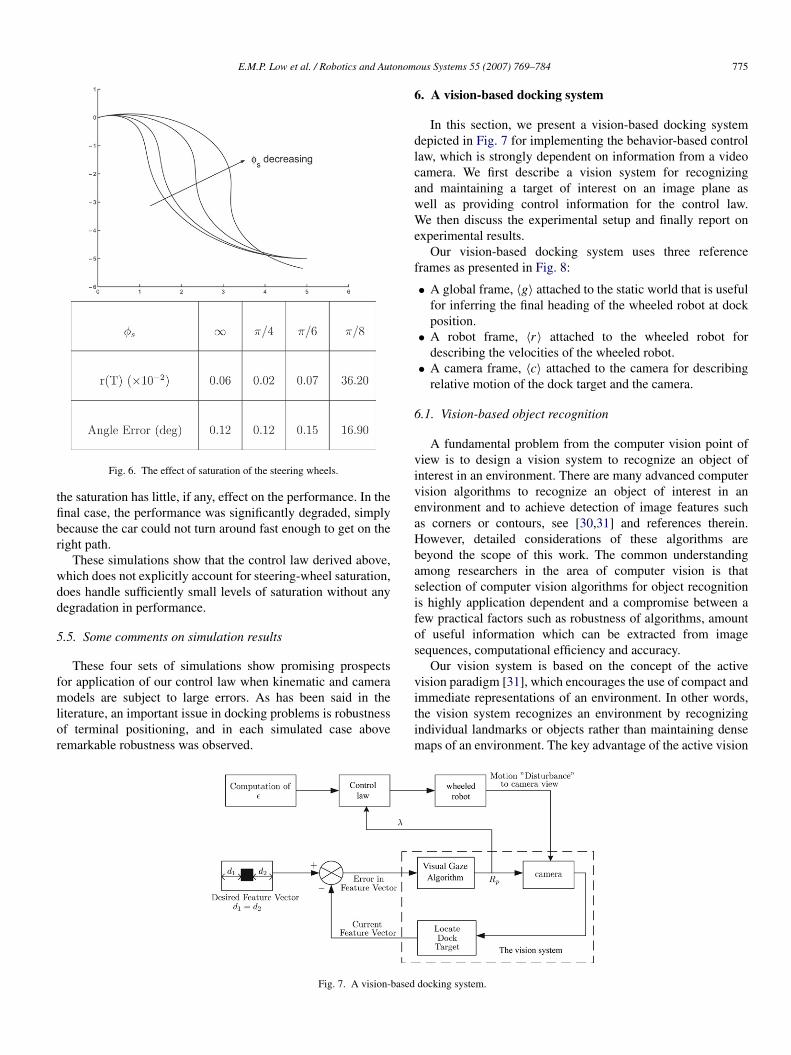
We represent this with the constraint |φ| ≤ φs .In Fig. 6 we depict four trajectories, and four sets of terminal

error data. These are for the cases where, firstly, the steeringwheel angle is not restricted, and then when it is restricted byφs = π/4, π/6, and π/8, respectively. In the first three cases


Fig. 6. The effect of saturation of the steering wheels.

the saturation has little, if any, effect on the performance. In thefinal case, the performance was significantly degraded, simplybecause the car could not turn around fast enough to get on theright path.

These simulations show that the control law derived above,which does not explicitly account for steering-wheel saturation,does handle sufficiently small levels of saturation without anydegradation in performance.

5.5. Some comments on simulation results

These four sets of simulations show promising prospectsfor application of our control law when kinematic and cameramodels are subject to large errors. As has been said in theliterature, an important issue in docking problems is robustnessof terminal positioning, and in each simulated case aboveremarkable robustness was observed.

6. A vision-based docking system

In this section, we present a vision-based docking systemdepicted in Fig. 7 for implementing the behavior-based controllaw, which is strongly dependent on information from a videocamera. We first describe a vision system for recognizingand maintaining a target of interest on an image plane aswell as providing control information for the control law.We then discuss the experimental setup and finally report onexperimental results.

Our vision-based docking system uses three referenceframes as presented in Fig. 8:

• A global frame, g attached to the static world that is usefulfor inferring the final heading of the wheeled robot at dockposition.

• A robot frame, r attached to the wheeled robot fordescribing the velocities of the wheeled robot.

• A camera frame, c attached to the camera for describingrelative motion of the dock target and the camera.

6.1. Vision-based object recognition

A fundamental problem from the computer vision point ofview is to design a vision system to recognize an object ofinterest in an environment. There are many advanced computervision algorithms to recognize an object of interest in anenvironment and to achieve detection of image features suchas corners or contours, see [30,31] and references therein.However, detailed considerations of these algorithms arebeyond the scope of this work. The common understandingamong researchers in the area of computer vision is thatselection of computer vision algorithms for object recognitionis highly application dependent and a compromise between afew practical factors such as robustness of algorithms, amountof useful information which can be extracted from imagesequences, computational efficiency and accuracy.

Our vision system is based on the concept of the activevision paradigm [31], which encourages the use of compact andimmediate representations of an environment. In other words,the vision system recognizes an environment by recognizingindividual landmarks or objects rather than maintaining densemaps of an environment. The key advantage of the active vision

Fig. 7. A vision-based docking system.


Fig. 8. Position of wheeled robot with respect to the global frame.

paradigm is the use of prior knowledge of an object in anenvironment to simplify selection and application of computervision algorithms to image sequences.

To simplify the complexity of selection and computation ofcomputer vision algorithms, we choose the object of interestas a black rectangular cardboard against white backgroundenvironment. We choose the corners of the black rectangularcardboard as image features of interest. As a result, we use acorner detection algorithm [32] in computer vision to detectthe image features. For purposes of completeness, we brieflydescribe the corner detection algorithm in Appendix A.

In practice, directly applying the corner detection algorithmleads to a resultant of too many corners that are not welllocalized, as shown in Fig. 9. We provide an algorithm forachieving good localization of corners.

First, we separate the resultant corners into different clustersbased on a Euclidean distance measure and each cluster willeventually contain a localized corner. The coordinates of thelocalized corner is computed by averaging the coordinates ofall resultant corners in each cluster.

Second, we are interested in detecting only the four cornersof the object, a black rectangular cardboard. To isolate thesecorners, we assume that the object is always maintained withinan adaptive number of pixel rows from the center of the imageplane. All localized corners outside this boundary are regardedas false corners. Then by checking that each vertical side ofthe object will give two localized corners having almost thesame column coordinates will further isolate the right cornersbelonging to the object. Fig. 9 shows four distinct localizedcorners of the object which are subsequently used as feedbackinformation to control the angular rate of a pan video camera tomaintain the object within the camera field of view at all times.Details are given in the following section.

The vision system described in this section is suitable for ex-perimental investigation of various vision-based control strate-

(a) Poor localization of corners.

(b) Good localization of corners.

Fig. 9. Resultant corners computed by corner detection algorithm.

gies in a laboratory setting. Specifically, for experimental in-vestigation of vision-based wheeled robot navigation prob-lems [33] and biologically inspired decentralized control strate-gies, which arise in very recent research in vision-based multi-ple mobile robots coordination [34] and flocking [35,36].


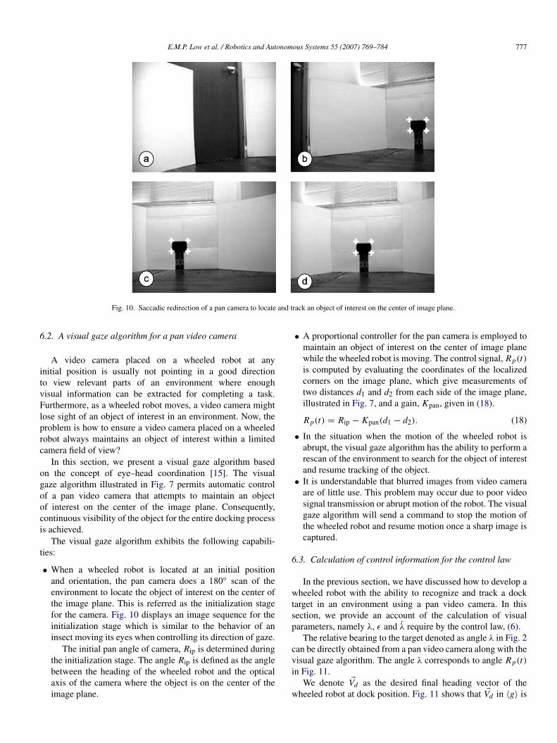
Fig. 10. Saccadic redirection of a pan camera to locate and track an object of interest on the center of image plane.

6.2. A visual gaze algorithm for a pan video camera

A video camera placed on a wheeled robot at anyinitial position is usually not pointing in a good directionto view relevant parts of an environment where enoughvisual information can be extracted for completing a task.Furthermore, as a wheeled robot moves, a video camera mightlose sight of an object of interest in an environment. Now, theproblem is how to ensure a video camera placed on a wheeledrobot always maintains an object of interest within a limitedcamera field of view?

In this section, we present a visual gaze algorithm basedon the concept of eye–head coordination [15]. The visualgaze algorithm illustrated in Fig. 7 permits automatic controlof a pan video camera that attempts to maintain an objectof interest on the center of the image plane. Consequently,continuous visibility of the object for the entire docking processis achieved.

The visual gaze algorithm exhibits the following capabili-ties:

• When a wheeled robot is located at an initial positionand orientation, the pan camera does a 180 scan of theenvironment to locate the object of interest on the center ofthe image plane. This is referred as the initialization stagefor the camera. Fig. 10 displays an image sequence for theinitialization stage which is similar to the behavior of aninsect moving its eyes when controlling its direction of gaze.

The initial pan angle of camera, Rip is determined duringthe initialization stage. The angle Rip is defined as the anglebetween the heading of the wheeled robot and the opticalaxis of the camera where the object is on the center of theimage plane.

• A proportional controller for the pan camera is employed tomaintain an object of interest on the center of image planewhile the wheeled robot is moving. The control signal, Rp(t)is computed by evaluating the coordinates of the localizedcorners on the image plane, which give measurements oftwo distances d1 and d2 from each side of the image plane,illustrated in Fig. 7, and a gain, Kpan, given in (18).

Rp(t) = Rip − Kpan(d1 − d2). (18)

• In the situation when the motion of the wheeled robot isabrupt, the visual gaze algorithm has the ability to perform arescan of the environment to search for the object of interestand resume tracking of the object.

• It is understandable that blurred images from video cameraare of little use. This problem may occur due to poor videosignal transmission or abrupt motion of the robot. The visualgaze algorithm will send a command to stop the motion ofthe wheeled robot and resume motion once a sharp image iscaptured.

6.3. Calculation of control information for the control law

In the previous section, we have discussed how to develop awheeled robot with the ability to recognize and track a docktarget in an environment using a pan video camera. In thissection, we provide an account of the calculation of visualparameters, namely λ, and λ require by the control law, (6).

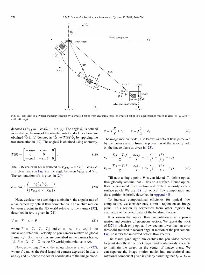
The relative bearing to the target denoted as angle λ in Fig. 2can be directly obtained from a pan video camera along with thevisual gaze algorithm. The angle λ corresponds to angle Rp(t)in Fig. 11.

We denote Vd as the desired final heading vector of thewheeled robot at dock position. Fig. 11 shows that Vd in g is


Fig. 11. Top view of a typical trajectory execute by a wheeled robot from any initial pose of wheeled robot to a dock position which is close to (x, y, θ) =(∼0, ∼0, ∼θd ).

denoted as Vdg = − cos θd i + sin θd j . The angle θd is definedas an abstract bearing of the wheeled robot at dock position. Weobtained Vd in c denoted as Vdc = T (θ) Vdg by applying thetransformation in (19). The angle θ is obtained using odometry.

T (θ) =

− sin θ cos θ 0

0 0 1− cos θ − sin θ 0

. (19)

The LOS vector in c is denoted as VLOSc = sin λ i + cos λ k.It is clear that in Fig. 2 is the angle between VLOSc and Vdc.The computation of is given in (20).

= cos−1

VLOSc Vdc

VLOSc × Vdc

. (20)

Next, we describe a technique to obtain λ, the angular rate ofa pan camera by optical flow computation. The relative motionbetween a point in the 3D world relative to the camera [32],described in c, is given in (21).

V = −T − ω × P (21)

where T =Tx Ty Tz

and ω =

ωx ωy ωz

is the

linear and rotational velocity of pan camera relative to globalframe, g. Both velocities are described in the camera frame,c. P =

X Y Z

is the 3D world point relative to c.

Now, projecting P onto the image plane is given by (22),where f denotes the focal length of camera expressed in pixelsand cx and cy denote the center coordinates of the image plane.

x = fXZ

+ cx y = fYZ

+ cy . (22)

The image motion model, also known as optical flow, perceivedby the camera results from the projection of the velocity fieldon the image plane as given in (23).

vx = Tz x − Tx fZ

+ ωx xyf

− ωy

f + x2

f

+ ωz y

vy = Tz y − Ty fZ

− ωy xyf

+ ωx

f + y2

f

− ωz x . (23)

Till now a single point, P is considered. To define opticalflow globally, assume that P lies on a surface. Hence opticalflow is generated from motion and texture intensity over asurface patch. We use [28] for optical flow computation andthe algorithm is briefly described in Appendix B.

To increase computational efficiency for optical flowcomputation, we consider only a small region on an imageplane. This region is segmented from other regions byevaluation of the coordinates of the localized corners.

It is known that optical flow computation is an approxi-mation and consists of erroneous vectors. We repeat the workof [37] in which only optical flow vectors lower than an errorthreshold are used to recover angular motion of the pan camera.Fig. 12 shows the improved optical flow vectors.

The visual gaze algorithm enables the pan video camerato point directly at the dock target and continuously attemptsto maintain the target on the center of image plane. Wecan separate the image motion model into translational androtational component given in (24) by assuming that Tx = Ty =


(a) Noisy optical flow vectors before thresholding. (b) Noisy optical flow vectors before thresholding.

(c) Improved optical flow vectors after thresholding. (d) Improved optical flow vectors after thresholding.

Fig. 12. Optical flow vectors over a surface patch with translational motion.

ωx = ωz = 0.

vx = Tz xZ

− Ωx , Ωx = ωy(1 + x2)

vy = Tz yZ

− Ωy, Ωy = ωy xy.

(24)

We recover λ, which is represented as ωy , by choosinga region, R, on the image plane where there is sufficientcorrectness of optical flow vectors based on least squaremethods in (25).

ωy =

R

(vy xy − vx y2)

R

y2 . (25)

Lastly, it is required to stop the wheeled robot in front ofthe dock target. The image of the dock target gets bigger asthe wheeled robot moves toward it. The distance between thelocalized corners of the dock target on the image plane givesan indication of the actual distance between the wheeled robotrelative to the dock target in g. We use this information to stopthe wheeled robot when it is approaching near the dock target.

6.4. Experimental setup

The proposed control law was experimentally verified usingthe vision-based docking system in Fig. 7. This sectiondescribes the experimental setup and reports the results.

The experiments were carried out on a Pioneer 3 wheeledrobot from ActivMedia. The wheeled robot is equippedwith a pan-tilt-zoom (PTZ) color video camera. The controlalgorithms operate at a calculation period of 0.5 s, computervision algorithms and data logger were implemented in C++with the ARIA [38] software development environment runningin the Linux operating system. A resolution of 320×240 pixelswas selected for image processing.

A simplified version of the control law in (6) wasinvestigated by experiments using a unicycle wheeled robot,shown in Fig. 13. In this case, the proposed control law becomesω := u = aec + beh . We are concerned with controlling theturning rate of the wheeled robot. The following parameterswere used, Kpan = 0.16, a = 0.1 and b = 0.32 and thelinear velocity of the wheeled robot is v = 0.1 m/s. The v

and ω of the wheeled robot are related to the velocity of theleft and right wheel of the wheeled robot by ωl = v − lω andωr = v + lω respectively, where l is half the distance betweenthe two wheels.

6.5. Experimental results

Experimental results are presented for two cases wherethe wheeled robot was located at initial pose of (x, y, θ) =(3.0 m, 0.72 m, π

2 ) and (x, y, θ) = (2.6 m, 0.82 m, π2 )

respectively. The objective of the experiments was to dock thewheeled robot in front of the target which corresponds to a


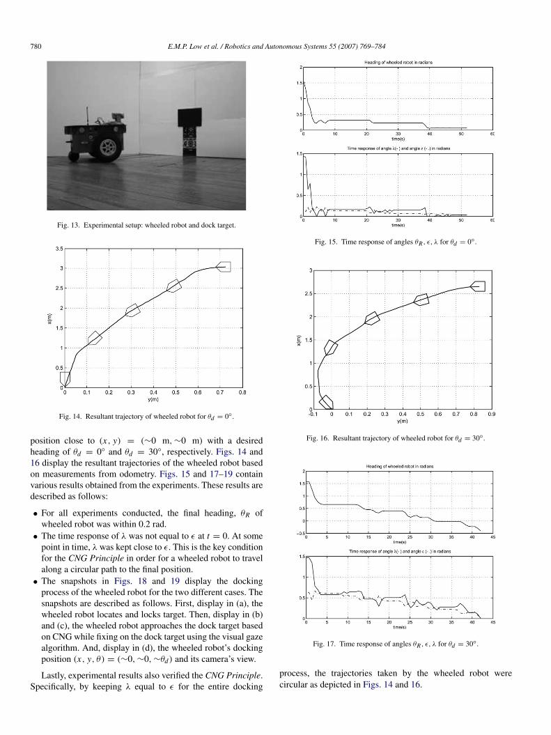
Fig. 13. Experimental setup: wheeled robot and dock target.

Fig. 14. Resultant trajectory of wheeled robot for θd = 0.

position close to (x, y) = (∼0 m, ∼0 m) with a desiredheading of θd = 0 and θd = 30, respectively. Figs. 14 and16 display the resultant trajectories of the wheeled robot basedon measurements from odometry. Figs. 15 and 17–19 containvarious results obtained from the experiments. These results aredescribed as follows:

• For all experiments conducted, the final heading, θR ofwheeled robot was within 0.2 rad.

• The time response of λ was not equal to at t = 0. At somepoint in time, λ was kept close to . This is the key conditionfor the CNG Principle in order for a wheeled robot to travelalong a circular path to the final position.

• The snapshots in Figs. 18 and 19 display the dockingprocess of the wheeled robot for the two different cases. Thesnapshots are described as follows. First, display in (a), thewheeled robot locates and locks target. Then, display in (b)and (c), the wheeled robot approaches the dock target basedon CNG while fixing on the dock target using the visual gazealgorithm. And, display in (d), the wheeled robot’s dockingposition (x, y, θ) = (∼0, ∼0, ∼θd) and its camera’s view.

Lastly, experimental results also verified the CNG Principle.Specifically, by keeping λ equal to for the entire docking

Fig. 15. Time response of angles θR , , λ for θd = 0.

Fig. 16. Resultant trajectory of wheeled robot for θd = 30.

Fig. 17. Time response of angles θR , , λ for θd = 30.

process, the trajectories taken by the wheeled robot werecircular as depicted in Figs. 14 and 16.


Fig. 18. Snapshots of the docking process for θd = 0.

7. Conclusion

We have presented a vision-based docking system forcontrolling a wheeled robot to perform docking. The dockingsystem consists of a behavior-based control law based on anavigation technique called the CNG Principle and a visionsystem design. The behavior-based control law is stronglydependent on information from a video camera. We havedescribed a vision system design that consists of pan videocamera and a visual gaze algorithm which mimics behaviorof insects. Also, computer vision algorithms are presented torecognize objects of interest and to compute visual parametersrequired by the behavior-based control law. The vision-based docking system was experimentally investigated using awheeled robot and a pan video camera in a laboratory setting.

Experimental results verified the applicability of the control lawand the concept of the navigation technique. We believe thatthe vision-based docking system would have applications tomanufacturing industries and autonomous highway systems.

Appendix A. Algorithm for corner detection

For each image frame, I (x, y), the following is required todetect whether a given pixel (x, y) is a corner feature:

• Compute the image intensity gradient in the vertical andhorizontal direction, (Ix , Iy), using the gradient filter. Theimage intensity gradient is shown in Fig. A.1.

• Let W be a square region of support of N × N pixels(typically, N = 5). At every image point, (x, y), compute


Fig. 19. Snapshots of the docking process for θd = 30.

the matrix, (A.1), using all pixels in the window, W .

M =

pi∈WIx (pi )

pi∈WIx (pi )Iy(pi )

pi∈WIy(pi )Ix (pi )

pi∈WIy(pi )

. (A.1)

This matrix characterizes the structure of the grey level inM . This is given in the eigenvalues, λ1 and λ2, of M and itsgeometric interpretation.

If λ1 = λ2 = 0, it implies no intensity change in W . Ifλ1 > 0 and λ2 = 0, it implies strong gradient change in onedirection in W .

If the smallest eigenvalue, λ1 ≥ λ2 > 0 of matrix Mand λ2 is greater than a prefixed threshold, τ , then the pixel,(x, y), is considered a corner.

Appendix B. Algorithm for optical flow

Applying Lucas and Kanade, [28], the input is a time-varying sequence of n images, E1, E2, . . . , En . Let Q be asquare region of support of N × N pixels (typically, N = 5).• Prefilter each image with a Gaussian filter of standard

deviation, σ = 1.5 along each dimension.• The optical flow can be estimated within Q as the constant

vector, v, that minimizes the function in (B.1).

ξ [v] =

pi∈Q[(∇E)Tv + Et ]2 (B.1)

where pi is each point within the N × N patch, Q.The solution to this least squares problem is given in

(B.2).

v =vxvy

= (AT A)−1 ATb (B.2)


(a) Original image frame.

(b) Intensity gradient in the x-direction.

(c) Intensity gradient in the y-direction.

Fig. A.1. Image intensity gradients.

where

A =

∇E(p1)∇E(p2)

...

∇E(pN x N )

(B.3)

and

b =Et (p1) Et (p2) · · · Et (pN x N )

. (B.4)

References

[1] R.C. Arkin, Behaviour-based Robotics, MIT Press, Cambridge, MA,1998.

[2] M.O. Franz, H.A. Mallot, Biomimetic robot navigation, Robotics andAutonomous Systems 30 (2000) 133–153.

[3] S. Hutchinson, G.D. Hager, P.I. Corke, A tutorial on visual servo control,IEEE Transactions on Robotics and Automation 12 (5) (1996) 651–670.

[4] I.R. Manchester, A.V. Savkin, Circular navigation guidance law forprecision missile target engagements, Journal of Guidance, Control, andDynamics 29 (2) (2006).

[5] A.V. Savkin, P.N. Pathirana, F.A. Faruqi, The problem of precision missileguidance: LQR and H∞ frameworks, IEEE Transactions on Aerospaceand Electronic Systems 39 (3) (2003) 901–910.

[6] I.R. Petersen, V.A. Ugrinovskii, A.V. Savkin, Robust Control Designusing H∞ Methods, Springer-Verlag, London, 2000.

[7] I.R. Petersen, A.V. Savkin, Robust Kalman Filtering for Signals andSystems with Large Uncertainties, Birkhauser, Boston, MA, 1999.

[8] A.V. Savkin, I.R. Petersen, A connection between H-infinity control andabsolute stabilizability of uncertain systems, Systems and Control Letters23 (1994) 197–203.

[9] A.V. Savkin, I.R. Petersen, Nonlinear versus linear control in the absolutestabilizability of uncertain linear systems with structured uncertainty,IEEE Transactions on Automatic Control 40 (1) (1995) 122–127.

[10] A.V. Savkin, I.R. Petersen, Recursive state estimation for uncertainsystems with an integral quadratic constraint, IEEE Transactions onAutomatic Control 40 (6) (1995) 1080–1083.

[11] M.V. Srinivasan, S.W. Zhang, J.S. Chahl, E. Barth, S. Venkatesh, Howhoneybees make grazing landings on flat surfaces, Biological Cybernetics83 (2000) 171–183.

[12] M.V. Srinivasan, S.W. Zhang, M. Lehrer, T.S. Collett, Honeybeenavigation en route to the goal: Visual flight control and odometry, Journalof Experimental Biology 199 (1996) 237–244.

[13] G.L. Barrows, J.S. Chahl, M.V. Srinivasan, Biomimetic visual sensing andflight control, Aeronautical Journal 107 (1069) (2003) 159–168.

[14] I.R. Manchester, A.V. Savkin, Vision-based docking for biomimeticwheeled robots, in: Proceedings of the 15th IFAC World Congress,Prague, Czech Republic, July 2005.

[15] G. Cannata, E. Grosso, On perceptual advantages of active robot vision,Journal of Robotic Systems 16 (3) (1999) 163–183.

[16] E.M.P. Low, I.R. Manchester, A.V. Savkin, A method for vision-based docking of wheeled mobile robots, in: Proceedings of the IEEEInternational Conference on Control Applications, Munich, Germany,October 2006.

[17] B.K.P. Horn, Robot Vision, The MIT Press, Cambridge, MA, 1986.[18] C. Canudis de Wit, O.J. Sørdalen, Exponential stabilization of mobile

robots with nonholonomic constraints, IEEE Transactions on AutomaticControl 37 (11) (1992) 1791–1797.

[19] J.P. Laumond (Ed.), Robot Motion Planning and Control, Springer-Verlag,New York, NY, 1998.

[20] P. Soueres, J.P. Laumond, Shortest paths synthesis for a car-like robot,IEEE Transactions on Automatic Control 41 (5) (1996) 672–688.

[21] A. Kelly, B. Nagy, Reactive nonholonomic trajectory generation viaparametric optimal control, International Journal of Robotics Research 22(7) (2003) 583–601.

[22] J. Santos-Victor, G. Sandini, Divergent stereo in autonomous navigation:From bees to robots, International Journal of Computer Vision 14 (1995)159–177.

[23] K. Hashimoto, T. Noritsugu, Visual servoing of nonholonomic cart, in:IEEE International Conference on Robotics and Automation, April 1997,pp. 1719–1724.

[24] S. Lee, M. Kim, Y. Youm, W. Chung, Control of a car-like mobile robotfor parking problem, in: IEEE International Conference on Robotics andAutomation, September 1999, pp. 1–6.

[25] F. Conticelli, B. Allotta, P.K. Khosla, Image-based visual servoing ofnonholonomic mobile robots, in: 38th IEEE Conference on Decision andControl, December 1999, pp. 3496–3501.

[26] H. Zhang, J.P. Ostrowski, Visual motion planning for mobile robots, IEEETransactions on Robotics and Automation 18 (2) (2002) 199–208.

[27] A. Cardenas, B. Goodwin, S. Skaar, M. Seelinger, Vision-based controlof a mobile base and on-board arm, International Journal of RoboticsResearch 22 (9) (2003) 677–698.

[28] B. Lucas, T. Kanade, An iterative image registration technique withan application to stereo vision, in: Proceedings of DARPA ImageUnderstanding Workshop, 1981, pp. 121–130.

[29] H.K. Khalil, Nonlinear Systems, 3rd ed., Prentice Hall, Upper SaddleRiver, NJ, 2002.


[30] C. Tomasi, T. Kanade, Detection and tracking of point features, CarnegieMellon University, Pittsburgh, PA, Tech. Rep. CMU-CS-91-132, April,1991.

[31] A. Blake, M. Isard, Active Contours, Springer-Verlag, 1998.[32] Y. Ma, S. Soatto, J. Kosecka, S.S. Sastry, An Invitation to 3-D Vision,

Springer-Verlag, New York, NY, 2004.[33] I.R. Manchester, E.M.P. Low, A.V. Savkin, Vision-based interception of a

moving target by a mobile robot, in: Proceedings of the IEEE InternationalConference on Control Applications, Singapore, October 2007.

[34] N. Moshtagh, A. Jadbabaie, K. Daniilidis, Vision-based control laws fordistributed flocking of nonholonomic agents, in: Proceedings of the IEEEInternational Conference on Robotics and Automation, Orlando, FL, May2006.

[35] A. Jadbabaie, J. Lin, A.S. Morse, Coordination of groups of mobileautonomous agents using nearest neighbor rules, IEEE Transactions onAutomatic Control 48 (6) (2003) 998–1001.

[36] A.V. Savkin, Coordinated collective motion of groups of autonomousmobile robots: Analysis of Vicsek’s model, IEEE Transactions onAutomatic Control 49 (6) (2004) 981–982.

[37] A. Dev, B.J.A. Krose, F.C.A. Groen, Confidence measure for imagemotion estimation, in: Proceedings 1997 RWC Symposium, RWCTechnical Report TR - 96001, 1997, pp. 199–206.

[38] ActivMedia, http://www.activmedia.com/.

Emily Low was born in 1979 in Singapore. She iscurrently a Ph.D. candidate in Electrical Engineering atthe University of New South Wales, Sydney, Australia.She received her B.E. (Hons 1) degree in 2003from Nanyang Technological University, Singapore.From 1999 to 2000, she worked as technologiston navigation techology in the Defence ScienceOrganization, Singapore. From 2003 to 2004, sheworked as software engineer on smart card techologyin Gemplus Technologies Asia. Her current research

interests include vision-based navigation and control of mobile robots.

Ian R. Manchester was born in Sydney, Australia,in 1979. He completed the B.E. (Hons 1) degree in2001 and the Ph.D. degree in 2005, both in ElectricalEngineering at the University of New South Wales,Sydney, Australia. Since 2005 he has held a post-doctoral position in the control systems group at theDepartment of Applied Physics and Electronics, UmeUniversity, Ume, Sweden. In 2006 he spent a monthas a visiting researcher at the Intelligent SystemsResearch Centre, Sungkyunkwan University, Suwon,

South Korea. His current research interests include vision-based guidance androbotics, control of underactuated and non-holonomic systems, and modellingand identification of the human cerebrospinal fluid system. He has publishedseveral journal and conference articles on these topics.

Andrey V. Savkin was born in 1965 in Norilsk, USSR.He received the M.S. degree (1987) and the Ph.D.degree (1991) from The Leningrad University, USSR.From 1987 to 1992, he worked in the All-UnionTelevision Research Institute, Leningrad. From 1992 to1994, he held a postdoctoral position in the Departmentof Electrical Engineering, Australian Defence ForceAcademy, Canberra. From 1994 to 1996, he was aResearch Fellow with the Department of Electrical andElectronic Engineering and the Cooperative Research

Center for Sensor Signal and Information Processing at the University ofMelbourne, Australia. Since 1996, he has been a Senior Lecturer, and thenan Associate Professor with the Department of Electrical and ElectronicEngineering at the University of Western Australia, Perth. Since 2000,he has been a Professor with the School of Electrical Engineering andTelecommunications, The University of New South Wales, Sydney.

His current research interests include robust control and filtering, hybriddynamical systems, missile guidance, networked control systems, computer-integrated manufacturing, control of mobile robots, computer vision, andapplication of control and signal processing to biomedical engineering andmedicine. He has published four books and numerous journal and conferencepapers on these topics and served as an Associate Editor for severalinternational journals and conferences.

http://www.activmedia.com/

a biologically inspired method for vision-based docking of

Documents