A Composite DiscretdContinuous Control of Robot Manipulators

Ju-Jang Lee and Yangsheng Xu

CMU-RI-TR-91-09

The Robotics Institute Carnegie Mellon Univerrity

Pitrsbqh, F'e~sylvania 15213

A@ 1991

@ Camegie Meum University

Contents

1 Introduction

2 Preliminaries

3 Composite Control Algorithm

4 Simulation Results

5 Conclusions

Acknowledgements

References

14

21

22

23

List of Tables

1 The Computational Cost Summaryof Feedback Control Component Using the Proposed Algorithm . . . . . . . . . . . . . . . . . . . . . 13

2 Simulation Results of the Proposed Algorithm . . . . . . . . . . . . 19

ii

List of Figures

I A Three Degree-of-Freedom Manipulator . . . . . . . . . . . . . . . 14

2 Block Diagram of the Computed Torque Method . . . . . . . . . . . 15 3 Block Diagram of the Proposed Control Algorithms . . . . . . . . . 15 4 Simulation Results of CTM Algorithm . . . . . . . . . . . . . . . . 16 5 Simulation h u l t s of Theorem 1 . . . . . . . . . . . . . . . . . . . 17 6 Simulation Results of Theorem 2 . . . . . . . . . . . . . . . . . . . 18

... 111

.- ........... .. ............

.-

ABSTRACT

In this report, a composite control scheme for the control of robot manipula- tors is proposed.

Due to the modeling error or environmental uncertainties, robot motion may present a significant positioning error by using a conventional Computer-Torque Method. To improve tracking capability of robot manipulators, sliding mode control and nonlinear control algorithms have been introduced, but computation is costly, and thus a fast motion execution using simple computer sources is impossible.

To solve this problem, we present a composite control algorithm to control robot motion combining a discrete feedforward component and a continuous feed- back component. The discrete feedforward component provides a nominal torque computed using the robot dynamics and compensates for dynamic coupling be- tween the links. This part can be updated in a luge sampling time, and can be computed off-line generally, thus real time computation is decreased. The continuous feedback control component uses a structure of Variable Structure System and provides a robust control to disturbances during the sliding mode. This part can be digitally implemented using a short sampling time, and thus a fast motion of a multi-degree freedom robot manipulator can be executed by using a simple computer, or even a single board computer with an %bit CPU.

The stability of the proposed multiple-rate control scheme is proven in the paper and efficiency of the control scheme has been demonstrated by simulations of a three-link robot subject to parameter and payload uncertainties.

- ~~~. ...~. . -. . .. .. . . . . . .

1 Introduction The lack of efficient and robust real-time control algorithms for high speed motions is one of the important reasons why the applications of the present robotic manipulators are lim- ited. The dynamic equation of robotic manipulator is highly nonlinear due to the inertia and strong coupling terms among the joints, such as centrifugal, Coriolis and gravitational forces [ l l , 121. It is difficult to guarantee the tracking error bound in high speed motion, by neglecting the nonlinear dynamic terms which may act as a large disturbance to the controller. In order to improve the trajectory tracking accuracy, it is necessary to take the robot manipulator dynamics into consideration [12].

The well-known Computed Torque Method (CTM) normally provides a feasible controller if the exact knowledge of the manipulator dynamics is available. However, for a large amount of applications, it is impossible to obtain the complete dynamic model of robots, due to modeling uncertainties, parameter variation and unknown payloads. These uncertainties, especially the error of inertia matrix, may result in the instability of robot systems [ l T , 131. On the other hand, the computation time of such a complex dynamics also makes its implementation impractical in some cases.

The sliding mode controller based on the Variable Structure System (VSS) method has the properties of rejection to disturbance and insensitivity to parameter variations. The method does not need to have a complete knowledge of the accurate model, and only knowl- edge required is the bounds of uncertain parameters of the system for the design of the controller [IS]. These two features are exactly the merits for the control of a manipulator which is subjected to the modeling uncertainties and large disturbances. Therefore, the sliding mode control [lo, 6, 4, 51 has been proposed in many robot control algorithms.

Depending on the side of the hyperplane (Le., sliding surface) that the system belongs to, the VSS is of two structures. If the control structure can be switched with an ideally infinite frequency, the motion of the controlled system remains on the sliding surface. Then, the system is governed by dynamics of the sliding surface only, and the system is insensitive to parameter variations and disturbances. However, an ideal switching of the input with an infinite frequency is practically impossible due to the switching delays and neglecting time constants. Instead, the control input switches with a finite high frequency and the motion of the system is within some neighborhood of the sliding surface with chattering. This chattering is generally undesirable in practice, since it involves extremely high control activity and thereby excites the high frequency dynamics that is neglected in the model.

To solve this problem, various algorithms have been proposed to replace the discontinuous control in neighborhood of the sliding surface by the continuous control [6, 4, 51, such as the VSS algorithm, if the trajectory is outside the boundary of the sliding surface. If the trajectory is within the boundary of the sliding surface, however, a lot of people suggested to interpolate the control by proper continuous function to minimize the chattering caused by a switching input. In the implementation of these algorithms digitally, we need to compute robot model and feedback of position and velocity at every sampling time. In spite of the efficient recursive dynamic algorithms [ l l , 12, 81 and computing architectures [15], the computation of the model is relatively more costly. The time delay of control input, due to the computation time, deteriorates the performance in real-time control systems 191.

1

To reduce the time delay of control, it is desirable that the feedback is not involved in computation of the model, and the feedforward compensation using the nominal torque is good in this sense [3, I]. The adaptive control algorithm with feedforward compensation provides a robust method to control robot manipulators. Actually there are a lot papers about the stability of the adaptive control. The feedback component of the adaptive control needs a considerable amount of computation. We believe that the composite controller com- bining the discrete feedforward and continuous feedback controls provides a good trajectory tracking performance in the real-time implementation.

In this paper, a composite control algorithm is proposed and the stability of the system is proven. The proposed algorithm is comprised of discrete and continuous control loops. The discrete feedforward component provides a nominal torque computed using robot dynamics and compensates for dynamic coupling between the links. This part can be updated in a large sampling time, and can be computed off-line generally, thus a real time computation is infeasible. The continuous feedback control component uses a structure of Variable Structure System and provides a robust control to disturbances of the system during the sliding mode. This part can be digitally implemented using a short sampling time, and thus a fast motion of a multi-degree freedom robot manipulator can be executed by using a simple computer, or even a single board computer with an 8-bit CPU.

The rest of the paper is organized as follows. In Section 2, we describe preliminary Lemmas as a preparation for the main control algorithms. In Section 3, we present a new composite control algorithm with proofs. In Section 4, the efficiency of the proposed algo- rithm for the position control is demonstrated by the simulation of a three degrees-of-freedom manipulator. The robust property to the modeling errors, the time delay of computation, pa- rameter uncertainties and payload variations is discussed. We conclude the paper in Section 5.

2

2 Preliminaries The motion equations of an n degree-of-freedom (d.0.f.) manipulator can be derived using the Lagrange-Euler formulation as

where ~ ( t ) E R" is a joint input torque vector; q( t ) ,g ( t ) , t ( t ) E R" are the generalized position, velocity and acceleration vectors of the joint angles; D ( q ( t ) ) E RnX" is a symmetric positive definite inertia matrix, and h(q( t ) , i ( t ) ) E R" is a nonlinear coupling vector including centrifugal, Coriolis and gravitational forces 12). In the following, we denote D(q( t ) ) by D and h(q( t ) , i ( t ) ) by h for brevity.

Let us define the state vector z ( t ) E R2" as

Then the state equation of the robot system is

Given the desired trajectories q d ( t ) , &(t) , &(t) E R" and initial time to, we define the sliding surface vector s(t) f R" as

1 s ( t ) = i ( t ) + K,e(t) + K p 1 e(7)dT (4) to

where e(t) = q( t ) - q d ( t ) is an error vector in joint space and K,,K6 E R"'" are gain matrices. For the use of the following derivation, we introduce intermediate trajectories, q*(t), i * ( t ) , &(t) E R", which satisfies the following equation

Z ( t ) + K.k(t) + K,e(t) = 0. (5)

Then we can rewrite (5) as follows

k*(t) - k,j(t) = A . [ ~ . ( l ) - ~ d ( t ) ] (6)

where ~ . ( t ) = [q*(t)T,i.(t)TJT E RZn, a ( t ) = [ q d ( t ) T , q d ( t ) T ] T E R2" and A E Rznxlrn is

0 ( 7 )

Since del[XZ-A] = det[X21+XK,+KpJ, we can choose K, and K p so that all the eigenvalues of the matrix A have negative real parts, which guarantees the exponential stability of the system ( 6 ) , and then there exist g > 0 and n > 0 such that

3

for all t 2 0 [IS]. Here, the Euclidean matrix norm of A is defined as

IlAll = [ h ( A ' A ) ] i (9)

where AM(.) denotes the maximum eigenvalue of a matrix. Now, we will state the following two Lemmas as a prerequisite to the main theorems.

Lemma 1 : If the sliding surface defined by Equation (4) satisfies Ils(t)ll 5 7 for any t 2 to, then

Ilz(t) - z.(t)ll 5 [Ilx(t,) - z*(to)l + 271 . ellAll'

is satisfied for all t 2 1,. Proof : Using (4) and ( 6 ) , we may rewrite (3) as

i ( t ) - k*(t) = A . [ ~ ( t ) - ~ . ( t ) ] + (11)

Integrating both sides of (11) yields

Taking the norm of both sides, we get

Ilz(t) - z.(t)ll I [Ilz(tJ - z*(to)ll + 271 + /tIIAll .IIz(.) - 4T)IldT. (13) t o

If we apply the Bellman-Gronwall Inequality [14] t o (13), we obtain

~lr( t ) - z.(t)ll 5 [llz(to) - Z*(L)II + 271 . ellAllt (14)

for all t 2 to, and thus Lemma 1 is true. If we take z.(to) = z(to) at the initial time, Equation (IO) becomes

Il+(t) - z.(t)ll 5 27 . ellAll*. (15)

The above Lemma implies that the distance from red trajectory z( t ) to the intermediate trajectory s.(t) is bounded for a finite time. The Lemma 2 below shows that the boundness of the tracking error holds also for an infinite time interval. Considering p as a positive number and vector u E Rn,,we defme the neighborhood set as follows

S(p; u) = {w E R"; llw - VI1 5 p } . (16)

Lemma 2 : Suppose I ls(t) l l 5 y is satisfied for all t 1 to for some to, and the system (6) is exponentially stable and satisfies (8). Then z(t) converges exponentially into the set S(q;zd( t ) ) with t which is given by

4

where p is defined as

Proof : Since the intermediate trajectory satisfies (8), there exists T = T(a) < 03

T = - ln(a/s) n (19)

= B . ll4L4 - S d ( b ) l l . (23) Now if ( (s( t ) - r d ( l ) l l > E(a, 8) . 7 holds for t = to + T, we repeat the previous process with the initial condition z.(t. + T) = z(t. + T) at time t = t , + T . Then

(lz(to + 2T) - z d ( t o + 2T)Il < B ' Ilx(to f T ) - Z d ( t a + T)ll

< p a ' I l s ( i o ) - r d ( t s ) l l .

I l z ( to + "T) - 2 d ( t o + nT)II < B" . Ilr(to) - I d ( t o ) l l .

(24)

(25)

If this process is repeated n times, we have

Equation (25) implies the exponential convergence of ~ ( t ) into the set S(E(a , p ) ; zd ( t ) ) . It remains to find out the supremum of the trajectory errors for all Q and p with the

constraint 0 < a < ,@ < 1. Clearly, the infimum of E ( u , p ) with respect to p occurs as P --t

1. and this results in

We differentiate E(a , 1 ) with respect to CY and let the derivative be equal to 0, i.e.,

- = 0. d E ( a , l ) - 2(l/g)(a/g)-'eU+'). ((1 + CY - +}

d a (1 -CY) ' (27)

5

We can obtain the minimum of E(a, 1) when

and the upper bound of the trajectory error, t = E ( a * , l ) , is given by (17) and (18). This completes the proof of Lemma 2.

Note that the equivalent trajectory is only a virtual intermediate function between ~ ( t ) and Zd(t) and does not exist in a real system. If Ilz(to) - sd(to)ll 5 e . y is satisfied at the initial time t = to, then the system trajectory satisfies Ils(t) - zd(t)ll 5 t . 7 for all t > to. In the next section, we will propose a controller which guarantees Ils(t)ll I: y, then the trajectory error is bounded in virtue of Lemma 2.

3 Composite Control Algorithm To compute the input torque using the nonlinear control algorithms, we need the dynamic model of a robot system. For many cases an exact model is impossible due to the parameter uncertainties and payloads variations. Therefore, we express the model of the robot system (1) as follows

m t ) ) .4w + &dt),4(t)) = d t ) (28) where b(q(t)) . ;i(t) and i (q( t ) ) , t j ( t ) ) represent the corresponding terms of the real system (1) with modeled values of the parameters.

In general, we may consider the control as two parts, a feedforward term and a feedback term, Le.,

T ( t ) = rfj(1) + T c ( ~ ) (29)

The feedforward term ~ j j ( t ) and the premultiplying coefficient, b ( q d ( t ) ) of the feedback term ~ ~ ( t ) can be computed in off-line, and thus are step functions with time interval To which is supposedly greater than the necessary computation time for the model (28). In spite of the development of various algorithms and enhancements of computing architectures, com- putation of the model is still costly and thus the required time interval To is still not small. We used the notations &(t) , a d ( t ) , i d ( t ) to denote the sampled values of the correspond- ing desired trajectories q d ( t ) , C j d ( t ) , i d ( t ) with a sampling internal To (i.e., q d ( t ) = q d ( k T p ) , Gd(t) = q d ( k T p ) , and c d ( t ) = G d ( k T p ) for dl t E [kTp,(k + 1)Tp)) . For brevity, b ( Q d ( t ) ) is denoted by b d and i ( q d ( t ) , & ( t ) ) by i d . If the robot system (1) is controlled by the input torque computed by (29)-(32), we obtain

-

7

Define the constants N and M as such

In what follows, we prove the stability of the system using the controller given by (29)- (32).

Theorem 1 : For a robotic system (1) using controller given by (29)- (32), if at the initial time t = to for any 7 > 0,

and the gain ko is bounded by

for the given K,, K,, IC. and for a small positive p , then the system tracking error satisfies

I l s ( t ) l l 5 7 3 E S ( f 7 ; z d ( t ) ) (40)

for all t 2 to. Proof : We consider V ( t ) = $s( t )Ts( t ) as a Lyapunov function and differentiate it with

Using the matrix inequality 171,

we obtain

If we assume that z( t ) # S(c7;zd(t)) for some t = t z , there exists tl E [ to , t2 ) such that s ( t ) E S(7) for all t E [t, ,ti) and Ils(t1)ll = 7, since Ilz(t,) - z d ( t o ) l l 5 e . 7 and the motion trajectory is continuous. Then r(t1) E S(q; z d ( t l ) ) is satisfied (from Lemma 2), and Iln(h)ll 5 N and Il6D(ti)ll L M are satisfied from the definitions of (37) and (38). Hence, we can rewrite (43) as

8

at t = tl. If the gain I s , satisfies the condition (39), then

dV dt - ( t ) < - p ' s(t)Ts(t) (45)

at t = t l , which contradicts the assumption that s ( t ) # S(q;zd(t)). This completes the proof of Theorem 1.

If we use a small sampling time T p and have a relatively accurate model, then the maximum values of N and M can be small. In this case, the lower bound of k, can be made to be small and the upper bound of ko can be made to be large enough to ensure the existence of the gain k,,. Since the role of feedforward component . r j j ( t ) is compensation for the dynamics and nonlinear coupling torques between the joints, we may take a large sampling time To for the discrete terms b d and i d to reduce the computation. Of course, the sampling time should not be too large. With increase of the sampling time, the magnitude of modeling errors, Iln(t)ll and IlbD(t)ll may become large, and thus the required bounds of the gain ko become severe and the trajectory error is increased. This will be discussed in detail in Section 4.

Using the smaller 7, s ( t ) remains closer to the surface s ( t ) = 0 and the trajectory error becomes smaller. In this case, the lower bound of the gain ko is not necessarily increased since the constant N of (37) is decreased. If we take the smaller A in the control algorithm (32), then both the lower and upper bounds of the gain ko are decreased. However, it is difficult to expect that the control changes smoothly.

In order to achieve a smooth change of control output, we may consider the interpolation of the discrete terms b d and h d in (30) and (31). Since these terms are functions of the desired trajectories and can be computed in off-line, the interpolation of these terms can be achieved by various simple methods.

Substituting the continuous feedback terms q(t ) and q(t) to the sampled nominal tra- jectory q d ( t ) and &(t) , we may get the continuous control input in a combined form as follows

70) = &z(t)) ' 4 t ) + M t ) , 4.(t)) (46)

Then, we can prove the bounddness of the tracking errors of the system (1) by the controller (46) and (47) in the same manner as in Theorem 1.

If the model is relatively accurate and the sampling time of discrete components (To) is small, it is not so severe to aSsume that M < 1. In this case, we can obtain the following Corollary which gives another condition for ko.

Corollary 1 : Consider the robot system (1) using the controller given by (29)-(32). If M < 1 and at the initial time t = to, Ils(t.)l] 5 7 and Ils(t,) - Zd( to ) l l 5 e . y for any y > 0 is satisfied at the initial time to, and if the gain k, is bounded by

9

for given K,, Kp and positive le,, then the system tracking error satisfies

Ils(t)ll 5 7 1 s( t ) E S(E7; Z d ( t ) ) (49)

for all t 2 to.

respect to t, Proof : We consider V ( t ) = f ~ ( t ) ~ s ( t ) as a Lyapunov function and differentiate it with

If we assume that Ils(t)ll 5 7 for all to 5 t 5 t l , and Ils(tl)ll = 7 for some tl , then it yields

at t = t l . Hence, if the gain E , satisfies the condition (48),

dv dt - < -k*s(t)Ts(t)

at t = tl which completes the proof of Corollary 1. The Corollary 1 also gives some insight of the role of the term, -k , s ( t ) , in the feedback

component. Combining Theorem 1 and Corollary 1, the sufficient condition for the stabil- ity of the system with controller (29)-(32) is that ko satisfies the lower and upper bound conditions given by (39), or k, satisfies the lower bound condition given by (48) if M < 1.

If we eliminate the norm of s(t) in uc(t) , we can compute uc,(t) independently for each joint and the more efficient computation is possible. Thus, instead of using the feedback control (32), we propose to use the feedback component as follows,

uE(b) = -K,i(t) - Kpe( t ) - k,s(t) - k0u(t)

S i @ )

Isi(t)l+ A '

(53)

(54)

where a(t) = lull. . ' , u;, . . . ,u$ , a@) =

#en the gain matrices K , and Kp are diagonal, we can rewrite (53) as

uEi(t) = -k,ei(t) - kpie;(t) - kss;(t) - kou;(t). (55)

Using the controller given by (29)-(31), and (53) for the robot system (l), the differential tracking error

where the disturbance vector n(t) is given by (34), and its i- th element is denoted by ni( t ) . The ( i , j ) - t h element of SD(t) is denoted by 6Dij(t) and the constants N , and M , are defined as follows

i ( t ) = -k , s ( t ) - k . ~ ( t ) - k,. SD(t)o(t) + n(t) . (56)

10

where the neighborhood set Z(p; u ) is defined below, for any scalar p and vector w E R"

where 11. I l m is the infinity norm of vector which is the maximum of the absolute values of its elements.

Now we study stability of the system using the controller (29)-(31) and (53). Theorem 2 : Consider the system (1) with controller given by (29)-(31) and (53). If,

5 7 and s(to) E Z(q;zd( t ) ) at the initial time to, and the gain ko for any 7 > 0, satisfies

for the given K,, KP, I; , and for an arbitrary small positive number p , then the system tracking error

Il4t)ll 5 7 I 4 t ) E Z ( e 7 ; 4 t ) ) (61)

for all t 2 to.

respect to t , Proof : Consider V ( t ) = ?js(t)=s(t) as a Lyapunov function and differentiate it with

Equation (62) can be rewritten as

If we assume 1 at lls(t)llm 2 7 is true for some 2 = t?, there exists tl E . , , t ~ ) such that Ils(t)llm 5 7 for all t E [ t , , t i ) and Ils(ti)llo5 = y and % ( t l ) > 0. Lemma 2 implies that

.(ti) E Z ( € 7 ; X d ( t i ) ) and thus Iln(ti)ll 5 N , and Il6D(ti)ll I M, are satisfied from the definition of N , and M,. In this case, we can rewrite (64) as

at t = tl. Hence, when the gain ko satisfies the condition(60), we have

at t = t l , and this completes the proof of Theorem 2. If we assume A in the feedback component (55) as to be zero, then it takes the form of the

sliding mode controller. The role of A is to change the discrete function to the continuous function.

By substituting the sampled nominal trajectory q d ( t ) and i d ( t ) by the feedback measure- ment q(t ) and i ( t ) respectively, we obtain the continuous control input in a combined form as follows

u(t) = & ( t ) - K, i ( t ) - K,e(t) - kds ( t ) - kou(t). (68) We may also easily prove the boundedness of the tracking errors of the system (1) by using the above controller in similar way to that used in Theorem 2.

Provided that M, < 1 is satisfied, the following Corollary gives a different bound of the gain ko from the bound in Theorem 2.

Corollary 2 : Consider the system(1) with the controller given by (29)-(31) and (531. If, for any 7 > 0, ~ ~ ~ ( t ~ ) ~ ~ ~ 5 7 and ~ ( 2 , ) E Z(.57;zd(t,,)) at the initial time to, and the gain k, satisfies the following condition for the given Ky, Kp, and positive ks,

then the system tracking error is bounded by 7 ,

IIS(t)llm 5 7 I Z ( t ) E z(67; zd( t ) ) (70)

for all t 2 to. Proof : Consider V ( t ) = $ ( t ) T s ( t ) as a Lyapunov function and differentiate it with

."

Provided that I Is( t ) l lm 5 7 for all t E [ t . , t ~ ) and IIs(tl)llm = y for any time 11, then,

hedwck Con(ml8

Thoroml

Theonem2

at t = t l . Consider the condition (69),

The Number of wUmpir;muwr Ru N u m b of W b o n S q u m Root mb-)

m+6(1B) 2n+5(17) 1

n+6(12) n + 6 (12) 0

dV dt

- ( t ) < -kss( t )Ts( t ) (73)

at t = 21. This completes the proof of Corollary 2. For the digital implementation of the proposed algorithm, the controller may take the

multiple-rate structure, where the sampling time T, of the feedback component is much smaller than the sampling interval Tp of the feedforward component. The feedback compo- nent uc(t) of (32) and (53) is simplein structure and less computational time is needed. If we consider the gain matrices K, and K , to be diagonal, we may compute uc( t ) for each joint independently. When f i d is computed in off-line, the number of multiplication and addition required to compute ~ , ( t ) is shown in the Table I. The values in the parentheses correspond to the case n = 6, and the integral term in the sliding vector is computed, as an example, in the following way.

in@) = dnt(k - 1) + &(k) (74)

s ( k ) = i(k) + K,e(k) t int(k), ( 7 5 ) where s (k ) is the value of the sliding vector at the k-th sampling time (t = kT, ), and int(0) = 0 and A', = T,. K,.

The computation of the robot model is 132n multiplications and llln - 4 additions where n is the number of the degree-of-freedom of the manipulator, when the Recursive Newton- Euler algorithm is used. In case n = 6, the number of required multiplications is 792 and additions is 662. Thus the feedback component is of higher frequency up to 40-times than the feedforward component.

4 Simulation Results The purpose of the simulation is to show the robust property of the proposed algorithms. The simulation result is compared with that using the computed torque algorithm. A three degree-of-freedom manipulator is used as a case study shown in Figure 1.

Top V i Slde V i

Figure 1 A Three Degree-of-Freedom Manipulator

The parameters are D = 0.0213kg.m, ml = mz = 0.782kg, and 11 = l z = 0.23rn. To examine the robustness to modeling uncertainties, the modeling errors of each parameter, i.e., mass, length of link and moment inertia, are considered to be 1%. In simulation, the payload of 0 kg., 0.3 kg., or 0.5 kg. were carried by the manipulator, The execution time was 2 seconds and the desired trajectory was

where the initial position qinit = (0.4, -0.1, O.2lT (rad.), and the final position qfinol= [-0.1, 0.3, 0.65IT (rad.).

In the simulation, the sampling time To of the feedback component (32) and (53) were selected to be 1 ms. The sampling time TJ of the feedforward component (30) can be selected to be much larger than T,, due to the rationale mentioned previously. Two values of Tp, 10 ms and 50 ms, is used in simulation, assuming that the time required for the computation of the model (28), T,, is 10 ms. The block diagram of the CTM and the proposed algorithms are shown in Figure 2 and Figure 3.

14

Fl~ure 9 Block Diagram of the PropcSed Control Algorithms

The gains K, = 100. I , Kp = 100 . I were used in the CTM algorithm, and K , = 20. I , Ki = 100. I , k, = 100, I;, = 10, 7 = 0.1 in the feedback components (32) and (53) of the proposed method. The simulation results of the CTM algorithm and the proposed algorithms are shown in Figure 4, Figure 5, and Figure 6.

15

(a) Joint 1

* (S)

(b) Joint 2

n.. l s r l

(c) Joint 3

rme-3

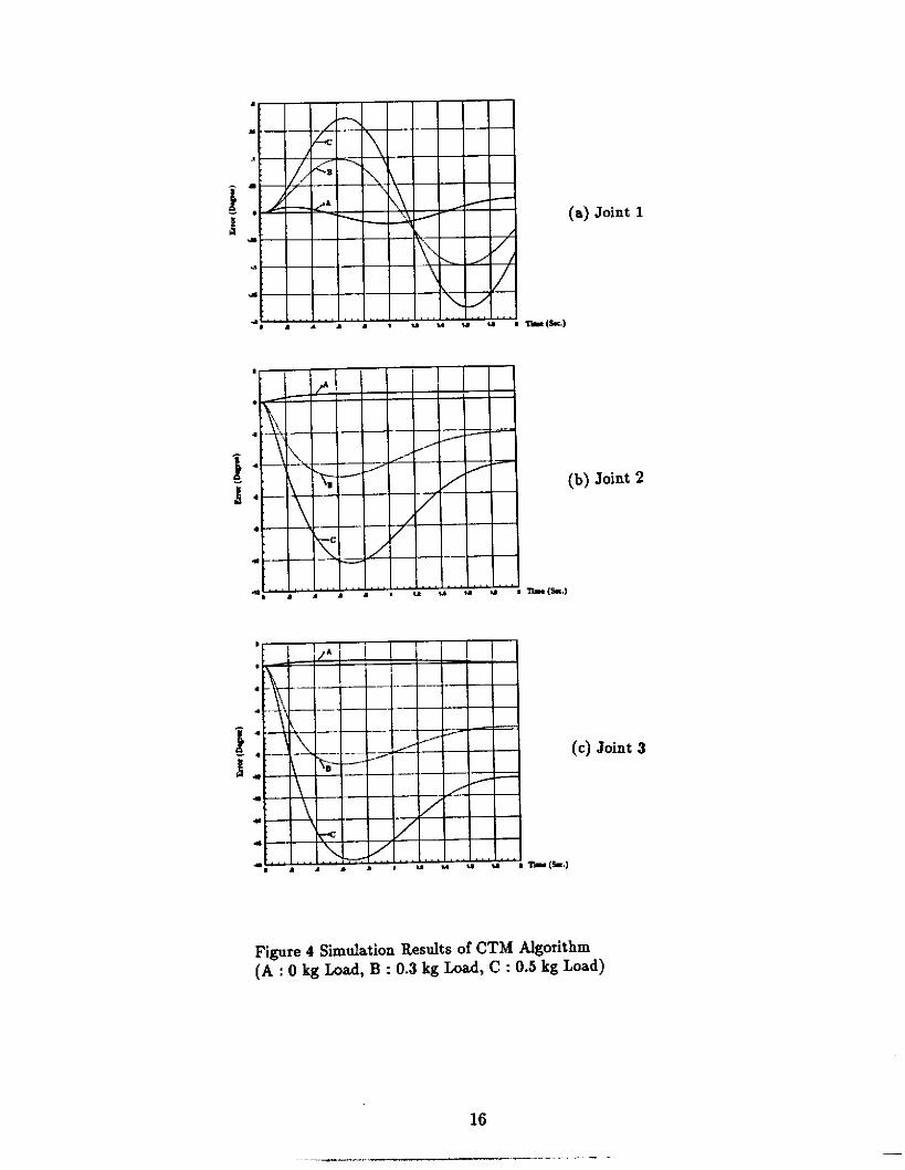
Figure 4 Simulation Results of CTM Algorithm (A : 0 kg Load, B : 0.3 kg Load, C : 0.5 kg Load)

Joint 1

Joint 3

Figure 5 Simulation Results of Theorem 1 (A : Load = 0 kg and Tp = 10ms, B : Load = 0.3 kg and Tp = C : Load = 0.5 kg and T,g = 50ms)

17

Joint 1

(a) Joint 2

T-* ( s 4

( e ) Joint 3

fh 1%)

Figure 6 Simulation Results of Theorem 2 (A : Load = 0 kg and Tp = 10m3, B : Load = 0.3 kg and Tp = 107713, C : Load = 0.5 kg and Tp = 50ms)

18

- -

For Comparison, the maximum absolute values, and the root-mean-square values of the errors and torques are summarized in Table XI.

Table II Slmulalion Results of the Proposed Algorkhms

When the payload is 0 kg and TO = 50 ms, the s u m of the root-mean-square values of three joint errors is 0.2747 (degree) using the CTM algorithm, while it is 0,0009 (degree) using the proposed algorithm. Both proposed two algorithms presented better performances than the CTM algorithm in the sense of the tracking errors. As the payload increases, the root-mean-square error is rapidly increased from 0.2747 (degree) to 4.4950 (degree) using the CTM algorithm, while using the proposed algorithms the resultant error maintains nearly unchanged. Especially, note that using the proposed algorithm the tracking error is not increased so much as the increase of the payload error, for the case Tp = 50 ms.

The simulation results have shown that by the proposed algorithms the input torque changed smoothly, which is desirable in the implementation. When the payload is 0.5 kg and Tp = 50 ms, the sum of the root-mean-square values of the three joint torques is 4.334 (N . rn) using the CTM algorithm, while it is 4.410 (N . rn) using the proposed algorithm. To compensate for the disturbance of the payload error, a slightly large input torque is necessary. For the proposed algorithms, the input torques with Tp = 50 ms are slightly larger than that in the case T p = 10 ms.

From the simulations, we have found that the proposed algorithm provides an excellent robust performance to the disturbance of the modeling error.

5 Conclusions In this report, a composite control algorithm for the control of robot manipulators is pro- posed. The discrete component is a nominal torque for the feedforward compensation for the nonlinear coupling torques between the links.

The feedback component uses the sliding mode control of the Variable Structure System which presents a stable performance. The proposed algorithm does not impose an additional computation on the real-time implementation, since the computation of model is necessary only for the feedforward component which can be computed off-line. In the digital implemen- tation, the controller takes the form of the multiple-rate structure. The feedback controller does not need much computational time and allows the short sampling time, and thus a fast motion of a multi-degree freedom robot manipulator can be executed by using a simple computer, or even a single board computer with an 8-bit CPU. Moreover, the time delay of the measurement can be negligible, since the measurement is utilized only in the feedback component.

The simulation results have shown the efficiency of the proposed algorithms for the tra- jectory tracking and the robust property to the modeling inaccuracy and unknown payloads.

Acknowledgements We wodd like to thank Professor Jong-Soo Lee for his work and helpful discussions through- out this work.

22

References [l] C.H.An, C.G.Atkinson, and J.M.Hollerbach. Experimental determination of the effect of

feedforward control on trajectory tracking errors. In P m . IEEE Int. Conf. on Robotics and Automation, pages 55-60, 1986.

[2] C.S.G.Lee, B.H.Lee, and R.Nigam. Development of the generalized d’alembert equations of motion for mechanical manipulators. In P m . IEEE 22nd Conf. Decision and Control, pages 1205-1210, 1983.

131 C.S.G.Lee and M.J.Chung. Adaptive perturbation control with feedforward compensa- tion for robot manipulators. J. ofDynamic Syst. Measumment and Control, Trans. on ASME, 106:134-142, 1984.

[4] F.Harashima, H.Hashimoto, and K.Maruyama. Practical robust control of robot arm using variable structure system. In Pmc. IEEE Int. Conf. on Robotics and Automation, pages 532-539, 1986.

[5] I.J.Ha and E.G.Gilbert. Robust tracking in nonlinear systems. IEEE Trans. on Auto- matic Control, AC-32:763-771, 1987.

[6] J.J.Slotine. The robust control of robot manipulators. In Int. J. of Robotics and Re- search, pages 49-64, 1985.

[7] J.N.Franklin. Matriz Theory. New Jersey : Prentice Hall, 1968.

[8] J.Y.Luh, M.W.Walker, and R.P.Pau1. On-line computational scheme for mechanical manipulators. Journal of Dynamic System Measurement and Control, Trans. on ASME, 102:69-76, 1980.

[9] K.G.Shin and X.Cui. Effects of computing time delay on real-time control systems. In Proc. American Control Conference, pages 1071-1076, 1988.

[lo] K.K.D.Young. Controller design for a manipulator using theory of variable structure systems. IEEE Tmns. on System Man and Cybernetics, SMC-8, 1978.

[ll] K.S.Fu, R.C. Gonzalez, and C.S.G. Lee. Robotics : Control, Sensing, Vision, and

I121 M.Brady, J.M.Hollerbach, T.L.Johnson, T.Lozano-Perez, and M.T.Mason. Robot Mo-

Intelligence. New York : Mcgraw-Hill, 1987.

tion : Planning and Control. Massachusetts : The MIT Press, 1982.

[13] 0.Egeland. On the robustness of computed torque method in manipulator control. In Proc. IEEE Int. Conf. on Robotics and Automution, pages 1203-1208, 1986.

[14] R.Bellman and F.Be&enba&. Inequalities. New York : Springer-Verlag, 1965.

[15] R.Nigam and C.S.G.Lee. A multiprocessor-based controller for the control of mechanical manipulators. IEEE Trans. on J . of Robotics and Automation, RA-1:173-182, 1985.

23

[16] T.Kailath. Linear System. New Jersey : Prentice Hall, 1980.

[17] V.D.Touraais and C.P.Neuman. Robust nonlinear feedback control for robotic manipu- lators. IEE Proceedings, Part 0, 132:134-143, 1985.

[IS] V.LUtkin. Sliding Modes and Their Application in Variable Structure Systems. Moscow , MIR Publisher (English Translation), 1978.

24