arX

iv:1

601.

0473

6v1

[st

at.A

P] 1

8 Ja

n 20

16

A Consistent Direct Method for Estimating Parameters

in Ordinary Differential Equations Models

Sarah E. HolteDivision of Public Health Sciences

Fred Hutchinson Cancer Research Center1100 Fairview Ave North, M2-B500

Seattle, WA 98109, USAemail: sholte@fhcrc.org

February 12, 2018

Abstract

Ordinary differential equations provide an attractive framework for modeling temporal dy-namics in a variety of scientific settings. We show how consistent estimation for parameters inODE models can be obtained by modifying a direct (non-iterative) least squares method similarto the direct methods originally developed by Himmelbau, Jones and Bischoff. Our method iscalled the bias-corrected least squares (BCLS) method since it is a modification of least squaresmethods known to be biased. Consistency of the BCLS method is established and simulationsare used to compare the BCLS method to other methods for parameter estimation in ODEmodels.

Keywords: Linear regression, longitudinal data, nonlinear regression, ordinary differential equa-

tions, parameter estimation.

1 Introduction

Ordinary differential equations (ODEs) have been used extensively in a wide variety of scientific

areas to describe time varying phenomena. Physicists have used equations of this type to understand

the motion of objects for centuries. ODE’s are used in nearly every field of engineering and chemists

use ODE models to evaluate chemical reactions. Ecologists have used ODE’s to understand the

dynamics of animal and plant populations [11], meteorologists have used them to understand and

predict patterns in the weather and atmosphere [20], and economists have used them to understand

and predict patterns in financial markets [37]. More recently, biologists and health scientists have

begun to use differential equations to make sense of observed nonlinear behaviors in their fields of

study. One area where the use of differential equations is well integrated with data analysis is the

evaluation of drug metabolism, the study of pharmacokinetics and pharmacodynamics (PK/PD).

1

Studies of how drugs are metabolized are part of the development of nearly all compounds available

for use in humans today. Reviews of the use of differential equations in both individual and

population level PK/PD include [3, 5, 6, 21, 29]. Software packages for parameter estimation

for population PK/PD models are available in both SAS [12] and Splus [31] . In other areas of

biology and clinical research, ordinary differential equation (ODE) models have been used as a tool

in exploring the etiology of HIV and Hepatitis B and C infections and the effects of therapy on

these diseases. In [15, 33, 23, 24] ordinary differential equations were used to analyze the temporal

dynamics of HIV viral load measurements in AIDS patients. The results had a tremendous scientific

impact, revealing that the HIV virus replicates rapidly and continuously, in spite of the prolonged

interval between infection and development of AIDS.

In some cases, ODE’s are used for theoretical purposes only; to provide “what if” scenarios

to be further studied by experimental scientists. However, more and more, ODE’s are used in

combination with observed data for parameter estimation and statistical inference of parameters

in ODE models. In most cases, the parameters of interest appear in a nonlinear form in the likeli-

hood or cost equation. Estimates are often obtained using standard nonlinear least squares (NLS)

estimation techniques. One drawback of the NLS estimation technique using conventional gradi-

ent based optimization methods such as Gauss-Newton or Levenberg-Marquart is the instability

of the procedure since estimates are obtained by an iterative numerical procedure ([25], Chapter

10). NLS procedures may fail to converge to global minima depending on the choice of starting

values for iteration, particularly if the least squares solution has multiple local minima or saddle

points. Global optimization methods are often available, however many analysts continue to rely

on algorithms such as nonlinear least squares that require a choice of starting values. Certain like-

lihood surfaces or cost functions may be exceptionally complex with ridges which tend to appear

near bifurcation values of the parameters in the ODE model. Furthermore, it is well known that

nonlinear regression estimates may be biased [2] when small samples are used for estimation.

When parameters in an ODE model appear linearly in the vector field which defines the ODE

system, it is possible to estimate the parameters either iteratively (e.g., nonlinear least squares)

or non-iteratively. In this paper we will use the term direct to refer to non-iterative methods.

Direct methods can be based on differentiation or integration and are generally combined with

a least squares estimation step. Direct methods based on integration were originally described

in [14] and are further developed in [1, 10, 16, 18]. In general, the ODEs are transformed into

integral equations and the integrals are approximated via methods of quadrature which yields

algebraic equations that can be solved for the approximate parameters using a linear least squares

2

approach. Differentiation methods are described in [1, 16, 30, 32] and involve constructing a cubic

spline using the observed data for each dependent variable. Values for the unknown parameters

are estimated using linear least squares, i.e., minimizing the differences between the derivatives of

the spline functions and corresponding model equations. Both the differentiation and integration

approaches result in linear least squares problems which can be solved without iteration. When

there is negligible measurement error and equally spaced values of the dependent variable, the two

approaches provide similar estimates [34]. In the case where these two assumptions are not met,

the integration approach is preferred over the differentiation approach [35]. Differentiation requires

differencing of observed data, an approach which is known to inflate errors in the data. In contrast,

integration involves sums of observed data; a smoothing approach which can reduce errors. An

approach which relies on integration allows estimation of the initial size of the states of the system

if these are not known.

There has been very little investigation of the statistical properties of parameter estimates in

ODE models obtained by direct methods, possibly since it is known that parameter estimates

obtained via these direct methods do not have optimal statistical properties [16]. Specifically, the

estimates are not unbiased, efficient, or consistent. While these early direct methods did not have

optimal statistical properties it is possible that adjustments can be identified so that the resulting

direct method has desirable statistical features.

Recently, Liang and Wu [19] describe a direct method based on differentiation, local smoothing

of the data and linear least squares regression of correlated quantities, which they refer to as pseudo-

least squares (PsLS) method. They show that under reasonably general conditions their PsLS

estimate of parameters in an ODE model is consistent with an asymptotically normal distribution.

However, choice of bandwidth for the kernel smoothing required by this method is critical and

may require further research in order to provide the most accurate and efficient results. Ramsey

and colleagues [27, 28] have used functional estimation or principle differential analysis (PDA)

approaches to replace state variables with their (smoothed) estimates, and proceed with estimation

of parameters using estimated values of the solutions to the system of ODEs. These methods, like

those of Liang and Wu, use differentiation rather than integration.

In this paper we introduce a direct algorithm similar to those developed by or based on the

work of Himmelbau, Jones and Bischoff [14]. Our approach incorporates a bias correction factor so

that the method is consistent, and does not require smoothing or functional estimation. As such it

retains the simplicity of early direct methods [1, 18, 10, 14, 16, 30, 32] but has many of the desirable

statistical properties of the more recently developed direct methods [19, 28]. Our method relies on

3

integration similar to the methods described in [1, 10, 14, 16, 18]. We refer to the proposed method

as the bias-corrected least squares method (BCLS) and the focus of this paper is to evaluate the

statistical properties of the estimates produced by the BCLS method. Since the BCLS method

relies on integration rather than differentiation, estimation of the initial states of the system in

addition to parameters appearing linearly in the system is possible. The method is applied to two

examples and its properties contrasted with those of the NLS and PsLS methods with simulation

studies. A proof of the consistency of the method is provided in the appendix.

2 The Bias-Corrected Least Squares Method

2.1 Mathematical and Statistical Model Specification

The bias-corrected least squares method applies to data, y(t), on observations with time varying

expectation given by the solutions of system of q = 1, · · · , s ODEs, observed at t = (t0, · · · , tn), n

observation times. It is not necessary that all s compartments be sampled at the same times, but

for ease of notation it is assumed that this is the case in this work. The statistical and mathematical

model assumptions for the the data y(t) with distribution Y(t) are summarized as follows:

(A.1) : Specification of the mean structure via a mathematical model

– There exists a vector of functions X(t) = {X1(t), · · · ,Xs(t)} which satisfies the system

of differential equations:

dXq

dt=

mq∑

k=1

βq,khq,k(X1, · · · ,Xs), Xq(t0) = Xq,0, q = 1, · · · , s (1)

such that that the expectation, E{Y(t)} is equal to X(t).

(A.2) : Specification of variance/covariance structure

– Yq(t) = Xq(t) + ǫq, ǫq ∼ (0,Σq), q = 1, · · · , s.

– Σq is a diagonal matrix with constant diagonal entries σq, q = 1, · · · , s.

– ǫr and ǫq are independent for all 1 ≤ r < q ≤ s.

– var(Yi) and var{hq,k(Yi)} are bounded by a common bound B for all i, q, and k.

(A.3) : Data sampling requirements

– The maximum interval length defined by the sampling times is O(n−1).

4

– At least one of the compartments is not in equilibrium throughout the entire time course

of data collection .

The values βq,k and in some cases the initial conditions Xq,0 are parameters that will be esti-

mated from the data. The functions, hq,k, are any (linear or nonlinear) continuous functions of the

states of the system, which together with the parameters, βq,k, and initial conditions, Xq,0, define

the vector field of the differential equations relating the states X to their time derivatives. For the

qth state, the value mq is the number of terms in the expression which specifiesdXq

dt . Note that

the vector field defining the system of differential equations can be nonlinear in the states, i.e.,

hq,k(X) is not necessarily linear in the states, but must be linear in the parameters in order for the

bias-corrected least squares method (or any direct least squares based method) to be applicable.

Thus the BCLS method applies to a wide variety of nonlinear systems of ODE’s.

Condition (A.1) provides the relationship between the time-varying expectation of the data and

a system of ODEs. Condition (A.2) requires that conditional on the expected value, observations

from different compartments of the system of ODE’s are independent. This requirement is not

overly restrictive, since the use of ODE’s is intended to capture the relationships between the

observed compartments. Condition (A.2) also specifies that the variance of observations from

different compartments can differ. The second part of condition (A.3) is included to prevent non-

identifiability, but does not insure identifiability of the estimation procedure.

The key component of the BCLS method is the use of bias correction functions which are

needed to account for bias which is introduced when making nonlinear transformations of random

variables. These bias correction functions are used as weights in the least squares estimation. These

functions can be defined in a number of ways. For a function h = hq,k, identify the difference,

E[h{Y (t)}]− h{E[Y (t)]} and then subtract it from h to define h⋆ as follows:

h⋆{Y (t)} = h{Y (t)} − (E[h{Y (t)}] − h{E[Y (t)]}) . (2)

An alternative is to define h⋆ as:

h⋆{Y (t)} = h{Y (t)}h{E[Y (t)]}

E[h{Y (t)}](3)

Taking expectations of both sides of (2) or (3) shows that either definition satisfies

E[h⋆q,k{Y(t)}] = hq,k{X(t)}, q = 1, · · · , s, k = 1, · · · ,mq. (4)

Any function, h⋆ which satisfies (4) can be used to weight the linear regression step of the estimation

procedure to eliminate bias in the resulting point estimates. The previous two examples show that

5

such a function always exists; the most efficient form of h⋆ for a specific model generally depends

on the error structure of the data (e.g additive vs multiplicative).

The following notation will be used: Let yq,i, q = 1, · · · , s, i = 1, · · · , n, denote an observation

with expectation given by Xq in Eq. (1) at time ti; yq(t) denote the vector of all observations

from the qth compartment, Xq(t); y(ti) denote the vector of observations on all compartments at a

single observation time, ti; and y(t) denote the matrix of observations on all compartments at all

observation times. In general, lower case letters represent observed data, and upper case represent

the associated random variables or state variables of the system of ODE’s. In the following sections,

when direct estimation of parameters in an ODE model is performed without the bias-correction

we will refer to the resulting point estimates as simply least squares (LS) estimates or least squares

without bias correction.

2.2 Estimation Algorithm

The BCLS method is designed to simplify a nonlinear regression problem by reducing it to a linear

regression problem. This is achieved by transforming the system of differential equations (1) into

a system of integral equations and treating the transformed system as a statistical model for a

collection of linear regressions with covariates which approximate the integrals. Approximations

to these covariates are obtained using the observed data. Specifically, Eq. (1) is equivalent to the

system of integral equations:

Xq(t) =

mq∑

k=1

βq,k

∫ t

t0

hq,k{X(τ)}dτ +Xq,0 q = 1, · · · , s.

so that (A.1) implies

E{Yq(t)} =

mq∑

k=1

βq,k

∫ t

t0

hq,k{X(τ)}dτ +Xq,0 q = 1, · · · , s. (5)

The expectations in Eq. (5) suggest s linear regression models with response variables (out-

comes) yq(t) and covariates which approximate the integrals∫ tt0hq,k{X(τ)}dτ , k = 1, · · · ,mq,

q = 1, · · · , s. If an intercept is included in the regression model it provides an estimate for the

initial condition, Xq(t0), and the estimated coefficients of the covariates provide estimates of the

parameters βq,1, · · · , βq,mq. If the initial value yq(t0) is known, the response variable can be defined

as yq(t)− yq(t0) and linear regression without intercept can be used. For ease of notation, we now

drop the subscript q in the response variable and describe each of the s states separately.

To obtain covariates for the regression analysis, any method of integral approximation can

be used. For the examples and simulations in this manuscript, the trapezoid method is used to

6

approximate the integrals∫ ti0 hk{X(τ)}dτ and construct covariates, zk(ti), defined by: zk(t0) = 0

and for k = 1, · · · ,m and i = 0, · · · , n,

zk(ti) =

i∑

j=1

[h⋆k{y(tj−1)}+ h⋆k{y(tj)}] ∗ (tj − tj−1)

2

where h⋆k is the bias correction adjustment which satisfies (4), e.g (2) or (3). Let zk(t) denote

the vector, {zk(t0), · · · , zk(tn)}, and z(t) denote the matrix with columns zk(t), k = 1, · · · ,m.

Although the trapezoid rule for integral approximations is used for the examples and simulations

presented in this work, many methods are available for integral approximation ([25], Chapter 4).

The most simple integral approximation is defined by using only the left endpoints of the intervals

and can be described using the observed data as follows:

zk(ti) =∑

j<i

h⋆k{y(tj−1)} ∗ (tj − tj−1)

Note that if only the left hand endpoint is used in the definition of zk(t), the covariates are

independent of the corresponding response, since the definition of zk(ti) depends only on data

observed at time points t0, · · · , ti−1 and the ith response is the data observed at time ti. Although we

use this simple approximation to demonstrate consistency (Appendix 1), in practice the trapezoid

rule produces more accurate estimates.

We can now define the linear regression model as

Y (t) = Z(t) β + ǫ, ǫ ∼ (0,Σ2)

where Σ2 is the variance/covariance matrix for the residual errors. If only the left hand endpoint

of each interval is used in the definition of zk(t), Condition (A.2) guarantees that Σ is a diagonal

matrix, although the variances associated with each state are not assumed to be the same for all

states. In this work, we assume that Σ is known or will be obtained using an independent method.

These variances are usually needed to construct the bias correction functions, h⋆k.

To estimate β, linear regression with response y(t) ( or y(t)− y(t0) ) and the covariate matrix

z(t) is performed so that

β = (z(t)′z(t))−1z(t)′y(t) (6)

In [19], the authors refer to regression analysis of this type as pseudo-least squares, (PsLS) since the

minimization that occurs with the linear regression algorithm is not minimizing a true likelihood.

The same is true of bias-corrected least squares.

To demonstrate consistency of the BCLS method we rely on the following Theorem.

7

Theorem 1. Assume conditions (A.1)-(A.3) (from Section 2.1 ) are satisfied and that βnis the unique root

of the estimating function, defined by Un(β) =1

n

n∑

i=1

zT

i{y

i− ziβ} = 0 . Then:

I Un(βn) is a consistent estimator of zero.

II E{ 1

n

∑n

i=1ZT

iZi} is bounded and non-zero.

III var{ 1

n

∑n

i=1ZT

iZi} → 0 as n → ∞.

Thus, the linear least squares estimate, β = (z(t)′

z(t))−1z(t)′

y(t) is a consistent estimator of β.

The final conclusion, that the three conditions listed in Theorem 1 imply consistency of estimator

β from standard linear regression follows from results in [4]. The key technical issue is that the

derived covariates, z(t), are functions of the observed data rather than of the state means and

are therefore measured with error, and that the covariates themselves are correlated with each

other. However, contrary to the classical measurement error setting the variance of the covariates

is O(n−1) and therefore bias due to error in the covariates is asymptotically eliminated. It will be

shown in the appendix that the BCLS method satisfies condition [I-III].

3 Example: A single compartment nonlinear ODE

3.1 Data Analysis: Growth colonies of paramecium aurelium

To illustrate the method using a model defined by a nonlinear differential equation with a single

compartment, data on the growth of four colonies of the unicellular organism, paramecium aurelium,

were analyzed. These data are described in [7, 13]. In this example a differential equation represents

the size of the population of the colony of paramecium over time. We assume that the data on

colony size, y(t), follows a log-normal distribution, with

log{Y (t)} = log{X(t)} + ǫ, ǫ ∼ i.i.d. N(0, σ2)

where X(t) satisfies the standard logistic growth curve described by the nonlinear differential equa-

tion

dX

dt= X(a− bX), X(0) = y0 (7)

The parameter a is the growth rate per capita, ab is the carrying capacity of the population, and

y0 is the initial size of the populations which is known by design; y0 = 2 in all four data sets. A

log transform is applied to the data for analysis and parameter estimation so that a log-transform

of the differential equation (7) is required.

d{log(X)}

dt= a− bX, log{X(0)} = log(y0). (8)

8

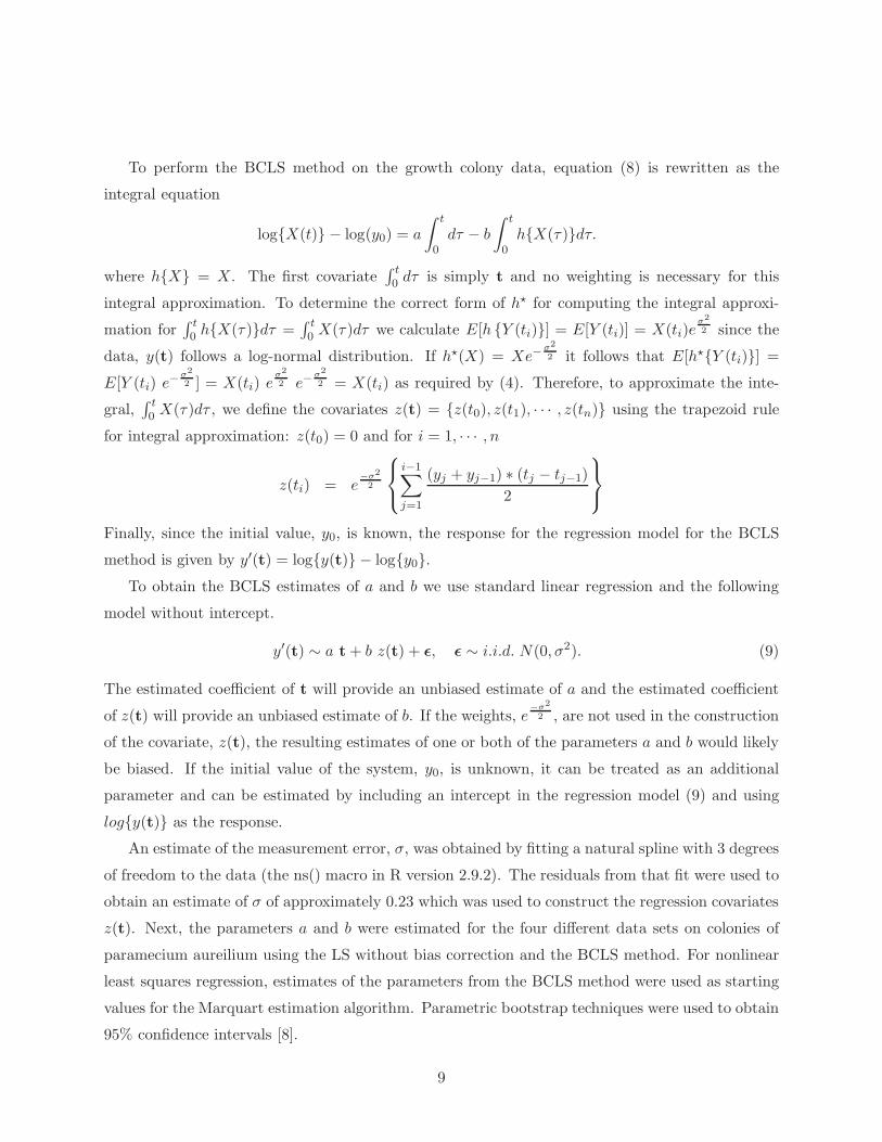
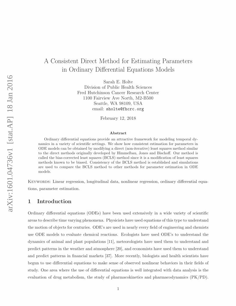
To perform the BCLS method on the growth colony data, equation (8) is rewritten as the

integral equation

log{X(t)} − log(y0) = a

∫ t

0dτ − b

∫ t

0h{X(τ)}dτ.

where h{X} = X. The first covariate∫ t0 dτ is simply t and no weighting is necessary for this

integral approximation. To determine the correct form of h⋆ for computing the integral approxi-

mation for∫ t0 h{X(τ)}dτ =

∫ t0 X(τ)dτ we calculate E[h {Y (ti)}] = E[Y (ti)] = X(ti)e

σ2

2 since the

data, y(t) follows a log-normal distribution. If h⋆(X) = Xe−σ2

2 it follows that E[h⋆{Y (ti)}] =

E[Y (ti) e−σ2

2 ] = X(ti) eσ2

2 e−σ2

2 = X(ti) as required by (4). Therefore, to approximate the inte-

gral,∫ t0 X(τ)dτ , we define the covariates z(t) = {z(t0), z(t1), · · · , z(tn)} using the trapezoid rule

for integral approximation: z(t0) = 0 and for i = 1, · · · , n

z(ti) = e−σ2

2

i−1∑

j=1

(yj + yj−1) ∗ (tj − tj−1)

2

Finally, since the initial value, y0, is known, the response for the regression model for the BCLS

method is given by y′(t) = log{y(t)} − log{y0}.

To obtain the BCLS estimates of a and b we use standard linear regression and the following

model without intercept.

y′(t) ∼ a t+ b z(t) + ǫ, ǫ ∼ i.i.d. N(0, σ2). (9)

The estimated coefficient of t will provide an unbiased estimate of a and the estimated coefficient

of z(t) will provide an unbiased estimate of b. If the weights, e−σ2

2 , are not used in the construction

of the covariate, z(t), the resulting estimates of one or both of the parameters a and b would likely

be biased. If the initial value of the system, y0, is unknown, it can be treated as an additional

parameter and can be estimated by including an intercept in the regression model (9) and using

log{y(t)} as the response.

An estimate of the measurement error, σ, was obtained by fitting a natural spline with 3 degrees

of freedom to the data (the ns() macro in R version 2.9.2). The residuals from that fit were used to

obtain an estimate of σ of approximately 0.23 which was used to construct the regression covariates

z(t). Next, the parameters a and b were estimated for the four different data sets on colonies of

paramecium aureilium using the LS without bias correction and the BCLS method. For nonlinear

least squares regression, estimates of the parameters from the BCLS method were used as starting

values for the Marquart estimation algorithm. Parametric bootstrap techniques were used to obtain

95% confidence intervals [8].

9

The estimated values of a and b and their 95% parametric bootstrap confidence intervals are

shown in Table 1. Non-parametric bootstrap confidence intervals were also obtained for the BCLS

method, since non-parametric bootstrap does not require an analytic or numerical solution to

equation (7). The data sets and fitted trajectories from both the NLS and BCLS estimation

procedures are shown in Figure 1. The estimates and confidence intervals obtained from the

two methods are quite similar, and Figure 1 suggests that both methods produce estimates of

the underlying trajectories which fit the data well. For these four data sets, the BCLS method

produced virtually the same results as the LS method without bias correction (results not shown).

3.2 Simulations

To compare the BCLS method to NLS and the PsLS method described in [19] for accuracy and

efficiency we simulated data from the statistical model

log{Y (t)} = log{X(t)} + ǫ, ǫ ∼ i.i.d N(0, σ2)

where X(t) is the solution of equation (7) with parameters set as follows: a = 0.8, b = 0.0015, and

y0 = 2. These parameters were chosen based on the fits to the four data sets shown in Table 1. A

range of values for residual error, σ, were evaluated in order to demonstrate the increase in bias in

the estimate of the parameter b using LS without adjusting the covariate z(t) as described in the

previous section. Two sets of observations times were evaluated; Each consisted of observation times

between t = 0 and t = 20. The first set of observation times consisted of 21 total observations,

evenly spaced 1 unit apart between 0 and 20. The second set of observation times consisted of

201 total observations, evenly spaced 0.1 units apart between 0 and 20. Individual simulations

we conducted for each of the two sets of observation times and each of the following values of σ,

(0.2, 0.4, 0.6, 0.8) for a total of 8 simulation studies.

For each combination of observation times and values of σ, the data were simulated 1000

times and the BCLS, LS (without weights to adjust for bias), PsLS and NLS estimates of a and

b were used to estimate model parameters. To evaluate the PsLS method the local polynomial

smoothing macro locpoly() from the R KernSmooth package was used to obtain the smoothed

state and derivative curves. A bandwidth of order log(nt)−1/10 ∗ nt−2/7 was chosen for both state

and derviative estimation as suggested in [19], where nt is the sample size in each simulation. A

number of other choices for bandwidth we considered, including the standard choice of order nt−1/5.

The choice of bandwidth used in the simulations was made based on selecting the bandwidth that

produced the least biased estimates.

10

Figure 2 depicts the estimated values of the parameters a and b using the LS method (dotted

lines), the BCLS method (combined dash and dotted lines), the NLS method (solid line) and the

PsLS method (dashed line). No bias correction is necessary for the integral approximation of the

covariate used to estimate the parameter a so that bias-corrected and unadjusted least squares

estimates of a are identical. Panels A and B of Figure 2 show how bias in the estimated parameters

varies with measurement error in the simulated data when 21 equally spaced time points between

t = 0 and t = 20 are used; Panels C and D depict the same when the sample size is increased to

201 time points. The Monte Carlo means and standard errors for the estimated parameters from

each of the simulations with 21 equally spaced observations are shown in Table 2.

As expected, Figure 2, panels B and D show that bias increases in the LS estimate of the

parameter b as simulated measurement error, σ, increases from 0.2 to 0.8 when bias correction

is not used in covariate definition. Also as expected, the bias in the LS estimate of b without

bias-correction is essentially unaffected by sample size (Figure 2, Panels C and D). With a total

of 21 time points, the BCLS method appears to underestimate the parameter a slightly, likely due

to errors in integral approximation of a convex function with relatively sparse measurements. The

NLS method appears to overestimate that same parameter, probably due to the bias associated

with nonlinear regression [2]. The bias in the BCLS and NLS estimates decreases substantially

when sample size is increased to 201 timepoints(Panes C and D). Figure 2 also shows that bias

in PsLS estimates of both a and b changes as σ increases, indicating the constant in the choice of

bandwidth affect bias in parameters estimated using this method. . An increase in sample size

from 21 time points to 201 time points reduces the bias in the estimate of the parameter a from

the strongly consistent PsLS method [19], however, bias in the estimate of parameter b seems to

shift but not decrease, possibly due to an improper choice of bandwidth. Additional simulations

with larger samples sizes showed this bias decreases but not until an extremely large sample size

is used. The numeric results from the simulation studies with 21 observation points are shown in

Table 2 and confirm the findings described for Figure 2.

The efficiency of the four methods can be evaluated using the Monte Carlo standard errors

shown in Table 2. These standard errors indicate that the variability of the estimation procedures

are quite similar, with the NLS method providing slightly more precise (lower standard error)

estimates. This is expected, since in this setting, NLS is the maximum likelihood method for

parameter estimation. In general, the Monte Carlo standard errors for estimates obtained with the

PsLS method are slightly larger than those obtained with BCLS, possibly due to differencing of the

data required by methods which rely on differentiation. The Monte Carlo standard errors from all

11

three methods for the simulations with 201 equally spaced time points between t = 0 and t = 20

are show a similar pattern in standard errors from the three methods. (Results not shown).

4 Example 2: Nonlinear System of ODEs with two compartments

The Fitzhugh-Nagumo system of differential equations [9, 22] is a simplified version of the the well

known Hodgkin-Hukley model [17] for the behavior of spike potentials in the giant axon of squid

neurons. The equations

dV

dt= C(V −

V 3

3+R), V (0) = v(0) (10)

dR

dt= −

1

C(V − a+ bR), R(0) = r(0) (11)

describe the reciprocal dependencies of the voltage compartment V across an axon membrane and

a recovery compartment R summarizing outward currents. Solutions to this system of differential

equations quickly converge for a range of starting values to periodic behavior that alternates between

smooth evolution and sharp changes (bifurcations) in direction. These solutions exhibit features

common to elements of biological neural networks [36]. The system has been used by a number

of authors including [28, 19] to demonstrate methods of parameter estimation for data with time

varying expectation given by this system of differential equations.

For this example there are two random variables: the voltage across an axon membrane, Y1(t),

and a recovery measurement of outward currents, Y2(t). We assume that observed data, y1(t) and

y2(t) follow independent normal distributions with

Y1(t) = V (t) + ǫ1, ǫ1 ∼ i.i.d. N(0, σ21) (12)

Y2(t) = R(t) + ǫ2, ǫ2 ∼ i.i.d. N(0, σ22) (13)

where V (t) and R(t) satisfy the differential equations (10) and (11).

The likelihood surface for data with expectation given by a nonlinear system of differential

equations may be extremely complex and can contain multiple local maxima (equivalently, local

minimum solutions to the nonlinear least squares regression model). For the Fitzhugh-Nagumo

equations we considered two sets of parameters; C = 3, a = 0.58, b = 0.58 and C = 3, a = 0.34,

b = 0.20. The parameters C = 3, a = 0.58, b = 0.58 are very near a supercritical Hopf bifurcation

value of the system; from a stable steady state to an oscillating limit cycle. There is a dramatic

change in the least squares surface as the parameters a and b vary about 0.58 (with C = 3 fixed).

Contours of the least squares surface for a set of zero noise data are shown in Figure 3 panels A,

12

B, and C. Panel A shows the contours of the least square surface for a range of a = 0.4 to 1.4 and

b = 0 to 0.2 to 2.2. The blue box contains the true solution, a = 0.58 and b = 0.58, the red box

contains a local minimum. Panels B and C show close ups of the red and blue regions, respectively.

Panel B suggests that there is local minimum in the least squares fit surface at approximately a

= 1.5, b = 2.0. Panel C suggests that the least squares fit surface is badly behaved near the true

solution, with a long ridge containing the true solution, which is near a bifurcation values for the

parameters a and b.

Figure 3 Panels D,E, and F show similar regions of a least squares surface for zero noise obser-

vations from the Fitzhugh-Nagumo system with parameters C = 3, a = 0.34, and b = 0.2. This

system has a local minimum shown in the red square and the true solutions shown in the blue

square Panel D. Close-ups of these regions are shown in panels E and F respectively. For this

collection of parameters, the least squares surface near the true solution is well behaved (Panel F),

however, a local minimum in the surface exists near a = 1.7, b =2.8 (Panel E).

4.1 Simulations

To compare the BCLS method to NLS and PsLS for accuracy and efficiency in estimating param-

eters in the Fitzhugh-Nagumo model, data was simulated from the statistical model (12) and (13),

for two sets of parameter values; C =3, a = 0.34, b = 0.2 and C =3, a = 0.58, b = 0.58. For each

of the two sets of parameter values, a range of residual standard errors σ1 and σ2 were evaluted ;

σ1 = 0.05, 0.1, and 0.15, and σ2 = 0.05, 0.1, and 0.15. Time points evenly spaced time points at

intervals of 0.1 between 0 and 20 for a total of 201 time points were considered. Initial conditions

for the system, v0 = -1 and r0 =1 were used for all simulations. The data were simulated 1000

times for each set of parameter values and values of σ1 and σ2. All three parameters C, a, and b as

well as the initial conditions, v0 and r0 were estimated using nonlinear least squares, bias-corrected

least squares and least square without bias correction. Since PsLS relies on derivatives rather than

integrals, estimation of the intial conditions v0 and r0 is not possible, so that only estimates of the

three model parameters, a, b and C were obtained using the PsLS method.

For each of the 1000 replicates, nonlinear least squares regression of all five values is conducted

simultaneously using simulated data y1(t) and y2(t) and solutions to (10) and (11) to form the

weighted (when σ21 6= σ2

2) least squares expression

n∑

i=1

(y1(ti)− V (ti))2

σ21

+(y2(ti)−R(ti))

2

σ22

.

The BCLS estimation is conducted in two steps. First,the parameter C and initial condition v0

13

are estimated using data y1(t) a regression model based on (10). Next the parameters a and b

and initial condition r0 are estimated using data y2(t), a regression model based on (11), and the

estimate of C obtained in the first step.

To estimate C and v0, equation (10) is re-written as the integral equation

V (t) = C

∫ t

0h1,1(V,R)dτ + v0 (14)

where h1,1(V,R) = V − V 3

3 +R. Since E[Y 31 ] 6= E[Y1]

3 a bias correction function must be identified.

Calculating E[Y1 −Y 31

3 + Y2] = V + (V3

3 + 3V σ21) +R, it is clear that

h⋆1,1(V,R) = V −V 3

3+R− 3V σ2

1

satisfies condition 4. Therefore, to approximate the integral in (14) we define the covariates z(t) =

{z(t0), z(t1), · · · , z(tn)} using the trapezoid rule for integral approximation: z(t0) = 0 and for

i = 1, · · · , n

z(ti) =i∑

j=1

(h⋆1,1 [y1(tj), y2(tj)] + h⋆1,1 [y1(tj−1), y2(tj−1)]

)∗ (tj − tj−1)

2

Finally, since the initial value, v0, will be estimated, the response for the regression model for the

BCLS method estimates of v0 and C is given by y′(t) = y1(t). To obtain the integrated-data

estimates of v0 and C we fit a linear regression model with intercept based on

y′(t) ∼ v0 1+ C z(t) + ǫ1, ǫ1 ∼ i.i.d. N(0, σ21). (15)

The estimated coefficient of z(t) will provide an unbiased estimate of C, denoted by C and the

e stimated intercept will provide an unbiased estimated of v0. When h1,1 is used to create the

covariates, rather than h⋆1,1, biased estimates of C and v0 are expected.

Using the estimated value C the BCLS method estimates of a, b and r0 are obtained by first

transforming (11) to the integral equation

C R(t) +

∫ t

0V (τ)dτ = r0 + at− b

∫ t

0R(τ)dτ. (16)

In this case integral approximations using the observed data are required to define both the response

and a covariate for the linear regression model that will be used to estimate a, b and r0. The

response for the linear regression model approximates the left-hand side of (16) and is denoted by

y′(t) = {y′(t0), y′(t1), · · · , y

′(tn)} where y′(ti) is defined as y′(t0) = Cy2(t0) and for i = 1, · · · , n:

y′(ti) = C y2(ti)) +

i∑

j=1

[y1(tj) + y1(tj−1)] ∗ (tj − tj−1)

2.

14

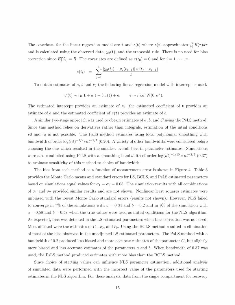
The covariates for the linear regression model are t and z(t) where z(t) approximates∫ t0 R(τ)dτ

and is calculated using the observed data, y2(t), and the trapezoid rule. There is no need for bias

correction since E[Y2] = R. The covariates are defined as z(t0) = 0 and for i = 1, · · · , n

z(ti) =

i∑

j=1

[y2(tj) + y2(tj−1)] ∗ (tj − tj−1)

2

To obtain estimates of a, b and r0 the following linear regression model with intercept is used.

y′(t) ∼ r0 1+ a t− b z(t) + ǫ, ǫ ∼ i.i.d. N(0, σ2).

The estimated intercept provides an estimate of r0, the estimated coefficient of t provides an

estimate of a and the estimated coefficient of z(t) provides an estimate of b.

A similar two-stage approach was used to obtain estimates of a, b, and C using the PsLS method.

Since this method relies on derivatives rather than integrals, estimation of the intial conditions

v0 and r0 is not possible. The PsLS method estimates using local polynomial smoothing with

bandwidth of order log(nt)−1/2∗nt−2/7 (0.20). A variety of other bandwidths were considered before

choosing the one which resulted in the smallest overall bias in parameter estimates. Simulations

were also conducted using PsLS with a smoothing bandwidth of order log(nt)−1/10 ∗ nt−2/7 (0.37)

to evaluate sensitivity of this method to choice of bandwidth.

The bias from each method as a function of measurement error is shown in Figure 4. Table 3

provides the Monte Carlo means and standard errors for LS, BCLS, and PsLS estimated parameters

based on simulations equal values for σ1 = σ2 = 0.05. The simulation results with all combinations

of σ1 and σ2 provided similar results and are not shown. Nonlinear least squares estimates were

unbiased with the lowest Monte Carlo standard errors (results not shown). However, NLS failed

to converge in 7% of the simulations with a = 0.34 and b = 0.2 and in 9% of the simulation with

a = 0.58 and b = 0.58 when the true values were used as initial conditions for the NLS algorithm.

As expected, bias was detected in the LS estimated parameters when bias correction was not used.

Most affected were the estimates of C , v0, and r0. Using the BCLS method resulted in elimination

of most of the bias observed in the unadjusted LS estimated parameters. The PsLS method with a

bandwidth of 0.2 produced less biased and more accurate estimates of the parameter C, but slightly

more biased and less accurate estimates of the parameters a and b. When bandwidth of 0.37 was

used, the PsLS method produced estimates with more bias than the BCLS method.

Since choice of starting values can influence NLS parameter estimation, additional analysis

of simulated data were performed with the incorrect value of the parameters used for starting

estimates in the NLS algorithm. For these analysis, data from the single compartment for recovery

15

of outward current, Y2(t), were used as outcomes in the nonlinear least square regression analysis

and only the parameters a and b estimated. The results of these analysis for simulated data with

201 equally spaced time points and residual standard error, σ2 = 0.05 are shown in Table 4 for the

model with a = 0.34 and b = 0.2 (first 3 columns) and for the model with a = 0.58 and b = 0.58

(last 3 columns). The values a = 0.4, 0.8, and 1.2 and b = 0.4 and 0.8 were used as starting values

for the NLS algorithm. The BCLS estimates of a and b were also used as starting values for the

NLS algorithm.

In most cases, when the incorrect values of the parameters were used as starting values for

NLS regression, the algorithm failed to converge, and when convergence occurred, the estimated

values of the parameters were incorrect. For example, with the true value of a = 0.34 and b = 0.2

if starting values of a = 0.8 or a = 1.2 is used (with either b = 0.4 or b = 0.8) the algorithm

converged for approximately 35% of the simulation replicates. When the algorithm did converge,

the Monte Carlo average of the estimate of a is approximately 1.72 and the average estimate of

b is approximately 2.77. These values correspond the local minimum of the least squares surface

shown in Figure 3 Panel E. Similarly, when the true value of a and b are both 0.58, for most

of the incorrect starting estimates, the NLS algorithm converged less for less than 35% of the

simulations The Monte Carlo average of the estimate of a when the NLS algorithm did converge to

the wrong value is approximately 1.15 and the average estimate of b is approximately 2.02 which

corresponds to the local minimum in the least squares surface for those parameters (Figure 3 Panel

B). When BCLS method was used to obtain starting values for the NLS regression algorithm,

unbiased estimates of both a and b are obtained, and the NLS algorithm converged for more than

90% of the simulation replicates.

5 Discussion

The bias-corrected least squares method is a computationally simple, non-iterative, and easily

implemented method for estimation of parameters in ODE models. It’s development and the

associated proof of consistency of the resulting parameter estimates illustrates that direct methods

(non-iterative) can be modified to so that the resulting estimator has desirable statistical properties.

The BCLS method retains the simplicity of early direct methods and has most of the desirable

statistical properties of more recently developed direct methods. A key advantage of the BCLS

method (and all direct methods) is that it does not require starting values for the estimation

algorithm; in fact, it can provide starting values for nonlinear least squares regression if desired.

Furthermore, it does not require choice of smoothing bandwidth of functional data analysis methods.

16

Since the BCLS method is based on integration rather than differentiation it can be used to estimate

initial states of the ODE model states in addition to ODE model parameters. This is not true of

direct methods which rely on differentiation such as PsLS.

The analysis and simulations described in Section 3 based on the population growth of parame-

cium aurelium show that the BCLS method performs comparably with the NLS method. In the

simulation studies conducted using the logistic growth equation, the BCLS method produces es-

timates that are often less biased than the recently developed PsLS method, a direct method

which uses differentiation and smoothing instead of integration. The bias observed in the PsLS

method is likely a result of the choice of bandwidth in the smoothing step; the use of integration

in the BCLS method alleviates the need for any smoothing of the data since integration itself is

a smoothing procedure. However, the bias due to integral approximations required by the BCLS

can be expected when the data are not densely sampled. The simulation studies conducted with

the Fitzhugh Nagamu equations in Section 4 provide further evidence that the BCLS method is a

viable alternative to NLS or PsLS regression. Those simulations demonstrate that the use of the

BCLS method to obtain starting values for NLS regression can reduce problems with convergence

and accuracy associated with the choice of starting values in the NLS method, especially in settings

with an exceptionally complex likelihood surface or cost function with multiple minima. These sim-

ulations also show that while the PsLS method has the capacity to produce less biased and more

accurate estimates for some parameters, these estimates rely heavily on the choice of bandwidth.

Furthermore, since BCLS is based on integration and PsLS is based on differentiation, the BCLS

method is able to provide estimates of the initial states of a system of ODE’s. This not possible

with the PsLS method. While both the BCLS method and the PsLS method are asymptotically

unbiased, the simulations in this paper suggest that the BCLS method has better small sample

properties if an optimal bandwidth is not used with PsLS. Furthermore, simulations suggest that

a bandwidth which produces the least bias in one estimated parameter may not be the optimal

choice for all parameters in the system.

There are a number of drawbacks to the BCLS method. In order to obtain unbiased parameter

estimates a separate analysis may be needed to obtain estimates of residual errors to be used in the

bias correction functions. Although the linear regression algorithm is used to obtain point estimates

for the parameters, this approach is not likelihood based so regression techniques for conducting

inference or obtaining confidence intervals cannot be used directly. However, bootstrapping tech-

niques are available to obtain confidence intervals for the estimated parameters. Another drawback

to the BCLS method is the assumption that parameters must appear linearly in the ODE system

17

(A.1). This excludes estimation of certain parameters in models such as the Michaelis-Menten

model for enzyme kinetics or saturating growth models for population dynamics. Nonlinear esti-

mation techniques could be used when parameters appear nonlinearly in the equations motivated

by Eq (5), and may offer improvements over directly solving the ODE and applying nonlinear es-

timation techniques to the resulting solution. This is an approach that was not considered in this

work. However, when known parameter appears nonlinearly in the system of ODEs it can be used

to create the covariates (or response) for the bias-corrected least squares method as demonstrated

in the estimation of a and b in the Fitzhugh-Nagumo model in Section 4.

In conclusion, the bias-corrected least squares method offers a relatively straightforward and

easily implemented consistent estimation technique for parameters and initial conditions in models

with means defined by ordinary differential equations. A variety of extensions of the methods

are being evaluated including relaxing the assumptions that all states be observed at the same

time points as well as evaluating the statistical properties of other estimation procedures which

improve on the original direct methods proposed by Himmelbau, Jones and Bischoff (HJB). The

identification of the bias corrections function in this work suggests that there may be relatively

straightforward modifications that can be made to a variety of direct methods so that the resulting

estimates have desirable statistical properties. Simple modifications and the study of associated

statistical properties of direct methods similar to the HJB methods is a promising area that is

likely to provide new tools to investigators working with data generated by mechanisms that can

be described with ordinary differential equations.

6 Appendix

Proof of Theorem 1

Recall that upper case notation, Y and Z indicates that we are working with random variables

rather than observed data, which we represent with lower case variables. The bias-corrected least

squares method (BCLS) is appropriate for random variables Y(t) = (Y1(t), · · · , Ym(t)) which are

observed at times t = (t0, · · · , tn) and have time varying expected values given by the compartments

(states) of a system of differential equations:

dµq

dt=

mq∑

k=1

βq,khq,k(µ), µq(t0) = µq,0, q = 1, · · · , s (17)

Specifically, the expectation, E{Y(t)} is equal to µ(t) and the conditions (A.1)-(A.3) listed in

Section 2 are satisfied. To simplify notation notation, we assume that the interval lengths defined

18

by the observation times, (ti+1 − ti) are equal to 1n . The results hold for any choice of sampling

times where the maximum interval length defined by the sampling times is O(n−1).

As described in Section 2, we define covariates Zq,k(t), q = 1, · · · s, k = 1 · · ·mq, using the left

endpoint integral approximation as:

Zq,k(t0) = 0

Zq,k(ti) =∑

j<i

h⋆q,k{Y(tj)}1

n, i = 1, · · · , n

where the functions h⋆q,k are described in (4). Note that as functions of the random variables Y(tj)

these covariates are also random variables.

To further ease of notation, we now drop the subscript q and describe results for a single regres-

sion analysis using data, {y1, · · · , yn}, with expectation from an ODE with a single compartment.

The results are easily extended for data with expectations from a system of ODE’s with more

than one compartment. If z(t) is the covariate matrix with columns zk(t), k = 1, · · · ,m, then the

parameters β = {β1, · · · , βm} are estimated using linear regression so that

β = (z(t)′z(t))−1z(t)′z(t)

Using results from [4] consistency of β is achieved by showing that if βn is the unique root of the

estimating function Un(β) =1

n

n∑

i=1

zTi {yi − ziβ} = 0 and Conditions (A1) - (A3) are satisfied

then:

I Un(βn) is a consistent estimator of zero.

II E{ 1n

∑ni=1Z

Ti Zi} is bounded and non-zero.

III var{ 1n

∑ni=1Z

Ti Zi} → 0 as n → ∞.

I Un(βn) is a consistent estimator of zero

To establish that Un(β) is a consistent estimator of zero we need to show that,

limn→∞

E[Un(β)] = 0

limn→∞

var[Un(β)] = 0

We consider the situation where Z(t) = Z(t) is a column vector, i.e., there is a single covariate

for the regression problem so that β is a scalar, β Since Y (t1), · · · , Y (ti−1), Y (ti) are indepen-

dent and the covariates Z(ti) are based only first i − 1 of these random variables (using the left

19

endpoint approximation for integrals), it follows that Z(ti) and Y (ti) are independent so that

E{Z(ti)Y (ti)} = E{Z(ti)};E{Y (ti)}

To further simplify the notation define: Z(ti) = Zi, Y (ti) = Yi, E{Z(ti)} = Mi, E{Y (ti)} =

µi, Ui = Zi(Yi − Ziβ), Zi\j = Zi − Zj =1n

∑

j≤l<i

h⋆(Yl). To study the limit properties of Un(β) the

following results will be useful:

E(Zi) = O(n−1) O(i) (18)

var(Zi) = O(n−2) O(i) (19)

cov(Zi, Z2i ) = O(n−3) O(i2) (20)

var(Z2i ) = O(n−4) O(i3) (21)

for j < i, cov(Z2j , Z

2i ) = O(n−3) O(j2) +O(n−4) O(j3) (22)

It is straightforward to see that E(Zi) and var(Zi) are bounded. This follows from (A.3) and

E(Zi) =1

n

∑

j<i

h⋆(Yj) =1

n

∑

j<i

h{µ(tj)} ≤i

nB ≤ B

and

var(Zi) = var

1

n

∑

j<i

h⋆(Yj)

=

1

n2

∑

j<i

var{h⋆(Yj)} ≤i

n2B ≤ B

To show that E{Un(β)} → 0 as n → ∞ we calculate

E{Un(β)} =1

n

n∑

i=1

E(Zi Yi)− E(Z2i ) β

=1

n

n∑

i=1

E(Zi) E(Yi) − E(Zi)2 β − var(Zi) β

=1

n

n∑

i=1

E(Zi)

β∫ ti

0h{µ(s)}ds − β

∑

j<i

h{µ(tj)}1

n

− var(Zi) β

=1

n

n∑

i=1

E(Zi)∑

j<i

β

[∫ tj

tj−1

h{µ(s)}ds − h{µ(tj)}1

n

]− var(Zi) β

= E(1)n (β) + E(2)

n (β)

where

E(1)n (β) =

1

n

n∑

i=1

E(Zi) β∑

j<i

[∫ tj+1

tj

h{µ(s)} − h{µ(tj)}ds

]

E(2)n (β) =

1

n

n∑

i=1

var(Zi) β

20

Let ǫn = max i=1,··· ,n [ | h{µ(s)} − h{µ(ti)} | : s ∈ [ti−1, ij ] }. Since h and µ are continuous

on [0, tn] it follows that ǫn → 0 as n → ∞ and∫ tj+1

tj

| h{µ(s)} − h{µ(tj)}| ds ≤ ǫn1

n.

Since E(Zi) is bounded for all i, we have,

E(1)n (β) ≤

Bβ

n

n∑

i=1

∑

j<i

ǫn

n= O(n−2) ǫn

n∑

i=1

i = O(n−2) O(n2) ǫn → 0 as n → ∞

We use variance bounds to show that E(2)n (β) → 0 as n → ∞.

E(2)n (β) =

1

n

n∑

i=1

var(Zi)β = O(n−1)

n∑

i=1

O(n−2) O(i) = O(n−3) O(n2) → 0 as n → ∞

This completes the proof that limn→∞E[Un(β)] = 0.

Next, we consider var{Un(β)} = 1n2

{∑ni=1 var(Ui) + 2

∑j<i cov(Uj , Ui)

}. First we evaluate

var(Ui) = var(ZiYi) + var(Z2i β)− 2cov(ZiYi, Z

2i β). Using equations (18)-(22) and independence of

Zi and Yi we obtain

var(Zi Yi) = E[Z2i Y 2

i ]− E[Zi Yi]2

= E[Z2i ] E[Y 2

i ]−E[Zi]2 E[Yi]

2

= (var(Zi)−M2i ) (var(Yi)− µ2

i )−M2i µ

2i

= {var(Zi) var(Yi)} − µ2i var(Zi)−M2

i var(Yi)

= O(n−2) O(i)−O(n−2) O(i2)

var(Z2i β) = O(n−4) O(i3)

cov(Zi Yi Z2i β) = β µi cov(Zi, Z

2i )

= O(n−3) O(i2)

Thus, we have a contribution to var[Un(β)] from the diagonal (variance) terms of:

1

n2

n∑

i=1

var(Ui) = O(n−2)

n∑

i=1

{O(n−2) O(i) +O(n−2) O(i2) +O(n−4) O(i3) +O(n−3) O(i2)

}

= O(n−2){O(n−2) O(n2) +O(n−2) O(n3) + O(n−4) O(n4) +O(n−3) O(n3)

}

= O(n−2) +O(n−1) → 0 as n → ∞

To evaluate cov(Uj , Ui) assuming j < i consider:

cov(Uj , Ui) = cov(ZjYj − Z2j β,ZiYi − Z2

i β)

= cov(ZjYj , ZiYi)− cov(ZjYj, Z2i β)− cov(Z2

j β,ZiYi) + cov(Z2j β,Z

2i β)

21

Using equations (18)-(22) it follows that:

cov(ZjYj, ZiYi) = cov(ZjYj, (Zi\(j+1) + Zj+1)Yi)

= cov(ZjYj, Zi\(j+1)Yi) + cov(ZjYj , Zj+1Yi)

= 0 + cov(ZjYj, [1

nh⋆(Yj) + Zj ]Yi)

=1

n{cov(ZjYj, h

⋆(Yj)Yi)}+ cov(ZjYj, ZjYi)

=1

n{E[ZjYjh

⋆(Yj)Yi]−Mjµjh⋆(µj)µi}+ µjµivar(Zj)

=1

n{MjµjE[Yjh

⋆(Yj)]−Mjµjh⋆(µj)µi}+ µjµivar(Zj)

=1

n{Mjµj (E[Yjh

⋆(Yj)]− h⋆(µj)µi)}+ µjµivar(Zj)

= O(n−2) O(j)

Similar calculations show that

cov( ZjYj, Z2i β ) = O(n−2) O(j) +O(n−3) O(j2)

cov( Z2j β, ZiYi ) = O(n−3) O(j2)

cov( Z2j β, Z

2i β ) = O(n−3) O(j2) +O(n−4) O(j3)

It follows that the contribution to var{Un(β)} from the off-diagonal terms is:

21

n2

n∑

i=1

∑

j<i

cov(Ui, Uj) = O(n−2)

n∑

i=1

∑

j<i

O(n−2) O(j)

− O(n−2)

n∑

i=1

∑

j<i

O(n−2) O(j) +O(n−3) O(j2)

− O(n−2)n∑

i=1

∑

j<i

O(n−3) O(j2)

+ O(n−2)

n∑

i=1

∑

j<i

O(n−3) O(j2) +O(n−4) O(j3)

= O(n−2) O(n−2) O(n3)

−O(n−2){O(n−2) O(n3) +O(n−3) O(n4)

}

− O(n−2){O(n−3) O(n4)

}

+ O(n−2){O(n−3) O(n4) +O(n−4) O(n5)

}

= O(n−1) → 0 as n → ∞

22

This completes the proof that limn→∞ var[Un(β)] = 0. Combined with the previous proof that

limn→∞E[Un(β)] = 0 we have established that Un(β) is a consistent estimator of 0.

II E{ 1n

∑ni=1Z

Ti Zi} is bounded and non-zero

To see that E(1n

∑ni=1 Z

Ti Zi

)is bounded and non-zero we calculate:

E

(1

n

n∑

i=1

ZTi Zi

)=

1

n

n∑

i=1

{var(Zi) + E(Zi)2}

= O(n−1)

{n∑

i=1

O(n−2) O(i) +M2i

}

≤ O(n−1) {O(n−2)O(n2) +O(n)}

= O(1)

so that E{

1n

∑ni=1 Z

2i

}is bounded. As long as E(Z2

i ) > 0 for at least one i we have

E

(1

n

n∑

i=1

ZTi Zi

)> 0

which holds as long as the original system in not at equilibrium throughout the entire observation

time, which is assumption (A.3).

III var{ 1n

∑ni=1Z

Ti Zi} → 0 as n → ∞

Finally we show that var(1n

∑ni=1 Z

2i

)→ 0 as n → ∞ by calculating

var

(1

n

n∑

i=1

Z2i

)= O(n−2)

n∑

i=1

var(Z2

i ) + 2∑

j<i

cov(Z2j , Z

2i )

= O(n−2)

n∑

i=1

O(n−2) O(i) +

∑

j<i

O(n−2) O(j) +O(n−4) O(j2)

= O(n−2)n∑

i=1

{O(n−2) O(i) +O(n−2) O(i2) +O(n−4) O(i3)

}

= O(n−2){O(n−2) O(n2) +O(n−2) O(n3) +O(n−4) O(n4)

}

= O(n−1) → 0 as n → ∞

References

[1] Bard, Y. (1974) Nonlinear parameter estimation. Academic Press.

23

[2] Cook R.D, Tsai C.L., Wei B.C. (1986), “Bias in Nonlinear Regression,” Biometrika, 73, 615–

623.

[3] Csajka, C., Verotta, D. (2006) “Pharmacokinetic-Pharmacodynamic Modelling: History and

Perspective,” Journal of Pharmacokinetic and Pharmacodynamics, 33, 227–279.

[4] Crowder, M. (1986) “On Consistency and Inconcistency of Estimating Equations,” Economet-

ric Theory, 2, 305–330.

[5] Danhof, M., de Lange, E.C.M, Della Pasqua, O.E, Ploeger, B.A, and Voskuyl, R.A. (2008)

11Mechanixm-based pharmacokinetic-pharmacodynamic(PK-PD) modeling in translational

drug research,” Trends in Pharmacological Sciences, 29, 186–191.

[6] Dartois, C., Brendel, K., Comets, E., Laffont, C. M, Laveliil, C., Tranchand, B., Mentre, F.,

Lemenuel-Diot, A., and Girard P. (2007) “Overview of model-building strategies in population

PK/PD analysis: 2002-2004 literature survey”, British Journal of Pharmacology, 64, 603–612.

[7] Diggle, PJ. (1990) Time Series: A Biostatisical Introduction, Oxford University Press:New

York.

[8] Efron, B., and Tibshirani, R. J. (1993) An Introduction to the Boostrap Chapman Hall:New

York.

[9] FitzHugh, R. (1961) “Impulses and Physiological States in MOndels of Nerve Membrame”,

Biophysical Journal 1, 445–466.

[10] Foss, S. D. (1971), “Estimates of chemical kinetic rate constants by numerical integration,”

Chemical Engineering Science, 26, 485–486.

[11] Freedman, H.I. (1980) Deterministic Mathematical Models in Population Ecology Marcel

Dekker:New York.

[12] Galecki A.T, Wolfinger R.D, Linares O.A, Smith M.J,Halter J.B. (2004), “Ordinary Differential

Equations PK/PD Models Using the SAS Macro NLINMIX,” Journal of Biopharmaceutical

Statistics 14, 483–503.

[13] Gause, GF. (1934) The Struggle for Existence Willianms and Williams:Baltimore.

[14] Himmelblau, D. M., Jones, C. R., and Bischoff, K. B. “Determination of rate constants for

complex kinetics models,” Industrial and Engineering Chemistry Fundamentals, 6, 539–543,

1967.

24

[15] Ho, D. D., Neumann, A. U., Perelson, A. S., Chen, W., Leonard, J. M., and Markowitz M.

(1995), “Rapid turnover of plasma virions and CD4 lymphocytes in HIV-1 infection,” Nature,

373, 123–126.

[16] Hosten, L. H. (1979) “A comparative study of short cut procedures for parameter estimation

in differential equations,” Computers and Chemical Engineering, 3, 117–126.

[17] Hodgkin, A. L., and Huxley, A. F. (1952) “A Quantitative Description of Membrane Current

and Its Application to Conduction and Excitation in Nerve,” Jorunal of Physiology 133,

444–479.

[18] Jaquez JA. (1974) Compartmental Analysis in Biology and Medicine Elsevier:New York.

[19] Liang, H. and Wu, H. (2008) “Parameter Estimation for differential Equation Models Using a

Framework of Measurement Error in Regression Models,” Journal of the American Statistical

Association, 103, 1570–1583.

[20] Lorenz, E.N. (1963) “Deterministic Nonperiodic Flow” Journal of Atmospheric Sciences, 26,

130–141.

[21] Mager, D. E, Wyska, E., and Jusko, W. J. ”Minireview Diversity of Mechanism-Based Phar-

macodynamic Models,” (2003), Drug Metabolism and Disposition 31, 510–519.

[22] Nagumo, J. S., Arimoto, S., Yoshizawa, S. (1962), “An Active Pulse Transmission Line Simu-

lating a Nerve Axon,” Proceedings of the IRE 50, 2061–2070.

[23] Perelson, A. S., Neumann, A. T., Markowitz, M., Leonard, J. M., Ho, D. D. (1996), “HIV–1

dynamics in vivo: virion clearance rate, infected cell life–span, and viral generation time,”

Science, 271, 1582–1586.

[24] Perelson, A. S., Essunger, P., Cao, .Y., Vesanen, M., Hurley, A., Saksela, K., Markowitz, M.,

Ho, D. D. (1997), “Decay characteristics of HIV–1 infected compartments during combination

therapy,” Nature 387, 188–191.

[25] Press, W. H., Teukolsky, S. A., Vetterline, W. T., Flannery, B. P. (1986), Numerical Recipes

in Fortran Cambridge University Press:New York.

[26] Ramsay, J. O. (1996) “Principal Differential Analysis: Data Reduction of Differential Opera-

tors,” Journal of the Royal Statistical Society, Ser. B 58, 495–508

25

[27] Ramsay, J. O. and Silverman, B. W. (2005) Functional Data Analysis (2nd ed.), Springer:New

York.

[28] Ramsay, J. O., Hooker, G., Campbell, D., and Cao, J. (2007), “Parameter Estimation for

Differential Equations: A Generalized Smoothing Approach (with discussion),” Journal of the

Royal Statistical Society, Ser. B, 69, 741–96.

[29] Sheiner, L.L. and Steimer, J.L. (2000) P“harmacokinetic/Pharmacodynaic Modeling in Drug

Development,” Annual Reveiw of Pharmacological Toxicology, 40, 67–95

[30] Swartz, J. and Bremermann, H. (1975) “Discussion of parameter estimation in biological mod-

eling: Algorithms for estimation and evaluation of the estimates,” Journal of Mathematical

Biology, 1, 241–257.

[31] Tornoe, C. W., Agerso, H., Johsson, E. N., Madsen, H., and Nielsen, H. A. (2004) “Non-

linear mixed-effects pharmacokinetic/pharmacodynamic modelling in NLME using differential

equations,” Computer Methods and Programs in Biomedicine, 76, 31–40.

[32] Varah, J. M. (1982),“A spline least squares method for numerical parameter estimation in

differential equations”, SIAM, Journal of Scientific and Statistical Computation, 3, 28–46.

[33] Wei, X., Ghosh, S. K., Taylor, M. E., Johnson, V. A. Emini, E. A., Deutsch, P., Lifson, J. D.,

Bonhoeffer, S., Nowak, M. A., Hahn, B. H., Saag, M. S., Shaw, G. M. (1995),“Viral dynamics

of HIV-1 infection,” Nature 373, 117–122.

[34] Wikstrom, G. (1997) “Computation of parameters occurring linearly in systems of ordinary

differential equations, part i,” Technical report, Department of Computing Science, Umea

University, 1997.

[35] Wikstrom, G. (1997) “Computation of parameters occurring linearly in systems of ordinary

differential equations, part ii,” Technical report, Department of Computing Science, Umea

University, 1997.

[36] Wilson, H. (1999) Spikes, Decisions and Actions: the Dynamical Foundations of Neuroscience

Oxford University Press, Oxford, England.

[37] Zhang, W.B. (2005) Differential Equations, Bifurcations, and Chaos in Economics World

Scientific Publishing Company.

26

Figure 1: BCLS and NLS estimates and associated trajectories based on data from four growthcolonies of paramecium aurelium

0 5 10 15

25

2010

050

0

Days

Colon

y size

NLSID no weightID with weight

0 5 10 15

25

2010

050

0

Days

Colon

y size

0 5 10 15

25

2010

050

0

Days

Colon

y size

0 5 10 15

25

2010

050

0

Days

Colon

y size

27

Figure 2: LS, BCLS, NLS and PsLS estimates and associated bias in estimated parameters basedon 1000 simulations with levels of measurement error varying from 0.2 to 0.8. The upper panels,A. and B., represent simulations when 21 times points, evenly spaced between 0 and 20, are usedin the simulations and the lower panels, C. and D., when 201 time points, evenly spaced between0 and 20, are used in the simulation.

Measurement error

MC

bia

s in

est

ima

te a

0.2 0.3 0.4 0.5 0.6 0.7 0.8

-0.0

20

.00

.02

0.0

40

.06

A

NLSLSBCLSPsLS

Measurement error

MC

bia

s in

est

ima

te b

0.2 0.3 0.4 0.5 0.6 0.7 0.8

-0.3

-0.2

-0.1

0.0

0.1

B

Measurement error

MC

bia

s in

est

ima

te a

0.2 0.3 0.4 0.5 0.6 0.7 0.8

-0.0

20

.00

.02

0.0

40

.06

C

Measurement error

MC

bia

s in

est

ima

te b

0.2 0.3 0.4 0.5 0.6 0.7 0.8

-0.3

-0.2

-0.1

0.0

0.1

D

28

Figure 3: Least squares surfaces for parameters a and b in the Fitzhugh-Nagumo system. PanelsA, B, C: Values a = 0.58 and b = 0.58. Panels C, D, E: Values a = 0.34 and b = 0.20

a

b

40

40

50 52.6

52.8

55

60

70

80 85

160

0.4 0.8 1.2

0.5

1.0

1.5

2.0

A

a

b

54

53.5

53.5

53 53

52.8

52.7

52.6

1.0 1.1 1.2 1.3 1.4

1.7

1.8

1.9

2.0

2.1

2.2

B

a

b

10

10

20

20

30

30

40

40

50

50

60 70

80

0.50 0.55 0.60 0.65

0.50

0.55

0.60

0.65

C

1.5 50

85

85

90

100

140

150

0.5 1.0 1.5 2.0

0.0

0.5

1.0

1.5

2.0

2.5

3.0

D

a

b

88 88

85

84

83

82.6

82.3

1.4 1.6 1.8 2.0

1.5

2.0

2.5

3.0

E

a

b

0.05

0.1

0.5 0.5

1.5

1.5

0.28 0.32 0.36 0.40

0.10

0.15

0.20

0.25

0.30

F

29

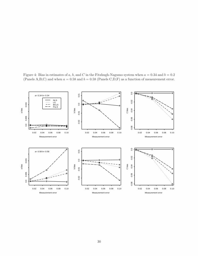
Figure 4: Bias in estimates of a, b, and C in the Fitzhugh-Nagumo system when a = 0.34 and b = 0.2(Panels A,B,C) and when a = 0.58 and b = 0.58 (Panels C,D,F) as a function of measurement error.

Measurement error

a bi

as

0.02 0.04 0.06 0.08 0.10

0.0

0.00

50.

015

NLSLSBCLSPsLS

a= 0.34 b= 0.34

Measurement error

b bi

as

0.02 0.04 0.06 0.08 0.10

-0.0

2-0

.01

0.0

0.01

Measurement error

C b

ias

0.02 0.04 0.06 0.08 0.10-0

.08

-0.0

6-0

.04

-0.0

20.

0

Measurement error

a bi

as

0.02 0.04 0.06 0.08 0.10

0.0

0.00

50.

015

a= 0.58 b= 0.58

Measurement error

b bi

as

0.02 0.04 0.06 0.08 0.10

-0.0

2-0

.01

0.0

0.01

Measurement error

C b

ias

0.02 0.04 0.06 0.08 0.10

-0.0

8-0

.06

-0.0

4-0

.02

0.0

30

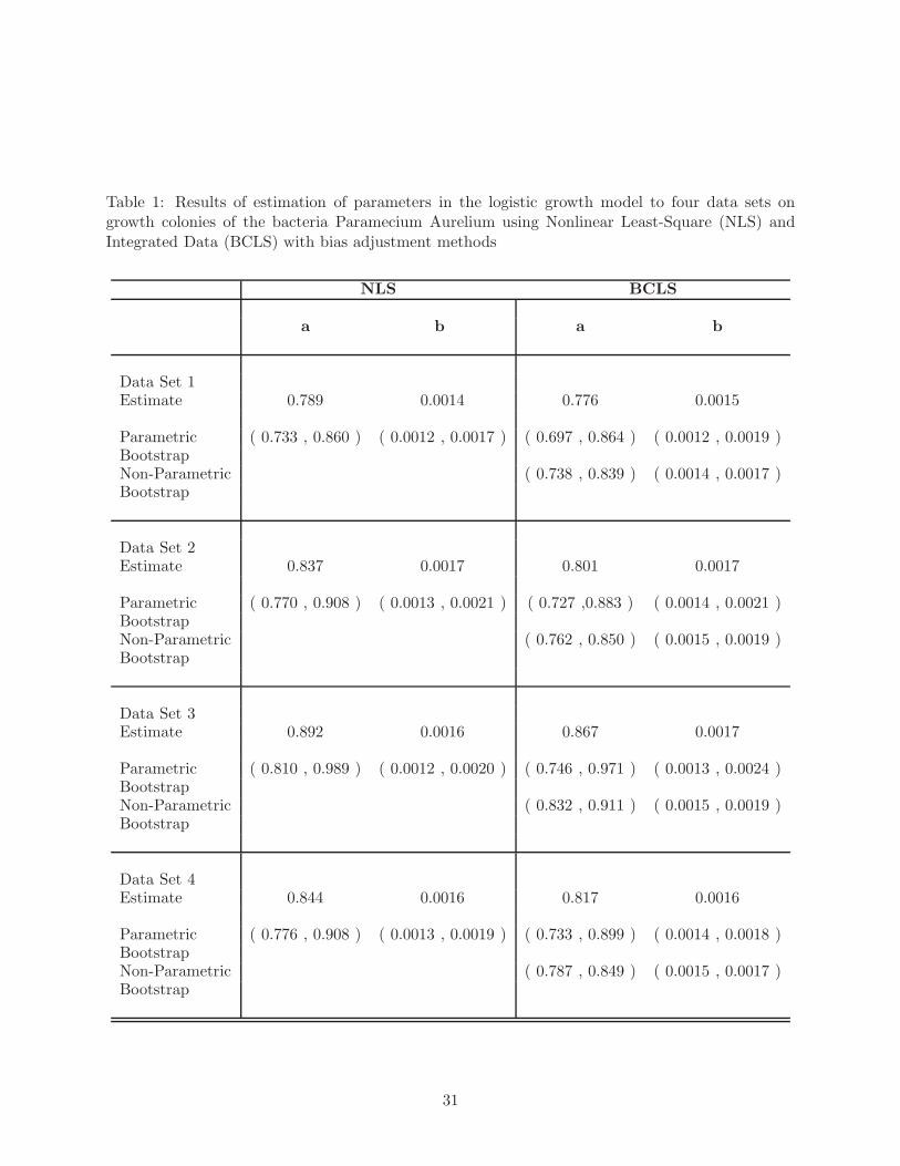
Table 1: Results of estimation of parameters in the logistic growth model to four data sets ongrowth colonies of the bacteria Paramecium Aurelium using Nonlinear Least-Square (NLS) andIntegrated Data (BCLS) with bias adjustment methods

NLS BCLS

a b a b

Data Set 1Estimate 0.789 0.0014 0.776 0.0015

Parametric ( 0.733 , 0.860 ) ( 0.0012 , 0.0017 ) ( 0.697 , 0.864 ) ( 0.0012 , 0.0019 )BootstrapNon-Parametric ( 0.738 , 0.839 ) ( 0.0014 , 0.0017 )Bootstrap

Data Set 2Estimate 0.837 0.0017 0.801 0.0017

Parametric ( 0.770 , 0.908 ) ( 0.0013 , 0.0021 ) ( 0.727 ,0.883 ) ( 0.0014 , 0.0021 )BootstrapNon-Parametric ( 0.762 , 0.850 ) ( 0.0015 , 0.0019 )Bootstrap

Data Set 3Estimate 0.892 0.0016 0.867 0.0017

Parametric ( 0.810 , 0.989 ) ( 0.0012 , 0.0020 ) ( 0.746 , 0.971 ) ( 0.0013 , 0.0024 )BootstrapNon-Parametric ( 0.832 , 0.911 ) ( 0.0015 , 0.0019 )Bootstrap

Data Set 4Estimate 0.844 0.0016 0.817 0.0016

Parametric ( 0.776 , 0.908 ) ( 0.0013 , 0.0019 ) ( 0.733 , 0.899 ) ( 0.0014 , 0.0018 )BootstrapNon-Parametric ( 0.787 , 0.849 ) ( 0.0015 , 0.0017 )Bootstrap

31

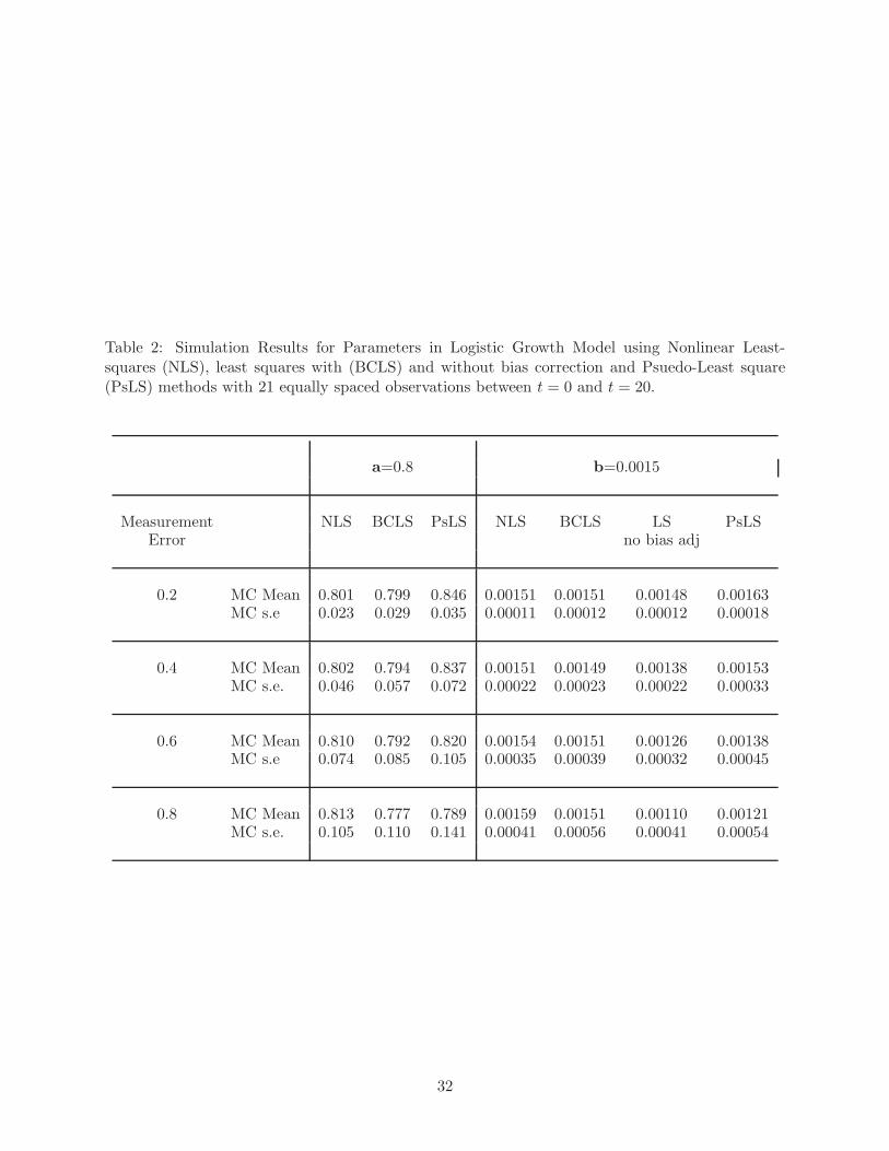
Table 2: Simulation Results for Parameters in Logistic Growth Model using Nonlinear Least-squares (NLS), least squares with (BCLS) and without bias correction and Psuedo-Least square(PsLS) methods with 21 equally spaced observations between t = 0 and t = 20.

a=0.8 b=0.0015

Measurement NLS BCLS PsLS NLS BCLS LS PsLSError no bias adj

0.2 MC Mean 0.801 0.799 0.846 0.00151 0.00151 0.00148 0.00163MC s.e 0.023 0.029 0.035 0.00011 0.00012 0.00012 0.00018

0.4 MC Mean 0.802 0.794 0.837 0.00151 0.00149 0.00138 0.00153MC s.e. 0.046 0.057 0.072 0.00022 0.00023 0.00022 0.00033

0.6 MC Mean 0.810 0.792 0.820 0.00154 0.00151 0.00126 0.00138MC s.e 0.074 0.085 0.105 0.00035 0.00039 0.00032 0.00045

0.8 MC Mean 0.813 0.777 0.789 0.00159 0.00151 0.00110 0.00121MC s.e. 0.105 0.110 0.141 0.00041 0.00056 0.00041 0.00054

32

Table 3: Simulation Results for Parameters in FitzHugh-Nagamu Model. Least squares withoutbias correction (LS). Bias-corrected least squares (BCLS). Psuedo least squares with smoothingbandwidth 0.2 (PsLS bw = 0.2). Psuedo least squares with smoothing bandwidth 0.37 (PsLS bw= 0.37).

Actual a = 0.34 b = 0.2 C = 3 v0 =-1 r0 =1

mean bias mean bias mean bias mean bias mean bias(s.e.) (s.e.) (s.e.) (s.e.) (s.e.)

LS 0.340 -0.001 0.200 0.002 2.958 -0.014 -0.936 -0.064 1.013 0.013( 0.004 ) ( 0.014 ) ( 0.086 ) ( 0.281 ) ( 0.030 )

BCLS 0.340 0.000 0.200 0.001 2.967 -0.011 -0.984 -0.016 1.010 0.010( 0.004 ) ( 0.013 ) ( 0.084 ) ( 0.280 ) ( 0.029 )

PsLS bw = 0.2 0.340 -0.001 0.199 -0.007 2.973 -0.009 NA NA( 0.024 ) ( 0.042 ) ( 0.045 )

PsLS bw = 0.37 0.336 -0.013 0.206 0.028 3.056 0.019 NA NA( 0.013 ) ( 0.029 ) ( 0.046 )

Actual a = 0.58 b = 0.58 C = 3 v0 =-1 r0 =1

LS 0.581 0.002 0.578 -0.003 2.938 -0.021 -0.892 -0.108 1.020 0.020( 0.005 ) ( 0.014 ) ( 0.118 ) ( 0.248 ) ( 0.041 )

BCLS 0.581 0.002 0.579 -0.002 2.948 -0.017 -0.966 -0.034 1.017 0.017( 0.005 ) ( 0.014 ) ( 0.122 ) ( 0.242 ) ( 0.042 )

PsLS bw = 0.2 0.585 0.008 0.577 -0.005 2.959 -0.014 NA NA( 0.025 ) ( 0.057) ( 0.060 )

PsLS bw = 0.37 0.581 0.002 0.573 -0.012 3.025 0.008 NA NA( 0.016 ) ( 0.036) ( 0.065 )

33

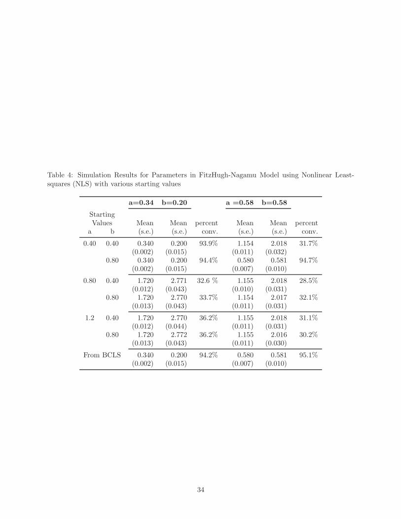
Table 4: Simulation Results for Parameters in FitzHugh-Nagamu Model using Nonlinear Least-squares (NLS) with various starting values

a=0.34 b=0.20 a =0.58 b=0.58

StartingValues Mean Mean percent Mean Mean percent

a b (s.e.) (s.e.) conv. (s.e.) (s.e.) conv.

0.40 0.40 0.340 0.200 93.9% 1.154 2.018 31.7%(0.002) (0.015) (0.011) (0.032)

0.80 0.340 0.200 94.4% 0.580 0.581 94.7%(0.002) (0.015) (0.007) (0.010)

0.80 0.40 1.720 2.771 32.6 % 1.155 2.018 28.5%(0.012) (0.043) (0.010) (0.031)

0.80 1.720 2.770 33.7% 1.154 2.017 32.1%(0.013) (0.043) (0.011) (0.031)

1.2 0.40 1.720 2.770 36.2% 1.155 2.018 31.1%(0.012) (0.044) (0.011) (0.031)

0.80 1.720 2.772 36.2% 1.155 2.016 30.2%(0.013) (0.043) (0.011) (0.030)

From BCLS 0.340 0.200 94.2% 0.580 0.581 95.1%(0.002) (0.015) (0.007) (0.010)

34