a fischer-tropsch synthesis reactor model framework for ... · a fischer-tropsch synthesis reactor...

SANDIA REPORTSAND2012-7848Unlimited ReleasePrinted September 2012

A Fischer-Tropsch Synthesis Reactor Model Framework for Liquid Biofuels ProductionJoseph W. Pratt

Prepared bySandia National LaboratoriesAlbuquerque, New Mexico 87185 and Livermore, California 94550

Sandia National Laboratories is a multi -program laboratory managed and operated by Sandia Corporation, a wholly owned subsidiary of Lockheed Martin Corporation, for the U.S. Department of Energy's National Nuclear Security Administration under contract DE-AC04-94AL85000.

Approved for public release; further dissemination unlimited.

2

Issued by Sandia National Laboratories, operated for the United States Department of Energy by Sandia Corporation.

NOTICE: This report was prepared as an account of work sponsored by an agency of the United States Government. Neither the United States Government, nor any agency thereof, nor any of their employees, nor any of their contractors, subcontractors, or their emplo yees, make any warranty, express or implied, or assume any legal liability or responsibility for the accuracy, completeness, or usefulness of any information, apparatus, product, or process disclosed, or represent that its use would not infringe privately owned rights. Reference herein to any specific commercial product, process, or service by trade name, trademark, manufacturer, or otherwise, does not necessarily constitute or imply its endorsement, recommendation, or favoring by the United States Government, any agency thereof, or any of their contractors or subcontractors. The views and opinions expressed herein do not necessarily state or reflect those of the United States Government, any agency thereof, or any of their contractors.

Printed in the United States of America. This report has been reproduced directly from the best available copy.

Available to DOE and DOE contractors fromU.S. Department of EnergyOffice of Scientific and Technical InformationP.O. Box 62Oak Ridge, TN 37831

Telephone: (865) 576-8401Facsimile: (865) 576-5728E-Mail: [email protected] ordering: http://www.osti.gov/bridge

Available to the public fromU.S. Department of CommerceNational Technical Information Service5285 Port Royal Rd.Springfield, VA 22161

Telephone: (800) 553-6847Facsimile: (703) 605-6900E-Mail: [email protected] order: http://www.ntis.gov/help/ordermethods.asp?loc=7-4-0#online

mailto:[email protected]

http://www.osti.gov/bridge

mailto:[email protected]

http://www.ntis.gov/help/ordermethods.asp?loc=7-4-0#online

3

SAND2012-7848 Unlimited Release

Printed September 2012

A Fischer-Tropsch Synthesis Reactor Model Framework for Liquid Biofuels

Production

Joseph W. Pratt

Energy Systems Engineering & Analysis Department (8366) Sandia National Laboratories

P.O. Box 969 Livermore, California, 94551

Abstract Fischer-Tropsch synthesis (FTS) is an attractive option in the process of converting biomass-derived syngas to liquid fuels in a small-scale mobile bio-refinery. Computer simulation can be an efficient method of designing a compact FTS reactor, but no known comprehensive model exists that is able to predict performance of the needed non-traditional designs.

This work developed a generalized model framework that can be used to examine a variety of FTS reactor configurations. It is based on the four fundamental physics areas that underlie FTS reactors: momentum transport, mass transport, energy transport, and chemical kinetics, rather than empirical data of traditional reactors.

The mathematics developed were applied to an example application and solved numerically using COMSOL. The results compare well to the literature and give insights into the operation of FTS that are then used to propose a new reactor concept that may be suitable for the mobile bio-refinery application.

4

Acknowledgements I am deeply grateful to the Sandia LDRD office and the ECIS investment area for sponsoring this project.

I would also like to thank the following people who participated in this project:

• Chris Shaddix for his mentorship, both technically and personally, throughout the project. • Hank Westrich and Sheri Martinez at the LDRD Office for their assistance and encouragement. • Daniel Dedrick for his work in forming the concept of this LDRD topic. • Blake Simmons for providing project management so I could focus on the technical challenges. • Deanna Agosta for financial planning. • Tiffany Vargas and Karen McWilliams at the CA Technical Library for providing and/or helping

me find the countless papers and texts used to develop my understanding of everything from the detailed theory to the history and applications of FTS.

5

Summary Liquid fuels synthesized from renewable CO and H2 could displace petroleum-based fuels to provide clean, renewable energy for the future. Small scale (<20 bbl/day) reactors for synthetic liquid fuels production are an emerging development area that may enable mobile biomass-to-liquids plants suited for on-demand liquid fuel production from diverse, underutilized, local resources. The design of such a “mobile bio-refinery” is a significant departure from the traditional large-scale industrial designs and requires predictive tools such as computer models to efficiently produce a successful facility. Because existing models inherently incorporate the empirical results of the traditional designs they are not suitable for this application. The need for a model that can examine the drastic design changes and innovations needed for the mobile bio-refinery is clear.

The goal of this work was to create a gas-to-liquids synthesis model with the minimum amount of empiricism and assumptions allowed by the current state of the theory, through integrated physics component models across varying length scales, with the ultimate purpose being to enable design of efficient, durable, and flexible small scale and/or novel reactors. Accomplishing this requires multiscale heat and mass transport models accounting for inter- and intra-particle gradients, coupled with generalized chemical kinetics models and dynamic (time-variant) degradation phenomena. There is no evidence in the open literature of a model of this type being successfully developed.

There are many pathways to producing liquid fuels such as gasoline, diesel, jet fuel, and their equivalents from biomass. A process incorporating Fischer-Tropsch Synthesis (FTS) may be more favorable than corn-based biofuels and cellulosic ethanol production. Accordingly, this work focuses on FTS as the technology of choice for gas-to-liquids synthesis.

“Fischer-Tropsch Synthesis” is the name given to an aggregate of simultaneous chemical reactions that produce hydrocarbons from the molecules CO and H2. Despite over 80 years of research in this field, the exact chemical mechanisms for these reactions are unknown and theories are still debated in the literature. As part of the work described in this report, a thorough examination of the literature was undertaken in the areas of reactor design, experiments or demonstrations of FTS, and modeling of the FTS process.

Consolidating the knowledge of many workers in the literature into a comprehensive mathematical model and then implementing that model into a numerical solving routine was the focus of this project. The particular fundamental physics areas examined are momentum transport (convection), mass transport (diffusion), energy transport (heat transfer), and chemical reaction kinetics. When developing the mathematical model, an example application and corresponding physical geometry was used to help in the process. In this case, the example application was a representative tube from a multi-tubular fixed bed reactor. Although this geometry was the only one explored in this work, the equations and physics can be generally applied to other geometries (as long as the underlying assumptions are not violated) and that is the ultimate intent of this model

The developed mathematical model was solved numerically using the software COMSOL. COMSOL has the ability to solve a wide variety of physics including all of those encountered in this framework. The

6

complex interaction of the physics during solving is something that is handled automatically by COMSOL when the numerical model is set correctly. COMSOL also includes extensive meshing ability and a wide variety of built-in solving routines that can handle the complex problems it sees, which can also be modified and optimized by the user if needed.

The model framework was applied to a 2-D axisymmetric representation of a single tube of a fixed bed reactor. There are examples in the literature of others simulating the heat and mass transfer of a similar problem, and the results of the model developed here compared very well to those. In addition to the results used for comparison, this model is also able to predict steady-state results for species concentrations, reaction rates, density, and liquid content. These are presented for further insight into the operation of the fixed bed reactor under the simulated conditions. The lessons learned from this simulation of the traditional fixed bed reactor tube were then used to propose a new design for a compact reactor suitable for a mobile bio-refinery.

Although the mathematical model as implemented in the COMSOL software was able to predict FTS behavior in the example application, there is still an opportunity to improve it in two general areas: (1) increased accuracy, and (2) faster and more robust solving capability. Incremental improvements to the model framework can be made through work in any of these areas.

7

Contents Abstract ......................................................................................................................................................... 3

Acknowledgements ....................................................................................................................................... 4

Summary ....................................................................................................................................................... 5

Figures ......................................................................................................................................................... 10

Tables .......................................................................................................................................................... 14

Nomenclature ............................................................................................................................................. 15

1 Introduction ........................................................................................................................................ 17

1.1 Description of the Problem ......................................................................................................... 17

1.2 Goal and Approach of the Study ................................................................................................. 18

1.3 Organization of the Report ......................................................................................................... 19

2 Introduction to Fischer-Tropsch Technology ...................................................................................... 21

2.1 The FTS Reaction ......................................................................................................................... 21

2.2 Influencing the FTS Reaction: Selectivity .................................................................................... 23

2.3 FTS Catalysts and Reactors ......................................................................................................... 27

2.4 Processing the FTS Product ......................................................................................................... 29

2.5 Current Facilities ......................................................................................................................... 31

3 Fischer-Tropsch Research ................................................................................................................... 41

3.1 Origins ......................................................................................................................................... 41

3.2 Current ........................................................................................................................................ 42

3.2.1 Reactor Design .................................................................................................................... 42

3.2.2 Experiments ........................................................................................................................ 46

3.2.3 Modeling ............................................................................................................................. 48

4 Mathematical Model .......................................................................................................................... 59

4.1 Governing Equations ................................................................................................................... 60

4.1.1 Mass Transport (Diffusion) ................................................................................................. 60

4.1.2 Momentum Transport (Convection) ................................................................................... 61

4.1.3 Energy Transport (Heat Transfer) ....................................................................................... 62

4.2 Boundary Conditions ................................................................................................................... 63




8

4.3 Initial Conditions ......................................................................................................................... 65




4.4 Chemical Reaction and Kinetics .................................................................................................. 65

4.4.1 The Fischer-Tropsch Synthesis Reactions ........................................................................... 65

4.4.2 The Water Gas Shift Reaction ............................................................................................. 67

4.4.3 The Phase Change Reactions .............................................................................................. 67

4.5 Constitutive Relations ................................................................................................................. 69

4.5.1 Density ................................................................................................................................ 69

4.5.2 Enthalpy .............................................................................................................................. 69

4.5.3 Diffusivity ............................................................................................................................ 70

4.5.4 Viscosity .............................................................................................................................. 71

4.5.5 Specific Heat ........................................................................................................................ 71

4.5.6 Thermal Conductivity .......................................................................................................... 72

5 Numerical Model ................................................................................................................................ 73

5.1 Modeling Platform ...................................................................................................................... 73

5.2 Built-in Physics ............................................................................................................................ 73

5.2.1 Darcy’s Law ......................................................................................................................... 73

5.2.2 Coefficient Form PDE .......................................................................................................... 73

5.2.3 Transport of Diluted Species ............................................................................................... 74

5.2.4 Transport of Concentrated Species..................................................................................... 74

5.2.5 Heat Transfer ...................................................................................................................... 74

5.3 User-Defined Functions and Variables ........................................................................................ 74

5.4 Implementing Multi-Physics Integration .................................................................................... 75

5.5 Solution Methods ........................................................................................................................ 75

6 Simulation Results of Example Application......................................................................................... 77

6.1 Physical Setup ............................................................................................................................. 77

6.2 Results ......................................................................................................................................... 78

6.3 Discussion .................................................................................................................................... 90

7 Conclusions and Future Work ............................................................................................................. 93

7.1 Conclusions ................................................................................................................................. 93

9

7.2 Future Work ................................................................................................................................ 94

References .................................................................................................................................................. 97

Appendix A: User Defined Functions ........................................................................................................ 102

Appendix B: Selected Variables ................................................................................................................ 106

Distribution ............................................................................................................................................... 108

10

Figures Figure 1: Dow Chemical Co.’s analysis of DOE data showing the total production costs of options

to generate liquid transportation fuels. Fischer-Tropsch synthesis is included in the gas-to-liquids (GTL) and coal-to-liquids (CTL) categories. Figure from [3], reprinted by [4]. ......................... 21

Figure 2: Anderson-Schulz-Flory (ASF) distribution for α = 0.9, showing the weight percent of each carbon-number species in the FT product. .................................................................................. 23

Figure 3: Anderson-Schulz-Flory (ASF) distribution in terms of mole percent, for α = 0.9. ....................... 24

Figure 4: Theoretical ASF distributions for three different FT reactors: High-temperature FT (HTFT), and two low-temperature FT (LTFT) processes. Note that the HTFT and LTFT vertical scales are different. In spite of the imperfections of the theory, it still clearly shows qualitative differences in the product from the three processes. Figure from de Klerk and Furimsky [7]. ......................................................................................................................................... 25

Figure 5: The four types of FT reactors used in most industrial facilities. Figure from de Klerk and Furimsky [7]. ......................................................................................................................................... 28

Figure 6: Schematic of a refinery for processing HTFT syncrude. Figure from de Klerk and Furimsky [7]. They note that these are typical refining pathways and this diagram does not represent any specific refinery. ............................................................................................................ 30

Figure 7: Sasol 1, in Sasolburg, So. Africa. Original design of 6,750 bbl/day crude oil equivalent. Currently using Fe-LTFT SBC and Fe-LTFT fixed bed reactors with natural gas feed. .......................... 35

Figure 8: Sasol 2 & 3, in Secunda So. Africa. 120,000 bbl/day crude oil equivalent from coal, currently via Fe-HTFT FFB units, primary product is gasoline. ............................................................. 35

Figure 9: Mossgas GTL in Mossel Bay, So. Africa. 24,000 bbl/day crude oil equivalent, primary products of gasoline and diesel, natural gas feed, using Fe-HTFT CFB reactors. ................................. 36

Figure 10: Shell Pearl in Ras Laffan, Qatar. 140,000 bbl/day crude oil equivalent from the two Co-LTFT fixed bed units. Primary product is distillate. ........................................................................ 36

Figure 11: Oryx GTL in Ras Laffan, Qatar. Designed for 34,000 bbl/day crude oil equivalent from natural gas, using Co-LTFT SBC reactors. Primary product is distillate. .............................................. 37

Figure 12: Syntroleum Catoosa demonstration plant. 70 bbl/day crude oil equivalent with two SBC reactors and natural gas feed. The plant was decommissioned in 2006. The primary product was diesel for blending. .......................................................................................................... 37

Figure 13: Rentech’s Product Demonstration Unit in Commerce City, CO. It uses the “Rentech reactor,” a Fe-LTFT SBC technology to produce 7-10 bbl/day crude oil equivalent. The unit is a test bed so feedstock is currently natural gas or petroleum coke and the products are primarily jet fuel and diesel. ................................................................................................................. 38

Figure 14: Velocys microtubular reactor. ................................................................................................... 38

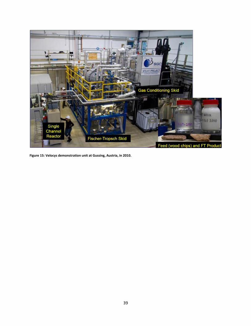
Figure 15: Velocys demonstration unit at Gussing, Austria, in 2010. ......................................................... 39

11

Figure 16: Number of archival publications containing the phrase “Fischer Tropsch” since 1925. ........... 41

Figure 17: Schematic of a multi-tubular fixed bed reactor, used as the example application for model development. ............................................................................................................................ 59

Figure 18: A 2-D axisymmetric plane of a representative tube is the geometric basis of the mathematical model. ........................................................................................................................... 60

Figure 19: Coarse mesh (750 elements) used during initial stages of solving. Note that the r-axis is stretched; both r and z axes are units of meters. The axis of symmetry is shown by the red dashed line at r=0. ................................................................................................................................ 76

Figure 20: Finer mesh (2,250 elements) used for solving the complete model. The added resolution in the r-direction is to capture the thermal transient that propagates inward from the exterior wall at r = 0.023 m. ........................................................................................................... 76

Figure 21: 2-D axisymmetric view of the pressure and temperature inside the tube at steady-state. A hot spot in the reactor can be seen at approximately r = 0 and z = 9.5 m, or at the center about 2.5 m from the inlet. ....................................................................................................... 78

Figure 22: 3-D view of the pressure and temperature inside the tube at steady-state. The region of the hot spot in the reactor is zoomed in on the left. ....................................................................... 79

Figure 23: From the results shown, for Tin,cool = 240 °C, it is expected that the hot spot will occur approximately 2 m from the inlet and reach a temperature between 280 °C and 320 °C. Figure 5 from Jess and Kern [42]. ......................................................................................................... 80

Figure 24: From the results shown, the maximum temperature at the centerline for Tin,cool = 240 °C is approximately 290 ° C. Figure 8 from Jess and Kern [42]. ........................................................... 80

Figure 25: The liquid fraction. The liquid is close to the wall in an annular ring, with the center filled with gas. As pressure decreases down the tube, some liquid changes to gas. Although the temperature profile is relatively constant in the radial direction after the hot-spot at z = 9.5 m, the liquid stays near the outer wall because there is no radial movement of the bulk fluid. The distribution of the primary liquid species C7H16 and C8H18 are shown in Figure 38 and Figure 41, respectively................................................................................................................... 81

Figure 26: The density. Density follows liquid fraction (Figure 25) closely, but is more influenced by the decrease in pressure from reactor inlet to outlet. .................................................................... 82

Figure 27: Rate of the water-gas shift reaction (Eq. (46)). For z < 9.5, the reaction rate is slightly negative in the entire reactor due to the absence of CO, which was consumed at z = 9.5. As soon as more CO is produced, it is consumed by the FT reaction, so the WGS reaction rate remains negative while z < 9.5. When z > 9.5 m, the reaction rate varies in the radial direction, increasing in the direction of decreasing temperature. This correct yet counterintuitive result arises because the WGS reaction indeed behaves this way at conditions encountered: very low water concentrations (cH2O ≅ 0.01) combined with high H2 and CO concentrations. ................................................................................................................... 82

12

Figure 28: The Fischer-Tropsch reaction rate (Eq. (43)). The bulk of the FT reaction occurs at 2.5 m from the inlet. After that, although there is H2 present, all the CO is consumed (see Figure 30), only being produced by a slight WGS reaction, so the FT reaction rate is positive but very slow. The independence of FT reaction rate on temperature is not realistic, but does correspond to the parameter used for kFT in Eq. (43). As mentioned there, a better expression incorporating a temperature dependence could be easily implemented once known. .................................................................................................................................................. 83

Figure 29: Hydrogen concentration tracks its production via the WGS reaction and its consumption via the FT reaction. The trend of gradual decrease from z = 9.5 towards the exit is mostly due to the decreasing pressure, which causes a lower density and higher velocity, reducing the amount of gas present per unit volume ........................................................... 83

Figure 30: CO concentration. The effect of the WGS reaction on CO is small (notice no radial variation), so its concentration closely follows that of the FT reaction. By the time the reactants get to z = 9.5 m, all the CO is consumed. Since the WGS reaction is slightly negative for all z < 9.5, CO is being produced in this region but is immediately consumed by the FT reaction, and its concentration remains relatively constant. ................................................... 84

Figure 31: CO2 concentration. CO2 is produced via the FT reaction. The slight curvature near the wall is due to the WGS reaction. For z < 9.5, the slightly negative WGS reaction is slowly consuming CO2 which is evident in the gradually decreasing concentration towards the exit. .......... 84

Figure 32: Water (gas) concentration. The majority of H2O (g) is produced by the FT reaction. However, prior to z = 9.5, the water is consumed by the WGS reaction. The trend of gradual decrease from z = 9.5 towards the exit is mostly due to the decreasing pressure, which causes a lower density and higher velocity, reducing the amount of gas present per unit volume. ................................................................................................................................................. 85

Figure 33: Water (liquid) concentration. Liquid water is only present due to the equilibrium condition between phases which states that the phase which should be present due to the local temperature and pressure is 100-times the phase which should not be present at that condition. Thus, the liquid water content follows that of the gas almost identically. ........................ 85

Figure 34: CH4 concentration tracks the FT reaction rate. The trend of gradual decrease from z = 9.5 towards the exit is mostly due to the decreasing pressure, which causes a lower density and higher velocity, reducing the amount of gas present per unit volume. ........................................ 86

Figure 35: C6H14 (gas) concentration follows that of the FT reaction rate and the trend is nearly identical to that of CH4, although the amount (moles) of C6H14 produced is much smaller, as expected. .............................................................................................................................................. 86

Figure 36: C6H14 (liquid) concentration. Liquid C6H14 is only present due to the equilibrium condition between phases which states that the phase which should be present due to the local temperature and pressure is 100-times the phase which should not be present at that condition. Thus, the C6H14 liquid content trend follows that of the gas almost identically. ............... 87

13

Figure 37: C7H16 (gas) concentration. For the most part, C7H16 gas phase is minor, although there is some present when the temperature reaches its peak at z = 9.5 m. ............................................... 87

Figure 38: C7H16 (liquid) concentration. C7H16 is present mainly in the liquid phase. The high concentration of C7H16 near the wall is likely due to an overall flux of C7H16 away from the center for z > 9.5, as shown in Figure 39. ............................................................................................. 88

Figure 39: Overall radial flux (diffusive and convective) of C7H16, both gas and liquid phase. Zero flux is colored white, positive is a red shade, and negative (toward the center) is a blue shade. It can be seen that there is an overall flux of C7H16 from the center to the edge when z > 9.5. This is the most likely explanation for the build-up of C7H16 near the wall as shown in Figure 38. .............................................................................................................................................. 88

Figure 40: C8H18 (gas) concentration. Only a small amount of C8H18 gas is present, at the hot spot at z = 9.5 m. Even then, the concentration is very small compared to the liquid concentration as seen in Figure 41. ..................................................................................................... 89

Figure 41: C8H18 (liquid) concentration. Similar to the C7H16 case, there is more C8H18 present near the wall than the centerline. Figure 42 shows that there is an overall radial flux of C8H18 which is the likely explanation for this result. ...................................................................................... 89

Figure 42: Overall radial flux (diffusive and convective) of C8H18, both gas and liquid phase. Zero flux is colored white, positive is a red shade, and negative (toward the center) is a blue shade. It can be seen that there is an overall flux of C8H18 from the center to the edge when z > 9.5, although the effect is not as pronounced as the C7H16 case. This is the most likely explanation for the radial variation in concentration as shown in Figure 41. ..................................... 90

Figure 43: Potential FT reactor concept suitable for a mobile bio-refinery. .............................................. 91

14

Tables Table 1: Relationship between common product categories and carbon number of primary

constituents. ......................................................................................................................................... 25

Table 2: Efect of operating parameters on FTS process selectivity. ........................................................... 26

Table 3: Generalized property comparison of FT syncrudes and conventional crude oil. Table from de Klerk and Furimsky [7]. ........................................................................................................... 30

Table 4: Commonly used crude oil refining technologies and catalysts, and their compatibility with FT syncrude. Neutral and Good indicate possible efficient use in FT syncrude refining, while Poor indicates some inefficiency. Table from de Klerk and Furimsky [7]. ................................. 31

Table 5: Summary of commercial FT facilities ............................................................................................ 33

Table 6: Summary of hydrogen reaction orders (experiment based) ........................................................ 49

Table 7: Summary of relevant kinetic models ............................................................................................ 52

Table 8: Physical parameters of the example application. Unless noted otherwise, values are taken from Jess and Kern [42]. ............................................................................................................. 77

15

Nomenclature Default units are given in brackets [] when applicable. In some cases, other definitions or units are used for the same variable. These are denoted in the text where it occurs.

Acronyms ASF Anderson-Schulz-Flory BTL Biomass-to-liquids CFB Circulating fluidized bed CSTR Continually stirred tank reactor CTL Coal-to-liquids CW Cooling water FFB Fixed fluidized bed FT Fischer-Tropsch FTS Fischer-Tropsch Synthesis GTL (Natural) Gas-to-liquids HTFT High temperature Fischer-Tropsch LHHW Langmuir-Hinshelwood-Hougen-Watson LTFT Low temperature Fischer-Tropsch PDE Partial differential equation SBC Slurry bubble column SBR Spinning basket reactor WGS Water-gas shift Symbols Cp Specific heat at constant pressure [J/(kg*K)] ci Concentration of species i [mol/m3] cx Fluid content of fluid x [kg/m3] Di Diffusion coefficient of species I [m2/s] f Source term in general PDE hi Enthalpy of species i [J/mol] ji Flux of species i [mol/(m2*s) or kg/m2*s) depending on context] Keq Equilibrium reaction rate [mol/(m3*s)] Kri Relative permeability of fluid i [-] k Thermal conductivity [W/(m*K)] ki Kinetic term in reaction rate. Units vary, see text. kf Forward reaction rate [mol/(m3*s)] kr Reverse reaction rate [mol/(m3*s)] Mi Molecular weight of species i [kg/mol] Mn Molecular weight of the mixture [kg/mol] P Pressure [Pa] Pc Critical pressure [Pa] pi Partial pressure of species i [Pa]

16

Q Heat source [W/m3] Qm Bulk production of fluid [kg/m3*s] R Gas constant [J/(K*mol)] Ri Production of species i [mol/(m3*s) or kg/m3*s) depending on context] r Radius [m] rA Rate of reaction A si Saturation of fluid i [-] T Temperature [K] Tc Critical temperature [K] t Time [s] u Velocity [m/s] Xi Selectivity of species i z Height [m] z Compressibility factor [-] Greek Letters α Chain growth probability [-] εp Bed porosity [-] φ Thiele modulus [-] φij Interaction coefficient between species i and j. φp Solid material’s volume fraction [-] κ Permeability of the porous medium [m2] µ Viscosity [Pa*s] ωi Mass fraction of species i [-] ρ Density [kg/m3]

17

1 Introduction Liquid fuels synthesized from renewable CO and H2 could displace petroleum-based fuels to provide clean, renewable energy for the future. Small scale (<20 bbl/day) reactors for synthetic liquid fuels production are an emerging development area that may enable mobile biomass-to-liquids plants suited for on-demand liquid fuel production from diverse, underutilized, local resources.

These “mobile bio-refineries” have applications both in the civilian and military sector. In civilian life, a truck-mounted facility could travel to locations, such as farms or forests, where waste biomass is available but is either too remote or is in quantities that are too small to make it cost-effective to be transported to a central processing facility. The mobile unit can convert the biomass to liquid fuel locally, either then transporting the energy-dense fuel or syncrude back to a central facility, or leaving the fuel on-site for direct local use.

In the military, the interest is primarily in the local production of usable fuel, in order to reduce the logistical burden of supplying fuel to combat bases and troops. The importance of this can be summarized by U.S. Army General David Petraeus in a memorandum sent in July, 2011 [1]:

“Our need for fuel … is greater than at any time in history. This ‘operational energy’ is the lifeblood of our warfighting capabilities. … Nearly 80% of ground supply movements are composed of fuel, and we have lost many lives delivering fuel to bases around Afghanistan. Moreover, moving and protecting this energy diverts forces away from combat operations.”

A primary method to produce liquid fuels from a CO + H2 syngas is Fischer-Tropsch synthesis (FTS), a concept that has existed for over 100 years and has been formalized to what is now known as FTS about 80 years ago (See Section 3.1 for more historical background). Finding the best conditions for production of liquid fuels in FTS is a continual fight between competing forces. In general, operating conditions (e.g., temperature, pressure, concentration, velocity), the factors that control them, and the physical parameters such as catalyst properties and reactor structure all have conflicting impacts on the goal of high production of liquid fuels.

1.1 Description of the Problem Over the last 80 years, the determination of optimal FTS reactor conditions has evolved starting with primarily experimentally-determined inputs, to more use of empirical modeling, to incorporation of more theory so that optimal conditions can be predicted and laboratory and pilot plant tests are no longer needed. However, although reactor size and capacity has increased over the years, the same general reactor design today is not much different than that used in the 1940’s, especially in the case of fixed-bed [2].

The FTS process involves very complicated physics of concurrent homogeneous and heterogeneous reactions, phase changes, and multiscale heat and mass transfer. Because of this, reactor development and analysis has traditionally relied not only on empirical correlations for their design but also on the availability of a wide variety of post-FT refining options that are not practically implementable in a mobile bio-refinery concept. The mobile bio-refinery reactors need to be designed at suitable scales and

18

must produce a suitable range of carbon chain lengths from the FT reactor itself, motivating the development of truly predictive FT process modeling capabilities based on first-principles descriptions of the relevant physics and chemistry. Such a model must be general enough to explore non-traditional designs while also being powerful enough to address the known issues of (1) non-uniform temperature distributions, (2) wax buildup, (3) conversion and selectivity optimization, and (4) lifecycle degradation.

1.2 Goal and Approach of the Study The goal of this work is:

To create a gas-to-liquids synthesis model with the minimum amount of empiricism and assumptions allowed by the current state of the theory, through integrated physics component models across varying length scales.

And the purpose is:

To enable design of efficient, durable, and flexible small scale and/or novel reactors.

Accomplishing this requires multiscale heat and mass transport models accounting for inter- and intra-particle gradients, coupled with generalized chemical kinetics models and dynamic (time-variant) degradation phenomena. There is no evidence in the open literature of a model of this type being successfully developed.

The different types of phenomena occurring in FTS lend themselves to a component-based modeling approach. In this method, component sub-models of each phenomenon are made and then integrated to obtain the model of the entire reactor. This component-model approach is a distinguishing factor from other efforts. The components of the developed model are:

1. Two-phase flow in a catalyst bed 2. Interparticle heat transfer 3. Interparticle mass transfer 4. FTS synthesis chemical kinetics

Intraparticle effects were not taken into account in the present model for simplicity. The model also has the ability to add-in an examination of time-dependent catalyst deactivation.

The development of each component model involves five inter-related steps:

1. Theoretical understanding 2. Equation reduction and empirical parameter minimization 3. Programming 4. Testing/debugging 5. Validation

The final task is to build the overall model. The three steps are (1) combination of component models, (2) testing and debugging, and (3) validation.

19

1.3 Organization of the Report After this introduction, Chapter 2 presents an introduction to Fischer-Tropsch Technology which includes both basic technical aspects as well as a review of current FT trends and facilities. Chapter 3 describes the scientific research over the years, with a focus on the latest developments that are most relevant to this modeling work. The fundamental mathematics upon which the model is based are presented in Chapter 4, and Chapter 5 describes the implementation of these mathematics into the software modeling platform COMSOL. Results of the simulations are presented and discussed in Chapter 6, and Conclusions and Recommendations are given in Chapter 7.

21

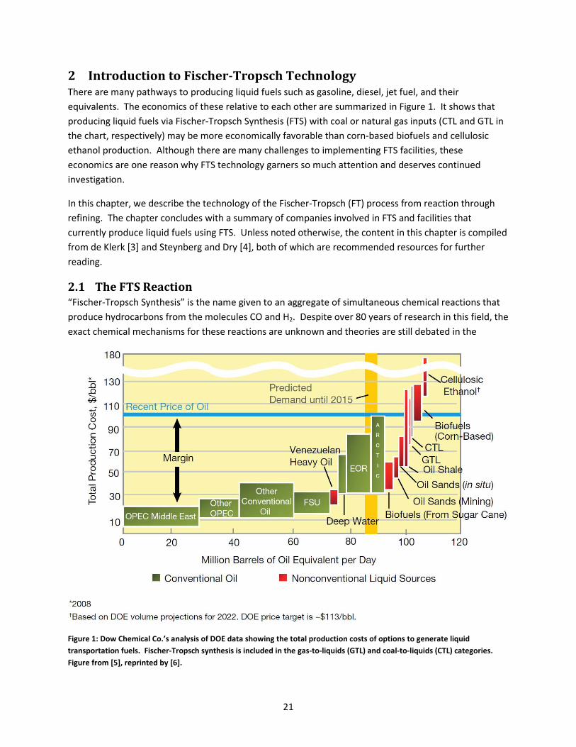
2 Introduction to Fischer-Tropsch Technology There are many pathways to producing liquid fuels such as gasoline, diesel, jet fuel, and their equivalents. The economics of these relative to each other are summarized in Figure 1. It shows that producing liquid fuels via Fischer-Tropsch Synthesis (FTS) with coal or natural gas inputs (CTL and GTL in the chart, respectively) may be more economically favorable than corn-based biofuels and cellulosic ethanol production. Although there are many challenges to implementing FTS facilities, these economics are one reason why FTS technology garners so much attention and deserves continued investigation.

In this chapter, we describe the technology of the Fischer-Tropsch (FT) process from reaction through refining. The chapter concludes with a summary of companies involved in FTS and facilities that currently produce liquid fuels using FTS. Unless noted otherwise, the content in this chapter is compiled from de Klerk [3] and Steynberg and Dry [4], both of which are recommended resources for further reading.

2.1 The FTS Reaction “Fischer-Tropsch Synthesis” is the name given to an aggregate of simultaneous chemical reactions that produce hydrocarbons from the molecules CO and H2. Despite over 80 years of research in this field, the exact chemical mechanisms for these reactions are unknown and theories are still debated in the

Figure 1: Dow Chemical Co.’s analysis of DOE data showing the total production costs of options to generate liquid transportation fuels. Fischer-Tropsch synthesis is included in the gas-to-liquids (GTL) and coal-to-liquids (CTL) categories. Figure from [5], reprinted by [6].

22

literature. However, it is generally agreed that CO and H2 react on a catalytic surface to produce a CH2 monomer according to the following net reaction:

CO + 2H2 -> -CH2- + H2O (1) If the CH2 monomer remains attached to the surface it polymerizes with another CH2 monomer and participates in “chain growth”. In polymerization, several CH2 monomers combine into chains that can theoretically be of any length. For example, three CH2 monomers can polymerize to form the molecule C3H6. The general formula to represent this overall result is:

nCO + 2nH2 -> (-CH2-)n + nH2O (2) where “n” is the number of monomers joined together in the chain, and is also the carbon number of the resulting species.

After every polymerization step the resulting polymer has the option to (1) continue in chain growth and remain on the surface, (2) terminate chain growth and detach from the surface as an olefin (alkene), or (3) terminate chain growth, hydrogenate (add another H2 molecule to the hydrocarbon) and detach from the surface as a paraffin (alkane). The termination steps are described by the termination-to-olefin reaction:

nCO + 2nH2 -> CnH2n + nH2O (3) and the termination-to-paraffin reaction:

nCO + (2n+1)H2 -> CnH2n+2 + nH2O (4) As can be expected in a catalytic reactor with many species present, there are also many other reactions that can take place. The most significant of these side reactions are the water-gas shift reaction:

CO + H2O <-> CO2 + H2 (5) and the formation of alcohols:

nCO + 2nH2 -> CnH2n+2O + (n-1)H2O (6) Other side reactions contribute to a very small portion of the product under normal operating conditions and are often ignored unless detailed mechanistic studies are the goal.

Overall, the net FTS reaction is highly exothermic and thermal runaway within a reactor can easily occur without a properly designed heat rejection method. Handling the large amount of heat generated by this process is a challenging design issue and, as will be discussed later, is a major reason for different reactor designs.

23

2.2 Influencing the FTS Reaction: Selectivity As illustrated by the FT reactions shown above, there are literally countless possible species that could result from FTS. Thus simply knowing the chemical reactions is not enough to predict the product of a given FT reactor. This opens the door to one of the most important concepts of FTS: the product selectivity.

Selectivity refers to the preference of the process to produce one molecule over another. On a carbon number basis it can be generally defined as:

(moles of hydrocarbon with carbon number n) * n / (total moles of CO and CO2 converted) (7)

This equation can be applied to single species, such as hexane (C6H14) or to groups (for example, all paraffins, or all products from C9 to C12 (jet fuel cut)).

The selectivity of a particular carbon number species has been theoretically described using the chain growth probability parameter α, which can vary from 0 (no chain growth) to 1 (infinite chain growth), through the Schulz-Flory equation:

xn = (1-α)*αn-1 (8) Calculating xn for every n from 1 upward gives the Anderson-Schulz-Flory (ASF) distribution. An example is shown here in Figure 2, where α has been set to 0.9. Note that the figure is given in terms of a mass

Figure 2: Anderson-Schulz-Flory (ASF) distribution for α = 0.9, showing the weight percent of each carbon-number species in the FT product.

0.0%

1.0%

2.0%

3.0%

4.0%

5.0%

0 5 10 15 20 25 30 35 40 45 50 55 60

Wei

ght P

erce

nt in

Pro

duct

Carbon Number

24

Figure 3: Anderson-Schulz-Flory (ASF) distribution in terms of mole percent, for α = 0.9.

basis, which literally ‘weights’ higher carbon number species more. Figure 3 shows the same data on a molar basis. It is evident that the most favored reactions are the light hydrocarbons, and this is true no matter what α value is used.

It must be noted that theoretical ASF distributions do not align with observation in several respects. First, the methane (CH4) selectivity is usually higher than predicted. Second, the C2 (ethene and ethane) selectivity is usually much lower than predicted. Finally, lower C-number products and higher C-number products seem to have their own, separate α values, which is most likely due to a difference between the probability of termination to olefin vs. termination to paraffin. Nevertheless, α-values are still commonly used to give a qualitative measure of the effectiveness of a particular reactor to produce the desired product, for example see Figure 4. Here it can be seen that lower α-values lead to an FTS product that is mostly light hydrocarbons, and higher α-values lead to FTS product that is medium-to-high weight hydrocarbons.

At this point it is easy to forget that the FTS product contains other species that are ignored when describing the carbon-number distribution. This includes un-reacted CO and H2, which may be as much as 50% of that in the inlet stream; water, which is produced at a volume approximately equal to that of the total hydrocarbon amount; and CO2 which is an unusable diluent. Considering all of these products, it is easy to see that the oft-discussed “FTS product” (i.e., the hydrocarbon part) is often less than 50% of the stream that actually comes out of the reactor.

0%

2%

4%

6%

8%

10%

12%

0 5 10 15 20 25 30 35 40 45 50 55 60

Mol

e Pe

rcen

t in

Prou

dct

Carbon Number

25

Figure 4: Theoretical ASF distributions for three different FT reactors: High-temperature FT (HTFT), and two low-temperature FT (LTFT) processes. Note that the HTFT and LTFT vertical scales are different. In spite of the imperfections of the theory, it still clearly shows qualitative differences in the product from the three processes. Figure from de Klerk and Furimsky [7].

The practical importance of selectivity comes from an understanding of the relationship of carbon numbers to saleable product. Table 1 shows the carbon number constituents of common hydrocarbon product categories. Note there is overlap as the products are not defined by their carbon number makeup, but rather by physical properties such as viscosity, boiling point, etc. One can imagine then that if a certain product is desired, say diesel fuel, that a FTS process with a selectivity towards carbon numbers 13-18 is probably preferred. However, a recent approach to production of middle-weight products is to operate the FTS process with a high a (> 0.9) such that mostly high-weight products like waxes are produced. These are then hydroprocessed in downstream equipment to achieve a more exact end-product carbon number distribution [8, 9].

Table 1: Relationship between common product categories and carbon number of primary constituents.

Product Category Carbon Number Range Tail gas C1 – C2

LPG C3 – C4 Gasoline/Naphtha C4 – C10

Jet Fuel C9 – C12 Distillate C11 – C22

Diesel C13 – C18 Light Wax C24 – C35

Heavy Wax C36+

26

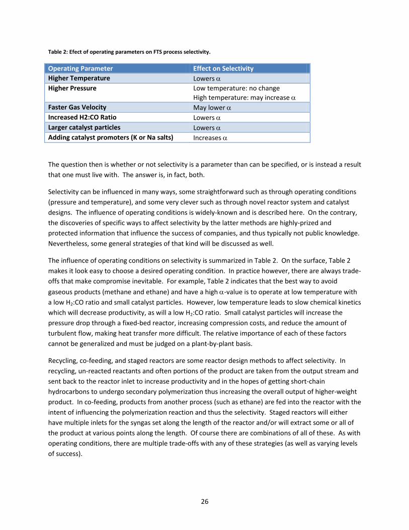
Table 2: Efect of operating parameters on FTS process selectivity.

Operating Parameter Effect on Selectivity Higher Temperature Lowers α Higher Pressure Low temperature: no change

High temperature: may increase α Faster Gas Velocity May lower α Increased H2:CO Ratio Lowers α Larger catalyst particles Lowers α Adding catalyst promoters (K or Na salts) Increases α

The question then is whether or not selectivity is a parameter than can be specified, or is instead a result that one must live with. The answer is, in fact, both.

Selectivity can be influenced in many ways, some straightforward such as through operating conditions (pressure and temperature), and some very clever such as through novel reactor system and catalyst designs. The influence of operating conditions is widely-known and is described here. On the contrary, the discoveries of specific ways to affect selectivity by the latter methods are highly-prized and protected information that influence the success of companies, and thus typically not public knowledge. Nevertheless, some general strategies of that kind will be discussed as well.

The influence of operating conditions on selectivity is summarized in Table 2. On the surface, Table 2 makes it look easy to choose a desired operating condition. In practice however, there are always trade-offs that make compromise inevitable. For example, Table 2 indicates that the best way to avoid gaseous products (methane and ethane) and have a high α-value is to operate at low temperature with a low H2:CO ratio and small catalyst particles. However, low temperature leads to slow chemical kinetics which will decrease productivity, as will a low H2:CO ratio. Small catalyst particles will increase the pressure drop through a fixed-bed reactor, increasing compression costs, and reduce the amount of turbulent flow, making heat transfer more difficult. The relative importance of each of these factors cannot be generalized and must be judged on a plant-by-plant basis.

Recycling, co-feeding, and staged reactors are some reactor design methods to affect selectivity. In recycling, un-reacted reactants and often portions of the product are taken from the output stream and sent back to the reactor inlet to increase productivity and in the hopes of getting short-chain hydrocarbons to undergo secondary polymerization thus increasing the overall output of higher-weight product. In co-feeding, products from another process (such as ethane) are fed into the reactor with the intent of influencing the polymerization reaction and thus the selectivity. Staged reactors will either have multiple inlets for the syngas set along the length of the reactor and/or will extract some or all of the product at various points along the length. Of course there are combinations of all of these. As with operating conditions, there are multiple trade-offs with any of these strategies (as well as varying levels of success).

27

Overall, while selectivity can be tailored in many ways, there are always limits to the amount of possible variation once certain operating conditions are chosen. For example, in a given reactor design with a specified catalyst, there are limits on how much the temperature can be changed without causing failure or gross inefficiency in another part of the process. Thus, selectivity should be thought of more as a parameter to be set in the initial stages of plant design and less of one that can be changed on a daily basis.

2.3 FTS Catalysts and Reactors At typical FTS conditions (pressure, temperature, and reactants), thermodynamic analysis of the reaction reveals that the primary products would CH4 and C. This fact illustrates not only that producing a liquid fuel from CO and H2 via FTS is a continual struggle against nature, but also the critical role the catalyst plays in avoiding the equilibrium condition.

The two catalysts used in practice for FTS are iron and cobalt. Cobalt generally costs more although the actual ratio between iron and cobalt varies. For example, the same author states Cobalt metal is about 230 times the cost of iron metal (in 1990, [10]), but this figure changes to 1,000-times the cost of iron metal in 2004 [11]. Either way, cobalt’s higher cost is often justified in two ways: (1) typically less is used because it has a higher activity than iron, and (2) it usually has longer lifetimes and higher productivity.

It is common to add other elements along with the base catalyst metal. This can include alkali promoters such as potassium and sodium salts, support materials for structural stability and increased surface area, and stabilizers such as silica. While the goals of any of these additives are straightforward, namely to increase lifetime, increase productivity, and tailor the selectivity, the optimal additive combinations are the subject of much research.

FTS reactors can be classified by their operating temperature and catalyst. The so-called low temperature (LTFT) reactors operate between 200°C and 250°C. The catalyst can be iron or cobalt, referred to as Fe-LTFT and Co-LTFT respectively. Relatively, Fe-LTFT reactors produce heavier products with medium olefin content and are used where distillates and waxes are desired. Co-LTFT reactors produce medium-weight products with low olefin content and are used where primarily distillates are desired.

The high temperature (HTFT) reactors operate between 320°C to 350°C and use iron as the catalyst. They produce lighter weight products with higher olefin content and are used where gasolines are desired.

The four types of reactors used in nearly all current FT facilities are shown in Figure 5. Fixed bed and slurry bubble column (SBC) reactors are LTFT-type with product in both liquid and gas phase. The fluidized bed reactors are HTFT-type with only gaseous product. Right away one can see that the choice of reactor will directly influence the achievable product distribution, as the fluidized bed reactors are restricted from producing any product that would condense below 350 °C (which corresponds to about C20 and above, see also the “HTFT” line in Figure 4).

28

Figure 5: The four types of FT reactors used in most industrial facilities. Figure from de Klerk and Furimsky [7].

Fixed bed reactors are basically shell-and-tube heat exchangers with the FTS occurring within the tubes and cooling water circulating through the shell to remove the heat. Typical dimensions may be 5 cm diameter tubes with 2-3 mm diameter catalyst particles, and the tube length could range from 2 m for lab-scale units to more than 10 m for large commercial units. Fixed bed reactors have the most challenging heat transfer issues which in practice are what limit the upper diameter of the tubes. It has also been found that high gas velocities lead to turbulent flow, which greatly enhances heat transfer through the fluid. This results in lower productivity and conversion but is the tradeoff for the simplicity of this reactor design.

A sub-set of fixed bed reactors are the microchannel type. These employ much smaller diameter “tubes” (that may in fact be a wide variety of shapes other than circular) and catalyst particles of 100 µm or less. This type of reactor has better heat and mass transfer characteristics than the large scale type and is marketed as being modular and more compact.

SBC reactors are vessels containing a slurry (liquid + solid) mixture of catalyst suspended in their own FT liquid product. Syngas is fed from the bottom and bubbles up through the mixture. The heat of reaction is rejected via cooling tubes that pass through the slurry. Heat transfer is greatly increased by the constant movement of the slurry, which is the primary reason this type of reactor is used. Gaseous product and leftover reactants are extracted out of the top and processed and/or recycled. Slurry is also continually extracted to remove liquid product, but since the slurry contains catalyst particles, effective separation of the two phases is mandatory and not trivial, and is the primary disadvantage of this type of reactor. Also, some catalyst is lost during this process. However, a side benefit to this procedure is

29

that because the catalyst is removed from the reactor at this point, it can either be regenerated or replaced before being sent back into the reactor. This enables the SBC reactor to theoretically never require shutdown for catalyst replacement, contrary to the fixed bed type. The fact that some catalyst is continually lost and must be replaced seems to indicate that SBC reactors are better suited for (cheaper) iron catalysts than (more expensive) cobalt, but there are two large-scale plants (Oryx and Escravos, see the Facilities sections for more information) that use cobalt SBCs, most likely because of the desired product slate.

The fluidized bed reactors operate entirely in the gas phase, with catalyst particles suspended by the upward movement of the flow. For both types of fluidized beds, catalyst is extracted while operating, eliminating the need to shut down for catalyst replacement. However, the requirement to operate in gas-phase restricts the formation of FT liquid product at operating conditions, inherently limiting these reactors to lower-α selectivities, as illustrated in Figure 4. Fixed fluidized bed (FFB) reactors are generally more difficult to control and have tighter restrictions on gas flow rate and catalyst particle size, but have been shown to be more efficient than circulating fluidized bed. Circulating fluidized bed (CFB) reactors theoretically have a wider operating window but in practice are subject to problems that sometimes negate this advantage. The circulating fluidized bed type also subjects catalyst particles to higher mechanical stresses as they are convected around the loop at several meters per second. While one of the first fluidized bed reactors was fixed (Hydrocol in 1950’s), subsequent ones were circulating (Sasol 1950’s to 1990’s), presumably because they were assumed to be simpler to operate. However, Sasol developed a “new” technology fixed fluidized bed and now that is the prevalent type again.

2.4 Processing the FTS Product When product distribution curves such as Figure 4 are combined with information such as in Table 1, it is easy to mistakenly believe that an FT reactor can directly produce “jet fuel,” “diesel,” or other products. In fact what these figures and tables show is simply the carbon number distribution in the product, and it is important to realize that having the correct carbon number is only one piece of the puzzle that makes up a usable fuel. The product of an FT reactor is not a usable fuel, but rather something analogous to crude oil that goes by the name “syncrude”. And like crude oil, syncrude must be refined before use.

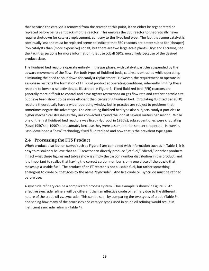
A syncrude refinery can be a complicated process system. One example is shown in Figure 6. An effective syncrude refinery will be different than an effective crude oil refinery due to the different nature of the crude oil vs. syncrude. This can be seen by comparing the two types of crude (Table 3), and seeing how many of the processes and catalyst types used in crude oil refining would result in inefficient syncrude refining (Table 4).

30

Figure 6: Schematic of a refinery for processing HTFT syncrude. Figure from de Klerk and Furimsky [7]. They note that these are typical refining pathways and this diagram does not represent any specific refinery.

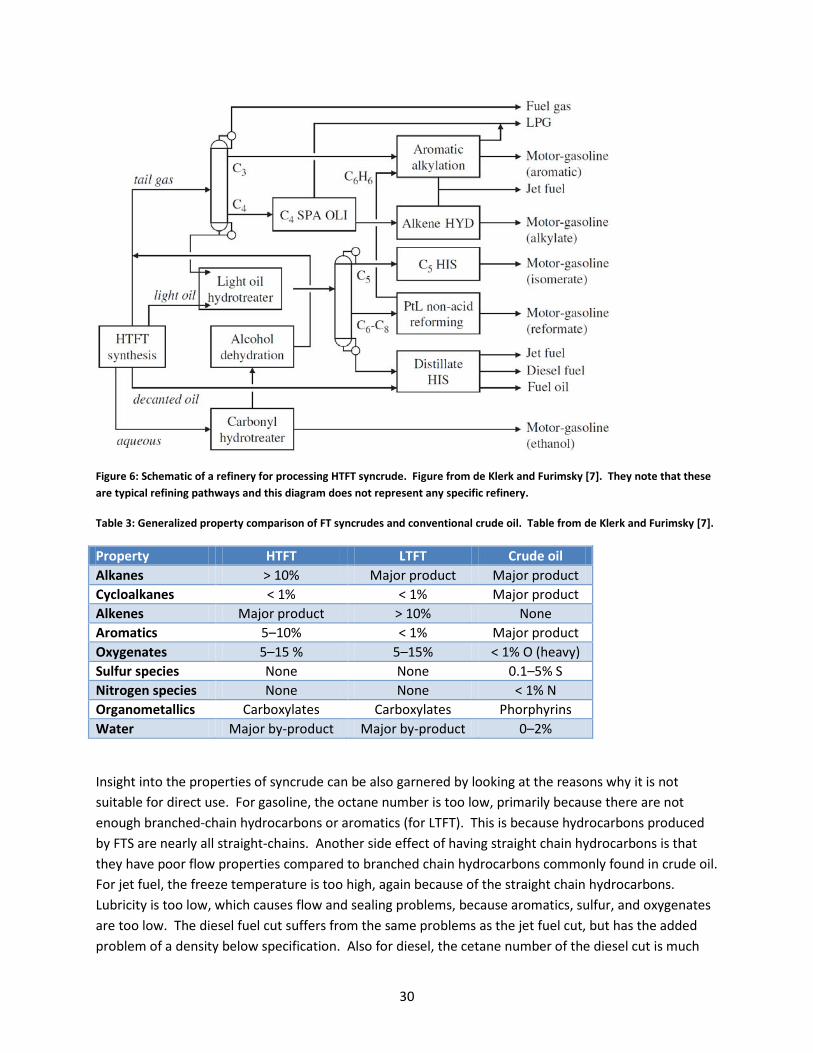
Table 3: Generalized property comparison of FT syncrudes and conventional crude oil. Table from de Klerk and Furimsky [7].

Property HTFT LTFT Crude oil Alkanes > 10% Major product Major product Cycloalkanes < 1% < 1% Major product Alkenes Major product > 10% None Aromatics 5–10% < 1% Major product Oxygenates 5–15 % 5–15% < 1% O (heavy) Sulfur species None None 0.1–5% S Nitrogen species None None < 1% N Organometallics Carboxylates Carboxylates Phorphyrins Water Major by-product Major by-product 0–2%

Insight into the properties of syncrude can be also garnered by looking at the reasons why it is not suitable for direct use. For gasoline, the octane number is too low, primarily because there are not enough branched-chain hydrocarbons or aromatics (for LTFT). This is because hydrocarbons produced by FTS are nearly all straight-chains. Another side effect of having straight chain hydrocarbons is that they have poor flow properties compared to branched chain hydrocarbons commonly found in crude oil. For jet fuel, the freeze temperature is too high, again because of the straight chain hydrocarbons. Lubricity is too low, which causes flow and sealing problems, because aromatics, sulfur, and oxygenates are too low. The diesel fuel cut suffers from the same problems as the jet fuel cut, but has the added problem of a density below specification. Also for diesel, the cetane number of the diesel cut is much

31

Table 4: Commonly used crude oil refining technologies and catalysts, and their compatibility with FT syncrude. Neutral and Good indicate possible efficient use in FT syncrude refining, while Poor indicates some inefficiency. Table from de Klerk and Furimsky [7].

Conversion process Main catalysts for crude oil refining

FT compatibility

Aliphatic alkylation HF Poor Aliphatic alkylation H2SO4 Poor Catalytic reforming Pt/Cl-/Al2O3-based Poor C5/C6 hydroisomerisation Pt/Cl-/Al2O3 Poor C5/C6 hydroisomerisation Pt/SO4

2- /ZrO2 Poor C5/C6 hydroisomerisation Pt/H-MOR Neutral Alkene etherification Acidic resin Neutral Alkene oligomerisation SPA Good Alkene oligomerisation ASA Good Sweetening Co phthalocyanine Irrelevant Hydrotreating Sulfided NiMoW/Al2O3 Neutral Hydrocracking Sulfided NiMoW/SiO2–Al2O3 Neutral Fluid catalytic cracking USY Poor Visbreaking of residue No catalyst Irrelevant Coking No catalyst Poor

higher than that required by the specification. While this may cause poorer emissions, the more important issue is in the wasted value of the “extra cetane” that is not required. These issues with syncrude can be solved by proper processing (refining), blending with crude oil, blending with finished product, or a combination of these.

The reader is now also likely to appreciate that the most efficient design of a syncrude refinery will depend on the type of FT reactor being used and the desired product. The focus of liquid fuel production by Fischer-Tropsch Synthesis is often on the FTS unit itself, which in many people’s minds makes that the first and most important element to be specified. In fact, it seems that design of a successful synthetic fuels plant based on FTS should consider the FTS unit as just another reactor in the many steps to go from syngas to saleable product. Once this mentality is established, design tradeoffs between the FTS unit and the other components become evident and the most efficient overall plant to produce a desired product can be determined.

Another implication of this discussion is that if product flexibility is desired, it is likely to come at a cost of decreased operating efficiency or, at best, increased capital cost.

2.5 Current Facilities Table 5 summarizes the known, commercial Fischer-Tropsch facilities that exist today and in the recent past. Pictures of some of these facilities are shown in Figure 7 through Figure 13.

32

The most well-known and successful companies to apply FTS on a commercial level are Sasol and Shell and their achievements in the field are evidenced by the number and scale of their operating plants as shown in Table 5. Other smaller, less renowned companies and ones that do not currently have commercial facilities are described in more detail below.

Rentech uses Fe-LTFT SBC technology and has a 7-10 bbl/day demonstration unit running in Commerce City, CO on natural gas and petroleum coke, producing primarily jet and diesel fuels. Rentech has plans to install a biomass gasifier at the site and test biomass-derived syngas feedstock as well. The company has a plan for a larger biomass-to-liquids plant in White River, Ontario (Canada) with a capacity of about 1,800 bbl/day of finished fuels, and a less-defined plan of a mixed feed (biomass, coal, natural gas) plant with carbon sequestration in Adams County, Mississippi. The proposed output is about 28,000 bbl/day, primarily jet fuel, although it is not clear how much of this is intended to come from the FTS unit(s).

Syntroleum is on a smaller-scale and has been involved in technology development since 1984, but currently the only FT plant in operation is a demonstration unit in Zhenhai, China. They have long been known to be interested in developing a FT unit mounted on a barge that could be easily moved to exploit stranded natural gas resources that are too small to be considered viable for traditional extraction and processing methods, but this has not yet been realized.

Synterra is building a biomass-to-liquids (BTL) plant at the University of Toledo (Ohio) that plans to use gasified woody biomass and rice hulls as the input to the FTS unit to produce 20 bbl/day crude oil equivalent.

There are several other small-scale companies developing FT reactor technologies. Velocys (part of Oxford Catalysts Group) has developed a microchannel reactor that is supposed to greatly increase the heat transfer and therefore increase the efficiency and reduce the size of the reactor. A picture can be seen in Figure 14. They have demonstrated their technology with gasified wood chip feedstock for six months in 2010 at Gussing, Austria. A picture of the facility is in Figure 15.

Chart Energy & Chemicals has developed two types of compact heat exchange reactors that are applicable for FTS. The reactors have been tested at the University of Kentucky with 100 µm catalyst particles, but the commercial status is unknown.

Ceramatec has developed what they claim to be a compact FT reactor, marketed as transportable. The fixed-bed tubular reactor is 0.5 m x 0.5 m and 2 m long and produces about 1-2 bbl/day. It has undergone successful testing but the commercial status is unknown.

33

Table 5: Summary of commercial FT facilities

Name Location Majority Owner

Dates (Full production)

FT Technology Feedstock FTS Production Volume*

Primary Product

Sasol 1 Sasolburg, So. Africa

Sasol 1955 - current

Fe-HTFT CFB, (decommissioned in 1990’s); Fe-LTFT SBC (1990’s to current); in parallel with Fe-LTFT fixed bed (entire time)

Coal until 2005, converted to natural gas

6,750 bbl/day (original)

Gasoline (initial design), now waxes and chemicals.

Sasol 2 and Sasol 3 Secunda, So. Africa

Sasol Sasol 2: 1980 - current; Sasol 3: 1983 - current

Initial: Fe-HTFT CFB; Converted to Fe-HTFT FFB in 1995

Coal 120,000 bbl/day

Gasoline

Mossgas Mossel Bay, So. Africa

PetroSA 1993 - current

Fe-HTFT CFB Natural gas 24,000 bbl/day

Gasoline and Diesel

Shell Bintulu Bintulu, Malaysia

Shell 1993 - current

Co-LTFT fixed bed Natural gas 12,000 bbl/day

Distillate

Pearl GTL Ras Laffan, Qatar

Shell 2011 - current

Co-LTFT fixed bed Natural gas 140,000 bbl/day

Distillate

Oryx GTL Ras Laffan, Qatar

Qatar Petroleum

2007 - current

Co-LTFT SBC Natural gas 34,000 bbl/day design, 24,000 bbl/day as of 2008

Distillate

34

Name Location Majority Owner

Dates (Full production)

FT Technology Feedstock FTS Production Volume*

Primary Product

Escravos GTL Escravos, Nigeria

Chevron Nigeria

2013 (expected)

Co-LTFT SBC Natural gas 34,000 bbl/day design

Distillate

Sinopec/Syntroleum Demonstration Facility

Zhenhai, China

Sinopec and Syntroleum

2011 Unknown (Syntroleum licenses SBC and fixed bed technologies with proprietary catalysts)

Coal, coke, asphalt

80 bbl/day Chemicals

Syntroleum Catoosa Demonstration Plant

Catoosa, OK

Syntroleum 2003 - 2006 SBC Natural gas 70 bbl/day Diesel for blending

Rentech PDU Commerce City, CO

Rentech 2008 - current

Fe-LTFT SBC Natural gas and petroleum coke

7-10 bbl/day Jet and diesel

*Production volume numbers given as crude oil equivalent and only include product made by the FT process.

35

Figure 7: Sasol 1, in Sasolburg, So. Africa. Original design of 6,750 bbl/day crude oil equivalent. Currently using Fe-LTFT SBC and Fe-LTFT fixed bed reactors with natural gas feed.

Figure 8: Sasol 2 & 3, in Secunda So. Africa. 120,000 bbl/day crude oil equivalent from coal, currently via Fe-HTFT FFB units, primary product is gasoline.

36

Figure 9: Mossgas GTL in Mossel Bay, So. Africa. 24,000 bbl/day crude oil equivalent, primary products of gasoline and diesel, natural gas feed, using Fe-HTFT CFB reactors.

Figure 10: Shell Pearl in Ras Laffan, Qatar. 140,000 bbl/day crude oil equivalent from the two Co-LTFT fixed bed units. Primary product is distillate.

37

Figure 11: Oryx GTL in Ras Laffan, Qatar. Designed for 34,000 bbl/day crude oil equivalent from natural gas, using Co-LTFT SBC reactors. Primary product is distillate.

Figure 12: Syntroleum Catoosa demonstration plant. 70 bbl/day crude oil equivalent with two SBC reactors and natural gas feed. The plant was decommissioned in 2006. The primary product was diesel for blending.

38

Figure 13: Rentech’s Product Demonstration Unit in Commerce City, CO. It uses the “Rentech reactor,” a Fe-LTFT SBC technology to produce 7-10 bbl/day crude oil equivalent. The unit is a test bed so feedstock is currently natural gas or petroleum coke and the products are primarily jet fuel and diesel.

Figure 14: Velocys microtubular reactor.

39

Figure 15: Velocys demonstration unit at Gussing, Austria, in 2010.

41

3 Fischer-Tropsch Research This chapter briefly describes the origins of FTS and then delves into the current literature. The latter is separated into three parts: literature related to reactor design, experiments, and modeling.

3.1 Origins The German inventors Franz Fischer and Hans Tropsch applied for a U.S. patent titled, “Process for the Production of Paraffin-Hydrocarbons with More Than One Carbon Atom” [12] in April 1926, less than a year after they applied for a similar patent in Germany and in the same timeframe that they applied for companion patents in Britain, Canada, and France. However, research (as indicated by patents) covering the conversion of carbon monoxide and hydrogen over a catalyst to form hydrocarbons had been going on for at least 20 years prior (see [13] and [14]). Thus, while 1925 or 1926 can be argued as the beginning point for research and application of the “Fischer-Tropsch” process, the concept is perhaps 20 years older than this indicates.

Figure 16 shows the approximate number of archived English literature records containing the phrase “Fischer Tropsch” from 1925 to 2011 along with selected historical dates significant to liquid fuel production and supply. The relationships to the historical events can readily be interpreted by the reader, although the small “bump” from 1945-1955 deserves some additional explanation.

In late 1943 it was realized that, as officially stated in mid-1944: “In spite of meager supplies of crude oil, the Axis has continued to find quantity and quality of such petroleum products, presumably in large

Figure 16: Number of archival publications containing the phrase “Fischer Tropsc h” since 1925.

42

degree through synthetic operations.” Thus was formed the Technical Oil Mission, an activity for “obtaining technical instruction on questions of interest to the petroleum industry in this country from conquered enemy countries.” The Mission was considered very successful in a wide variety of areas. Specifically for Fischer-Tropsch Synthesis, it obtained, “Very complete information … from a Number of commercial plants for synthesizing petroleum products By this process. The products made and described run from the Lightest ends through gasolines, kerosines, diesel oils, lubricating Oils and waxes.”1

Thus the increase in the literature in the decade following the war is most likely due to the dissemination of the Technical Oil Mission findings as well as the resulting innovation and insight in academia and industry.

3.2 Current The literature in this section is divided into three categories: reactor design, experiments or demonstrations of FTS, and modeling of the FTS process. However, there are many citations which overlap one or more of these categories so the categories should be thought of as guides rather than strict divisions.

3.2.1 Reactor Design The historical review of FTS reactors by Davis [2] contains descriptions of reactor designs from 1929 to the present. It is easy to get the impression of continual improvement in production efficiency and focus on larger and larger production facilities. For the present work, some of the more valuable portions of this piece are the innovative designs of the past that have long been ignored because of scaling problems or inefficiencies, but may be quite suitable for the goal of mobile, distributed GTL stations. As an example of this, Cornell and Cotton [16] describe a horizontal fixed-bed reactor. The advantages of this design are that it is compact (does not require a tall tower) and has an internal gas recirculation method. The gas recirculation helps to maintain isothermal conditions without the external piping or compressors needed in traditional style reactors. While this design is not readily scalable to the 10’s of thousands of barrels per day typical of the large plants of today [2], it is suitable for smaller scale operations and on its surface could be an attractive option for a mobile biomass GTL platform.

The work of Henry and Gilbert [17] provides an example of an earlier model of a trickle-bed reactor, and it relates catalyst activity and conversion to flow properties. The content of the paper suggests that to achieve wetting of an entire catalyst bed (i.e., to prevent liquid bypassing the catalyst by flowing along the walls) the Reynolds number for liquid flow should be greater than 10. The paper also notes that there is a minimum reactor length (height) required to prevent backmixing which is a function of the Peclet number and the initial and final concentrations of the products.

1 Quotes from Ref. [15] A. E. Miller, "The Story of the Technical Oil Mission," presented at the Twenty-fifth Annual Meeting of the American Petroleum Institute, Chicago, IL, November 14, 1945., available at http://www.fischer-tropsch.org/Tom%20Reels/hist_tom.htm

43

Guettel and Turek [18] model four different reactor types (fixed bed, slurry bubble column, monolith loop, and micro-structured) with a pseudo-homogeneous one-dimensional (no axial mixing) approach. They conclude that monolith loop reactors can approach slurry bubble column production capability while maintaining the advantages of a fixed bed configuration, and that micro-structured reactors achieve very high efficiencies but suffer from low productivity per unit volume. Furthermore, about 90% of the efficiency losses in a fixed bed reactor result from mass transfer limitations – about half from within the particles and half from the flow through the bed. Although the authors state that their simulation of the fixed bed may not be reliable, it still gives a qualitative indication of the importance that these mass transfer effects have on reactor performance.

Dry [10] contains an overview of the advantages and disadvantages of the four possible catalyst materials for FTS: Fe, Ni, Co, and Ru. Nickel is not recommended because of its high methane selectivity. Metal cost is given in terms relative to Fe: Co costs about 230 times, and Ru about 31,000 times. However, Co catalyst can often use less loading, reducing the practical cost (to about 10 times that of iron in one example). Ru has very high wax selectivity (88% vs 60% for Fe) and may be viable for smaller plants where a higher cost product can be justified. However, Ru worldwide supply would be an issue if it was to be used in significant amounts. Neither Co nor Ru oxidize or deposit carbon during normal FTS operating conditions, which is an advantage over Fe which oxidizes to inactive iron oxide (this is in contrast to Madon and Taylor [19] which states that iron oxide can still be active in FTS) and whose carbon deposition can block active sites and lead to catalyst swelling (not so much of a problem for lower temperature operation (< 270 °C), though). It also notes that all catalysts are permanently poisoned by sulfur, and that Sasol reduces sulfur content to < 0.05 ppm for the inlet gas. Therefore, if the bed is subjected to sulfur, then the longer life and better performance of Co compared to Fe cannot be realized and the extra cost is wasted.

The measurements show that peak activity of a Fe catalyst in a fixed bed tubular reactor occurs at approximately 1/3 the reactor length, while the wax selectivity peak occurs close to the exit. Both parameters experience a decrease over time. The decrease of activity near the inlet was attributed to sulfur poisoning, while that near the outlet was attributed to particle sintering and subsequent area loss. Regarding the sulfur effect, it is not because the back of the bed is somehow more resistant to sulfur, it’s just that most of it has already been adsorbed by the front of the bed (although it is noted that some sulfur compounds may be adsorbed more readily than others, meaning some compounds could penetrate deeper into the bed before adsorption. And the sintering is due to oxidation by H2O (hydrothermal sintering) which increases as more H2O is produced along the bed length.

In studies of Fe catalyst particles used in high temperature fluidized bed operation, it was found that the cores of larger particles were transformed to iron oxide. The hypothesis presented is that as the syngas travels deeper into the particle, it becomes converted along the way and as a result more H2O is produced. At the core the high concentration of H2O leads to oxidation.

The concept of liquid holdup often measured in fluid flow studies of reactors but rarely explained, is defined in detail by de Klerk [20], including the definition of related concepts.

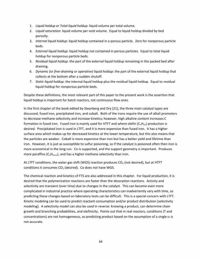
44

1. Liquid holdup or Total liquid holdup: liquid volume per total volume. 2. Liquid saturation: liquid volume per void volume. Equal to liquid holdup divided by bed

porosity. 3. Internal liquid holdup: liquid holdup contained in a porous particle. Zero for nonporous particle

beds. 4. External liquid holdup: liquid holdup not contained in porous particles. Equal to total liquid

holdup for nonporous particle beds. 5. Residual liquid holdup: the part of the external liquid holdup remaining in the packed bed after

draining. 6. Dynamic (or free-draining or operative) liquid holdup: the part of the external liquid holdup that

collects at the bottom after a sudden shutoff. 7. Static liquid holdup: the internal liquid holdup plus the residual liquid holdup. Equal to residual

liquid holdup for nonporous particle beds.

Despite these definitions, the most relevant part of this paper to the present work is the assertion that liquid holdup is important for batch reactors, not continuous flow ones.

In the first chapter of the book edited by Steynberg and Dry [21], the three main catalyst types are discussed, fused iron, precipitated iron, and cobalt. Both of the irons require the use of alkali promoters to decrease methane selectivity and increase kinetics; however, high alkaline content increases C formation in fused iron. Fused iron is mainly used for HTFT and where olefin (CnH2n) production is desired. Precipitated iron is used in LTFT, and it is more expensive than fused iron. It has a higher surface area which makes up for decreased kinetics at the lower temperature, but this also means that the particles are weaker. Cobalt is more expensive than iron but has a better yield and lifetime than iron. However, it is just as susceptible to sulfur poisoning, so if the catalyst is poisoned often then iron is more economical in the long run. Co is supported, and the support geometry is important. Produces more paraffins (CnH2n+2), and has a higher methane selectivity than iron.

At LTFT conditions, the water gas shift (WGS) reaction produces CO2 (not desired), but at HTFT conditions it consumes CO2 (desired). Co does not have WGS.

The chemical reaction and kinetics of FTS are also addressed in this chapter. For liquid production, it is desired that the polymerization reactions are faster than the desorption reactions. Activity and selectivity are transient (over time) due to changes in the catalyst. This can become even more complicated in industrial practice where operating characteristics can inadvertently vary with time, so predicting these changes based on laboratory tests can be difficult. This is a special concern with LTFT. Kinetic modeling can be used to predict reactant consumption and/or product distribution (selectivity modeling). A selectivity model can also be used in reverse: knowing a product, can determine chain growth and branching probabilities, and olefinicity. Points out that in real reactors, conditions (T and concentrations) are not homogeneous, so predicting product based on the assumption of a single α is not accurate.

45

Chapter 2 of the book edited by Steynberg and Dry [22] considers the design of and issues with FT reactors.

Liquid condensation of C5+ product occurs when T < 329 °C. LTFT reactors operate in the 220 °C to 250 °C range. Design recommendations for fixed bed reactors include:

1. Small diameter (e.g., ≅ 5 cm diameter), catalyst containing tubes with high gas linear velocities for turbulent flow, surrounded by coolant to approach isothermal conditions as close as possible.

2. Recycle tail gas (for higher gas velocity without too much compromise in production) and liquid (for better heat conductivity), both with the goal of maintaining isothermal conditions. Notes that anytime there is gas recycle, “it goes without saying” that the gas is first cooled to condense out any water and product before it is recycled. High conversion (> 90%) can be achieved by multiple reactors in parallel feeding into a single reactor (with liquid condensation between), as used by Shell at their Bintulu plant.

3. Particle size ≥ 1 mm to avoid unacceptable pressure drop and destruction of the particle, and give better heat transfer, although smaller particles would give a better productivity.

4. Iron based reactors typically have large axial temperature gradients because most of the reaction occurs at the inlet.

5. Higher pressure gives more yield with no change in product distribution.

The effect of liquid overall is to increase pressure drop and enhance heat transfer, although the effects are small. A typical liquid velocity is 1 mm/s for the downflow trickle bed. The biggest effect of liquid is to fill the catalyst pores, inhibiting diffusion (among other concerns addressed in other papers).

High temperature leads to more methane selectivity, C formation, and catalyst damage. Tube and catalyst dimensions are designed to deal with or reduce the peak possible temperature, which means that most of the reactor is overdesigned.

A successful model must have some kind of single particle model to account for the effect of intraparticle diffusion limitations on productivity and selectivity. The thermal conductivity of the liquid/wax within pores is important. The convective heat transfer coefficient at the wall at static conditions is an important unknown and complicated by voidage at the wall.

Attributes differences in theoretical and measured diffusivities within particles to porosity/tortuosity effects. (However, unless this took into account the actual diffusion through liquid/wax build-up the calculated porosity/tortuosity would be in error). Hollow, eggshell-like particles can be used to get better heat transfer, lower pressure drop, and are possibly cheaper, but they are not as mechanically robust. This may be an option for smaller beds where the weight they need to support is smaller.

General H2 feed staging options were discussed by Guillou et al. [23], analyzed with an empirical model, and tested in a wall-coated catalyst microchannel reactor. The results showed that H2 staging could reduce C1-4 selectivity and increase C5-9 selectivity. Although separating the H2 for staging may not be

46

desirable for a compact bio-syngas reactor, the work provides an example of the kind of ideas that could be examined.

3.2.2 Experiments Saroha and Khera [24] test trickle bed reactors in two different flow configurations (co-current upflow and co-current downflow) to compare the pressure drop, liquid holdup, and axial dispersion (mixing). This work shows that upflow may have similar characteristics to downflow when the flow is high enough, and for smaller scale reactors. Even at higher velocities, upflow consistently has more axial mixing than downflow. This means that upflow may be advantageous because it typically has more mixing which would result in increased heat transfer. This work also contains detailed information about the experimental apparatus.

Post et al. [25] contains experimental data on the performance of different catalyst materials (Fe or Co based) with varying size and pore diameters with the main goal of quantifying diffusion limitations. For iron, productivity increases with decreasing particle diameter. This is postulated to be because of strong diffusion limitations within the particle. The effect of diameter is stronger for catalysts with lower porosity and average pore diameter. For the Co catalyst study, calculations of hydrogen diffusivity derived from the data correspond to the theoretical diffusivity for hydrogen through a heavy paraffinic liquid (molecular weight 300-400 kg/kmol; e.g. C22 – C28) and it was shown that the diffusivity is independent of pore size. The method used in the paper may also be useful for quantifying diffusion in further experiments.

Niemantsverdrlet et al. [26] shows that iron catalysts undergo continual transformation into carbide during FTS. There is an activation time associated with a new catalyst exposed to syngas, where much of the CO goes into making carbides instead of hydrocarbon products. This time seems to be on the order of 5-20 hours (before the reaction becomes stable). After this time the catalyst will be nearly all converted and additional C from the CO will be deposited on the surface.

The introduction of Bukur et al. [27] contains information on the role of promoter and support additives to iron catalysts. In general, the use of support and promoter in the proper portions is essential to maximize productivity and selectivity of longer-chain products. The work contains detailed procedures on preparing the final catalyst including the pre-operational reduction. The results indicate that while the addition of silica decreases catalyst activity, the catalyst is more stable, i.e., experiences less reduction in activity over time. In addition, the addition of silica has a non- linear effect on hydrocarbon selectivity that is not understood.

Dry [28] presents an overview of Sasol operations as of the date of the paper (1990) and also a review of some experimental observations of FTS. It shows a schematic of the operation as well as details on the reactor beds. Relevant observations are: (1) Promotion of Fe catalyst with potassium (K2O) can significantly affect the product distribution, e.g. it increased the “hard wax” yield from 5% to 63%. (2) Increased temperature leads to higher selectivity of lower C products. In fact, thermodynamics analysis shows that at typical FT conditions the product should be primarily CH4 and carbon. This means that engineering the selectivity of FTS is a battle between natural thermodynamic (equilibrium) tendencies

47

and catalyst-controlled kinetic factors. (3) For LTFT using precipitated iron catalysts at 220 °C, the H2:CO ratio inside the reactor is the dominant factor in controlling selectivity; total and partial pressures have little effect. For HTFT, the opposite is true. (4) Product selectivity is determined by chain growth probability, and if each possible constituent has equal probability it means there is no way to adjust selectivity to exceed a certain percentage for anything other than the extreme ends. However, there is evidence that the probability may not be uniform, and one possible explanation is that the formation of longer chains in liquid filled pores may have a higher probability due to longer residence times caused by slower diffusion processes. (5) Fe catalyst preparation is described. It is noted that the formation of carbide during initial startup is highly exothermic and thus startup should proceed slowly (several hours). (6) Sulfur, and to a lesser extent, Chlorine will poison the catalyst. (7) It has been observed that “washing” the wax out of the pores in the catalyst increases performance but only lasts on the order of minutes before the pores are re-filled. (8) Hydrothermal sintering is crystal growth of the catalyst, reducing active surface area.

Schulz et al. [29] performed experiments on Co and Fe catalysts to determine the effects of H2, CO, and H2O partial pressures and temperature on the intrinsic kinetics of FTS. The reaction rate increases with increasing pH2, decreasing pCO, and increasing T. The effect of increasing pH2O is to decrease the reaction rate for Fe catalysts and increase it for Co catalysts. Methane production decreases with decreasing pH2, increasing pCO (the effect on Fe is small), increasing pH2O (the effect on Fe is small), and decreasing T. Product desorption is inhibited (i.e., chain growth probability increases) with decreasing pH2, increasing pCO (although for Fe the effect is insignificant), increasing pH2O, and decreasing T (the effect is dramatic). Chain branching probability was different for Co and Fe. For Fe, it decreased with decreasing pH2, increasing pCO, decreasing pH2O, and decreasing T, although the effects are small for pH2 and pCO. The notable result is that each of the conditions for increasing reaction rate are the opposite required for moving the selectivity to higher C products.

Al-Dahhan and Dudukovic [30] provide details of their experimental system for a trickle-bed reactor at high pressure. They also provide a phenomenologically-reasoned expression with empirical coefficients to determine the extent of catalyst wetting (desired for liquid-limited reactions, to be avoided for gas limited reactions such as FTS). An examination of this expression reveals that factors that increase wetting are: increased liquid flow rate, decreased bed voidage (which can be done through decreased particle size), increased pressure drop (which can be done by increasing either gas or liquid flow rate), and decreased reactor height. Higher pressure was also shown to increase wetting by increasing the pressure drop via increased gas density. Therefore, to reduce wetting (as would be desired for FTS), the desired conditions would be low flow rates, large particles, low pressure, and increased reactor height (without affecting pressure drop). More details of the experimental reactor itself are given in Khadilkar et al. [31], which compares performance of upflow and downflow modes of operation of a trickle bed. It notes that because of increased catalyst wetting in upflow, gas-limited reactions favor downflow.

The existence of CO gradients in catalyst particles is confirmed by de Jong et al. [32] which found the gradient to be accurately described by the Thiele modulus with φ = 3.45.

48

Sie and Krishna [33] show that intraparticle diffusion becomes significant for particle diameters greater than 0.5 mm. This is lower than the typical lower limit is 1 mm used to limit pressure drop in fixed bed reactors. They note that the Thiele modulus can be used to accurately model diffusion of H2 in a paraffinic liquid as long as it is corrected for pore volume and tortuosity. If the effect of water on diffusion suggested by Iglesia [34] is true, then it must mean that this correction also includes the effect of water unbeknownst to the author. The paper also gives some historical context as well as a description of the recommended approach to design and building new reactors, incorporating modeling as well as experiments.

An important experimental result related to the kinetics of the FTS reaction is that of the reaction order of hydrogen. Rather than describe each paper in detail, Table 6 summarizes the literature in this area.

3.2.3 Modeling The general scope of modeling activities on FTS are best described by Froment and Bischoff [35], which presents the types of models that are used to simulate fixed-bed behavior. The first thing to note in modeling is that even in the most basic model the reactor is divided into nodes (“discretized”) along its length, thus giving overall gradients along the axial direction. In all cases, the properties (velocity, concentration, temperature, pressure) within a node are assumed constant throughout the node, but the different methods for calculating these properties is what gives rise to the different model types.

The most basic model is the pseudo-homogenous one-dimensional model. The separate effects of catalyst and fluid on heat and mass transfer are not explicitly calculated but are lumped together and temperature and concentration are the same for both the fluid and catalyst (pseudo-homogeneous). Temperature and concentration changes (from inlet to outlet of the node) in the axial direction are considered, but not in the radial direction (one-dimensional). Concentration change is simply a function of the extent of reaction within the node. Temperature change is a function of the heat of reaction within a node and the amount of heat transferred in/out of the node in the radial direction (e.g., through the tube wall to the coolant). In the most basic form of this model, flow is assumed to be plug flow with no consideration of the velocity profile or axial gradients, but a modification to this assumption can be made by considering an effective axial mass diffusion superimposed onto the bulk plug flow, as well heat transfer in the axial direction. This referred to as pseudo-homogeneous one-dimensional model with axial mixing. The effect of axial mixing is negligible when the bed depth is more than 50-times the particle diameter, so it is often ignored.

An increased level of fidelity comes from the pseudo-homogeneous two-dimensional model, which considers concentration and temperature gradients in the radial direction (i.e., radial mixing). It is generally agreed that FTS in fixed bed reactors, especially those using iron catalysts, should be two-dimensional. This is due the large amount of heat generated (high exothermicity of reaction) and poor radial heat transfer which leads to radial temperature gradients, combined with a high sensitivity of product distribution to temperature which makes it imperative to know these gradients. The exact method of modeling radial gradients in temperature and concentration can vary, but in general the continuity and energy equations now include an additional term describing the radial flux of mass and energy, respectively. Jess and Kern [36] presents a modern model of this type.

49

Table 6: Summary of hydrogen reaction orders (experiment based)

Reference pH2 order Catalyst Reactor T and P pH2 range Notes van der Laan [37]

0.5 Precip. Fe Ruhrchemie (Fe/Cu/K/Si)

Slurry 523 K; 0.8-4 MPa

0.4 -3.5 MPa

Graph shows a (-) pH2 rxn order, but this is explained by being influenced by increasing pH2O

van Berge [38]

0.5 Sasol Arge based on Precip. Fe Ruhrchemie (Fe/Cu/K/Si)

CSTR/ slurry

523 K; 20.8 bar

1.4-15.3 bar

Statistical experiment approach – no single rFT vs. pH2 chart available

Zhou et al. [39]

0.5 Fe, proprietary

Slurry 533 K; pH2 + 0.28 MPa

0.4-2.47 MPa

Schulz et al. [29] 1994

0.5 Precip. Fe/Al/Cu/K

CSTR/ slurry

523 K; pH2 + 4 bar

3-30 bar Varying P at same time as pH2. Best fit on pH2 graph is pH2 order 0.43, but data points could also be fitted to straight line.

Dry 1 Assume Fe HTFT, LTFT (assume fixed bed)

T=?; 9.4-21.5 bar (?)

Very little details

Ojeda et al. 1 Fe/Zn/Cu/K Fixed bed

508 K; pH2 + 0.4 MPa when doing pH2 study

0.4-1 MPa Data could also be interpreted as rxn order >1

Lox and Froment [40] 1993

>1 (by graph)

Precip. Fe/Si/Cu/K/Na

Tubular fixed bed

523 K; pH2 + 0.2 MPa

0.46 – 1 bar

Tubular reactor, low pressures: may not be applicable results

Lit review in van der Laan [37]

1 or 2 Various iron Notable is that none of the Fe catalyst studies he cites use pH2 order < 1

Wang et al. [41]

0.5 for olefins, 1.5 for methane and paraffins

Precip. Fe/Cu/K

Fixed bed

493-533 K; 11-31 bar

Varies

Zhang et al. [42]

0.5-2.5 Precip. Fe/Cu/K

SBR 525 K; 0.5-1.5 MPa

Varies Pressures are a little low

The heterogeneous one-dimensional model has the same assumptions as the pseudo-homogeneous one-dimensional model, except for the fact that the fluid and catalyst properties are not assumed to be

50

the same and there are separate mass and energy equations for the fluid and solid. It should be noted that no matter how many separate aspects of the fluid and catalyst are considered, if these are used to generate a set of parameters that are used in only one set of conservation and energy equations then the model is considered pseudo-homogenous as opposed to heterogeneous. The basic version of this is the one-dimensional heterogeneous model accounting for interfacial gradients which considers separate but constant property values for the solid and fluid with a gradient only at the interface.

When gradients (concentration and temperature) within the catalyst particle are considered, the one-dimensional heterogeneous model accounting for interfacial and intraparticle gradients is used. Diffusion and heat transfer through the particle are modeled. Wang et al. [43] presents a recent model of this type. If the particle can be assumed to be isothermal, the equations simplify somewhat. This can often be assumed with negligible effect.

The two-dimensional heterogeneous model accounting for interfacial gradients is the same as the one-dimensional model discussed above except it also considers mass and heat transfer in the radial direction with the important distinction of considering the heat transfer separately for the fluid and solid. There are several examples of this model in the literature.

The most general model is a two-dimensional heterogeneous model accounting for interfacial and intraparticle gradients. A model of this type would include:

• Separate mass and energy equations for the particle and the fluid (heterogeneous). • Gradients in temperature and concentration in the radial direction (two-dimensional) for both

the fluid and the particles. • Mass and heat transfer at the boundaries between the fluid and the particle (interfacial

gradients). • Determination of concentration and temperature gradients inside the particle (intraparticle

gradients). • Axial mixing (optional).

3.2.3.1 Chemical Reactions and Kinetics Chapter 3 of the book edited by Steynberg and Dry [11] goes into detail on the FTS reactions. The simplified (overall) reactions occurring in FTS are:

a. CO + 3H2 → CH4 + H2O (methane) b. nCO + 2nH2 → (-CH2-)n + nH2O (heavier hydrocarbons) c. nCO + 2nH2 → CnH2n+2O + (n-1)H2O (alcohols) d. CO + H2O → CO2 + H2 (WGS, reversed for HTFT)

The term “conversion” refers to consumption of reactants, not production of products. Theoretically, want the inlet syngas to have a H2:CO ratio similar to that of the desired products (the usage ratio). So for liquid fuels, want H2:CO ≅ 2, and stay away from H2:CO = 3, which is what produces methane. However, because WGS steals some of the CO, the actual usage ratio in a reactor is closer to 1.65.

51

Lowering the inlet to this level will reduce the reaction rate and create the possibility for more C deposition, so more H2 is used in practice. The chain growth probability (α) seems to depend on the C-number of the product, not just on the operating condition. (Other papers address this in detail.) But it is certain that higher T typically increases methane selectivity because the desorption process is endothermic. It should be clear that α depends on the partial pressures at the reaction site as opposed to those in the bulk. This chapter also mentions the effect of liquid/wax buildup in pores, noting that plugged pores may allow for longer residence times thus increasing α inside the pores. And because H2 diffuses more readily than CO, the H2:CO ratio inside the pore may be higher than in the bulk. Addition of a promoter such as K and Na salts theoretically increases reaction rate and gives higher liquid selectivity. However, the production of more liquids may end up lowering the activity because more pores become clogged with liquid. It seems a lower concentration of CO would lead to better liquid selectivity, so this is another tradeoff between productivity and selectivity. Deviations from an ASF distribution are probably due to chain-length dependent solubilities. Futhermore, it is unlikely that olefin reincorporation is due to longer residence time in pores, as is the fundamental explanation behind the diffusion-controlled model of Iglesia et al. [44]. The kinetics of the FTS reaction are unknown and still debated in the literature. A summary of work to-date is given in Table 7. Following the table, more detailed descriptions of selected works are given.

Botes and Breman [45] look at various proposed macrokinetic rate equations and through arguments come up with an optimal expression which is ½ order in pH2, contains a vacancy term in the denominator, and assumes H2 dissociation / LHHW mechanism (squared denominator). It compares the equation to data in four other studies (summarized more clearly in Botes [46]) and finds it fits better than the equations proposed by any of the others to describe their own data, and also validates the equation based on their own experiment. The reason for choosing ½ order for pH2 is unexplained – only because of van Berge’s conclusions.

Zhou et al. compares historical classes of macrokinetic rate models looking especially at the site balance term (the denominator). They find that the denominator should be squared (indicating H2 surface dissociation-type / LHHW / surface reaction), and the importance of the vacant site term (the “1” in the den.). It is a similar, but more thorough and quantitative historical analysis than Botes [46] and ends up resulting in the same equation proposed by Botes and Breman [45]. Just as important, they show that there is very little difference between the equation they propose and an equation for molecular reaction of hydrogen (1st order denominator / Eley-Rideal-type / gas reaction of H2) in the FTS operating range of interest. So, prior studies that show the molecular hydrogen model fitting data can be “excused” for having the wrong mechanism. Note that the chosen model has pH2 as ½ order, and the explanation for this is weak: an assumption that HCO* + * dissociating to CH* and O* is the rate determining step, but without any justification. The discarded model has pH2 as first order and no explanation is given for

52

Table 7: Summary of relevant kinetic models

Reference Kinetic Model Selectivity Model Notes Botes [45, 46]

Macro Kinetic, rCO (called rFT), no direct water influence. 2nd order den. (dissociative/LHHW rxn), ½ order pH2, vacant sites

- States that Van Berge, Anderson-Dry, Ledakowicz-Nettelhoff, Satterfield-Huff, and Van Steen equations are no good. Experimentally and theoretically confirmed by Zhou [39]. Does not comment on reaction order of H2, although uses ½ order.

Botes [47] - Desorption controlled

Thoroughly reviews previous selectivity theories and models, arguing against them.

Jess and Kern [36]

Macro kinetic, rH2, water inhibited

Methane kinetic, alpha for all others

Focuses more on mass and heat transfer

Chaumette et al. [48]

- 2-alpha: one for methane, one for C2+

Not a good selectivity model, but not the point of the paper (which was heat release)

Iglesia et al. [44]

- Olefin readsorption, diffusion controlled

van der Laan [49] shows that cannot be totally due to diffusion. Dry [11] refutes as well.

Schulz and Claeys [50]

Olefin readsorption, solubility controlled

Dry [11] supports. Justified by previous work on Co, but applied to Fe (and fits data).

van der Laan and Beenackers [49]

Olefin readsorption due to an agglomeration of effects

Parameters don’t have clear physical meaning but are comprised of several physical processes bundled together.

Dry [51, 52] Macro kinetic, rCO, water inhibited

- Shown by Botes not to work.

Kim et al. [53]

Microkinetic, uses that of Wang et al. (olefin readsorption, different WGS and FTS reaction sites)

inherent Valid for their Fe-Cu-Al catalyst.

Lox and Froment [54]

Microkinetic. Carbide mechanism. No olefin reincorporation or other effects.

inherent Several other models use this as their basis.

Wang et al. [41]

Microkinetic. Olefin readsorption. Different WGS and FTS reaction sites.

inherent For iron, but references Co-derived models (Iglesia, Schulz [50]) to justify olefin reincorporation.

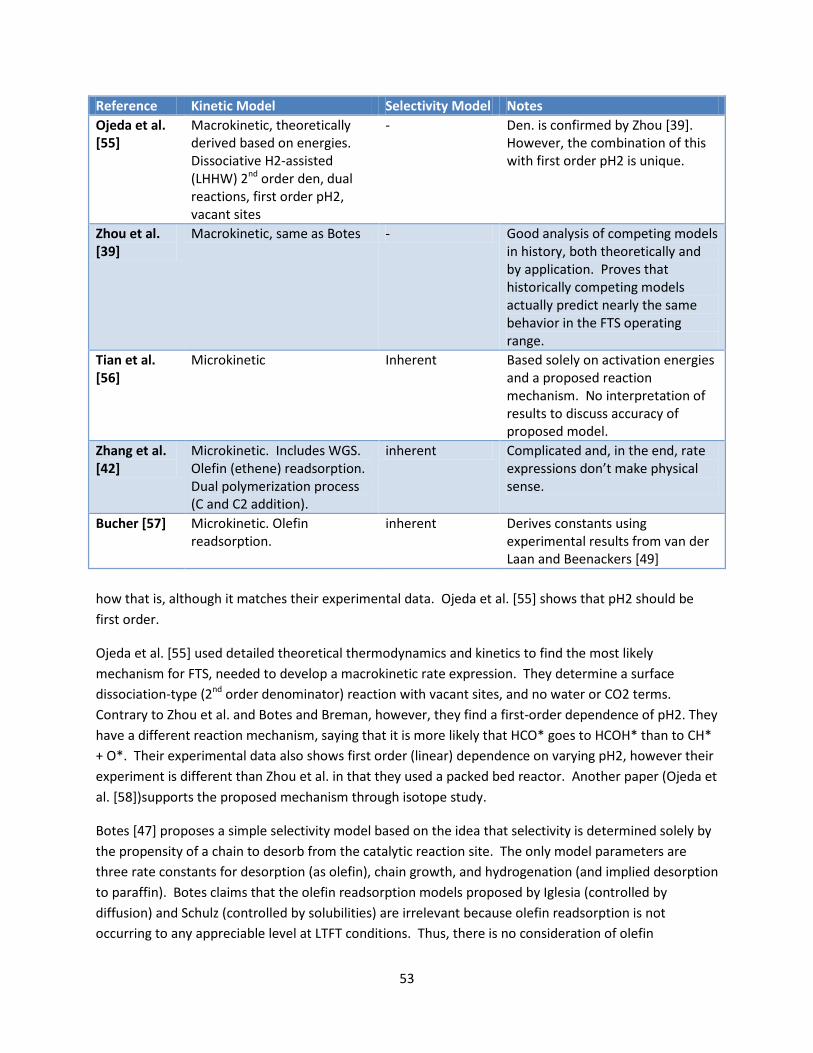
53

Reference Kinetic Model Selectivity Model Notes Ojeda et al. [55]

Macrokinetic, theoretically derived based on energies. Dissociative H2-assisted (LHHW) 2nd order den, dual reactions, first order pH2, vacant sites

- Den. is confirmed by Zhou [39]. However, the combination of this with first order pH2 is unique.

Zhou et al. [39]

Macrokinetic, same as Botes - Good analysis of competing models in history, both theoretically and by application. Proves that historically competing models actually predict nearly the same behavior in the FTS operating range.

Tian et al. [56]

Microkinetic Inherent Based solely on activation energies and a proposed reaction mechanism. No interpretation of results to discuss accuracy of proposed model.

Zhang et al. [42]

Microkinetic. Includes WGS. Olefin (ethene) readsorption. Dual polymerization process (C and C2 addition).

inherent Complicated and, in the end, rate expressions don’t make physical sense.

Bucher [57] Microkinetic. Olefin readsorption.

inherent Derives constants using experimental results from van der Laan and Beenackers [49]

how that is, although it matches their experimental data. Ojeda et al. [55] shows that pH2 should be first order.

Ojeda et al. [55] used detailed theoretical thermodynamics and kinetics to find the most likely mechanism for FTS, needed to develop a macrokinetic rate expression. They determine a surface dissociation-type (2nd order denominator) reaction with vacant sites, and no water or CO2 terms. Contrary to Zhou et al. and Botes and Breman, however, they find a first-order dependence of pH2. They have a different reaction mechanism, saying that it is more likely that HCO* goes to HCOH* than to CH* + O*. Their experimental data also shows first order (linear) dependence on varying pH2, however their experiment is different than Zhou et al. in that they used a packed bed reactor. Another paper (Ojeda et al. [58])supports the proposed mechanism through isotope study.

Botes [47] proposes a simple selectivity model based on the idea that selectivity is determined solely by the propensity of a chain to desorb from the catalytic reaction site. The only model parameters are three rate constants for desorption (as olefin), chain growth, and hydrogenation (and implied desorption to paraffin). Botes claims that the olefin readsorption models proposed by Iglesia (controlled by diffusion) and Schulz (controlled by solubilities) are irrelevant because olefin readsorption is not occurring to any appreciable level at LTFT conditions. Thus, there is no consideration of olefin

54

readsorption. While it may be reasonable to ignore olefin reincorporation at LTFT conditions, saying that selectivity is only controlled by three rate constants may be an over-simplification. For example, perhaps there is no olefin reincorporation, but without considering the effects of diffusion, solubility, or other phenomena it appears likely that the three rate constants are actually effective rate constants rather than intrinsic ones.

Wojciechowski [59] supports the assertion that olefin readsorption is unimportant at relevant Fe-based FT operating conditions. If this (olefin readsoprtion) was true, then product distributions would change over longer residence times, eventually becoming flat, which is not observed. Also notes that for data to be usable for kinetic mechanism studies, experiments must NOT be plug flow (i.e., fixed bed) design.

Cheng et al. [60] summarizes previous work on selectivity, giving an olefin/paraffin ratio calculation as well as a model for alpha. However, the references that this is based on is for Cobalt, not iron.

Kim et al. [53] has a detailed kinetic model with parameters based on their specific experiment. Contains useful definitions of selectivities.

Rahimpour et al.’s [61] model may be described as microkinetic in that it uses a separate reaction for each species. However it’s entirely empirical and lumps everything greater than C4 as C5+.

Zhang et al. [42] has a detailed microkinetic model. The uniqueness seems to come from an assumption related to the polymerization reaction – that when C<7, C is added as C2, but when C>7, C is added as C. It also incorporates olefin readsorption in the form of ethene. Haven’t seen anyone else use the double-polymerization reaction so not sure if this is valid or not.

Another important component of the kinetics of the FTS reaction is the deactivation of the catalyst over time. At constant process conditions, catalyst deactivation is the single reason for a decrease in production and/or a change in selectivity over time, and any attempt to optimize reactor lifetime must include this phenomena in its analysis. Although Moulijn et al. [62] does not specifically address FTS, the classification of causes and mechanisms of catalyst deactivation is useful. Causes are: (1) a decrease in the number of active sites, (2) a decrease in the quality of the active sites (decreasing the intrinsic rate constant), and (3) a decreased accessibility of the pore spaces. Mechanisms are:

(a) Poisoning is defined as chemisorptions on active sites of materials that are not reactants or products, and can be reversible or irreversible. It notes that poisoning can sometimes be advantageous by selectively blocking reactions that are not desired. Proper purification of the inlet stream is the obvious solution to this problem. Poisoning relates to causes (1) and (2).

(b) Fouling is any phenomenon that covers the surface with a deposit, not necessarily related to any reaction. Coke, defined as a highly hydrogen deficient carbonaceous material, is the relevant fouling problem for FTS. Coke formation in FTS is highly dependent on the temperature, catalyst, and inlet gas. Fouling relates to causes (1) and (3).

(c) Thermal degradation includes sintering (crystallization), chemical transformation, and evaporation of the catalyst particle. These processes are highly dependent on temperature and

55

can be predicted to some extent, (although most of the predictions seem empirical). Sintering relates to causes (1) and (3).

(d) Mechanical deactivation refers to loss of material or surface area due to abrasion or crushing, and is irreversible. For fixed bed reactors the primary culprits are the loading procedure and temperature transients causing stress build-ups inside the bed. Mechanical deactivation relates to cause (1).

(e) Corrosion or leaching occurs when the active catalyst dissolves into the reaction medium. It is most common in the liquid phase and is sometimes reversible. Corrosion relates to cause (1).

Not until the causes and mechanisms of deactivation are understood can steps can be taken to mitigate it. These steps include re-engineering the catalyst itself (materials and/or structure), choosing/designing an appropriate reactor (such as fixed bed vs. fluidized, or including a sacrificial catalyst layer “guard bed” at the front of the bed) and regeneration system, and customizing the operating conditions (either the design conditions or the conditions over time).

Bartholomew [63] addresses the same topic as Moulijn et al., and offers a slightly different classification system. Some of the conclusions are the same and are not repeated here, but the additional points are.

(a) Poisoning: For FTS, the main poisons are H2S, COS, As, NH3, and metal carbonyls (metal + CO). Ru, Co, and Fe all have similar tolerance to H2S poisoning, with a 103 to 104 reduction in activity for a H2S concentration of just 0.015 ppm. To combat this dramatic effect for Co and Fe, Mo and B can be added which selectively adsorb sulfur. Accurate modeling of poisoning must consider things like the fact that H2S selectively adsorbs at the entrance of the bed and on the surface of particles, and that at high pCO sulfur may be removed from surfaces as COS.

(b) Fouling and coking: Coke deposits may build up in catalyst pores, swelling or fracturing the catalyst particle. FTS is considered coke-insensitive in that it can be readily removed by hydrogen. The carbon filaments which may clog and block pores is mainly applicable only in the range of 375 °C < T < 650 °C. At T < 375 °C, a film is more likely to occur (at least, in research on Ni catalysts). This research also showed that at T < 325 °C, the rate of carbon formation was less than the rate of carbon gasification (C + H → CH) so carbon deposition is deposited. Coke in FTS can be inhibited by increasing the H2/CO ratio.

(c) Thermal degradation and sintering: Sintering typically takes place at T > 500 °C and is generally accelerated by the presence of water vapor. An empirically-fit equation (eq. 2) can be used to determine the rate of sintering for a given set of material and operating conditions. There are other (non-empirical) models available but they are typically limited in their application. There is no general model of sintering available (as of the time of the paper); perhaps this is because the author identifies no less than 12 separate mechanisms by which sintering could occur simultaneously. Sintering is inhibited when pores on the order of crystal sizes exist. Bartholomew includes solid-state reactions as a separate category. For FTS this includes transformation of active iron carbides to inactive ones.

(d) Reaction to produce an inactive phase (part of what Mouljin et al. considers a fouling mechanism, whereas Bartholomew considers fouling to not include this type of chemical

56

reaction): In FTS on Fe, (active) Fe5C2 can transform to (inactive) Fe3O4 at high CO conversion rates due to the significant presence of H2O and CO2.

(e) Corrosion and leaching (what Bartholomew refers to as reaction to produce volatile compounds): Fe can be transformed to Fe(CO)5 under high pCO at T < 300 °C. This also can apply to additives, for example loss of K in high pH2O environments.

In general, the author notes in closing that for each of the processes besides mechanical deactivation, there is still a lack of complete general mechanistic understanding (and models) and/or fundamental, intrinsic kinetic data. For mechanical deactivation, the understanding is present but so far the approaches to addressing the problem have been crude relative to the potential.

Froment [64] presents a recommended framework to model coke formation at the reaction site, on the particle, and for the reactor as a whole. For modeling reactors where coke formation is a possibility and where determinations and/or optimizations of longevity are important, this kind of analysis should be included.

Section 3 of Chapter 7 of the book edited by Steynberg and Dry [52] also addresses catalyst deactivation. Four factors given are:

1. Presence of high molecular mass waxes and/or coke precursors in the catalyst pores, resulting in diffusion restrictions. This is a fact of normal operation. Periodic washing of the catalyst bed can remove the deposits and improve performance, but only temporarily.

2. Fouling of the surface by coke deposits. 3. Poisons in the feed gas. It is noted that different sulfur compounds react with the catalyst

differently, so some could be worse than others. This means that knowing the sulfur compounds in the feed gas, not just the amount of “S,” is important. O, Cl, and Br have all been shown to poison similarly to S.

4. Hydrothermal sintering and oxidation results in oxidation of the catalyst to inactive phases (i.e., carbide to magnetite) and loss of active area by sintering. Prevalent where water concentration increases, as in deep inside catalyst pores and towards the end of the bed (since the main product of FTS is water, by far). Silica additive has been shown to retard sintering by acting as a spacer to keep grains from growing together.

3.2.3.2 Transport and Thermodynamics Jess and Kern [36] use a two-dimensional pseudo-homogeneous model without axial mixing for simulating FTS over both Fe and Co catalysts. It uses intrinsic reaction rates where possible (i.e., available in the literature). Compared to the base case which models a typical fixed-bed multi-tubular reactor, they show that increasing the radial heat transfer to the ideal situation (zero heat transfer resistance) would increase CO conversion from 32% to nearly 44% for Co catalyst.

Chaumette et al. [48] gives an expression for the enthalpy of formation of n-paraffin products that may be useful in modeling. It also simplifies the expression and provides one for the total heat generated if the product distribution α of FTS can be determined experimentally. Practically, this can be used as either a rough estimate model or as a check on a higher-fidelity model. It also includes the additional

57

heat generated by condensation of the products. While the method makes assumptions that may not be applicable to a general model, the concept is important to keep in mind even though the authors state the contribution to the overall heat generation is 2% and could be ignored.

Iglesia [34] reviews FTS using cobalt as the catalyst, but some of the findings are applicable to iron as well – but see Botes [47] for which do not (for example, olefin reincorporation and selectivity). The relevant findings are: (1) C5+ selectivity increases as CO conversion is increased by increasing reactor residence time, although the effect on C15+ is weak. (2) Chain termination probability increases with larger particles because it is more difficult for CO to diffuse to the intraparticle reaction site. (This suggests that α is a function of particle radius and probably also porosity/tortuosity, and can probably be characterized by the Damkohler number.) (3) Water, which can condense in pores at pressures below the vapor pressure because of capillary effects, is hypothesized to increase the diffusion rate of CO and H2 because both gases are more three times more diffuse in water than typical hydrocarbon products. This explains results (e.g. Shulz et al. [29]) which show that an increase in pH2O results in lower methane selectivity and inhibited product desorption. This hypothesis shows that an accurate predictive model must be able to capture the concentration gradients due to two-phase flow and diffusion with capillary effects inside the catalyst pores.

Wang et al. [43] describes a FTS, fixed bed model of the class one-dimensional heterogeneous with interfacial and intraparticle gradients with results. The introduction contains a useful review of models to-date (2003). The model is comprehensive except for the 1-D part. The contained references point to necessary sub-models such as intrinsic kinetics, mass flow, etc. Findings include (1) methane selectivity increases with temperature, (2) pressure increase leads to temperature increase, but if that is factored out then it leads to increased C5+ selectivity, and (3) gas recycle leads to better temperature distribution and a significant reduction in the hot spot at the entrance.

Philippe et al.’s [65] model is mainly focused on the transport properties. As such the kinetics are not very useful. The rate equation is empirical based on their own experiments, and the distribution is an ASF alpha model. The temperature range considered (200°C - 250 °C) is typical for Fe-based catalysts but they are modeling Co.

Cassanello et al. [66] derives a correlation from modeling results to give a threshold Peclet number above which axial mixing (dispersion) need not be considered in a model. The general idea is that a flow close to plug flow can have the axial mixing ignored.

The thermodynamic properties of FTS products can be found in the literature for C ≤ 20, and Derevich et al. [67] gives correlations for both paraffin and olefin products with C ≥ 20 for critical temperature and pressure. The group of Carl Yaws has produced numerous correlations for properties of hydrocarbons [68-82]and is used extensively in simulation of the example application of the model framework.

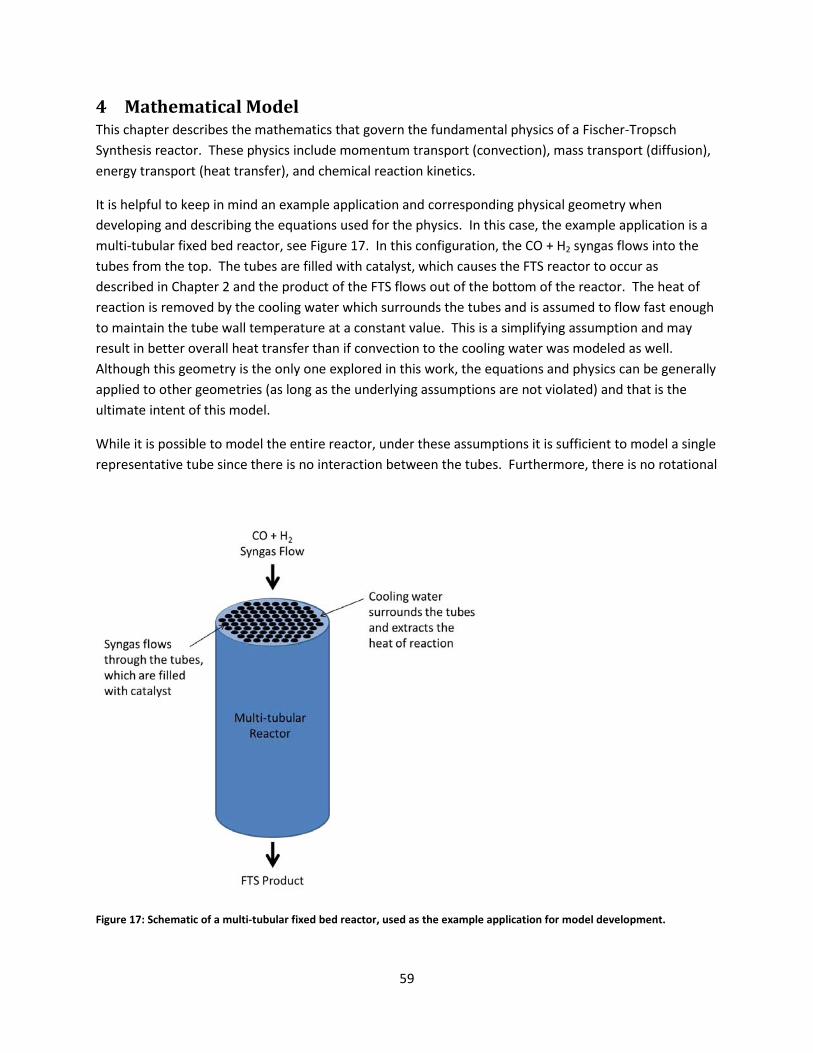
59

4 Mathematical Model This chapter describes the mathematics that govern the fundamental physics of a Fischer-Tropsch Synthesis reactor. These physics include momentum transport (convection), mass transport (diffusion), energy transport (heat transfer), and chemical reaction kinetics.

It is helpful to keep in mind an example application and corresponding physical geometry when developing and describing the equations used for the physics. In this case, the example application is a multi-tubular fixed bed reactor, see Figure 17. In this configuration, the CO + H2 syngas flows into the tubes from the top. The tubes are filled with catalyst, which causes the FTS reactor to occur as described in Chapter 2 and the product of the FTS flows out of the bottom of the reactor. The heat of reaction is removed by the cooling water which surrounds the tubes and is assumed to flow fast enough to maintain the tube wall temperature at a constant value. This is a simplifying assumption and may result in better overall heat transfer than if convection to the cooling water was modeled as well. Although this geometry is the only one explored in this work, the equations and physics can be generally applied to other geometries (as long as the underlying assumptions are not violated) and that is the ultimate intent of this model.

While it is possible to model the entire reactor, under these assumptions it is sufficient to model a single representative tube since there is no interaction between the tubes. Furthermore, there is no rotational

Figure 17: Schematic of a multi-tubular fixed bed reactor, used as the example application for model development.

60

Figure 18: A 2-D axisymmetric plane of a representative tube is the geometric basis of the mathematical model.

effect considered so that the physics within the tube can be modeled via a 2-D axisymmetric plane, as shown in Figure 18.

4.1 Governing Equations This section describes the governing (differential) equations used to model the three transport physics occurring within the reactor.

4.1.1 Mass Transport (Diffusion) Transport of liquid or gas species takes place through diffusion and bulk convection. Diffusion within each fluid phase within the reactor is handled separately.

4.1.1.1 Liquid Phase Diffusion In the liquid phase, species (i) are modeled as solutes in a dilute solution. The governing equation is:

𝜕𝑐𝑖𝜕𝑡

+ ∇ ∙ (−𝐷𝑖∇𝑐𝑖) + 𝑢�⃗ ∙ ∇𝑐𝑖 = 𝑅𝑖 (9)

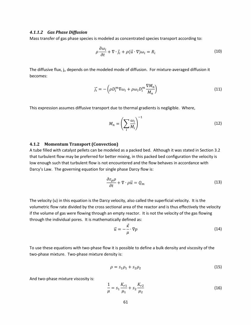
61

4.1.1.2 Gas Phase Diffusion Mass transfer of gas phase species is modeled as concentrated species transport according to:

𝜌𝜕𝜔𝑖

𝜕𝑡+ ∇ ∙ 𝚥𝑖 + 𝜌(𝑢�⃗ ∙ ∇)𝜔𝑖 = 𝑅𝑖 (10)

The diffusive flux, ji, depends on the modeled mode of diffusion. For mixture-averaged diffusion it becomes:

𝚥𝚤��⃗ = −�𝜌𝐷𝑖𝑚∇𝜔𝑖 + 𝜌𝜔𝑖𝐷𝑖𝑚∇𝑀𝑛

𝑀𝑛� (11)

This expression assumes diffusive transport due to thermal gradients is negligible. Where,

𝑀𝑛 = ��

𝜔𝑖

𝑀𝑖𝑖

�−1

(12)

4.1.2 Momentum Transport (Convection) A tube filled with catalyst pellets can be modeled as a packed bed. Although it was stated in Section 3.2 that turbulent flow may be preferred for better mixing, in this packed bed configuration the velocity is low enough such that turbulent flow is not encountered and the flow behaves in accordance with Darcy’s Law. The governing equation for single phase Darcy flow is:

𝜕𝜀𝑝𝜌𝜕𝑡

+ ∇ ∙ 𝜌𝑢�⃗ = 𝑄𝑚 (13)

The velocity (u) in this equation is the Darcy velocity, also called the superficial velocity. It is the volumetric flow rate divided by the cross sectional area of the reactor and is thus effectively the velocity if the volume of gas were flowing through an empty reactor. It is not the velocity of the gas flowing through the individual pores. It is mathematically defined as:

𝑢�⃗ = −𝜅𝜇∙ ∇𝑝 (14)

To use these equations with two-phase flow it is possible to define a bulk density and viscosity of the two-phase mixture. Two-phase mixture density is: 𝜌 = 𝑠1𝜌1 + 𝑠2𝜌2 (15) And two-phase mixture viscosity is: 1

𝜇= 𝑠1

𝐾𝑟1𝜇1

+ 𝑠2𝐾𝑟2𝜇2

(16)

62

with the liquid content s1: 𝑠1 =

𝑐1𝜌1

(17)

and: 𝑠1 + 𝑠2 = 1 (18) The determination of density and viscosity for the individual phases is described in the Constitutive Relations section. Fluid content throughout the reactor can change over time, and its movement can be tracked by an additional equation:

𝜀𝑝𝜕𝑐1𝜕𝑡

+ ∇ ∙ (−𝐷𝑐∇𝑐1 + 𝑢�⃗ 𝑐1) = 𝑓 (19)

One assumption of this equation is that porosity (εp) is constant over time. This equation tracks the liquid (fluid 1), so the source term (f) is used to represent the amount of liquid produced either directly through FTS reaction or through phase change due to pressure and/or temperature changes.

4.1.3 Energy Transport (Heat Transfer) The heat transfer physics considers the heat carried by the fluid as well as that conducted through the fluid and the porous material (catalyst). The governing equation is:

ρ𝐶𝑝𝑢�⃗ ∙ ∇𝑇 = ∇ ∙ (𝑘∇𝑇) + 𝑄 (20)

In this case the heat transfer coefficient k is an average of the heat transfer coefficients of the fluid and solid according to:

𝑘 = 𝜃𝑝𝑘𝑝 + �1 − 𝜃𝑝�𝑘 (21) Where θp is the volume fraction of the solid and is related to the porosity via:

𝜃𝑝 = 1 − 𝜀𝑝 (22) The density (ρ) is the same as that calculated for the fluid mixture by Eq. (16).

Specific heat is that of the two-phase fluid mixture. It is calculated through a phase-weighted average [83]:

𝐶𝑝 =𝜌1𝑠1𝐶𝑝,1 + 𝜌2𝑠2𝐶𝑝,2

𝜌 (23)

63

4.2 Boundary Conditions This section describes the boundary conditions of the reactor, organized by the three transport physics.

4.2.1 Mass Transport (Diffusion)

4.2.1.1 Liquid Phase At the inlet and wall, no species transport (no flux) is allowed across the boundaries. Although the inlet is a flowing boundary, this is acceptable for the liquid species because there are no liquid species in the inlet stream:

−𝑛�⃗ ∙ 𝑁𝚤��⃗ = 0 (24)

At the reactor exit, species concentration is assumed constant across the boundary, so diffusion is set to zero and the only transport is by convection:

−𝑛�⃗ ∙ 𝐷𝑖∇𝑐𝑖 = 0 (25)

Axial symmetry is applied at the r=0 boundary.

4.2.1.2 Gas Phase At the inlet, the inflow boundary condition specifies the mass fraction of each species entering the reactor:

𝜔𝑖 = 𝜔0,𝑖 (26)

Along the wall, no species transport is allowed:

−𝑛�⃗ ∙ 𝑁𝚤��⃗ = 0 (27)

At the reactor exit, species concentration is assumed constant across the boundary, so diffusion is set to zero and the only transport is by convection:

−𝑛�⃗ ∙ 𝜌𝐷𝑖𝑚∇𝜔𝑖 = 0 (28)


4.2.2 Momentum Transport (Convection) At the inlet, a uniform Darcy velocity with magnitude U0 is specified:

−𝑛�⃗ ∙ 𝜌𝑢�⃗ = 𝜌𝑈0 (29)

At the tube wall, the boundary condition specifies no momentum flux (no flow) across the boundary:

64

−𝑛�⃗ ∙ 𝜌𝑢�⃗ = 0 (30)

Note that the Darcy Law bulk flow velocity profile is plug flow in the bulk and does not incorporate a no-slip wall boundary condition.

At the exit of the reactor, the pressure is specified:

𝑝 = 𝑝𝑒𝑥𝑖𝑡 (31)

For the transport of fluid content, the inlet boundary condition is the Dirichlet type, with the amount of liquid at the inlet set to zero:

𝑐1 = 0 (32)

The wall and outlet have the same boundary condition, where the flux remains constant across the boundary:

𝑛�⃗ ∙ 𝐷𝑐∇𝑐1 = 0 (33)

This does not allow flow to cross the wall because it is implemented in conjunction with Eq. (30) which creates a no-flow condition. However, because flow is allowed to cross the outlet boundary, at the outlet this boundary condition also allows the fluid content to leave the reactor without any change.

For both transport of both momentum and fluid content, the axial symmetry condition is applied at r=0.

4.2.3 Energy Transport (Heat Transfer) At the inlet, the CO + H2 syngas flowing into the reactor is assumed to be at a set temperature. At the corner where the inlet boundary meets the wall boundary, a discontinuity will arise if the inlet and wall temperatures are different. Furthermore, in an actual reactor, it is reasonable to assume that the inflowing gas prior to reaching the packed bed will have been in contact with the wall long enough to have achieved the wall temperature uniformly. Therefore, the inlet gas temperature is set to that of the wall.:

𝑇𝑖𝑛 = 𝑇𝑤𝑎𝑙𝑙 (34)

At the wall, the temperature is specified to be that of the cooling water, which assume infinite heat transfer coefficients at the bed-wall interface, through the wall, and at the wall-water interface:

𝑇𝑤𝑎𝑙𝑙 = 𝑇𝑐𝑤 (35)

65

At the exit, the only heat transfer is by convection, so the temperature gradient in the normal direction is zero:

−𝑛�⃗ ∙ (−𝑘∇𝑇) = 0 (36)


4.3 Initial Conditions This section describes the initial conditions of the reactor for the three transport physics.

4.3.1 Mass Transport (Diffusion) In the liquid phase species are set close to zero initially (ci = 0.01). They are not set exactly to zero because this causes problems initializing model. In the gas phase the initial species concentrations are set equal to that of the inlet:

𝜔𝑖𝑛𝑖𝑡𝑖𝑎𝑙,𝑖 = 𝜔0,𝑖 (37)

4.3.2 Momentum Transport (Convection) Initially, pressure within the reactor is set to that of the outlet boundary condition, pexit.

𝑝 = 𝑝𝑒𝑥𝑖𝑡 (38)

The fluid content 1 (liquid) is set as a nearly to zero, with s1,initial in the following equation equal to 0.01:

𝑐1 =𝑠1,𝑖𝑛𝑖𝑡𝑖𝑎𝑙

𝜌 (39)

Setting exactly to zero causes initialization problems.

4.3.3 Energy Transport (Heat Transfer) Initially the temperature is set to a constant throughout the bed:

𝑇 = 𝑇𝑏𝑒𝑑 (40)

4.4 Chemical Reaction and Kinetics This section presents the mathematics used to model the chemical reactions and associated kinetics that occur within the reactor.

4.4.1 The Fischer-Tropsch Synthesis Reactions The reaction of central importance is that of Fischer-Tropsch Synthesis. As explained in Section 2.1, the FTS reaction is commonly represented by:

CO + 2H2 -> -CH2- + H2O (41)

66

The rate of consumption of CO, rCO is widely referred to as the Fischer-Tropsch reaction rate, rFT, and that convention is followed here. There is ongoing debate in the community about the best ways to represent rFT. In this study the findings of Botes [45-47, 84] are used as the basis (see the literature review section, Section 3.2.3.1 and Table 7, for more background). Based on theoretical arguments as well as strong comparisons to other workers’ experimental data, Botes proposed the following expression for rFT:

𝑟𝐹𝑇 = 𝐴

𝑃𝐻20.5𝑃𝐶𝑂

(1 + 𝑘𝐶𝑂𝑃𝐶𝑂)2 (42)

Distinguishing features of this expression are:

• Absence of dependence of H2O and CO2 on the reaction rate, implying that reaction inhibition by these species is negligible. Botes argues convincingly in favor of this perhaps contentious feature, and it is backed up by his comparisons to experimental data of a wide range of researchers as well as independently confirmed by Zhou et al. [39].

• 0.5 reaction order of H2. This is a function of the rate determining step. It has empirical basis, and is consistent among many researchers as shown in Table 6 in Section 3.2.2.

• 1 in the denominator indicates vacant sites present on the reaction surface. • The squared denominator indicates a dissociative LHHW (surface) reaction for H2. Consensus

among researchers is building in favor of the last two points.

Botes’ expression was fit to intrinsic rate experiments by Zhou et al., resulting in the following expression and constants:

𝑟𝐹𝑇 = 𝑘𝐹𝑇

𝑐𝐻20.5𝑐𝐶𝑂

(1 + 𝑘𝐶𝑂𝑐𝐶𝑂)2 (43)

To get rFT with units [mol/(gcat*s)], kFT = 4.079*10-7 and kCO = 0.106. These constants are valid for the experimental conditions of:

• Iron-based catalyst (proprietary details). • Conditioned with syngas at a H2:CO ratio of 1.6 for 250 hr. • T = 260 °C. • 10 bar ≤ P ≤ 30 bar • 0.8 ≤ Inlet H2:CO ratio ≤ 3.2

Unfortunately, there is no published literature on the dependence of kFT in this expression with temperature, so results using this expression will reflect this limitation. However, the model framework allows easy substitution of more robust expressions for these kinetic expressions.

The reaction rate for the paraffin reactions:

67

nCO + (2n+1)H2 -> CnH2n+2 + nH2O (44) is given by:

𝑟𝐶𝑛𝐻2𝑛+2 = 𝑟𝐹𝑇𝛼𝑛−1 (45) This gives a theoretical Anderson-Schulz-Flory (ASF) distribution of products as illustrated in Figure 2 and Figure 3 in Section 2.2. Modeling deviations to the ASF distribution as well as productions of olefins (CnH2n) can be accomplished within this framework by changing the constant α used here to a species-dependent α as illustrated by Botes [47] and the references contained therein.

4.4.2 The Water Gas Shift Reaction The water-gas shift (WGS) reaction is significant in low temperature FT reactors utilizing iron catalysts, which is the example application for this model, and is:

CO + H2O <-> CO2 + H2 (46) There are many models of WGS reaction rate on Ni catalyst, but for Fe catalyst the choices are limited. However, the model of Lox and Froment [54] is well-accepted and is used here for the WGS reaction rate (rCO, commonly denoted as rWGS) on Fe, and is expressed as the following when written in terms of species concentrations:

𝑟𝑊𝐺𝑆 = 𝑘𝑣(𝑅𝑇)1.5�𝑐𝐶𝑂𝑐𝐻2𝑂𝑐𝐻20.5 − 1

𝐾𝑒𝑤𝑔𝑐𝐶𝑂2𝑐𝐻2

0.5�

�1 + 𝐾𝑣(𝑅𝑇)0.5 𝑐𝐻2𝑂𝑐𝐻20.5 �

2 (47)

To get rWGS with units [mol/(gcat*s)], kv = 5.57*10-5 and Kv = 3.6. Kewg is a function of temperature:

𝐾𝑒𝑤𝑔 = 𝑒𝑥𝑝[5078.0045/𝑇 − 5.8972089 + (13.958689 ∗ 10−4)𝑇− (27.592844 ∗ 10−8)𝑇2]

(48)

In both equations, T must be in [K] and the concentrations used are those of the gas phase. These constants are valid for the experimental conditions of [40]:

• Precipitated iron catalyst, stabilized with SiO2 and promoted with K2O and CuO. • Reduced with H2 and stabilized in a syngas atmosphere with a H2:CO ratio of 2 for 12 hours. • 250 °C ≤ T ≤ 350 °C. • 6 bar ≤ P ≤ 21 bar • 3 ≤ H2:CO molar feed ratio ≤ 6

4.4.3 The Phase Change Reactions The final reactions of importance are the phase change reactions. In Eq. (43) it can be seen that the amount of product species does not influence the FT reaction rate. Therefore, the phase of the product

68

species phase has no impact on its production rate either. This fact can be used to ignore determining the product phase in the chemical kinetics of the FT reaction which makes implementation of the reaction scheme easier.

The exception to this is water, with respect to the WGS reaction rate. A choice must be made on which phase of water to allow to participate in the reaction. Fortunately, Davda et al. [85] showed that the WGS reaction occurs entirely with gas-phase water when the other reactants are gasses. Even when the catalyst is submerged in liquid water, the gas bubbles of the other reactants are what reacts and those gas bubbles contain water vapor at saturation. Therefore, in this work only gas phase water is allowed to participate in the WGS reaction. For this reason, knowledge of the phase of water and amount of gaseous water at a given point in the reactor is necessary.

Determination of the phases of the product species is critical as well because of the effect on the thermal and fluid mechanical properties of the two-phase mixture flowing through the reactor. Also the heat of vaporization must be factored into the energy balance.

The first step in the process is to know which phase of the species should be present at a given location within the reactor given the local pressure and temperature. This is done by calculating the saturation pressure of the species at the local temperature and comparing it to the actual local pressure. If the actual pressure is greater than the calculated saturation pressure, the species is determined to be in liquid phase. A Boolean phase check variable is calculated for each species to determine if it is a liquid (0) or gas (1).

As species travel through the reactor and as reactor conditions change, the species may be required to undergo a phase change, described as the following for species ‘A’:

Aliq <-> Agas (49) The forward direction produces the gas phase. Applying an equilibrium condition to model this is not desirable it causes unmanageable instabilities when implemented in the numerical model. Instead, a reversible reaction rate is used, the derivation of which is given here.

For the reaction given in Eq.(49), the general reaction rate is:

𝑟 = 𝑘𝑓𝑐𝐴𝑙𝑖𝑞 − 𝑘𝑟𝑐𝐴𝑔𝑎𝑠 (50) Where the reaction rate coefficients, kf and kr, determine the speed of the reaction. The final ratio of the product to the reactant, and also of the rate coefficients, is given by the equilibrium coefficient:

𝐾𝑒𝑞 =

𝑐𝐴𝑔𝑎𝑠𝑐𝐴𝑙𝑖𝑞

=𝑘𝑓𝑘𝑟

(51)

Combining the two equations gives:

69

𝑟 = 𝑘𝑟 �𝐾𝑒𝑞𝑐𝐴𝑙𝑖𝑞 − 𝑐𝐴𝑔𝑎𝑠� (52) As mentioned above, kr controls the speed of the reaction while Keq controls the final product:reactant ratio. To approximate equilibrium, kr should be very large while Keq should be very large if the species is in the gas phase and very small (yet positive) if the species is in the liquid phase. The benefit of using this method instead of assuming equilibrium is the user now has some control over the stability of the numerical model.

4.5 Constitutive Relations This section describes the constitutive relations used to predict the physical properties of the various fluid quantities within the reactor

4.5.1 Density The gas phase mixture density is calculated by the ideal gas law, using the mixture molecular weight, according to:

𝜌𝑔𝑎𝑠 =𝑝𝐴𝑀𝑛

𝑅𝑇 (53)

The molecular weight of the mixture is calculated by:

1𝑀𝑛

= �𝜔𝑖

𝑀𝑖𝑖

(54)

For the density of the liquid mixture, the density of a single component is used to represent the density of the mixture.

4.5.2 Enthalpy The thermodynamic property database by Burcat and Ruscic [86], based on the ChemKin database, is used to obtain the ideal gas enthalpy of these species as empirical functions of temperature:

ℎ𝑖𝑑 = 𝑅𝑇�𝑎1 +

𝑎2𝑇2

+𝑎3𝑇2

3+𝑎4𝑇3

4+𝑎5𝑇4

5+𝑎6𝑇 �

(55)

Where the ai are constants in the database, T is in [K], and h has units of [J/mol].

The species H2, CO, CO2, and CH4 are treated as ideal gases at all times. The database by Burcat and Riscic contains ideal gas enthalpy data for these species and paraffin hydrocarbon gas species up to C12. For olefins and higher-weight products, ideal enthalpies can be calculated from data available in the literature, for example the work of Carl Yaws’ group [68].

In the model, all species except H2, CO, CO2, and CH4 are treated as real gases and liquids with the enthalpy non-ideality determined by the Soave-Redlich-Kwong (SRK) equation of state. The equations given in Walas [87] are used to find the real enthalpy of the fluid. The real enthalpy is given as the difference between the ideal gas and residual enthalpies:

70

ℎ = ℎ𝑖𝑑 − ∆ℎ′ (56) And the residual enthalpy when using the SRK equation of state is calculated by:

∆ℎ′ = 𝑅𝑇 �1 − 𝑧 +𝐴𝐵�1 +

𝐷𝑎𝛼� 𝑙𝑛 �1 +

𝐵𝑧�� (57)

Where A, B, D, a, and α are functions of the species’ critical temperature, critical pressure, and acentric factor and the actual pressure and temperature. In this work, species properties are determined as if they are pure fluids, but appropriate mixing rules knowing the interaction parameters between the species can be implemented by modifying D.

z is the root of the SRK equation of state when written in terms of compressibility:

𝑧3 − 𝑧2 + (𝐴 − 𝐵 − 𝐵2)𝑧 − 𝐴𝐵 = 0 (58) When solved at T > Tc, the equation produces one real root and a pair of complex conjugate roots. The real root corresponds to that of the gas (or supercritical fluid if also P > Pc) and is used to calculate the enthalpy.

When solved at T < Tc, the equation may produce three real roots. In this case the largest root belongs to that of the gas, the smallest to that of the liquid, and the middle is not meaningful. To know which root to use, and thus to determine the proper value of enthalpy for a given species at an actual pressure and temperature, the phase of the species must be known. This is done by comparing the vapor pressure of the species at the actual temperature to the actual pressure. If P > Pvap, the species is assumed to be a liquid. If P < Pvap, the species is assumed to be a gas. The temperature-dependent vapor pressure of each species is found by empirical relations in Yaws [68].

The enthalpies determined by the above procedure are used to find the heat of reaction for all reactions except for the phase change reactions (Eq.(49)). In the phase change reactions, an empirical temperature-dependent heat of vaporization from Yaws [68] is used to find the heat of the reaction.

4.5.3 Diffusivity The diffusion coefficients in Eq. (11) can be calculated by:

𝐷𝑖𝑚 =1 −𝜔𝑖

∑ 𝑥𝑘𝐷𝑖𝑘

𝑁𝑘≠𝑖

(59)

In this equation, the multicomponent Stefan-Maxwell diffusivities Dik can be replaced by binary diffusivities for each species pair present when the ideal gas assumption is made.

There are several methods in the literature to obtain binary diffusion coefficients of ideal gases using known properties of the gases under investigation. This creates a challenge when attempting to model the hydrocarbon gases under investigation in this work, because many some of the required properties are not known for many of the species. Therefore, the method of Fuller is attractive because it relies on

71

a concept of diffusion volumes which depend only on the molecular structure, which is known in this case. The Fuller correlation, as stated by Taylor and Krishna [88], is:

𝐷12 = 1.013𝑥10−2𝑇1.75 �[(𝑀1 + 𝑀2) 𝑀1𝑀2⁄ ]

𝑃��𝑉13 + �𝑉2

3 �2 (60)

Where the V-terms are the Fuller diffusion volumes and are readily calculated. The coefficient in the front is used to give D12 in [m2/s] when T is [K], P is [Pa], and the molecular weights are [g/mol].

Liquid diffusivity is neglected in this example application. However, substitution of a proper expression for liquid species diffusivities, such as that found in Cussler [89], is possible.

4.5.4 Viscosity Individual species viscosities were calculated based on temperature-dependent empirical correlations by the Yaws group [74, 75, 77, 81]. For the gas mixture, the method of Wilke was used as described by Poling et al. [90]:

𝜇 = �

𝑥𝑖𝜇𝑖∑ 𝑥𝑗𝜙𝑖𝑗𝑁𝑗=1

𝑁

𝑖=1

(61)

With the Herning and Zipperer approximation for φij:

𝜙𝑖𝑗 = �

𝑀𝑗𝑀𝑖�0.5

= 𝜙𝑗𝑖−1 (62)

The gas mixture viscosity model could be improved by incorporating the effect of pressure.

For the viscosity of the liquid mixture, the viscosity of a single component is used to represent the density of the mixture.

4.5.5 Specific Heat The specific heat of the gas mixture is calculated by mass average:

𝐶𝑝,𝑔𝑎𝑠 𝑚𝑖𝑥 = �𝜔𝑖𝐶𝑝,𝑖𝑖

(63)

For the specific heat of the liquid mixture, the specific heat of a single component is used to represent the density of the mixture.

Temperature-dependent specific heats of individual components are determined by the Burcat and Ruscic database for all components except the liquid hydrocarbons. Liquid hydrocarbon specific heats are determined by empirical relationships in Yaws [68].

72

4.5.6 Thermal Conductivity Individual species thermal conductivities are calculated based on temperature-dependent empirical correlations by the Yaws group [69-71, 81].

Gas mixture thermal conductivity is calculated by a mass average:

𝑘𝑔𝑎𝑠 𝑚𝑖𝑥 = �𝜔𝑖𝑘𝑖𝑖

(64)

A better mixture approximation would be had by using the Wassiljewa equation with the Mason and Saxena modification as given in Poling et al. [90].

Liquid mixture thermal conductivity is also calculated by a mass average, but uses concentrations so the formulation is a little different:

𝑘𝑙𝑖𝑞𝑢𝑖𝑑 𝑚𝑖𝑥 =

∑ 𝑐𝑖𝑘𝑖𝑀𝑖𝑖

𝜌𝑙𝑖𝑞𝑢𝑖𝑑 𝑚𝑖𝑥 (65)

According to Poling et al. [90], the effect of pressure on thermal conductivity is small for liquids, and also for gases when P < 10 bar. Thus the model could be improved upon somewhat by taking pressure into account for gas thermal conductivities since the pressure may reach 30 bar in this example application.

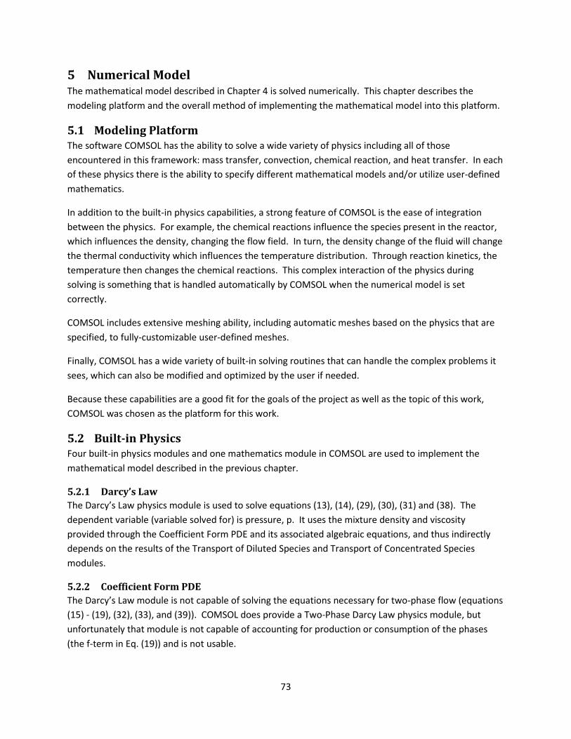
73

5 Numerical Model The mathematical model described in Chapter 4 is solved numerically. This chapter describes the modeling platform and the overall method of implementing the mathematical model into this platform.

5.1 Modeling Platform The software COMSOL has the ability to solve a wide variety of physics including all of those encountered in this framework: mass transfer, convection, chemical reaction, and heat transfer. In each of these physics there is the ability to specify different mathematical models and/or utilize user-defined mathematics.

In addition to the built-in physics capabilities, a strong feature of COMSOL is the ease of integration between the physics. For example, the chemical reactions influence the species present in the reactor, which influences the density, changing the flow field. In turn, the density change of the fluid will change the thermal conductivity which influences the temperature distribution. Through reaction kinetics, the temperature then changes the chemical reactions. This complex interaction of the physics during solving is something that is handled automatically by COMSOL when the numerical model is set correctly.

COMSOL includes extensive meshing ability, including automatic meshes based on the physics that are specified, to fully-customizable user-defined meshes.

Finally, COMSOL has a wide variety of built-in solving routines that can handle the complex problems it sees, which can also be modified and optimized by the user if needed.

Because these capabilities are a good fit for the goals of the project as well as the topic of this work, COMSOL was chosen as the platform for this work.

5.2 Built-in Physics Four built-in physics modules and one mathematics module in COMSOL are used to implement the mathematical model described in the previous chapter.

5.2.1 Darcy’s Law The Darcy’s Law physics module is used to solve equations (13), (14), (29), (30), (31) and (38). The dependent variable (variable solved for) is pressure, p. It uses the mixture density and viscosity provided through the Coefficient Form PDE and its associated algebraic equations, and thus indirectly depends on the results of the Transport of Diluted Species and Transport of Concentrated Species modules.

5.2.2 Coefficient Form PDE The Darcy’s Law module is not capable of solving the equations necessary for two-phase flow (equations (15) - (19), (32), (33), and (39)). COMSOL does provide a Two-Phase Darcy Law physics module, but unfortunately that module is not capable of accounting for production or consumption of the phases (the f-term in Eq. (19)) and is not usable.

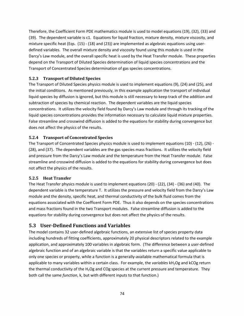
74

Therefore, the Coefficient Form PDE mathematics module is used to model equations (19), (32), (33) and (39). The dependent variable is c1. Equations for liquid fraction, mixture density, mixture viscosity, and mixture specific heat (Eqs. (15) - (18) and (23)) are implemented as algebraic equations using user-defined variables. The overall mixture density and viscosity found using this module is used in the Darcy’s Law module, and the overall specific heat is used by the Heat Transfer module. These properties depend on the Transport of Diluted Species determination of liquid species concentrations and the Transport of Concentrated Species determination of gas species concentrations.

5.2.3 Transport of Diluted Species The Transport of Diluted Species physics module is used to implement equations (9), (24) and (25), and the initial conditions. As mentioned previously, in this example application the transport of individual liquid species by diffusion is ignored, but this module is still necessary to keep track of the addition and subtraction of species by chemical reaction. The dependent variables are the liquid species concentrations. It utilizes the velocity field found by Darcy’s Law module and through its tracking of the liquid species concentrations provides the information necessary to calculate liquid mixture properties. False streamline and crosswind diffusion is added to the equations for stability during convergence but does not affect the physics of the results.

5.2.4 Transport of Concentrated Species The Transport of Concentrated Species physics module is used to implement equations (10) - (12), (26) - (28), and (37). The dependent variables are the gas species mass fractions. It utilizes the velocity field and pressure from the Darcy’s Law module and the temperature from the Heat Transfer module. False streamline and crosswind diffusion is added to the equations for stability during convergence but does not affect the physics of the results.

5.2.5 Heat Transfer The Heat Transfer physics module is used to implement equations (20) - (22), (34) - (36) and (40). The dependent variable is the temperature T. It utilizes the pressure and velocity field from the Darcy’s Law module and the density, specific heat, and thermal conductivity of the bulk fluid comes from the equations associated with the Coefficent Form PDE. Thus it also depends on the species concentrations and mass fractions found in the two Transport modules. False streamline diffusion is added to the equations for stability during convergence but does not affect the physics of the results.

5.3 User-Defined Functions and Variables The model contains 32 user-defined algebraic functions, an extensive list of species property data including hundreds of fitting coefficients, approximately 20 physical descriptors related to the example application, and approximately 100 variables in algebraic form. (The difference between a user-defined algebraic function and of an algebraic variable is that the variables return a specific value applicable to only one species or property, while a function is a generally-available mathematical formula that is applicable to many variables within a certain class. For example, the variables kH2Og and kCOg return the thermal conductivity of the H2Og and COg species at the current pressure and temperature. They both call the same function, k, but with different inputs to that function.)

75

The user-defined functions are listed in Appendix A and variables not already covered in the description of mathematics in Chapter 4 are given in Appendix B.

5.4 Implementing Multi-Physics Integration As mentioned during the description of each physics modules, they are dependent on each other’s dependent variables. COMSOL allows this to be accomplished easily in the setup by specifying as an input to one physics the dependent variable of another. For example, the velocity field in Transport of Diluted Species physics is able to be directly linked to the velocity field solved by the Darcy’s Law physics. This straightforward procedure is followed in all other cases as well.

5.5 Solution Methods The description of Initial Conditions in Section 4.3 touched upon some of the difficulties of running the numerical model, namely the setting of some concentrations initially to values that are not necessarily realistic. In that case, the disadvantage of the non-desired initial values is negated after enough time has progressed to “wash out” the initial species from the reactor.

Another challenge of solving this multi-physics model is the integration of the physics and interdependence of variables. While setting up the model to accomplish this is easy, during solving it is advantageous to solve different physics modules separately in an iterative segregated scheme. In particular, the solver routine solves for the species concentrations and mass fractions (mass transfer) in one step, then for fluid content and pressure (momentum transfer) in another step, then temperature (heat transfer) in a third step. The solver must find a solution that satisfies all three steps simultaneously. While this procedure takes longer to solve than if it solved all dependent variables at the same time, it greatly decreases convergence problems and becomes almost a necessity to solve these complex problems with different physics.

In addition to segregating the variables during solving, it is advantageous to begin the solution from zero time ignoring entirely a dependent variable. This is done for the Heat Transfer physics and temperature. At t=0, the numerical model is run isothermally by disabling the solving of the dependent variable T, instead setting it to a constant. This allows the flows and species to transition from zero-conditions to something closer to steady-state , which may take anywhere from 0.1 to 10 seconds. Once the flows, species, and pressures have been solved to reasonably stable values, then the Heat Transfer physics is enable and T becomes a dependent variable once again, and the simulation proceeds.

The mesh used also plays an important role in the ability to quickly solve the problem numerically and the accuracy of the solution. Because the most difficult convergence happens in the initial stages of solving, using a coarser mesh will speed convergence in this time. However, a too-coarse mesh can cause instabilities within the model that may make it worse. To implement this example application, in the first stage, which is isothermal, a coarser mesh is used, see Figure 19. Then when all physics are solved a finer mesh is used with a gradient focused towards the wall to capture the largest thermal transients, see Figure 20.

76

Figure 19: Coarse mesh (750 elements) used during initial stages of solving. Note that the r-axis is stretched; both r and z axes are units of meters. The axis of symmetry is shown by the red dashed line at r=0.

Figure 20: Finer mesh (2,250 elements) used for solving the complete model. The added resolution in the r-direction is to capture the thermal transient that propagates inward from the exterior wall at r = 0.023 m.

77

6 Simulation Results of Example Application The model framework was applied to the example application discussed at the beginning of Chapter 4, a downflow fixed bed reactor. This chapter describes the particular features of that application and presents the results of the simulation with a comparison to literature. The last section of this chapter discusses how the lessons learned from this simulation could be applied to a reactor for the mobile bio-refinery concept.

6.1 Physical Setup The model framework was applied to the fixed bed reactor geometry shown in Figure 17 and in particular the 2-D axisymmetric representation of a single tube as shown in Figure 18. Jess and Kern [36] simulated the heat and mass transfer (but no prediction of products) of a similar geometry, and so for comparison this framework was applied to that work. The parameters of the reactor are shown in Table 8, and come from the Jess and Kern model unless otherwise noted.

Two simplifying adjustments were made to the model framework in preparation of the results shown here. First, only hydrocarbon species CH4, C6H14, C7H16, and C8H18 were considered as the product in this example. This was done for no other reason than to reduce model complexity and achieve expeditious convergence. Methane was chosen because it is a major hydrocarbon product of FTS. The other three were chosen because they bracket the liquid and gas transition in the product species at the simulated conditions: C6H14 is nearly always a gas, C8H18 is nearly always a liquid, and C7H16 is present as both gas and liquid in the reactor. It is assumed that species with carbon number less than 6 will behave similarly to C6H14 and those with carbon numbers more than 8 will behave similarly to C8H18 with the exception

Table 8: Physical parameters of the example application. Unless noted otherwise, values are taken from Jess and Kern [36].

Parameter Value Comment Reactor height 12 m Reactor interior radius 2.3 cm Superficial gas velocity 0.55 m/s Used as inlet velocity boundary

condition, U0 in Eq. (29). Total pressure 24 bar Used as exit pressure boundary

condition, pexit in Eq. (31). Bulk density of catalyst bed 790 kg/m3 Multiply Eqs. (43) and (47) to

obtain reaction rates in mol/(m3*s)

Inlet concentration of H2 66.6% (vol. basis) Remainder is CO. After conversion, these values are used in Eq. (26).

Cooling water and inlet gas temperatures

240 °C Used in Eqs. (34) and (35).

Bed porosity 0.4 Value of εp in Eqs. (13) and (19) (not from Jess and Kern)

Chain growth probability 0.85 Value of α in Eq. (45) (not from Jess and Kern).

78

being the amount of product produced in each case. Therefore, these four selected product species were deemed sufficient to demonstrate the capabilities of the model framework within the example application. Their relative concentrations were determined in accordance with the theoretical ASF distribution and governed by Eq. (45).

The second adjustment is that binary diffusion coefficients for the gas species were not computed in accordance with Eq. (60) but were rather set to (equal) constants of 10-5 m2/s. Thus no radial mixing will be observed in the results. This effect is expected to be minor and acceptable within the goals of the results and was done for simplicity.

6.2 Results Figure 21 shows the steady-state temperature and pressure contours within the reactor, on the 2-D axisymmetric plane. Note the plane is stretched in the radial direction. Figure 22 shows the same data, but in a 3-D depiction which is the 2-D plane partially rotated about the axis of symmetry. The results show that a hot spot exists approximately 2.5 m from the inlet, at the center of the reactor, and reaches a temperature of 294 °C (567 K). Hot spots near the inlet are expected in this reactor configuration. Pressure decreases consistently from the inlet to the outlet and is uniform in the radial direction as expected.

Figure 21: 2-D axisymmetric view of the pressure and temperature inside the tube at steady-state. A hot spot in the reactor can be seen at approximately r = 0 and z = 9.5 m, or at the center about 2.5 m from the inlet.

79

Figure 22: 3-D view of the pressure and temperature inside the tube at steady -state. The region of the hot spot in the reactor is zoomed in on the left.

Figure 23 shows the results of the Jess and Kern model, where temperature as a function of reactor length (from the inlet) is shown, and the different curves correspond to different cooling water and inlet gas temperatures. For comparison to this work a visual interpolation for a temperature of Tin,cool = 240 °C will have a peak temperature near 2 m from the inlet, with a value between 280° C and 320 °C. This

80

compares well to this work, where Figure 21 (and Figure 22) shows that the maximum temperature is 294 °C and occurs 2.5 m from the reactor inlet. The Jess and Kern result in Figure 24 shows that at Tin,cool

= 240 °C, the maximum temperature expected at the centerline (r=0) is approximately 290 °C, which compares very well to the results of this work.

Figure 23: From the results shown, for T in,cool = 240 °C, it is expected that the hot spot will occur approximately 2 m from the inlet and reach a temperature between 280 °C and 320 °C. Figure 5 from Jess and Kern [36].

Figure 24: From the results shown, the maximum temperature at the centerline for Tin,cool = 240 °C is approximately 290 ° C. Figure 8 from Jess and Kern [36].

81

The results here show a steeper drop in temperature after the hot spot that shown by Jess and Kern. This is likely due to the difference that this model assumes an isothermal temperature of the cooling water (likely resulting in better heat transfer in the hot spot zone) while Jess and Kern take into account the local temperature rise of the cooling water.

Jess and Kern do not attempt to simulate reactions, species concentrations, or other properties throughout the reactor. An advantage to the model in this work is that it can be used to look at these properties and gain additional insight in addition to the heat and mass transfer information. The following figures (Figure 25 through Figure 41) present steady-state results for species concentrations, reaction rates, density, and liquid content for further insight into the operation of the fixed bed reactor under the simulated conditions. For ease of viewing the details, all results are shown in 2-D axisymmetric form. The reader is encouraged to revisit Figure 21 and Figure 22 as needed to note how the 2-D axisymmetric representation relates to the 3-D geometry. The figure captions describe the results, and in general they are all consistent with expectations.

Figure 25: The liquid fraction. The liquid is close to the wall in an annular ring, with the center filled with gas. As pressure decreases down the tube, some liquid changes to gas. Although the temperature profile is relatively constant in the radial direction after the hot-spot at z = 9.5 m, the liquid stays near the outer wall because there is no radial movement of the bulk fluid. The distribution of the primary liquid species C7H16 and C8H18 are shown in Figure 38 and Figure 41, respectively.

82

Figure 26: The density. Density follows liquid fraction (Figure 25) closely, but is more influenced by the decrease in pressure from reactor inlet to outlet.

Figure 27: Rate of the water-gas shift reaction (Eq. (46)). For z < 9.5, the reaction rate is slightly negative in the entire reactor due to the absence of CO, which was consumed at z = 9.5. As soon as more CO is produced, it is consumed by the FT reaction, so the WGS reaction rate remains negative while z < 9.5. When z > 9.5 m, the reaction rate varies in the radial direction, increasing in the direction of decreasing temperature. This correct yet counterintuitive result arises because the WGS reaction indeed behaves this way at conditions encountered: very low water concentrations (cH2O ≅ 0.01) combined with high H2 and CO concentrations.

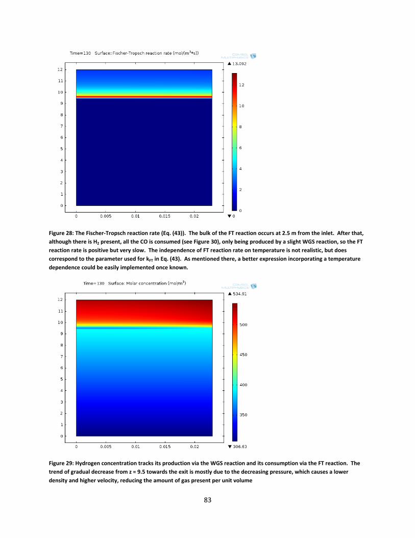
83

Figure 28: The Fischer-Tropsch reaction rate (Eq. (43)). The bulk of the FT reaction occurs at 2.5 m from the inlet. After that, although there is H2 present, all the CO is consumed (see Figure 30), only being produced by a slight WGS reaction, so the FT reaction rate is positive but very slow. The independence of FT reaction rate on temperature is not realistic, but does correspond to the parameter used for kFT in Eq. (43). As mentioned there, a better expression incorporating a temperature dependence could be easily implemented once known.

Figure 29: Hydrogen concentration tracks its production via the WGS reaction and its consumption via the FT reaction. The trend of gradual decrease from z = 9.5 towards the exit is mostly due to the decreasing pressure, which causes a lower density and higher velocity, reducing the amount of gas present per unit volume

84

Figure 30: CO concentration. The effect of the WGS reaction on CO is small (notice no radial variation), so its concentration closely follows that of the FT reaction. By the time the reactants get to z = 9.5 m, all the CO is consumed. Since the WGS reaction is slightly negative for all z < 9.5, CO is being produced in this region but is immediately consumed by the FT reaction, and its concentration remains relatively constant.

Figure 31: CO2 concentration. CO2 is produced via the FT reaction. The slight curvature near the wall is due to the WGS reaction. For z < 9.5, the slightly negative WGS reaction is slowly consuming CO2 which is evident in the gradually decreasing concentration towards the exit.

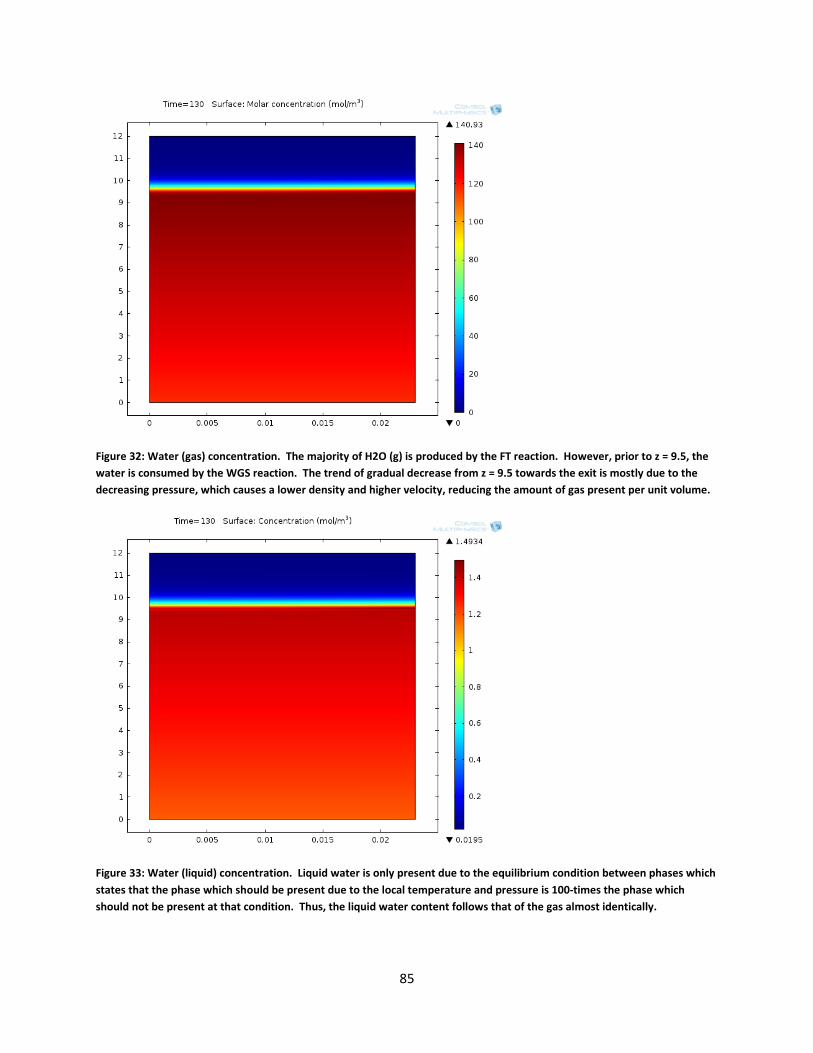
85

Figure 32: Water (gas) concentration. The majority of H2O (g) is produced by the FT reaction. However, prior to z = 9.5, the water is consumed by the WGS reaction. The trend of gradual decrease from z = 9.5 towards the exit is mostly due to the decreasing pressure, which causes a lower density and higher velocity, reducing the amount of gas present per unit volume.

Figure 33: Water (liquid) concentration. Liquid water is only present due to the equilibrium condition between phases which states that the phase which should be present due to the local temperature and pressure is 100-times the phase which should not be present at that condition. Thus, the liquid water content follows that of the gas almost identically.

86

Figure 34: CH4 concentration tracks the FT reaction rate. The trend of gradual decrease from z = 9.5 towards the exit is mostly due to the decreasing pressure, which causes a lower density and higher velocity, reducing the amount of gas present per unit volume.

Figure 35: C6H14 (gas) concentration follows that of the FT reaction rate and the trend is nearly identical to that of CH4, although the amount (moles) of C6H14 produced is much smaller, as expected.

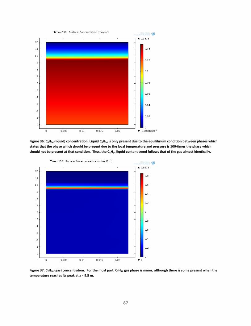
87

Figure 36: C6H14 (liquid) concentration. Liquid C6H14 is only present due to the equilibrium condition between phases which states that the phase which should be present due to the local temperature and pressure is 100-times the phase which should not be present at that condition. Thus, the C6H14 liquid content trend follows that of the gas almost identically.

Figure 37: C7H16 (gas) concentration. For the most part, C7H16 gas phase is minor, although there is some present when the temperature reaches its peak at z = 9.5 m.

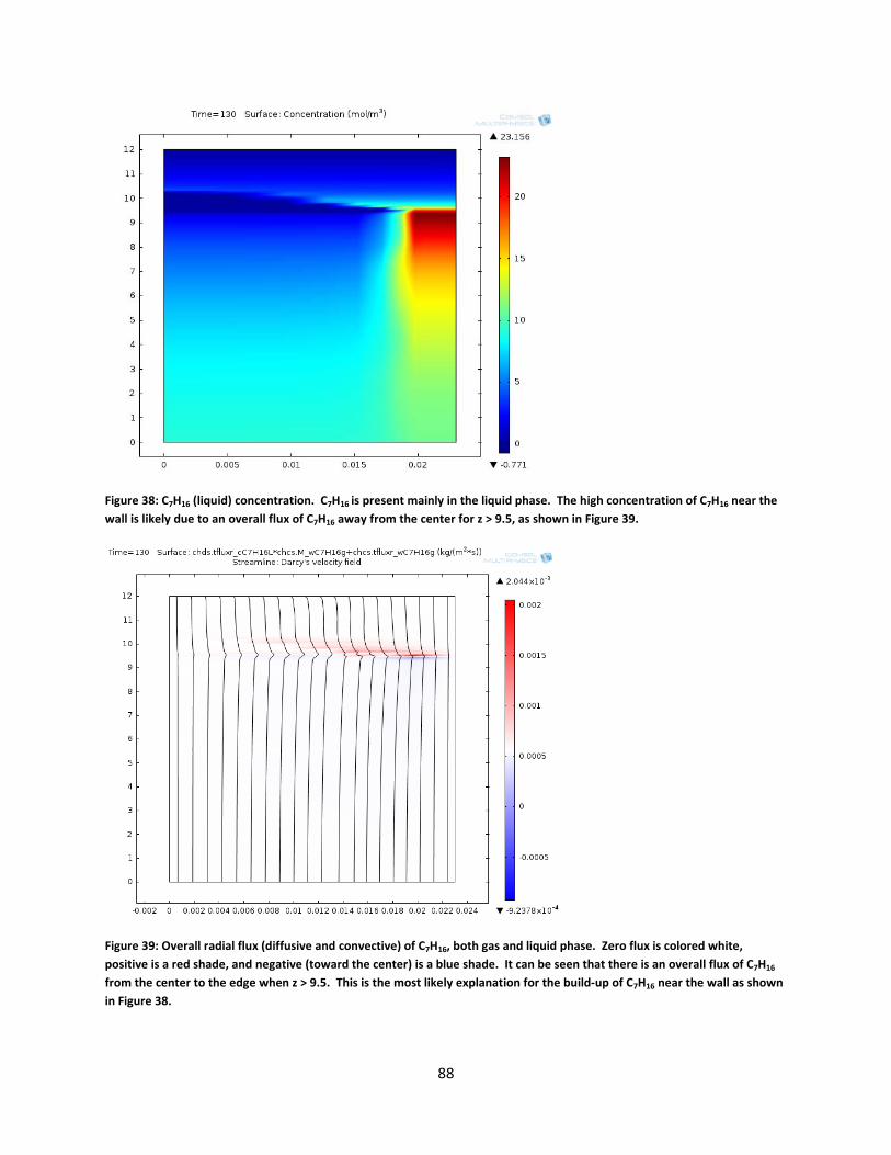
88

Figure 38: C7H16 (liquid) concentration. C7H16 is present mainly in the liquid phase. The high concentration of C7H16 near the wall is likely due to an overall flux of C7H16 away from the center for z > 9.5, as shown in Figure 39.

Figure 39: Overall radial flux (diffusive and convective) of C7H16, both gas and liquid phase. Zero flux is colored white, positive is a red shade, and negative (toward the center) is a blue shade. It can be seen that there is an overall flux of C7H16 from the center to the edge when z > 9.5. This is the most likely explanation for the build-up of C7H16 near the wall as shown in Figure 38.

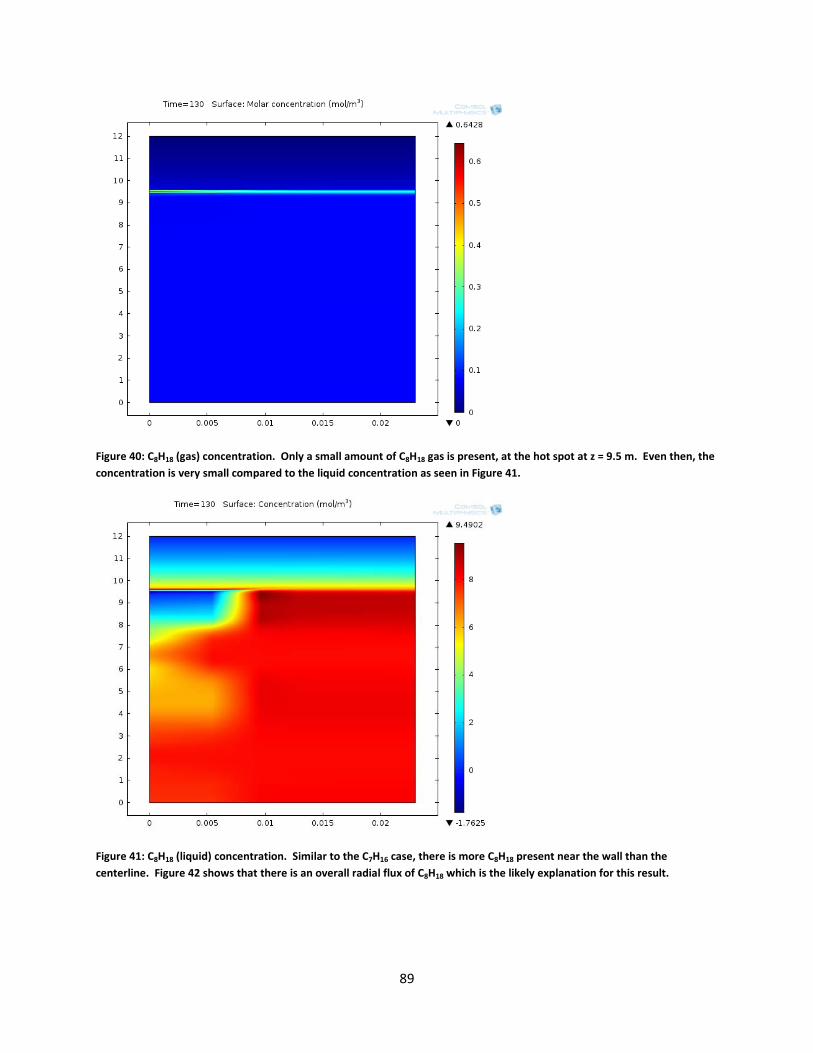
89

Figure 40: C8H18 (gas) concentration. Only a small amount of C8H18 gas is present, at the hot spot at z = 9.5 m. Even then, the concentration is very small compared to the liquid concentration as seen in Figure 41.

Figure 41: C8H18 (liquid) concentration. Similar to the C7H16 case, there is more C8H18 present near the wall than the centerline. Figure 42 shows that there is an overall radial flux of C8H18 which is the likely explanation for this result.

90

Figure 42: Overall radial flux (diffusive and convective) of C8H18, both gas and liquid phase. Zero flux is colored white, positive is a red shade, and negative (toward the center) is a blue shade. It can be seen that there is an overall flux of C8H18 from the center to the edge when z > 9.5, although the effect is not as pronounced as the C7H16 case. This is the most likely explanation for the radial variation in concentration as shown in Figure 41.

6.3 Discussion It is quite clear from the figures that the FT reaction and corresponding production of products is nearly complete within the first 3 m of the reactor length. This is especially evident when looking at CO concentration (Figure 30), which becomes nearly zero after 2.5 m, and the temperature (Figure 21), which has a hot spot corresponding to maximum reaction at about the 2.5 m point. Thus it seems that the rest of the reactor is not participating in the reaction.

In experience with traditional reactors, the location of the hot spot and reaction completion point will progress downwards along the length of the reactor as time of operation increases. This is because the catalyst that is being used the most will gradually become deactivated due to various mechanisms such as poisoning, hydrothermal sintering, degradation, and fouling (with more details described in the literature review, Section 3.2.3.1. The reaction will not occur to the same extent on the deactivated catalyst as before and the reactants will carry further into the reactor bed until they find “fresh” catalyst. Thus the portion of the reactor downstream of the initial reaction completion point is not thought of as “un-used” but rather “in reserve” to extend the life of the reactor between catalyst bed changes.

However, there may be ways to slow down deactivation processes such that the progression of the reaction completion zone down the reactor length becomes much slower. One key to this is proper management of the temperature which not only will reduce thermal and mechanical degradation but also will reduce the potential for hydrothermal sintering if the production (and thus concentration) of

91

water can be more evenly distributed. Therefore, if the heat can be properly managed, there may be an opportunity to reduce the length of the reactor and achieve comparable catalyst bed lifetimes.

Another feature of the reactor that is apparent from the figures is a lack of radial mixing of the species. This can be seen by the distribution of the liquid phase in Figure 25, which shows that the liquid content remains nearly constant at r = 0.0185 m, and also by the fluxes of C7H16 and C8H18 (Figure 39 and Figure 42, respectively) which show that the radial fluxes, while present, are small. This indicates that there is an opportunity to increase the radial mixing with corresponding benefit to evening out the concentrations of reactants and products, and promote better heat exchange.

Another possible way to reduce the hot spot would be to artificially “deactivate” the catalyst near the reactor inlet by diluting it with inert material. With an engineered ratio of inert material to active catalyst that varies with reactor length, the reaction may be made more uniform through the reactor. This ratio as a function of length should also take into account long-term degradation. But in doing so, the overall degradation may be reduced, as discussed above.

Considering these three main lessons learned from the modeling results of the traditional reactor, namely shorter length, greater mixing, and variable active catalyst density, a new reactor concept can be proposed, and is shown in Figure 43. In this reactor, the length is made to 3 m, which is short enough to stand vertically within a standard tractor trailer. Baffles within the reactor promote more radial mixing, and a variable active catalyst density is incorporated to eliminate a hot spot. The feasibility and exact design of this reactor concept could be accomplished with the model framework developed in this work.

Figure 43: Potential FT reactor concept suitable for a mobile bio-refinery.

93

7 Conclusions and Future Work This chapter presents the overall conclusions of this study and recommends potential future work in the area.

7.1 Conclusions The description of Fischer-Tropsch synthesis (FTS) in Chapter 2 showed that it is an attractive option in the process of converting biomass-derived syngas to liquid fuels. The technology is robust and has been practiced for nearly 100 years. In spite of this history, the literature discussed in Chapter 3 shows that the inherent mechanisms by which it works are still not understood. In addition, the majority of experience with FTS is in the context of ever-larger facilities with the basic design of the FTS reactor remaining relatively constant over the years.

In contrast to the current utilization of FTS, it may be advantageous to have the capability of FTS on a much smaller scale, such as mobile bio-refineries that can produce liquid fuel from local resources and easily travel to where the resources are located. An FTS reactor that would be amenable to this type of facility would most likely need to be quite different than the traditional FTS reactors in place now. In particular, the size of the reactor must be reduced such that it would fit on standard tractor-trailer beds.

One way of finding an optimal reactor configuration is the traditional design route of FTS reactors: laboratory test, pilot scale test, and full scale implementation. Alternately, computer simulation can be a more time- and cost-efficient method of achieving the same, if not better, result by looking at a wide variety of physical reactor configurations. Such simulation must be truly predictive and requires understanding and modeling of the core physics that underlie the FTS reactor and cannot rely only the decades of experience that is applicable to only a handful of reactor configurations. Unfortunately, no known comprehensive model has been developed to-date that has this ability.

To address this need, this work examined the four fundamental physics areas that underlie FTS reactors: momentum transport, mass transport, energy transport, and chemical kinetics. In each case it consolidated the research and parts of the theory as applicable to the particular features of an FTS fixed-bed reactor, developing the governing equations, boundary conditions, initial conditions, and constitutive relations for all the physical properties. The successful development of these generalized FTS physics mathematics and their application to an example application (a representative tube within a multi-tubular fixed-bed reactor) is described in this report in Chapter 4.

As a practical matter, the mathematics developed in Chapter 4 were solved numerically. The implementation into the numerical modeling platform COMSOL is described in Chapter 5. A necessary feature of this implementation is the ability for each physics to be dependent on the other. This integration of physics components is one of the inherent capabilities of the COMSOL software. Several methods used to achieve a solution in an expeditious manner are also described in that chapter.

The model developed in this work was applied to a reactor configuration that was simulated by other workers with respect to the heat and mass transfer characteristics. The results compare well for this configuration as illustrated in Chapter 6. It must be emphasized that no features of a fixed-bed FTS

94

reactor were incorporated into the model aside from the geometry and other physical parameters. That is, the general mathematical equations for the underlying physics were not dependent on this application, yet were able to describe the observed phenomena in agreement with the other study.

In addition, the model in the present work was able to predict product species, reaction rates, density, and liquid content for further insight into the processes occurring within the reactor. Through these insights, a new reactor concept incorporating mixing baffles, shorter length, and variable active catalty density was developed that may be suitable for the mobile bio-refinery application.

7.2 Future Work Although the mathematical model as implemented in the COMSOL software was able to predict FTS behavior in the example application, there is still an opportunity to improve it in two general areas: (1) increased accuracy, and (2) faster and more robust solving capability.

To increase the accuracy, it is recommended that the following work be undertaken to improve upon the developed macroscale model. The list has been prioritized based on the expected degree of accuracy improvement that each item would bring.

• Develop and incorporate a temperature-dependency into the FT reaction rate. • Although application-specific, the interface with the cooling water is currently modeled as ideal

and making this more realistic would improve the overall accuracy. • An expected significant enhancement to the macroscale model is expected if the physics can

also be predicted at the microscale, with the results used by the macroscale model. Thus, a companion microscale model should be developed that incorporates the appropriate mathematical relationships to successfully describe the physics surrounding, for example, the kinetics and momentum, mass, and energy transport occurring at and around a single catalyst particle or group of particles. According to the literature, such a model will be a marked improvement above the macroscale models. However, development of such a model and the means of applying it will be an involved undertaking.

• Improve the relations used to simulate phase change kinetics to better-represent reality. • Currently the gas species are modeled as non-ideal only for the determination of enthalpy and

associated heat of reaction. The other physics rely on the ideal gas assumption. Modeling the multicomponent gas mixture as real, including the challenging region near the critical point, for all physics will be an improvement.

• Although the current framework can inherently capture changes with time, such as during startup, changing flowrates or compositions, and cooling water fluctuations, there are no constitutive relations for the changing behavior of the catalyst over time. Degradation effects such as blockage, hydrothermal sintering, and conversion to non-catalytic compounds which occur in actual reactors are currently not able to be captured.

• Incorporate more species, up to C60, with both liquid and gas phases for species C6 – C12, and all associated property data. In addition to the paraffins, include at a minimum olefin species below C20 and possibly alcohols as well.

• Capture deviations from the ideal Anderson-Schulz-Flory distribution of products.

95

• Develop and incorporate a means of predicting the amount of non-paraffin products. • Develop and incorporate a constitutive relation for multicomponent diffusion of liquid species. • Determine and validate the accuracy by (a) more involved comparisons to the models in the

literature, (b) comparisons and simulation of experimental data in the literature, and (c) comparisons to actual reactor data through industrial partners.

To improve the solving capability, the following work is recommended:

• Improve the implementation of phase changes which cause discontinuities in the model. Current smoothing routines may be improved upon to expedite solution finding without compromising accuracy.

• Explore other solving routines such as combinations of iterative and direct solvers, segregating the physics, solving methods that vary with time, etc.

• Perform mesh refinement studies including examination of time-variant meshes.

Incremental improvements to the model framework can be made through work in any of these areas. Thus there exists flexibility in pursuing model improvements that can take into account available resources.

97

References [1] D. H. Petraeus, "Memorandum for the Soldiers, Sailors, Airmen, Marines, and Civilians of US

Forces-Afghanistan," Kabul, Afghanistan, June 7, 2011. [2] B. H. Davis, "Overview of reactors for liquid phase Fischer-Tropsch synthesis," Catalysis Today,

vol. 71, pp. 249-300, 2002. [3] A. de Klerk, Fischer-Tropsch Refining. Germany: Wiley-VCH Verlag & Co., 2011. [4] A. P. Steynberg and M. E. Dry, Eds., Fischer-Tropsch Technology (in Studies in Surface Science

and Catalysis 152, G. Centi, Ed.). Amsterdam: Elsevier B. V., 2004. [5] W. Banholzer, "The Future of Fuels and Alternative Feedstocks: Recognizing Hype vs. Practical

Limitations," presented at the AIChE Annual Meeting, Minneapolis, MN, October 16-21, 2011. [6] (2011) "Report Questions Liklihood of Meeting Biofuels Mandates," Chemical Engineering

Progress, vol. 107, pp. 5-6. [7] A. de Klerk and E. Furimsky, Catalysis in the Refining of Fischer-Tropsch Syncrude. Cambridge,

UK: RSC Publishing, 2010. [8] H. Robota, R. K. Smith, and R. Morris, "The U.S. Air Force's Assured Aerospace Fuels Research

Facility Fischer-Tropsch Liquids Upgrading Reactor," presented at the 2011 AIChE Spring Meeting, Chicago, IL, March 13-17, 2011.

[9] M. Iglesias Gonzalez, B. Kraushaar-Czarnetzki, and G. Schaub, "Process comparison of biomass-to-liquid (BtL) routes Fischer–Tropsch synthesis and methanol to gasoline," Biomass Conversion and Biorefinery, vol. 1, pp. 229-243, 2011.

[10] M. E. Dry, "Fischer-Tropsch synthesis over iron catalysts," Catalysis Letters, vol. 7, pp. 241-251, 1990.

[11] M. E. Dry, "Chemical concepts used for engineering purposes," in Fischer-Tropsch Technology, A. P. Steynberg and M. E. Dry, Eds., ed Amsterdam: Elsevier B. V., 2004, pp. 196-257.

[12] F. Fischer and H. Tropsch, "Process for the Production of Paraffin-Hydrocarbons with More Than One Carbon Atom," United States Patent 1,746,464, 1930.

[13] H. S. Elworthy and E. H. Williamson, "Process of Manufacturing Gas," United States Patent 738,303, 1903.

[14] A. Mittasch and C. Schneider, "Producing Compounds Containing Carbon and Hydrogen," United States Patent 1,201,850, 1916.

[15] A. E. Miller, "The Story of the Technical Oil Mission," presented at the Twenty-fifth Annual Meeting of the American Petroleum Institute, Chicago, IL, November 14, 1945.

[16] P. W. Cornell and E. Cotton, "Catalytic Reactor," United States Patent 2,585,441, 1952. [17] H. C. Henry and J. B. Gilbert, "Scale Up of Pilot Plant Data for Catalytic Hydroprocessing,"

Industrial & Engineering Chemistry Process Design and Development, vol. 12, pp. 328-334, 1973. [18] R. Guettel and T. Turek, "Comparison of different reactor types for low temperature Fischer-

Tropsch synthesis: A simulation study," Chemical Engineering Science, vol. 64, pp. 955-964, 2009.

[19] R. J. Madon and W. F. Taylor, "Fischer-Tropsch synthesis on a precipitated iron catalyst," Journal of Catalysis, vol. 69, pp. 32-43, 1981.

[20] A. de Klerk, "Liquid holdup in packed beds at low mass flux," AIChE Journal, vol. 49, pp. 1597-1600, 2003.

[21] A. P. Steynberg, "Introduction to Fischer-Tropsch Technology," in Fischer-Tropsch Technology, A. P. Steynberg and M. E. Dry, Eds., ed Amsterdam: Elsevier B. V., 2004, pp. 1-63.

[22] A. P. Steynberg, M. E. Dry, B. H. Davis, and B. B. Breman, "Fischer-Tropsch Reactors," in Fischer-Tropsch Technology, A. P. Steynberg and M. E. Dry, Eds., ed Amsterdam: Elsevier B. V., 2004, pp. 64-195.

98

[23] L. Guillou, S. Paul, and V. Le Courtois, "Investigation of H2 staging effects on CO conversion and product distribution for Fischer-Tropsch synthesis in a structured microchannel reactor," Chemical Engineering Journal, vol. 136, pp. 66-76, 2008.

[24] A. K. Saroha and R. Khera, "Hydrodynamic study of fixed beds with cocurrent upflow and downflow," Chemical Engineering and Processing, vol. 45, pp. 455-460, 2006.

[25] M. F. M. Post, A. C. Van't Hoog, J. K. Minderhoud, and S. T. Sie, "Diffusion limitations in fischer-tropsch catalysts," AIChE Journal, vol. 35, pp. 1107-1114, 1989.

[26] J. W. Niemantsverdriet, A. M. Van der Kraan, W. L. Van Dijk, and H. S. Van der Baan, "Behavior of metallic iron catalysts during Fischer-Tropsch synthesis studied with Moessbauer spectroscopy, x-ray diffraction, carbon content determination, and reaction kinetic measurements," The Journal of Physical Chemistry, vol. 84, pp. 3363-3370, 1980.

[27] D. B. Bukur, X. Lang, D. Mukesh, W. H. Zimmerman, M. P. Rosynek, and C. Li, "Binder/support effects on the activity and selectivity of iron catalysts in the Fischer-Tropsch synthesis," Industrial & Engineering Chemistry Research, vol. 29, pp. 1588-1599, 1990.

[28] M. E. Dry, "The Fischer-Tropsch process - commercial aspects," Catalysis Today, vol. 6, pp. 183-206, 1990.

[29] H. Schulz, E. ven Steen, and M. Claeys, "Selectivity and mechanism of Fischer-Tropsch synthesis with iron and cobalt catalysts," in Natural Gas Conversion II - Proceedings of the Third Natural Gas Conversion Symposium, H. E. Curry-Hyde and R. F. Howe, Eds., ed: Elsevier, 1994, pp. 455-460.

[30] M. H. Al-Dahhan and M. P. Dudukovic, "Catalyst wetting efficiency in trickle-bed reactors at high pressure," Chemical Engineering Science, vol. 50, pp. 2377-2389, 1995.

[31] M. R. Khadilkar, Y. X. Wu, M. H. Al-Dahhan, M. P. Dudukovic, and M. Colakyan, "Comparison of trickle-bed and upflow reactor performance at high pressure: Model predictions and experimental observations," Chemical Engineering Science, vol. 51, pp. 2139-2148, 1996.

[32] K. P. de Jong, M. F. M. Post, and A. Knoester, "Deposition of iron from iron-carbonyl onto a working Co-based Fischer Tropsch catalyst: The serendipitious discovery of a direct probe for diffusion limitation," in Natural Gas Conversion V, Proceedings of the 5th International Natural Gas Conversion Symposium, A. Parmaliana, D. Sanfilippo, F. Frusteri, A. Vaccari, and F. Arena, Eds., ed: Elsevier, 1998, pp. 119-124.

[33] S. T. Sie and R. Krishna, "Fundamentals and selection of advanced Fischer-Tropsch reactors," Applied Catalysis A: General, vol. 186, pp. 55-70, 1999.

[34] E. Iglesia, "Design, synthesis, and use of cobalt-based Fischer-Tropsch synthesis catalysts," Applied Catalysis A: General, vol. 161, pp. 59-78, 1997.

[35] G. F. Froment and K. B. Bischoff, Chemical Reactor Analysis and Design. New York: John Wiley & Sons, 1979.

[36] A. Jess and C. Kern, "Modeling of Multi-Tubular Reactors for Fischer-Tropsch Synthesis," Chemical Engineering & Technology, vol. 32, pp. 1164-1175, 2009.

[37] G. P. van der Laan, "Kinetics, Selectivity and Scale Up of the Fischer-Tropsch Synthesis," Ph.D. Thesis, University of Groningen, Groningen, Netherlands, 1999.

[38] P. J. van Berge, "Fischer-Tropsch Studies in the Slurry Phase Favouring Wax Production," Ph.D. Thesis, Department of Chemical Engineering, North-West University (formerly Potchefstroom University for Christian Higher Education (Potchefstroomse Universiteit vir Christelike Hoer Onderwys)), Potchefstroom, South Africa, 1994.

[39] L. P. Zhou, X. Hao, J. H. Gao, Y. Yang, B. S. Wu, J. A. Xu, Y. Y. Xu, and Y. W. Li, "Studies and Discriminations of the Kinetic Models for the Iron-Based Fischer-Tropsch Catalytic Reaction in a Recycle Slurry Reactor," Energy & Fuels, vol. 25, pp. 52-59, Jan 2011.

99

[40] E. S. Lox and G. F. Froment, "Kinetics of the Fischer-Tropsch reaction on a precipitated promoted iron catalyst. 1. Experimental procedure and results," Industrial & Engineering Chemistry Research, vol. 32, pp. 61-70, 1993.

[41] Y.-N. Wang, W.-P. Ma, Y.-J. Lu, J. Yang, Y.-Y. Xu, H.-W. Xiang, Y.-W. Li, Y.-L. Zhao, and B.-J. Zhang, "Kinetics modelling of Fischer-Tropsch synthesis over an industrial Fe-Cu-K catalyst," Fuel, vol. 82, pp. 195-213, 2003.

[42] R. L. Zhang, J. Chang, Y. Y. Xu, L. R. Cao, Y. W. Li, and J. L. Zhou, "Kinetic Model of Product Distribution over Fe Catalyst for Fischer-Tropsch Synthesis," Energy & Fuels, vol. 23, pp. 4740-4747, Oct 2009.

[43] Y.-N. Wang, Y.-Y. Xu, Y.-W. Li, Y.-L. Zhao, and B.-J. Zhang, "Heterogeneous modeling for fixed-bed Fischer-Tropsch synthesis: Reactor model and its applications," Chemical Engineering Science, vol. 58, pp. 867-875, 2003.

[44] E. Iglesia, S. C. Reyes, R. J. Madon, and S. L. Soled, "Selectivity Control and Catalyst Design in the Fischer-Tropsch Synthesis: Sites, Pellets, and Reactors," in Advances in Catalysis. vol. Volume 39, H. P. D.D. Eley and B. W. Paul, Eds., ed: Academic Press, 1993, pp. 221-302.

[45] F. G. Botes and B. B. Breman, "Development and Testing of a New Macro Kinetic Expression for the Iron-Based Low-Temperature Fischer−Tropsch Reaction," Industrial & Engineering Chemistry Research, vol. 45, pp. 7415-7426, 2006.

[46] F. G. Botes, "The Effects of Water and CO2 on the Reaction Kinetics in the Iron-Based Low-Temperature Fischer-Tropsch Synthesis: A Literature Review," Catalysis Reviews-Science and Engineering, vol. 50, pp. 471-491, 2008.

[47] F. G. Botes, "Proposal of a New Product Characterization Model for the Iron-Based Low-Temperature Fischer−Tropsch Synthesis," Energy & Fuels, vol. 21, pp. 1379-1389, 2007.

[48] P. Chaumette, C. Verdon, and P. Boucot, "Influence of the hydrocarbons distribution on the heat produced during Fischer-Tropsch synthesis," Topics in Catalysis, vol. 2, pp. 301-311, 1995.

[49] G. P. van der Laan and A. A. C. M. Beenackers, "Hydrocarbon Selectivity Model for the Gas−Solid Fischer−Tropsch Synthesis on Precipitated Iron Catalysts," Industrial & Engineering Chemistry Research, vol. 38, pp. 1277-1290, 1999.

[50] H. Schulz and M. Claeys, "Kinetic modelling of Fischer-Tropsch product distributions," Applied Catalysis A: General, vol. 186, pp. 91-107, 1999.

[51] M. E. Dry, "Advances in Fishcher-Tropsch Chemistry," Product R&D, vol. 15, pp. 282-286, 1976. [52] M. E. Dry, "FT Catalysts," in Fischer-Tropsch Technology, A. P. Steynberg and M. E. Dry, Eds., ed

Amsterdam: Elsevier B. V., 2004, pp. 533-600. [53] Y. H. Kim, D. Y. Hwang, S. H. Song, S. B. Lee, E. D. Park, and M. J. Park, "Kinetic parameter

estimation of the Fischer-Tropsch synthesis reaction on K/Fe-Cu-Al catalysts," Korean Journal of Chemical Engineering, vol. 26, pp. 1591-1600, Nov 2009.

[54] E. S. Lox and G. F. Froment, "Kinetics of the Fischer-Tropsch reaction on a precipitated promoted iron catalyst. 2. Kinetic modeling," Industrial & Engineering Chemistry Research, vol. 32, pp. 71-82, 1993.

[55] M. Ojeda, R. Nabar, A. U. Nilekar, A. Ishikawa, M. Mavrikakis, and E. Iglesia, "CO activation pathways and the mechanism of Fischer-Tropsch synthesis," Journal of Catalysis, vol. 272, pp. 287-297, Jun 2010.

[56] L. Tian, C.-F. Huo, D.-B. Cao, Y. Yang, J. Xu, B.-S. Wu, H.-W. Xiang, Y.-Y. Xu, and Y.-W. Li, "Effects of reaction conditions on iron-catalyzed Fischer-Tropsch synthesis: A kinetic Monte Carlo study," Journal of Molecular Structure: THEOCHEM, vol. 941, pp. 30-35, 2010.

[57] J. M. Bucher, "The Effect of Interference Techniques on Fischer-Tropsch Product Distributions," Ph.D., Chemical Engineering, University of Michigan, Ann Arbor, MI, 2010.

100

[58] M. Ojeda, A. Li, R. Nabar, A. U. Nilekar, M. Mavrikakis, and E. Iglesia, "Kinetically Relevant Steps and H2/D2 Isotope Effects in Fischer−Tropsch Synthesis on Fe and Co Catalysts," The Journal of Physical Chemistry C, vol. 114, pp. 19761-19770, 2010.

[59] B. W. Wojciechowski, "The Kinetics of the Fischer-Tropsch Synthesis," Catalysis Reviews, vol. 30, pp. 629-702, 1988/12/01 1988.

[60] J. Cheng, P. Hu, P. Ellis, S. French, G. Kelly, and C. Lok, "Some Understanding of Fischer–Tropsch Synthesis from Density Functional Theory Calculations," Topics in Catalysis, vol. 53, pp. 326-337, 2010.

[61] M. R. Rahimpour, A. Mirvakili, and K. Paymooni, "A novel water perm-selective membrane dual-type reactor concept for Fischer-Tropsch synthesis of GTL (gas to liquid) technology," Energy, vol. 36, pp. 1223-1235, 2011.

[62] J. A. Moulijn, A. E. van Diepen, and F. Kapteijn, "Catalyst deactivation: is it predictable?: What to do?," Applied Catalysis A: General, vol. 212, pp. 3-16, 2001.

[63] C. H. Bartholomew, "Mechanisms of catalyst deactivation," Applied Catalysis A: General, vol. 212, pp. 17-60, 2001.

[64] G. F. Froment, "Modeling of catalyst deactivation," Applied Catalysis A: General, vol. 212, pp. 117-128, 2001.

[65] R. Philippe, M. Lacroix, L. Dreibine, C. Pham-Huu, D. Edouard, S. Savin, F. Luck, and D. Schweich, "Effect of structure and thermal properties of a Fischer-Tropsch catalyst in a fixed bed," Catalysis Today, vol. 147, pp. S305-S312, 2009.

[66] M. C. Cassanello, O. M. Martinez, and A. L. Cukierman, "Effect of the liquid axial dispersion on the behavior of fixed bed three phase reactors," Chemical Engineering Science, vol. 47, pp. 3331-3338, 1992.

[67] I. Derevich, V. Ermolaev, and V. Mordkovich, "Liquid-vapor thermodynamic equilibrium in Fischer-Tropsch synthesis products," Theoretical Foundations of Chemical Engineering, vol. 42, pp. 216-219, 2008.

[68] C. L. Yaws. (2003, Aug 23, 2011). Yaws' Handbook of Thermodynamic and Physical Properties of Chemical Compounds. Available: http://www.knovel.com/web/portal/browse/display?_EXT_KNOVEL_DISPLAY_bookid=667

[69] C. L. Yaws, "Thermal Conductivity of Gas - Organic Compounds," in Transport Properties of Chemicals and Hydrocarbons, C. L. Yaws, Ed., ed Boston: William Andrew Publishing, 2009, pp. 201-291.

[70] C. L. Yaws, "Thermal Conductivity of Gas - Inorganic Compounds," in Transport Properties of Chemicals and Hydrocarbons, C. L. Yaws, Ed., ed Boston: William Andrew Publishing, 2009, pp. 292-298.

[71] C. L. Yaws, "Thermal Conductivity of Liquid - Organic Compounds," in Transport Properties of Chemicals and Hydrocarbons, C. L. Yaws, Ed., ed Boston: William Andrew Publishing, 2009, pp. 299-395.

[72] C. L. Yaws, "Thermal Conductivity of Liquid - Inorganic Compounds," in Transport Properties of Chemicals and Hydrocarbons, C. L. Yaws, Ed., ed Boston: William Andrew Publishing, 2009, pp. 396-402.

[73] C. L. Yaws, "Thermal Conductivity of Solid - Inorganic Compounds," in Transport Properties of Chemicals and Hydrocarbons, C. L. Yaws, Ed., ed Boston: William Andrew Publishing, 2009, pp. 403-406.

[74] C. L. Yaws and P. Bahadur, "Viscosity of Gas - Organic Compounds," in Transport Properties of Chemicals and Hydrocarbons, C. L. Yaws, Ed., ed Boston: William Andrew Publishing, 2009, pp. 1-92.

http://www.knovel.com/web/portal/browse/display?_EXT_KNOVEL_DISPLAY_bookid=667

101

[75] C. L. Yaws and J. A. Gomes, "Viscosity of Gas - Inorganic Compounds," in Transport Properties of Chemicals and Hydrocarbons, C. L. Yaws, Ed., ed Boston: William Andrew Publishing, 2009, pp. 93-100.

[76] C. L. Yaws and J. A. Gomes, "Viscosity of Liquid - Inorganic Compounds," in Transport Properties of Chemicals and Hydrocarbons, C. L. Yaws, Ed., ed Boston: William Andrew Publishing, 2009, pp. 194-200.

[77] C. L. Yaws and L. Le Xuan Dang, "Viscosity of Liquid - Organic Compounds," in Transport Properties of Chemicals and Hydrocarbons, C. L. Yaws, Ed., ed Boston: William Andrew Publishing, 2009, pp. 101-193.

[78] C. L. Yaws and P. K. Narasimhan, "Critical properties and acentric factor--Organic compounds," in Thermophysical Properties of Chemicals and Hydrocarbons, C. L. Yaws, Ed., ed Norwich, NY: William Andrew Publishing, 2009, pp. 1-95.

[79] C. L. Yaws and P. K. Narasimhan, "Chapter 19 - Dipole moment—Organic compounds," in Thermophysical Properties of Chemicals and Hydrocarbons, C. L. Yaws, Ed., ed Norwich, NY: William Andrew Publishing, 2009, pp. 672-682.

[80] C. L. Yaws and R. W. Pike, "Chapter 3 - Density of liquid—Organic compounds," in Thermophysical Properties of Chemicals and Hydrocarbons, C. L. Yaws, Ed., ed Norwich, NY: William Andrew Publishing, 2009, pp. 106-197.

[81] C. L. Yaws and P. C. Richmond, "Appendix B - Thermophysical and Transport Properties of Water," in Thermophysical Properties of Chemicals and Hydrocarbons, C. L. Yaws, Ed., ed Norwich, NY: William Andrew Publishing, 2009, pp. 791-799.

[82] C. L. Yaws and M. A. Satyro, "Chapter 20 - Dipole moment—Inorganic compounds," in Thermophysical Properties of Chemicals and Hydrocarbons, C. L. Yaws, Ed., ed Norwich, NY: William Andrew Publishing, 2009, pp. 683-685.

[83] C.-Y. Wang and C. Beckermann, "A two-phase mixture model of liquid-gas flow and heat transfer in capillary porous media—I. Formulation," International Journal of Heat and Mass Transfer, vol. 36, pp. 2747-2758, 1993.

[84] F. G. Botes, "Kinetic and Selectivity Modelling of the Iron-Based Low-Temperature Fischer-Tropsch Synthesis," Ph.D. Thesis, Eindhoven University of Technology (Technische Universiteit Eindhoven), Eindhoven, Netherlands, 2008.

[85] R. R. Davda, J. W. Shabaker, G. W. Huber, R. D. Cortright, and J. A. Dumesic, "A review of catalytic issues and process conditions for renewable hydrogen and alkanes by aqueous-phase reforming of oxygenated hydrocarbons over supported metal catalysts," Applied Catalysis B: Environmental, vol. 56, pp. 171-186, 2005.

[86] A. Burcat and B. Ruscic, "Third Millennium Ideal Gas and Condensed Phase Thermochemical Database for Combustion with Updates from Active Thermochemical Tables," Argonne National Laboratory, Report ANL-05/20 TAE 960, 2005.

[87] S. M. Walas, Phase Equilibria in Chemical Engineering. Stoneham, MA: Butterworth Publishers, 1985.

[88] R. Taylor and R. Krishna, Multicomponent Mass Transfer. New York: John Wiley & Sons, 1993. [89] E. L. Cussler, Diffusion: Mass Transfer in Fluid Systems. New York: Cambridge University Press,

2009. [90] B. E. Poling, J. M. Prausnitz, and J. P. O'Connell, The Properties of Gases and Liquids, 5th Edition.

New York: McGraw-Hill, 2001.

102

Appendix A: User Defined Functions The table below lists the user-defined functions in the COMSOL model.

Function Name

Description Units Expression Arguments

MW Molecular weight g/mol 12.011*numC+2.016/2*numH+31.999/2*numO +28.013/2*numN

numC, numH, numO, numN

rho_gas Density of an individual (ideal) gas species

kg/m3 MW*p/(R_const*T) MW, p, T

rho_liq Density of an individual liquid species (Yaws correlation)

kg/m3 1000*Arho*Brho^(-(1-T/Crho)^nrho) T, Arho, Brho, Crho, nrho

visc_gas Viscosity of an individual gas species (Yaws correlation)

Pa*s (Avisc+Bvisc*T+Cvisc*T^2+Dvisc*T^3)/10E7 T, Avisc, Bvisc, Cvisc, Dvisc

visc_liq Viscosity of an individual liquid species (Yaws correlation)

Pa*s (10^(Avisc+Bvisc/T+Cvisc*T+Dvisc*(T^2)))/10E3 T, Avisc, Bvisc, Cvisc, Dvisc

Vb Normal volume at the boiling point

m^3/mol MW/rho_liq(Tboil, Arho, Brho, Crho, nrho) MW, Tboil, Arho, Brho, Crho, nrho

D_liq Liquid diffusivity m2/s 5.88E-17*T*sqrt(phi_diff*MW_solvent) /(eta_solvent*Vb_solute^0.6)

T, MW_solvent, eta_solvent, Vb_solute

Cp Specific heat (Yaws correlation)

J/(mol*K) Al+Bl*T+Cl*T^2+Dl*T^3 T, Al, Bl, Cl, Dl

h Enthalpy (Yaws correlation)

kJ/mol hfgas298-hvap298+(Al*(T-298.15)+Bl/2*(T^2-298.15^2) +Cl/3*(T^3-298.15^3)+Dl/4*(T^4-298.15^4))/1000

T, hfgas298, hvap298, Al, Bl, Cl, Dl

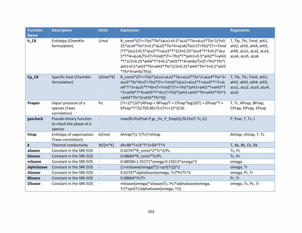
103

Function Name


h_CK Enthalpy (ChemKin formulation)

J/mol R_const*((T<=Tlo)*Tlo*(aLo1+0.5*aLo2*Tlo+aLo3*Tlo^2/3+0.25*aLo4*Tlo^3+0.2*aLo5*Tlo^4+aLo6/Tlo)+(T>Tlo)*(T<=Tmid)*T*(aLo1+0.5*aLo2*T+aLo3*T^2/3+0.25*aLo4*T^3+0.2*aLo5*T^4+aLo6/T)+(T>Tmid)*(T<=Thi)*T*(aHi1+0.5*aHi2*T+aHi3*T^2/3+0.25*aHi4*T^3+0.2*aHi5*T^4+aHi6/T)+(T>Thi)*Thi*(aHi1+0.5*aHi2*Thi+aHi3*Thi^2/3+0.25*aHi4*Thi^3+0.2*aHi5*Thi^4+aHi6/Thi))

T, Tlo, Thi, Tmid, aHi1, aHi2, aHi3, aHi4, aHi5, aHi6, aLo1, aLo2, aLo3, aLo4, aLo5, aLo6

Cp_CK Specific heat (ChemKin formulation)

J/(mol*K) R_const*((T<=Tlo)*(aLo1+aLo2*Tlo+aLo3*Tlo^2+aLo4*Tlo^3+aLo5*Tlo^4)+(T>Tlo)*(T<=Tmid)*(aLo1+aLo2*T+aLo3*T^2+aLo4*T^3+aLo5*T^4)+(T>Tmid)*(T<=Thi)*(aHi1+aHi2*T+aHi3*T^2+aHi4*T^3+aHi5*T^4)+(T>Thi)*(aHi1+aHi2*Thi+aHi3*Thi^2+aHi4*Thi^3+aHi5*Thi^4))

T, Tlo, Thi, Tmid, aHi1, aHi2, aHi3, aHi4, aHi5, aLo1, aLo2, aLo3, aLo4, aLo5

Pvapor Vapor pressure of a species (Yaws correlation)

Pa (Tr<1)*(10^(APvap + BPvap/T + CPvap*log10(T) + DPvap*T + EPvap*T^2)/750.0617)+(Tr>=1)*1E10

T, Tr, APvap, BPvap, CPvap, DPvap, EPvap

gascheck Pseudo-binary function to check the phase of a species

- max(flc1hs(Psat-P,gc_Hv_P_Step(t)),flc1hs(T-Tc,1)) P, Psat, T, Tc, t

hVap Enthalpy of vaporization (Yaws correlation)

kJ/mol AhVap*(1-T/Tc)^nhVap AhVap, nhVap, T, Tc

k Thermal conductivity W/(m*K) Ak+Bk*T+Ck*T^2+Dk*T^3 T, Ak, Bk, Ck, Dk aSoave Constant in the SRK EOS - 0.42747*R_const^2*Tc^2/Pc Tc, Pc bSoave Constant in the SRK EOS - 0.08664*R_const*Tc/Pc Tc, Pc mSoave Constant in the SRK EOS - 0.48508+1.55171*omega-0.15613*omega^2 omega alphaSoave Constant in the SRK EOS - (1+mSoave(omega)*(1-sqrt(Tr)))^2 omega, Tr ASoave Constant in the SRK EOS - 0.42747*alphaSoave(omega, Tr)*Pr/Tr^2 omega, Pr, Tr BSoave Constant in the SRK EOS - 0.08664*Pr/Tr Pr, Tr DSoave Constant in the SRK EOS - mSoave(omega)*aSoave(Tc, Pc)*alphaSoave(omega,

Tr)*sqrt(Tr/alphaSoave(omega, Tr)) omega, Tc, Pc, Tr

104

Function Name


b_z Constant used in algebraically solving the SRK EOS

- ASoave(omega, Pr, Tr)-BSoave(Pr, Tr)-BSoave(Pr, Tr)^2 omega, Pr, Tr

c_z Constant used in algebraically solving the SRK EOS

- -ASoave(omega, Pr, Tr)*BSoave(Pr, Tr) omega, Pr, Tr

Q_z Constant used in algebraically solving the SRK EOS

- ((-1)^2-3*b_z(omega, Pr, Tr))/9 omega, Pr, Tr

R_z Constant used in algebraically solving the SRK EOS

- (2*(-1)^3 - 9*(-1)*b_z(omega, Pr, Tr) +27*c_z(omega,Pr,Tr))/54

omega, Pr, Tr

M_z Constant used in algebraically solving the SRK EOS

- R_z(omega, Pr, Tr)^2 - Q_z(omega, Pr, Tr)^3 omega, Pr, Tr

phi_z Constant used in algebraically solving the SRK EOS

- acos(R_z(omega, Pr, Tr)/sqrt(Q_z(omega, Pr, Tr)^3)) omega, Pr, Tr

S_z Constant used in algebraically solving the SRK EOS

- (-sign(R_z(omega, Pr, Tr))^3)*((abs(R_z(omega, Pr, Tr)) +sqrt(M_z(omega, Pr, Tr)))^(1/3))

omega, Pr, Tr

T_z Constant used in algebraically solving the SRK EOS

- Q_z(omega, Pr, Tr)/S_z(omega, Pr, Tr) omega, Pr, Tr

Z_z Compressibility factor resulting from the SRK -EOS

- gascheck*(max(max(r1z,r2z),r3z)) +liqcheck*(min(min(r1z,r2z),r3z))

gascheck, liqcheck, r1z, r2z, r3z

105

Function Name


h_residual Difference between ideal gas enthalpy and real enthalpy as calculated by the SRK EOS

J/mol R_const*T*(1-Z_z+ASoave(omega, Pr, Tr)/BSoave(Pr, Tr) *(1+DSoave(omega, Tc, Pc, Tr)/(aSoave(Tc, Pc) *alphaSoave(omega, Tr)))*log(1+BSoave(Pr, Tr)/Z_z))

T, omega, Pr, Tr, Tc, Pc, Z_z

106

Appendix B: Selected Variables The table below lists user-defined functions in the COMSOL model not already described in the Mathematical Model chapter.

Variable Description Units Expression H_i Enthalpy of reaction I

(not phase change) J/mol sum(h_products)-sum(h_reactants)

Q_i Heat of reaction i W/m3 -r_i*H_i r_i(phase change)

Reaction rate for a phase-change reaction

mol/(m3*s)

kr_phase*((gascheck_i*Keq_phase+liqcheck_i/Keq_phase)*c_iL-chcs.c_w_ig)

H_i(phase change)

Enthalpy of reaction (phase change)

J/mol if(Tr_i<1,hVap(AhVap_i,nhVap_i,T_eq[1/K],Tc_i[1/K]),0)

gascheck_i Pseudo-binary variable to check the phase of a species

- gascheck(p_eq[1/Pa],Pvap_H2O[1/Pa],T_eq[1/K],Tc_H2O[1/K],t[1/s])

liqcheck_i Pseudo-binary variable to check the phase of a species

- 1-gascheck_i

Tr_i Reduced temperature - T/Tc_i Pr_i Reduced pressure - P/Pc_i r1_i First root of SRK EOS - if(M_z(omegaSoave_i,Pr_i,Tr_i)<0,

(-(2*sqrt(Q_z(omegaSoave_i,Pr_i,Tr_i)) *cos(phi_z(omegaSoave_i,Pr_i,Tr_i)/3))- (-1)/3), (S_z(omegaSoave_i,Pr_i,Tr_i)+ T_z(omegaSoave_i,Pr_i,Tr_i) -(-1)/3))

r2_i Second root of SRK EOS - if(M_z(omegaSoave_i,Pr_i,Tr_i)<0, (-(2*sqrt(Q_z(omegaSoave_i,Pr_i,Tr_i)) *cos((phi_z(omegaSoave_i,Pr_i,Tr_i)+2*pi)/3)) -(-1)/3),r1_i)

r3_i Third root of SRK EOS - if(M_z(omegaSoave_i,Pr_i,Tr_i)<0, (-(2*sqrt(Q_z(omegaSoave_i,Pr_i,Tr_i)) *cos((phi_z(omegaSoave_i,Pr_i,Tr_i)-2*pi)/3)) -(-1)/3),r1_i)

107

Variable Description Units Expression z_i Resulting compressibility

factor for a species based on the SRK EOS at the local temperature and pressure.

- Z_z(gascheck_i,liqcheck_i,r1_i,r2_i,r3_i)

108

Distribution 1 MS0359 LDRD Office c/o Donna L. Chavez 01911 1 MS9051 Imane Khalil 08366 (electronic copy) 1 MS9051 Joseph W. Pratt 08366 1 MS9052 Daniel Dedrick 08367 (electronic copy) 1 MS9052 Chris Shaddix 08367 1 MS9054 Bob Carling 08300 (electronic copy) 1 MS9054 Art Pontau 08360 (electronic copy) 1 MS9291 Blake Simmons 08630 (electronic copy) 1 MS0899 Technical Library 09536 (electronic copy) 1 MS9018 Central Technical Files 08944

a fischer-tropsch synthesis reactor model framework for ... · a fischer-tropsch synthesis reactor...

Documents