a guide to scatterplot and biplot calibration - the … · · 2015-02-19a guide to scatterplot...

A Guide to Scatterplot and Biplot Calibration

version 1.7.2

Jan Graffelman

Department of Statistics and Operations ResearchUniversitat Politecnica de Catalunya

Avinguda Diagonal 647, 08028 Barcelona, Spain.email: [email protected]

September 2012

1 Introduction

This guide gives detailed instructions on how to calibrate axes in scatterplots andbiplots obtained in the statistical environment R [R Development Core Team (2004)]by using the package calibrate. By calibration we refer to the procedure ofdrawing a (linear) scale along an axis in a plot with tick marks and numericlabels. In an ordinary scatter plot of two variables x and y two calibratedperpendicular scales are typically automatically produced by the routine usedfor plotting the two variables. However, scatter plots can be extended withadditional variables that are represented on oblique additional axes. The soft-ware described in this guide can be used to create calibrated scales on theseoblique additional axes. Moreover, in a multivariate setting with more thantwo variables, raw data matrices, correlation matrices, contingency tables, re-gression coefficients, etc. are often represented graphically by means of bi-plots [Gabriel, 1971]. Biplots also contain oblique axes representing variables.The described software can also be used to construct scales on biplot axes.

The outline of this guide is as follows. In Section 2 we indicate how the Rpackage calibrate can be installed. Section 3 describes in detail how to cali-brate additional axes in scatter plots. Section 4 treats the calibration of biplotaxes. Several subsections follow with detailed instructions of how to calibratebiplot axis in principal component analysis (PCA, Section 4.1), correspondenceanalysis (CA. Section 4.2), canonical correlation analysis (CCA, Section 4.3)and redundancy analysis (RDA, Section 4.4). The online documentation of themain routine for calibration calibrate is referenced in Section 5.

This guide does not provide the theory for the construction of scales on scat-terplot and biplot axes. For a theoretical account of biplot calibration, we referto Graffelman & van Eeuwijk (2005) and to Gower and Hand (1996). If youappreciate this software then please cite the following paper in your work:

Graffelman, J. & van Eeuwijk, F.A. (2005) Calibration of multivariate scatterplots for exploratory analysis of relations within and between sets of variablesin genomic research Biometrical Journal, 47(6) pp. 863-879. (clic here to accessthe paper)

1

http://dx.doi.org/10.1002/bimj.200510177

http://dx.doi.org/10.1002/bimj.200510177

2 Installation

Packages in R can be installed inside the program with the option ”Packages”in the main menu and then choosing ”Install package” and picking the package”calibrate”. Typing:

> library(calibrate)

will, among others, make the function calibrate, canocor and rda available.Several small data sets, also the ones used in this document, are included in thepackage (calves, goblets, heads, linnerud and storks).

3 Calibration of Scatterplot axes

We consider a archaeological data set concerning 6 size measurements (X1, . . . , X6)on 25 goblets. This data was published by Manly (1989). The data can be loadedwith the data instruction.

> data(goblets)

> X <- goblets

Oblique additional axes in a scatterplot

We construct a scatterplot of X1 versus X2 and center a set of coordinate axeson the point (x1, x2) with the function origin.

> plot(X[,1],X[,2],pch=19,cex=0.5,xlab=expression(X[1]),ylab=expression(X[2]),

+ xlim=c(5,25),ylim=c(5,25),asp=1)

> m <- apply(X[,1:2],2,mean)

> textxy(X[,1],X[,2],1:25,m=m,cex=0.75)

> origin(m)

2

●

●

●

●

●●

●

●

●

●

●

●

●

● ●

●

●

●

● ●●

●

●

●

●

5 10 15 20 25

510

1520

25

X1

X2

3

4

5

15

16

18

20

2

17

1

6

7

8

11

12

14

19 21

25

9

10

13

22

23

24

Next, we perform the regression of X5 onto X1 and X2 (all variables beingcentered) in order to obtain an additional axis for X5. We represent X5 in theplot as a simple arrow whose coordinates are given by the regression coefficients:

> Xc <- scale(X,center=TRUE,scale=FALSE)

> b <- solve(t(Xc[,1:2])%*%Xc[,1:2])%*%t(Xc[,1:2])%*%Xc[,5]

> print(b)

[,1]

X1 0.3850425

X2 0.1225419

> bscaled <- 20*b

> arrows(m[1],m[2],m[1]+bscaled[1],m[2]+bscaled[2],col="blue",length=0.1)

> arrows(m[1],m[2],m[1]-bscaled[1],m[2]-bscaled[2],length=0,lty="dashed",col="blue")

3

●

●

●

●

●●

●

●

●

●

●

●

●

● ●

●

●

●

● ●●

●

●

●

●

5 10 15 20 25

510

1520

25

X1

X2

3

4

5

15

16

18

20

2

17

1

6

7

8

11

12

14

19 21

25

9

10

13

22

23

24

●

A direction that is optimal in the least squares sense for X5 is given by thevector of regression coefficients [Graffelman and Aluja-Banet (2003)]. To makethis direction more visible, we multiplied it by a constant (20). It is clearthat the direction of increase for X5 runs approximately North-East across thescatterplot. We now proceed to calibrate this direction with a scale for X5. Inorder to choose sensible values for the scale of X5, we first inspect the range ofvariation of X5, and then choose a set of values we want to mark off on the scale(tm) and also compute the deviations of these values from the mean (tmc). Wespecify a tick length of 0.3 (tl=0.3). Depending on the data, some values of tltypically have to be tried to see how to obtain a nice scale.

> print(range(X[,5]))

[1] 2 11

> yc <- scale(X[,5],scale=FALSE)

> tm <- seq(2,10,by=1)

> tmc <- tm - mean(X[,5])

> Calibrate.X5<-calibrate(b,yc,tmc,Xc[,1:2],tmlab=tm,m=m,tl=0.3,axislab="X_5",

+ labpos=4,cex.axislab=1)

---------- Calibration Results for X_5 -------------------

Length of 1 unit of the original variable = 2.4748

4

Angle = 17.65 degrees

Optimal calibration factor = 6.1247

Used calibration factor = 6.1247

Goodness-of-fit = 0.5133

Goodness-of-scale = 0.5133

------------------------------------------------------------

●

●

●

●

●●

●

●

●

●

●

●

●

● ●

●

●

●

● ●●

●

●

●

●

5 10 15 20 25

510

1520

25

X1

X2

3

4

5

15

16

18

20

2

17

1

6

7

8

11

12

14

19 21

25

9

10

13

22

23

24

●

23

45

67

89

10X_5

The numerical output from routine calibrate shows that one unit along theaxis for X5 occupies 2.47 units in the plotting frame. The axis for X5 makes anangle of 17.65 degrees with the positive x-axis. The calibration factor is 6.12.Multiplying the vector of regressions coefficients by this factor yields a vectorthat represents a unit change in the scale of X5. E.g. for this data we havethat the vector 6.12 · (0.385, 0.123) = (2.358, 0.751) represents a unit change.This vector has norm

√2.3582 + 0.7512 = 2.47. Other calibration factors may

be specified by using parameter alpha. If alpha is left unspecified the optimalvalue computed by least squares will be used. The goodness-of-fit of X5 is 0.513.This means that 51.3% of the variance of X5 can be explained by a regressiononto X1 and X2 (R2 = 0.513). The goodness-of-scale has the same value. Thegoodness-of-scale is only relevant if we modify parameter alpha. Calibrate.X5is a list object containing all calibration results (calibration factor, fitted valuesaccording to the scale used, tick marker positions, etc.).

5

Shifting a calibrated axis

Using many calibrated axes in a plot, all passing through the origin, leads todense plots that become unreadable. It is therefore a good idea to shift cali-brated axes towards the margins of the plot. This keeps the central cloud of datapoints clear and relegates all information on scales to the margins of the graph.There are two natural positions for a shifted axis: just above the largest datapoint in a direction perpendicular to the axis being calibrated, or just below thesmallest data point in the perpendicular direction. The arguments shiftdir,

shiftfactor and shiftvec can be used to control the shifting of a calibratedaxis. shiftvec allows the user to specify the shift vector manually. This isnormally not needed, and good positions for an axis can be found by using onlyshiftdir and shiftfactor. Argument shiftdir can be set to ’right’ or’left’ and indicates in which direction the axis is to be shifted, with respect tothe direction of increase of the calibrated axis. Setting shiftdir shifts the axisautomatically just above or below the most outlying data point in the directionperpendicular to the vector being calibrated. In order to move the calibratedaxis farther out or to pull it more in, shiftfactor can be used. Argumentshiftfactor stretches or shrinks the shift vector for the axis. A shiftfactor

larger than 1 moves the axis outwards, and a shiftfactor smaller than 1 pullsthe axis towards the origin of the plot. If set to 1 exactly, the shifted axis willcut through the most outlying data point. The default shiftfactor is 1.05. Weredo the previous plot, shifting the calibrated axis below the cloud of points,which is to the right w.r.t. the direction of increase of the variable.


> tm <- seq(2,10,by=1)

> tmc <- tm - mean(X[,5])

> Calibrate.X5<-calibrate(b,yc,tmc,Xc[,1:2],tmlab=tm,m=m,tl=0.3,axislab="X_5",labpos=4,

+ cex.axislab=1,shiftdir="right")








------------------------------------------------------------

6

●

●

●

●

●●

●

●

●

●

●

●

●

● ●

●

●

●

● ●●

●

●

●

●

5 10 15 20 25

510

1520

25

X1

X2

3

4

5

15

16

18

20

2

17

1

6

7

8

11

12

14

19 21

25

9

10

13

22

23

24

●

23

45

67

89

10X_5

The shift of the axis does not affect the interpretation of the plot, because theprojections of the points onto the axis remain the same.

Second vertical axis in a scatterplot

The oblique direction in the previous section is the preferred direction for X5,as this direction is optimal in the least squares sense. However, if desired,additional variables can also be represented as a second vertical axis on theright of the plot, or as a second horizontal axis on the top of the plot. Wenow proceed to construct a second vertical axis on the right hand of the scatterplot for X5. This can be done by setting the vector to be calibrated (firstargument of routine calibrate) to the (0,1) vector. By specifying a shiftvectorexplicitly (shiftvec), the axis can be shifted. For this data, setting shiftvec

to c(par(’usr’)[2]-mean(X[,1]),0) and shiftfactor = 1, makes the axiscoincide with the right vertical borderline of the graph.

> opar <- par('xpd'=TRUE)

> tm <- seq(3,8,by=1)

> tmc <- (tm - mean(X[,5]))

> Calibrate.rightmargin.X5 <- calibrate(c(0,1),yc,tmc,Xc[,1:2],tmlab=tm,m=m,

+ axislab="X_5",tl=0.5,

7

+ shiftvec=c(par('usr')[2]-mean(X[,1]),0),

+ shiftfactor=1,where=2,

+ laboffset=c(1.5,1.5),cex.axislab=1)



Angle = 90 degrees





------------------------------------------------------------

> par(opar)

●

●

●

●

●●

●

●

●

●

●

●

●

● ●

●

●

●

● ●●

●

●

●

●

5 10 15 20 25

510

1520

25

X1

X2

3

4

5

15

16

18

20

2

17

1

6

7

8

11

12

14

19 21

25

9

10

13

22

23

24

●

34

56

78

X_5

The second vertical axis has calibration factor 3.46, and a goodness of fit of0.34. The fit of the variable is worse in comparison with the previous obliquedirection given by the regression coefficients. Note that graphical clipping intemporarily turned off (par(’xpd’=TRUE)) to allow the calibration routine todraw ticks and labels outside the figure region, and that the range of the tickmarks was shortened in order not surpass the figure region.

8

Subscales and double calibrations

Scales with tick marks can be refined by drawing subscales with smaller tickmarks. E.g. larger labelled tickmarks can be used to represent multiples of 10,and small unlabelled tick marks can be used to represent units. The subscaleallows a more precise recovery of the data values. This can simply be achievedby calling the calibration routine twice, once with a coarse sequence and oncewith a finer sequence. For the second call one can specify verb=FALSE in orderto suppress the numerical output of the routine, and lm=FALSE to supress thetick mark labels under the smaller ticks. The tickmarks for the finer scaleare made smaller by modifying the tick length (e.g. tl=0.1). Depending onthe data, some trial and error with different values for tl may be necessarybefore nice scales are obtained. This may be automatized in the future. Finally,reading off the (approximate) data values can further be enhanced by drawingperpendiculars from the points to the calibrated axis by setting dp=TRUE.

> tm <- seq(2,10,by=1)

> tmc <- (tm - mean(X[,5]))

> Calibrate.X5 <- calibrate(b,yc,tmc,Xc[,1:2],tmlab=tm,m=m,axislab="X_5",tl=0.5,

+ dp=TRUE,labpos=4)








------------------------------------------------------------

> tm <- seq(2,10,by=0.1)

> tmc <- (tm - mean(X[,5]))

> Calibrate.X5 <- calibrate(b,yc,tmc,Xc[,1:2],tmlab=tm,m=m,tl=0.25,verb=FALSE,

+ lm=FALSE)

9

●

●

●

●

●●

●

●

●

●

●

●

●

● ●

●

●

●

● ●●

●

●

●

●

5 10 15 20 25

510

1520

25

X1

X2

3

4

5

15

16

18

20

2

17

1

6

7

8

11

12

14

19 21

25

9

10

13

22

23

24

●

23

45

67

89

10X_5

A double calibration can be created by drawing two scales, one on each sideof the axis. Double calibrations can be useful. For instance, one scale can beused for recovery of the original data values of the variable, whereas the secondscale can be used for recovery of standardized values or of correlations withother variables. Double calibrations can also be used to graphically verify if twodifferent calibration procedures give the same result or not.

Recalibrating the original scatterplot axes

By calibrating the (0,1) and (1,0) vectors the original axes of the scatter plot canbe redesigned. We illustrate the recalibration of the original axes by creatinga second scale on the other side of the axes, a refined scale for X1, and a scalefor the standardized data for X2. For the latter calibration one unit equals onestandard deviation.

> opar <- par('xpd'=TRUE)

> tm <- seq(5,25,by=5)

> tmc <- (tm - mean(X[,1]))


> Calibrate.X1 <- calibrate(c(1,0),yc,tmc,Xc[,1:2],tmlab=tm,m=m,tl=0.5,

+ axislab="X_1",cex.axislab=1,showlabel=FALSE,

+ shiftvec=c(0,-(m[2]-par("usr")[3])),shiftfactor=1,reverse=TRUE)

10


Length of 1 unit of the original variable = 1

Angle = 0 degrees

Optimal calibration factor = 1

Used calibration factor = 1

Goodness-of-fit = 1

Goodness-of-scale = 1

------------------------------------------------------------

> tm <- seq(5,25,by=1); tmc <- (tm - mean(X[,1]))

> Calibrate.X1 <- calibrate(c(1,0),yc,tmc,Xc[,1:2],tmlab=tm,m=m,tl=0.25,


+ shiftvec=c(0,-(m[2]-par("usr")[3])),shiftfactor=1,reverse=TRUE,

+ verb=FALSE,lm=FALSE)

> yc <- scale(X[,2],scale=TRUE)

> tm <- seq(-3,1,by=1)

> Calibrate.X2 <- calibrate(c(0,1),yc,tm,Xc[,1:2],tmlab=tm,m=m,tl=0.6,


+ shiftvec=c(-(mean(X[,1])-par('usr')[1]),0),shiftfactor=1,verb=TRUE,lm=TRUE)



Angle = 90 degrees



Goodness-of-fit = 1


------------------------------------------------------------

> tm <- seq(-3,1.5,by=0.1)

> Calibrate.X2 <- calibrate(c(0,1),yc,tm,Xc[,1:2],tmlab=tm,m=m,tl=0.3,


+ shiftvec=c(-(mean(X[,1])-par('usr')[1]),0),shiftfactor=1,verb=FALSE,lm=FALSE)

> par(opar)

11

●

●

●

●

●●

●

●

●

●

●

●

●

● ●

●

●

●

● ●●

●

●

●

●

5 10 15 20 25

510

1520

25

X1

X2

3

4

5

15

16

18

20

2

17

1

6

7

8

11

12

14

19 21

25

9

10

13

22

23

24

●

5 10 15 20 25

−3

−2

−1

01

4 Calibration of Biplot axes

In this section we give detailed instructions on how to calibrate biplot axes. Wewill consider biplots of raw data matrices and correlation matrices obtained byPCA, biplots of profiles obtained in CA, biplots of data matrices and correlationmatrices (in particular the between-set correlation matrix) in CCA and biplotsof fitted values and regression coefficients obtained by RDA. In principle, cali-bration of biplot axes has little additional complication in comparison with thecalibration of additional axes in scatterplots explained above. The main issueis that, prior to calling the calibration routine, one needs to take care of theproper centring and standardisation of the tick marks.

4.1 Principal component analysis

Principal component analysis can be performed by using routine princomp fromthe stats library. We use again Manly’s goblets data to create a biplot of thedata based on a PCA of the covariance matrix. We use princomp to computethe scores for the rows and the columns of the data matrix. The first principalcomponent is seen to be a size component, separating the smaller goblets on

12

the right from the larger goblets on the left. The variable vectors are multipliedby a factor of 15 to facilitate interpretation. Next we calibrate the vector forX3, using labelled tickmarks for multiples of 5 units, and shorter unlabelledtickmarks for the units. The goodness of fit of X3 is very high (0.99), whichmeans that X3 is close to perfectly represented. Calibrate.X3 is a list objectcontaining the numerical results of the calibration.

> # PCA and Biplot construction

> pca.results <- princomp(X,cor=FALSE)

> Fp <- pca.results$scores

> Gs <- pca.results$loadings

> plot(Fp[,1],Fp[,2],pch=16,asp=1,xlab="PC 1",ylab="PC 2",cex=0.5)

> textxy(Fp[,1],Fp[,2],rownames(X),cex=0.75)

> arrows(0,0,15*Gs[,1],15*Gs[,2],length=0.1)

> textxy(15*Gs[,1],15*Gs[,2],colnames(X),cex=0.75)

> # Calibration of X_3

> ticklab <- seq(5,30,by=5)

> ticklabc <- ticklab-mean(X[,3])

> yc <- (X[,3]-mean(X[,3]))

> g <- Gs[3,1:2]

> Calibrate.X3 <- calibrate(g,yc,ticklabc,Fp[,1:2],ticklab,tl=0.5,

+ axislab="X3",cex.axislab=0.75,where=1,labpos=4)

---------- Calibration Results for X3 --------------------







------------------------------------------------------------


> ticklabc <- ticklab-mean(X[,3])

> Calibrate.X3.fine <- calibrate(g,yc,ticklabc,Fp[,1:2],ticklab,lm=FALSE,tl=0.25,

+ verb=FALSE,cex.axislab=0.75,where=1,labpos=4)

13

●

●

●

●

●

●

●

●

●

●

●

●

●●●

●

●

●

●

●

●

●

●●

●

−10 −5 0 5 10 15 20

−10

−5

05

1015

PC 1

PC

2

4

5

10

17

913 22 2324

3

12 16

18

1267

811

1415

19

20

2125

X1

X2X4

X5

X3

X6

5

10

15

20

25

30

X3

We do a PCA based on the correlation matrix, and proceed to construct abiplot of the correlation matrix. The correlations of X5 with the other variablesare computed, and the biplot axis for X5 is calibrated with a correlation scale.Routine calibrate is repeatedly called to create finer subscales.

> # PCA and Biplot construction

> pca.results <- princomp(X,cor=TRUE)

> Fp <- pca.results$scores

> Ds <- diag(pca.results$sdev)

> Fs <- Fp%*%solve(Ds)

> Gs <- pca.results$loadings

> Gp <- Gs%*%Ds

> #plot(Fs[,1],Fs[,2],pch=16,asp=1,xlab="PC 1",ylab="PC 2",cex=0.5)

> #textxy(Fs[,1],Fs[,2],rownames(X))

> plot(Gp[,1],Gp[,2],pch=16,cex=0.5,xlim=c(-1,1),ylim=c(-1,1),asp=1,

+ xlab="1st principal axis",ylab="2nd principal axis")

> arrows(0,0,Gp[,1],Gp[,2],length=0.1)

> textxy(Gp[,1],Gp[,2],colnames(X),cex=0.75)

> ticklab <- c(seq(-1,-0.2,by=0.2),seq(0.2,1.0,by=0.2))

> R <- cor(X)

> y <- R[,5]

14

> g <- Gp[5,1:2]

> Calibrate.X5 <- calibrate(g,y,ticklab,Gp[,1:2],ticklab,lm=TRUE,tl=0.05,dp=TRUE,

+ labpos=2,cex.axislab=0.75,axislab="X_5")



Angle = -49.36 degrees





------------------------------------------------------------

> ticklab <- seq(-1,1,by=0.1)

> Calibrate.X5 <- calibrate(g,y,ticklab,Gp[,1:2],ticklab,lm=FALSE,tl=0.05,verb=FALSE)


> Calibrate.X5 <- calibrate(g,y,ticklab,Gp[,1:2],ticklab,lm=FALSE,tl=0.025,verb=FALSE)

●

●

●

●

●

●

−1.0 −0.5 0.0 0.5 1.0

−1.

0−

0.5

0.0

0.5

1.0

1st principal axis

2nd

prin

cipa

l axi

s

X1

X5

X2

X3

X4

X6

−1

−0.8

−0.6

−0.4

−0.2

0.2

0.4

0.6

0.8

1X_5

The goodness of fit of the representation of the correlations of X5 with the othervariables is 0.98, the 6 correlations being close to perfectly represented. Wecompute the sample correlation matrix and compare the observed correlationsof X5 with those estimated from the calibrated biplot axis (yt). Note that

15

PCA also tries to approximate the correlation of a variable with itself, and thatthe arrow on representing X5 falls short of the value 1 on its own calibratedscale. The refined subscale allows very precise graphical representation of thecorrelations as estimated by the biplot.

> print(R)

X1 X2 X3 X4 X5

X1 1.0000000 0.6234051 0.3464089 0.6748429 0.6901040

X2 0.6234051 1.0000000 0.8392292 0.8287898 0.5807725

X3 0.3464089 0.8392292 1.0000000 0.8430518 0.2511584

X4 0.6748429 0.8287898 0.8430518 1.0000000 0.4874610

X5 0.6901040 0.5807725 0.2511584 0.4874610 1.0000000

X6 0.5875703 0.7970192 0.8575089 0.9101886 0.2885165

X6

X1 0.5875703

X2 0.7970192

X3 0.8575089

X4 0.9101886

X5 0.2885165

X6 1.0000000

> print(cbind(R[,5],Calibrate.X5$yt))

[,1] [,2]

X1 0.6901040 0.8257486

X2 0.5807725 0.5462001

X3 0.2511584 0.1914136

X4 0.4874610 0.4992765

X5 1.0000000 0.8843474

X6 0.2885165 0.3326711

4.2 Correspondence analysis

We consider a contingency table of a sample of Dutch calves born in the latenineties, shown in Table 1. A total of 7257 calves were classified according to twocategorical variables: the method of production (ET = Embryo Transfer, IVP= In Vitro Production, AI = Artificial Insemination) and the ease of delivery,scored on a scale from 1 (normal) to 6 (very heavy). The data in Table 1 wereprovided by Holland Genetics.

Type of calfEase of delivery ET IVP AI

1 97 150 16862 152 183 13393 377 249 12094 335 227 6565 42 136 2776 9 71 62

Table 1: Calves data from Holland Genetics.

16

For this contingency table we obtain χ210 = 833.16 with p < 0.001 and the null

hypothesis of no association between ease of delivery and type of calf has tobe rejected. However, what is the precise nature of this association? Corre-spondence analysis can be used to gain insight in the nature of this association.We use routine corresp form the MASS library [Venables and Ripley (2002)] toperform correspondence analysis and to obtain the coordinates for a biplot ofthe row profiles. We compute the row profiles and then repeatedly call thecalibration routine, each time with a different set of ticklabs.

> library(MASS)

> data(calves)

> ca.results <- corresp(calves,nf=2)

> Fs <- ca.results$rscore

> Gs <- ca.results$cscore

> Ds <- diag(ca.results$cor)

> Fp <- Fs%*%Ds

> Gp <- Gs%*%Ds

> plot(Gs[,1],Gs[,2],pch=16,asp=1,cex=0.5,xlab="1st principal axis",

+ ylab="2nd principal axis")

> textxy(Gs[,1],Gs[,2],colnames(calves),cex=0.75)

> points(Fp[,1],Fp[,2],pch=16,cex=0.5)

> textxy(Fp[,1],Fp[,2],rownames(calves),cex=0.75)

> origin()

> arrows(0,0,Gs[,1],Gs[,2])

> P <- as.matrix(calves/sum(calves))

> r <- apply(P,1,sum)

> k <- apply(P,2,sum)

> Dc <- diag(k)

> Dr <- diag(r)

> RP <- solve(Dr)%*%P

> print(RP)

ET IVP AI

[1,] 0.05018107 0.07759959 0.8722193

[2,] 0.09080048 0.10931900 0.7998805

[3,] 0.20544959 0.13569482 0.6588556

[4,] 0.27504105 0.18637110 0.5385878

[5,] 0.09230769 0.29890110 0.6087912

[6,] 0.06338028 0.50000000 0.4366197

> CRP <- RP - ones(nrow(RP), 1) %*% t(k)

> TCRP <- CRP%*%solve(Dc)

> y <- TCRP[,3]

> g <- Gs[3,1:2]

> ticklab <- c(0,seq(0,1,by=0.2))

> ticklabs <- (ticklab - k[3])/k[3]

> Calibrate.AI <- calibrate(g,y,ticklabs,Fp[,1:2],ticklab,lm=TRUE,tl=0.10,

+ weights=Dr,axislab="AI",labpos=4,dp=TRUE)

---------- Calibration Results for AI --------------------


17




Goodness-of-fit = 1


------------------------------------------------------------

> ticklab <- c(0,seq(0,1,by=0.1))


> Calibrate.AI <- calibrate(g,y,ticklabs,Fp[,1:2],ticklab,lm=FALSE,tl=0.10,

+ weights=Dr,verb=FALSE)

> ticklab <- c(0,seq(0,1,by=0.01))


> Calibrate.AI <- calibrate(g,y,ticklabs,Fp[,1:2],ticklab,lm=FALSE,tl=0.05,

+ weights=Dr,verb=FALSE)

●

●

●

−1 0 1 2

−2

−1

01

1st principal axis

2nd

prin

cipa

l axi

s

ET

IVP

AI● ●

● ●

●

●

3 4

5

6

1 2

000.20.40.60.81

AI

Because the calibration is done by weighted least squares, a diagonal matrix ofweights (weights=Dr) is supplied as a parameter to the calibration routine Notethat the calibrated axis for the row profiles with respect to AI has goodness offit 1. This is due to the fact that the rank of the matrix of centred profiles is two,and that therefore all profiles can be perfectly represented in two dimensionalspace.

18

4.3 Canonical correlation analysis

We consider a classical data set on the head sizes of the first and the secondson of 25 families [Frets (1921)]. These data have been analysed by severalauthors [Anderson (1984), Mardia et al.(1979), Graffelman (2005)] We first loadthe data and perform a canonical correlation analysis, using supplied functioncanocor (a more fully fledged program for canonical correlation analysis incomparison with cancor from the stats package).

> data(heads)

> X <- cbind(heads$X1,heads$X2)

> Y <- cbind(heads$Y1,heads$Y2)

> Rxy<- cor(X,Y)

> Ryx<- t(Rxy)

> Rxx<- cor(X)

> Ryy<- cor(Y)

> cca.results <-canocor(X,Y)

> plot(cca.results$Gs[,1],cca.results$Gs[,2],pch=16,asp=1,xlim=c(-1,1),ylim=c(-1,1),

+ xlab=expression(V[1]),ylab=expression(V[2]))

> arrows(0,0,cca.results$Fp[,1],cca.results$Fp[,2],length=0.1)

> arrows(0,0,cca.results$Gs[,1],cca.results$Gs[,2],length=0.1)

> textxy(cca.results$Fp[1,1],cca.results$Fp[1,2],expression(X[1]),cex=0.75)

> textxy(cca.results$Fp[2,1],cca.results$Fp[2,2],expression(X[2]),cex=0.75)

> textxy(cca.results$Gs[1,1],cca.results$Gs[1,2],expression(Y[1]),cex=0.75)

> textxy(cca.results$Gs[2,1],cca.results$Gs[2,2],expression(Y[2]),cex=0.75)

> circle(1)

NULL


> y <- Rxy[,2]

> g <- cca.results$Gs[2,1:2]

> Cal.Cor.Y2 <- calibrate(g,y,ticklab,cca.results$Fp[,1:2],ticklab,lm=TRUE,tl=0.05,

+ dp=TRUE,reverse=TRUE,weights=solve(Rxx),

+ axislab="Y_2",cex.axislab=0.75,showlabel=FALSE)

---------- Calibration Results for Y_2 -------------------





Goodness-of-fit = 1


------------------------------------------------------------

19

●

●

−1.0 −0.5 0.0 0.5 1.0

−1.

0−

0.5

0.0

0.5

1.0

V1

V2

X1

X2

Y1

Y2

−1−0.8

−0.6−0.4

−0.20

0.20.4

0.60.8

1

> plot(cca.results$Gs[,1],cca.results$Gs[,2],pch=16,asp=1,xlim=c(-2,2),ylim=c(-2,2),

+ xlab=expression(V[1]),ylab=expression(V[2]))

> #arrows(0,0,cca.results$Fp[,1],cca.results$Fp[,2],length=0.1)

> #arrows(0,0,cca.results$Gs[,1],cca.results$Gs[,2],length=0.1)

>

> textxy(cca.results$Fp[1,1],cca.results$Fp[1,2],expression(X[1]))

> textxy(cca.results$Fp[2,1],cca.results$Fp[2,2],expression(X[2]))

> textxy(cca.results$Gs[1,1],cca.results$Gs[1,2],expression(Y[1]))

> textxy(cca.results$Gs[2,1],cca.results$Gs[2,2],expression(Y[2]))

> points(cca.results$V[,1],cca.results$V[,2],pch=16,cex=0.5)

> textxy(cca.results$V[,1],cca.results$V[,2],1:nrow(X),cex=0.75)


> ticklabc <- ticklab-mean(Y[,2])

> ticklabs <- (ticklab-mean(Y[,2]))/sqrt(var(Y[,2]))

> y <- (Y[,2]-mean(Y[,2]))/sqrt(var(Y[,2]))

> Fr <- cca.results$V[,1:2]

> g <- cca.results$Gs[2,1:2]

> #points(cca.results$V[,1],cca.results$V[,2],cex=0.5,pch=19,col="red")

> #textxy(cca.results$V[,1],cca.results$V[,2],rownames(Xn))

>

20

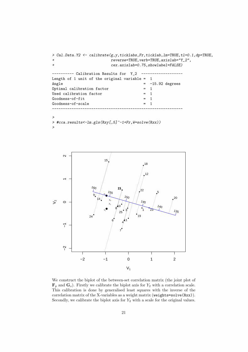
> Cal.Data.Y2 <- calibrate(g,y,ticklabs,Fr,ticklab,lm=TRUE,tl=0.1,dp=TRUE,

+ reverse=TRUE,verb=TRUE,axislab="Y_2",

+ cex.axislab=0.75,showlabel=FALSE)

---------- Calibration Results for Y_2 -------------------





Goodness-of-fit = 1


------------------------------------------------------------

>

> #cca.results<-lm.gls(Rxy[,5]~-1+Fr,W=solve(Rxx))

>

●

●

−2 −1 0 1 2

−2

−1

01

2

V1

V2

X1

X2

Y1

Y2

●

●

●

●

●

●

●

●

●

●

●

●

●

●

●

●

●

●

●

●

●

●

●

●

●

5

12

18

20

22

1

16

19

23

9

13

14

15

17

21

2

3

46

7

810

1124

25 135

140

145

150

155

160

We construct the biplot of the between-set correlation matrix (the joint plot ofFp and Gs). Firstly we calibrate the biplot axis for Y2 with a correlation scale.This calibration is done by generalised least squares with the inverse of thecorrelation matrix of the X-variables as a weight matrix (weights=solve(Rxx)).Secondly, we calibrate the biplot axis for Y2 with a scale for the original values.

21

This second calibration has no weight matrix and is obtained by ordinary leastsquares. Both calibrations have a goodness of fit of 1 and allow perfect recoveryof correlations and original data values.

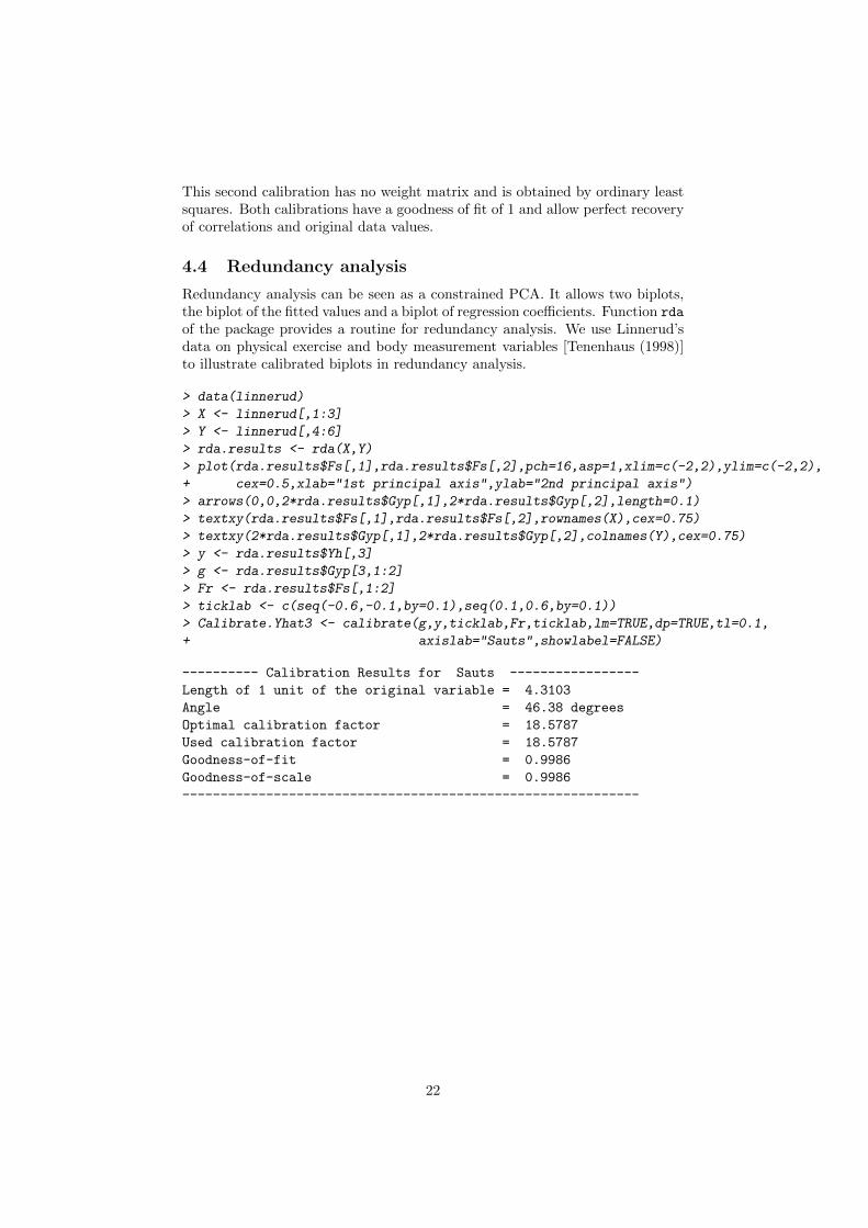
4.4 Redundancy analysis

Redundancy analysis can be seen as a constrained PCA. It allows two biplots,the biplot of the fitted values and a biplot of regression coefficients. Function rda

of the package provides a routine for redundancy analysis. We use Linnerud’sdata on physical exercise and body measurement variables [Tenenhaus (1998)]to illustrate calibrated biplots in redundancy analysis.

> data(linnerud)

> X <- linnerud[,1:3]

> Y <- linnerud[,4:6]

> rda.results <- rda(X,Y)

> plot(rda.results$Fs[,1],rda.results$Fs[,2],pch=16,asp=1,xlim=c(-2,2),ylim=c(-2,2),

+ cex=0.5,xlab="1st principal axis",ylab="2nd principal axis")

> arrows(0,0,2*rda.results$Gyp[,1],2*rda.results$Gyp[,2],length=0.1)

> textxy(rda.results$Fs[,1],rda.results$Fs[,2],rownames(X),cex=0.75)

> textxy(2*rda.results$Gyp[,1],2*rda.results$Gyp[,2],colnames(Y),cex=0.75)

> y <- rda.results$Yh[,3]

> g <- rda.results$Gyp[3,1:2]

> Fr <- rda.results$Fs[,1:2]

> ticklab <- c(seq(-0.6,-0.1,by=0.1),seq(0.1,0.6,by=0.1))

> Calibrate.Yhat3 <- calibrate(g,y,ticklab,Fr,ticklab,lm=TRUE,dp=TRUE,tl=0.1,

+ axislab="Sauts",showlabel=FALSE)

---------- Calibration Results for Sauts -----------------







------------------------------------------------------------

22

●

●

●

●

●

●

●

●

●

●

●

●

●

●●

●

●

●

●

●

−2 −1 0 1 2

−2

−1

01

2

1st principal axis

2nd

prin

cipa

l axi

s

8

10

11

12

13

18

19

20

5

9

15

2

417

1

3 6

7 16

Flexions

Sauts

Tractions

−0.6

−0.5

−0.4

−0.3

−0.2

−0.1

0.1

0.2

0.3

0.4

0.5

0.6

> plot(rda.results$Gxs[,1],rda.results$Gxs[,2],pch=16,asp=1,xlim=c(-2,2),

+ ylim=c(-2,2),cex=0.5,xlab="1st principal axis",

+ ylab="2nd principal axis")

> arrows(0,0,rda.results$Gxs[,1],rda.results$Gxs[,2],length=0.1)

> arrows(0,0,rda.results$Gyp[,1],rda.results$Gyp[,2],length=0.1)

> textxy(rda.results$Gxs[,1],rda.results$Gxs[,2],colnames(X),cex=0.75)

> textxy(rda.results$Gyp[,1],rda.results$Gyp[,2],colnames(Y),cex=0.75)

> y <- rda.results$B[,3]

> g <- rda.results$Gyp[3,1:2]

> Fr <- rda.results$Gxs[,1:2]

> ticklab <- seq(-0.4,0.4,0.2)

> W <-cor(X)

> Calibrate.Y3 <- calibrate(g,y,ticklab,Fr,ticklab,lm=TRUE,dp=TRUE,tl=0.1,

+ weights=W,axislab="Sauts",showlabel=FALSE)

---------- Calibration Results for Sauts -----------------






23


------------------------------------------------------------

> ticklab <- seq(-0.4,0.4,0.1)

> Calibrate.Y3 <- calibrate(g,y,ticklab,Fr,ticklab,lm=FALSE,tl=0.05,verb=FALSE,

+ weights=W)

> ticklab <- seq(-0.4,0.4,0.01)

> Calibrate.Y3 <- calibrate(g,y,ticklab,Fr,ticklab,lm=FALSE,tl=0.025,verb=FALSE,

+ weights=W)

●

●

●

−2 −1 0 1 2

−2

−1

01

2

1st principal axis

2nd

prin

cipa

l axi

s

Poids

Tourdetaille

Pouls

FlexionsSauts

Tractions

−0.4

−0.2

0

0.2

0.4

The first biplot shown is a biplot of the fitted values (obtained from the regres-sion of Y onto X). Vectors for the response variables are multiplied by a factorof 3 to increase readability. The fitted values of the regression of Sauts ontothe body measurements have a goodness of fit of 0.9984 and can very well berecovered by projection onto the calibrated axis. The second biplot is a biplot ofthe matrix of regression coefficients. We calibrated the biplot axis for ”Sauts”,such that the regression coefficients of the explanory variables with respect to”Sauts” can be recovered. The goodness of fit for ”Sauts” is over 0.99, whichmeans that the regression coefficients are close to perfectly displayed. Note thatthe calibration for Sauts for the regression coefficients is done by GLS withweight matrix equal to the correlation matrix of the X variables (weights=W).

24

5 Online documentation

Online documentation for the package can be obtained by typing vignette("CalibrationGuide"or by accessing the file CalibrationGuide.pdf in the doc directory of the in-stalled package.

6 Version history

Version 1.6:

� Function rad2degree and shiftvector have been added.

� Function calibrate has changed. Argument shift from previous versionsis obsolete, and replaced by shiftdir, shiftfactor and shiftvec.

Version 1.7.2:

� Function textxy has been modified and improved. Arguments dcol andcx no longer work, and their role has been taken over by col and cex. Anew argument offset controls the distance between point and label.

Acknowledgements

This work was partially supported by the Spanish grant BEC2000-0983. I thankHolland Genetics (http://www.hg.nl/), Janneke van Wagtendonk and Sanderde Roos for making the calves data available. This document was generated bySweave [Leisch (2002)].

References

[Anderson (1984)] Anderson, T. W. (1984) An Introduction to Multivariate Sta-tistical Analysis John Wiley, Second edition, New York.

[Frets (1921)] Frets, G. P. (1921) Heredity of head form in man, Genetica, 3,pp. 193-384.

[Gabriel, 1971] Gabriel, K. R. (1971) The biplot graphic display of matrices withapplication to principal component analysis. Biometrika 58(3) pp. 453-467.

[Gower and Hand (1996)] Gower, J. C. and Hand, D. J. (1996) Biplots Chap-man & Hall, London.

[Graffelman (2005)] Graffelman, J. (2005) Enriched biplots for canonical corre-lation analysis Journal of Applied Statistics 32(2) pp. 173-188.

[Graffelman and Aluja-Banet (2003)] Graffelman, J. and Aluja-Banet, T.(2003) Optimal Representation of Supplementary Variables in Biplots fromPrincipal Component Analysis and Correspondence Analysis BiometricalJournal, 45(4) pp. 491-509.

25

[Graffelman and van Eeuwijk (2005)] Graffelman, J. and van Eeuwijk, F. A.,(2005) Calibration of multivariate scatter plots for exploratory analysis ofrelations within and between sets of variables in genomic research, Biomet-rical Journal, 47, 6, 863-879.

[Leisch (2002)] Leisch, F. (2002) Sweave: Dynamic generation of statistical re-ports using literate data analysis Compstat 2002, Proceedings in Compu-tational Statistics pp. 575-580, Physica Verlag, Heidelberg, ISBN 3-7908-1517-9 URL http:/www.ci.tuwien.ac.at/ leisch/Sweave.

[Manly (1989)] Manly, B. F. J. (1989) Multivariate statistical methods: aprimer Chapman and Hall, London.

[Mardia et al.(1979)] Mardia, K. V. and Kent, J. T. and Bibby, J. M. (1979)Multivariate Analysis Academic Press London.

[R Development Core Team (2004)] R Development Core Team (2004) R: Alanguage and environment forstatistical computing. R Foundation for Sta-tistical Computing, Vienna, Austria, ISBN 3-900051-00-3, http://www.R-project.org.

[Tenenhaus (1998)] Tenenhaus, M. (1998) La Regression PLS Paris, EditionsTechnip.

[Venables and Ripley (2002)] Venables, W. N. and Ripley, B. D. (2002) ModernApplied Statistics with S-Plus New York, Fourth edition, Springer.

26

a guide to scatterplot and biplot calibration - the … · · 2015-02-19a guide to scatterplot...

Documents