1

International Conference on Ships and Offshore Structures

ICSOS 2017

11 – 13 September 2017, Shenzhen, China

A life-cycle cost model for the reliability-based design of

disconnectable FPSO mooring lines

José Manuel Cabrera-Mirandaa,b

, Patrícia Mika Sakugawac, Rafael

Corona-Tapiad, Jeom Kee Paik

a,b,e,*

aDepartment of Naval Architecture and Ocean Engineering, Pusan National University, Busan 46241, Republic of Korea bThe Korea Ship and Offshore Research Institute (The Lloyd’s Register Foundation Research Centre of Excellence), Pusan

National University, Busan 46241, Republic of Korea cDepartment of Mechanical Engineering & Post-Graduate Program in Science and Petroleum Engineering, University of

Campinas, Campinas, São Paulo, Brazil dInfraestructura y Evaluación, Coordinación de Diseño, Gerencia de Administración de Asignaciones en Aguas Profundas,

Bloques Norte, Pemex Exploración y Producción, Tampico 89000, Tamaulipas, México eDepartment of Mechanical Engineering, University College London, London WC1E 7JE, UK

Abstract

Floating production, storage, and offloading units (FPSOs) are widely used to develop offshore oil fields from

shallow to ultra-deep waters, and some possess fast disconnection systems to avoid harsh environmental conditions.

According to a literature survey, the current industry practice is based on the perceptions and experiences of

operators to judge the disconnection of these units during cyclonic storms. However, systematic criteria should be

established to judge whether disconnection is needed, and the downtime costs and safety issues associated with

life-cycle costs should be considered. In this paper, a life-cycle cost model is proposed to optimize (1) the

disconnection criteria of FPSOs and (2) the design of their mooring system. Relevant ultimate limit states and

reliabilities are considered in association with hull collapse, mooring system failure, and green water impact failure.

Effects of downtime costs (deferred production costs), mobilization, and other failure costs are considered.

Disconnection criteria are then formulated in terms of the significant wave height and wind speed limits. Because a

permanent mooring system may exhibit excessive resistance, it is possible to further optimize the life-cycle cost by

reducing the system’s resistance until an optimum reliability is obtained, minimizing the costs for non-permanent

service. An FPSO in the Gulf of Mexico is selected as an example to illustrate the application of the developed

model. The results of this study show that important savings for an overall FPSO project can be achieved by

implementing the proposed optimizations.

Keywords: disconnection criteria; FPSO; life-cycle cost; mooring system; target reliability index; ultimate limit state.

Nomenclature

random variable

ti period of deferred production (yr)

moor mooring system reliability index (-)

parameter of mooring system resistance

Γ vector of possible values for

DPiC cost of deferred production (USD)

EDiC cost of environmental damage (USD)

FC future cost (USD)

* Corresponding author. Tel.: +82 51 510 2429; fax: +82 51 518 7687.

E-mail address: jeompaik@pusan.ac.kr (JK Paik)

2

GiC general future cost (USD)

IC initial cost (USD)

LiC cost of life loss (USD)

MiC cost of mobilization (USD)

RiC cost of replacement (USD)

TC total life-cycle cost (USD)

ToptC optimum expected life-cycle cost (USD)

moorToptC

optimum expected life-cycle cost for an optimized mooring system (USD)

WiC cost of injuries or wounds (USD)

apd depletion rate at peak production (bbl·yr

-1)

E expected value

LH significant wave height limit (m)

LH vector of possible values for significant wave height limit

SH significant wave height (m)

j annual discount rate (yr-1

)

k net annual discount rate (yr-1

)

N number of broken mooring lines (-) t

q annual production rate (bbl·yr

-1)

P probability

fiP annual probability of failure for the i-th limit state (yr

-1)

fmoorP annual probability of failure of mooring system (yr

-1)

PVF present value function

R revenue stream (USD·yr-1

)

r inflation rate (yr-1

)

iR resistance for the i-th limit state

moorR mooring system resistance

swS

,1 still-water bending moment (N·m)

hogwvS

,1 hogging vertical wave-induced bending moment (N·m)

sagwvS

,1 sagging vertical wave-induced bending moment (N·m)

iS solicitation for the i-th limit state

T project life (yr)

t time (yr)

U wind speed (m·s-1

)

LU wind speed limit (m·s

-1)

LU vector of possible values for wind speed limit

1. Introduction

1.1. Preliminaries on disconnectable FPSOs

Floating production, storage, and offloading (FPSO) systems are a proven technology for the

development of deep offshore oil fields. Their wide area for topside allocation, large storage capacity

and adaptability for a wide range of water depths make them a feasible alternative for the production of

offshore oil fields from mild to harsh environments.

Some FPSOs with single-point mooring systems (SPMs) can be disconnected to avoid extreme

environmental loads, sail toward sheltered areas, and restart operations when the weather becomes

benign. The first moored FPSO with a disconnectable turret was introduced in West Australia in 1985,

and their use has since been extended to Australia, China, Canada (Mastrangelo et al. 2007), and the

Gulf of Mexico (Aanesland et al. 2007; Daniel et al. 2013). Disconnectable mooring systems have

several advantages in addition to lowering design loads; they reduce risk to asset damage, make the

production of lost infrastructure autonomous, and eliminate the need for helicopter evacuations (Daniel

et al. 2013). However, complex mechanisms require disconnection and reconnection, which increases

capital expenditure and operational expenditure (Shimamura 2002).

This paper focuses on the disconnection and design criteria for FPSO mooring systems. Several

design codes provide requirements for the classification and design of these systems. For example, API

(2001) requires floating production systems with fast disconnection systems to withstand the maximum

3

design conditions when the threshold environment for disconnection is reached. ABS (2014) and LR

(2016) define disconnectable units or systems as self-propelled floating units. DNV GL (2017) allows

offshore units to be classified as non–self-propelled. Nevertheless, it is outside the scope of these codes

to set any disconnection criteria.

Disconnectable SPMs for FPSOs can be classified into those with fast and regular disconnection

functions (Li et al. 2014). The former necessitate self-propulsion to achieve quick release and escape

from typhoons, cyclones, and hurricanes, and the latter are commonly designed for 100-yr return period

conditions. Examples of systems with a regular disconnection function can be seen in the South China

Sea, where this alternative has fit well with the construction and operating experience of operators (Li

et al. 2014), and in the Mexican Gulf of Mexico, where the mooring system of the FPSO for the

KuMaZa field is capable of withstanding hurricane conditions (Aanesland et al. 2007). There are two

FPSOs in the US Gulf of Mexico with fast disconnection functions. The FPSO for the Cascade and

Chinook fields is self-propelled, and her mooring system is designed to stay connected during 100-yr

return period winter storms but to disconnect during hurricanes (Mastrangelo et al. 2007; Daniel et al.

2013). Moreover, her disconnected buoy is designed for 1,000-yr return period loop/eddy currents.

Another FPSO in the US Gulf of Mexico, that for the Stones field, also has a fast disconnection

function (Leon 2016).

1.2. Previous research on life-cycle cost analysis of marine structures

Life-cycle cost analysis (LCCA) consists of adding the initial costs such as engineering, purchase,

fabrication, and installation costs to future costs such as failure, operation, maintenance, and

decommissioning costs. Early ideas about its use were proposed by Stahl (1986) for fixed offshore

structures and by Bea (1994) for crude-oil carriers. In 1994 and 1997, the International Ship and

Offshore Structures Congress (ISSC) adopted the LCCA or so-called economic criteria to evaluate the

safety level and risks of ship structures. The total cost of a structure can be expressed as

FFITCPCC , where

IC is the initial cost,

FP is the probability of failure over the expected

lifetime of the structure, and F

C is the failure cost (Béghin 2010).

Previous applications of LCCA have allowed the optimization of marine structures. For example, the

minimization of life-cycle costs has been used to derive reliability indices for the design of fixed

offshore structures (Stahl et al. 2000; Kübler & Faber 2004; Campos et al. 2013; Lee et al. 2016) and to

establish inspection plans to sustain the reliability index through the service life of these structures

(Moan 2011). Maintenance, repair, replacement, and mobilization of equipment costs have been

minimized to define a lower deck elevation for fixed offshore platforms (Campos et al. 2015). Bayesian

probabilistic network–based consequence models have been used to derive target reliability indices for

the design of FPSOs (Faber et al. 2012; Heredia-Zavoni et al. 2012). A multidisciplinary optimization

of vessel life-cycle cost with an enhanced multiple-objective collaborative optimizer was developed for

the design of naval ships (Temple & Collette 2017).

Marine operations can be also optimized by means of LCCA. The cost of safety improvement for

liquefied natural gas transfer arm operations was optimized by means of fuzzy logic with an evidential

reasoning algorithm (Nwaoha 2014). Ship oil-drain intervals have been planned by combining

oil-analysis program data interpretation and LCCA (Langfitt & Haselbach 2016). With the advent of

offshore wind energy, LCCA has been used to optimize vessel chartering strategies for the development

of offshore wind farms (Dalgic, Lazakis, Dinwoodie, et al. 2015; Dalgic, Lazakis, Turan, et al. 2015)

and to develop tools to evaluate wind farms’ life-cycle costs (Lagaros et al. 2015).

1.3. Objectives

The objective of this paper is to derive the target reliability index for the design of the lines in

disconnectable mooring systems. To achieve this, a method to define the limit metocean conditions at

which an FPSO should be disconnected by a life-cycle cost model is proposed. Then, said model is

implemented with expected future costs as a function of failure probability. Minimization of such costs

allows to derive an optimum disconnection criterion. Furthermore, a target reliability can be derived by

reducing the resistance of the system until the life-cycle cost is optimized.

The current condition for FPSO disconnection is the occurrence of cyclonic storms. Although

extensive research has been conducted on the life-cycle cost-based optimization of offshore structures,

to our knowledge, no attempt has been made to optimize the disconnection criteria. In this regard, this

4

paper offers a novel approach to determine the maximum environmental conditions that the mooring

system shall withstand as well as the criteria for a reliability-based design.

The remainder of this paper is organized as follows. In Section 2, the mathematical model to

calculate the expected life-cycle cost is presented, which allows to determine the limiting

environmental conditions for disconnection and define the target reliability index for the mooring

system. In Section 3, an applied example of an FPSO in the Gulf of Mexico is used to illustrate the

application. In Section 4, results are presented for the calculated disconnection criteria and mooring

system target reliability index. Finally, conclusions are given in Section 5.

2. A life-cycle cost model

The present value of the total life-cycle cost T

C of a structure is composed by the initial costs I

C

and future costs F

C . Its expected value can be expressed as

FIT

CECECE (1)

where E denotes the expected value.

The initial cost of a project is well known in comparison with future costs; therefore, II

CCE is

an acceptable approximation. We study the expected future costs due to failure and neglect the

failure-independent operational expenditure. Hence, Eq. (1) is rewritten as

fiiIT

PcCCE (2)

where i

c is the expected future cost for the i -th limit state as a function of its annual probability of

failure fi

P .

2.1. Components of future costs

A holistic approach is used by including economic, social, and environmental effects in the model as

advised by De Leon and Ang (2008). Each future cost, also known as failure cost or risk expenditure

(RISKEX), can then be written as

DPiEDiLiWiMiRifii

CECECECECECEPc (3)

where Ri

C is the cost of replacement, Mi

C is the cost of mobilization, Wi

C is the cost of injuries or

wounds, Li

C is the cost of life loss, EDi

C is the cost of environmental damage, and DPi

C is the cost

of deferred production.

Table 1. Assumptions for calculating failure costs.

Limit state Definition Assumptions

ULS hull midship section The acting vertical bending moment equals

or exceeds the hull ultimate strength

The whole FPSO must be replaced with the

exception of the subsea systems

ULS mooring system (one

line failure)

The acting tension equals or exceeds the

breaking load of one mooring line

One mooring line must be replaced

ULS mooring system (two

or more line failures)

The acting tension equals or exceeds the

breaking load of two or more mooring lines

FPSO drifts off of position, breaking subsea

umbilicals and risers

ULS green water at

accommodation area

Abnormal wave access to deck in

accommodation area

Damage to accommodation area

ULS green water not at

accommodation area

Abnormal wave access to deck in process

or utility areas

Damage to tanks and processing equipment

Disconnection FPSO is disconnected to avoid anticipated

extreme loads

FPSO is disconnected, mobilized to port under

self-propulsion, re-mobilized to site, and

reinstalled

Six limit states are included in the model: (I) the ultimate limit state (ULS) of the midship section

due to vertical bending moment, (II) the ULS of one mooring line, (III) the simultaneous ULS of two or

more mooring lines, (IV) green water at the area of accommodation, (V) green water at other areas, and

(VI) FPSO disconnection. The assumptions used to calculate the associated future costs are summarized

5

in Table 1. A thorough discussion of FPSO limit states is available in an HSE report (Noble Denton

Europe Ltd 2001).

Although limit states (II) and (III) could be considered parts of the same limit state, they have

different consequences. In fact, mooring systems that comply with API-2SK (API 2005) hold sufficient

redundancy to maintain position after one line failure, and therefore the division into two limit states is

realistic. Limit state (VI) does not have consequences for life, environment, or infrastructure; however,

important economic losses occur when the FPSO is disconnected. Hence, it is desirable to reduce the

downtime.

2.2. Expected future costs

The expected value of future costs is derived as in Stahl (1986). A general future cost Gi

C at time

t is estimated by means of the annual inflation rate r in the form of

rtCCGittGi

exp

(4)

where Gi

C is the equivalent cost of failure evaluated at 0t .

By bringing the future costs to the beginning of the project, Eq. (4) becomes

jtrtCCGitGi

expexp0

(5)

where j is the annual discount rate.

The expected cost can be estimated as the product of the present value cost and the probability of

experiencing that cost. Hence, the expected future cost can be expressed as

dtktPCCET

fiGiGi 0

exp (6)

where rjk is the net annual discount rate and T is the project life.

The expected future costs in Eq. (3) are readily obtained by solving the integral in Eq. (6), which

gives

PVFfiRiRi

PCCE (7)

PVFfiMiMi

PCCE (8)

PVFfiWiWi

PCCE (9)

PVFfiLiLi

PCCE (10)

PVFfiEDiEDi

PCCE (11)

where

kkT exp1PVF (12)

is the present value function.

The cost of deferred production necessitates different handling. If the FPSO fails at time t , the

deferred production cost under the assumption of replacement after failure equals

dtkRdtkRtCi

i

tT

tt

T

tDPi

expexp (13)

where tR is the revenue stream from the product exploitation at t and i

t is the period of

deferred production while the unit is out of service for the i -th limit state. Substitution of Eq. (13) into

(6) gives the expected cost of deferred production

.exp0

dtkttCPCET

DPifiDPi (14)

6

2.3. Probability of failure

Using the underscore to indicate random variables, the event that the FPSO is connected is defined

by the space LLSUUHH , where

SH is the random significant wave height,

LH is the

discrete significant wave height limit for disconnection, U is the random wind speed, and L

U is the

discrete wind speed limit for disconnection. Noting that the FPSO can only fail in the said space, the

probability of failure is written as

fi i i S L LP P S H H U U R (15)

where P denotes the probability, iS is the solicitation (load or demand), and i

R is the

resistance (strength or capacity) for the i -th limit state.

Regarding limit state (I) or the ULS of midship section due to the vertical bending moment, two

failure modes are possible: hogging and sagging bending moment failures. By using the appropriate

signs, Eq. (15) takes the form of

1 1, 1, 1, 1, 1, 1,0 0

f hog sw wv hog sag sw wv sag S L LP P S S S S H H U U

R R (16)

where hog,1

R is the hull ultimate strength in the hogging condition, sw

S,1

is the still-water bending

moment, hogwv

S,1

is the hogging vertical wave-induced bending moment, sag,1

R is the hull ultimate

strength in the sagging condition, and sagwv

S,1

is the sagging vertical wave-induced bending moment.

For the mooring system, each mooring line is a serial system composed of various sections. The failure

of one or more sections of the same line implicates the failure of that mooring line. The probability that

one mooring line is broken for limit state (II) is conveniently expressed as

21

f S L LP P N H H U U (17)

and the probability that two or more lines are broken for limit state (III) is

32

f S L LP P N H H U U (18)

where N is the number of broken lines.

The probability of green water at the accommodation area can be calculated as

4 40

f S L LP P S H H U U (19)

for limit state (IV). The probability of green water at other areas in limit state (V) is expressed as

5 50

f S L LP P S H H U U (20)

where 4S and 5

S represent the vertical relative motion of the deck with respect to the wave surface

at the accommodation area and other areas, respectively.

The failure space for limit state (VI) is the complement of the connected FPSO event space. Thus, it

is expressed as

6.

f S L LP P H H U U (21)

2.4. Optimum disconnection criteria

Eq. (15) indicates that the probability of failure is a function of the limit environmental conditions,

i.e., LLfifi

UHPP , . Let the vectors L

H and L

U contain possible values for L

H and L

U ,

respectively. Accordingly, the optimum expected life-cycle cost can be stated as

LL

UH ,minfiiITopt

PCCC (22)

which is associated with an optimum L

H and an optimum L

U .

7

2.5. Target reliability index for disconnectable mooring systems

Let Topt

C be a function of a second function that characterizes the mooring system resistance

moorR , i.e.,

moorToptToptCC R . Therefore, the optimization of

ToptC is made possible by solving

minTopt moor Topt

C C

Γ (23)

where moorTopt

C

is the optimum expected life-cycle cost for an optimized mooring system and Γ is the

vector of possible values for moor

R .

To determine Eq. (23), some variables must be expressed as functions of the mooring system

resistance. For this model, moorII

CC R , moorRR

CC R22

, moorMM

CC R22

,

moorRR

CC R33

, moorMM

CC R33

, moorff

PP R22

, and moorff

PP R33

. Possible

candidates for moor

R are the mooring line thickness, weight, line strength, and overall mooring

system strength. In Section 4.2, this function is taken as the minimum breaking load (MBL) of the top

mooring line section.

Because limit states (II) and (III) exclude each other, the probability of failure of the mooring

system fmoor

P is simply calculated as

32 fffmoor

PPP (24)

from which the mooring system reliability index moor

can be calculated. The latter is defined as

fmoormoor

P1 (25)

where 1 is the inverse standard normal cumulative distribution function.

The target moor

is the one associated with moorTopt

C

in Eq. (23) because this value minimizes the

life-cycle cost for a disconnectable FPSO.

2.6. Life-cycle cost-based optimization

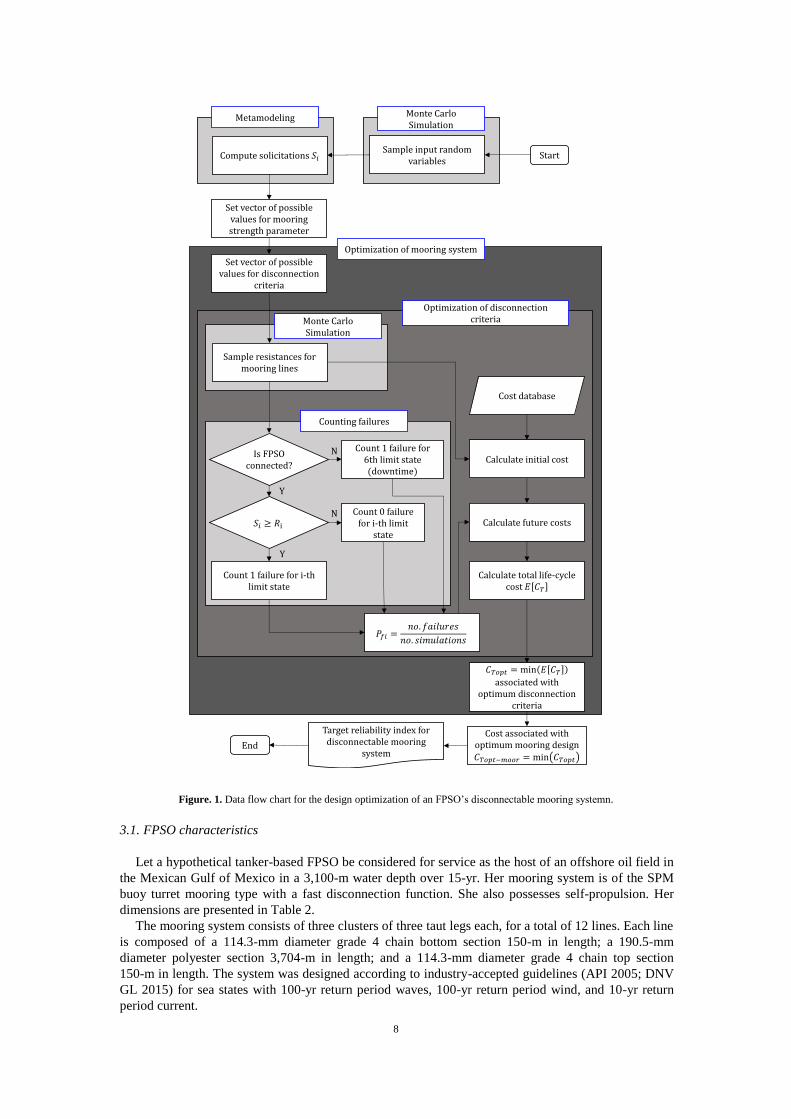
The proposed life-cycle cost model is implemented in a Matlab routine. Its algorithm is described by

Fig. 1. The first step is to carry out Monte Carlo simulation to sample the random resistances of the

different limit states and the random input variables for the solicitations.

Kriging metamodels are then used to estimate different solicitations on the FPSO with the ooDACE

Matlab toolbox (Couckuyt et al. 2010; Couckuyt et al. 2012; Ulaganathan et al. 2015). Metamodels are

approximate functions that serve to predict the responses of several input parameters. They require

design of computer experiments techniques such as Latin hypercube sampling (LHS) to establish

credible scenarios and feed the metamodels. A background on metamodel methods can be found in

Fang et al. (2006), and detailed information about their application in marine structures is documented

in the literature (Yang & Zheng 2011; Garrè & Rizzuto 2012; Cabrera-Miranda & Paik 2017).

The LCCA is conducted inside the disconnection criteria optimization loop, which is in turn

embedded into the mooring system optimization loop. Another Monte Carlo simulation is built in the

major loop to study the influence of the mooring system resistance. Finally, the optimum life-cycle

costs with associated disconnection criteria and mooring system reliability index are obtained as

outputs.

This approach assumes that the load remains unchanged after the mooring system’s resistance is

reduced. This is a conservative assumption, because a weak mooring system has less stiffness and

consequently a less static component of tension than a robust one.

3. Applied example

In this section, an example is used to illustrate the application of the proposed life-cycle cost model.

First, the floater characteristics are presented. To carry out the reliability analysis and determine the

failure probabilities, solicitations are investigated by means of a metamodel approach. Probabilistic

distributions for resistances are taken from the literature. Finally, the probabilities of failure are used to

estimate the expected value of the life-cycle cost.

8

Figure. 1. Data flow chart for the design optimization of an FPSO’s disconnectable mooring systemn.

3.1. FPSO characteristics

Let a hypothetical tanker-based FPSO be considered for service as the host of an offshore oil field in

the Mexican Gulf of Mexico in a 3,100-m water depth over 15-yr. Her mooring system is of the SPM

buoy turret mooring type with a fast disconnection function. She also possesses self-propulsion. Her

dimensions are presented in Table 2.

The mooring system consists of three clusters of three taut legs each, for a total of 12 lines. Each line

is composed of a 114.3-mm diameter grade 4 chain bottom section 150-m in length; a 190.5-mm

diameter polyester section 3,704-m in length; and a 114.3-mm diameter grade 4 chain top section

150-m in length. The system was designed according to industry-accepted guidelines (API 2005; DNV

GL 2015) for sea states with 100-yr return period waves, 100-yr return period wind, and 10-yr return

period current.

StartSample input random

variables

Monte Carlo Simulation

Metamodeling

Compute solicitations

Set vector of possible values for mooring strength parameter

Optimization of mooring system

Set vector of possible values for disconnection

criteria

Sample resistances for mooring lines

Monte Carlo Simulation

Counting failures

Is FPSO connected?

Count 1 failure for i-thlimit state

Count 1 failure for 6th limit state (downtime)

Count 0 failure for i-th limit

state

Calculate initial cost

Optimization of disconnection criteria

Calculate future costs

Calculate total life-cycle cost

associated with optimum disconnection

criteria

Cost associated with optimum mooring design

Target reliability index for disconnectable mooring

systemEnd

Cost database

Y

Y

N

N

9

Table 2. Main particulars of a hypothetical tanker-shaped FPSO.

Particular Dimension

Length between perpendiculars 239-m

Breadth 42-m

Depth 21-m

Dead weight 108,000-t

Total cargo capacity 107,000-m3 (680,000-bbl)

3.2. Solicitation metamodels

The LHS technique was applied to select 50 scenarios and investigate the solicitations as a function

of the environmental and functional conditions (see Table 3). The wave parameters were taken from

DNV (2014), and the wind and current distributions were derived from data in API (2007). The

directions of the environment were approximated by means of directional functions, and the vessel’s

draft was assumed to follow a uniform distribution.

Table 3. Probabilistic distribution of input variables for the solicitation metamodels.

Variable Unit Distribution

Significant wave height m Weibull ( =1.81, =1.47)

Zero-crossing wave period s Lognormal distribution (158.0

95.07.0S

H ,

1685.007.0 exp[S

H0312.0 ])

Wave direction angle with respect to peak direction rad Directional function ( s =5)

1-h average wind speed at 10 m above sea level m·s-1 Log-normal ( =0.61, =0.725)

Wind direction angle respect to peak direction rad Directional function ( s =5)

Current speed at surface m·s-1 Log-normal ( =−1.1187, =0.432)

Current direction angle respect to peak direction rad Directional function ( s =5)

Draft m Uniform (6.38,15.85)

Figure. 2. Time-domain series of FPSO responses of a typical scenario for (a) mooring line tension at the top chain section for

the most loaded line, (b) vertical wave-induced bending moment, and (c) deck vertical motion relative to the wave surface at the

bow.

10

Figure 3. Predicted solicitations by Kriging metamodels (variables not shown are set to their mean value) for (a) mooring line

tension at the top chain section of the most loaded line, (b) hogging vertical wave-induced bending moment, and (c) deck vertical

motion relative to the wave surface at the bow.

For each scenario, station-keeping analyses were conducted with ANSYS Aqwa in the time domain.

The irregular waves were defined by the Pierson-Moskowitz spectrum, the wind by the ISO spectrum,

and the current by a slab profile. Time series of responses, like those shown in Fig. 2, were obtained

and analyzed. For each scenario, we extracted the maximum mooring line tension; the maximum and

minimum vertical wave-induced bending moment for hogging and sagging, respectively; and the

minimum vertical relative motion at four locations at the deck.

The input variables and responses for each scenario were then used to build the metamodels. A few

of the predicted solicitations are plotted in Fig. 3. Overall, 42 metamodels were computed that consisted

of 36 tensions for mooring line sections, two vertical wave-induced bending moments for hogging and

sagging, and four vertical motions relative to the wave surface at the bow, aft, port, and starboard.

Initially, the metamodels were inaccurate for extreme loads, and therefore 10 additional scenarios were

uniformly sampled between the maximum values of the LHS and the 100-yr return period conditions to

improve the predictions of the metamodels. Furthermore, wind speed and its direction and current speed

and its direction were excluded from the models for bending moments to reduce the mean error. The

remaining solicitations were modeled as functions of the eight variables (see Table 3).

3.3. Reliability analysis

Reliability analysis aims to calculate the failure probability for a certain limit state. In addition to the

random solicitations predicted by metamodels, other random variables had to be considered. The

still-water bending moment in Table 4 is described via a bimodal distribution as proposed by Ivanov et

al. (2011). This consists of two truncated normal distributions that describe hogging and sagging as two

sides of one phenomenon. Huang and Moan (2005) demonstrated that FPSOs were sometimes operated

under still-water loads above the rule moment. Therefore, we used 1.3 times the design still-water

bending moment, as indicated in the Common Structural Rules (IACS 2012). Moments minima were

taken as 6% of the design moments. Furthermore, we used a coefficient of variation of 0.6 for both

hogging and sagging, which fell within the range of values in the second paper.

Table 4. Random variables for the reliability analysis.

Description Unit Distribution

Still-water bending moment N.m Bimodal from truncated normal for sagging ( =−1.347×109,

=8.08×108, lb =−2.57×109, ub =−1.19×108, sK =0.6) and truncated

normal for hogging ( =1.735×109, =1.04×109, lb =1.53×108,

ub =3.31×109, hK =0.4)

Ultimate hull girder strength in hogging N.m Log-normal ( =22.99, =0.09975)

Ultimate hull girder strength in sagging N.m Log-normal ( =22.797, =0.09975)

Ultimate strength for chain N Log-normal ( =16.2826, =0.0499)

Ultimate strength for polyester rope N Log-normal ( =16.1148, =0.0499)

11

Figure 4. PDF of resistances (dot-dashed line) and solicitations (continuous line) for FPSO limit states without disconnection: (a)

hogging bending moment, (b) sagging bending moment, (c) tension at top-chain section of most loaded line, (d) tension at

intermediate polyester section of most loaded line, (e) green water at accommodation, (f) green water at bow, (g) significant

wave height and optimum disconnection limit, (h) wind speed and optimum disconnection criterion.

Figure 5. Probabilities of failure as function of (a) significant wave height limit and (b) wind speed limit.

Resistances for hull and mooring lines are usually assumed to follow a log-normal distribution. Their

parameters for this study are indicated in Table 4. The mean of the former was taken as the ultimate

strength of a tanker of similar dimensions with half corrosion addition in Kim et al. (2014). The

coefficient of variation was taken as 0.1, as suggested by Sun and Bai (2001). The parameters for the

resistance of mooring lines were taken from Vazquez-Hernandez et al. (2006).

The reliability analysis was carried out using the Monte Carlo simulation method with 1 × 106

simulations for a total of 47 random variables, some of which were used to estimate solicitations. Fig. 4

displays a comparison of the probability density functions (PDFs) for solicitations and resistances.

Afterward, limit state violations were evaluated, and the failure probabilities were then estimated. In

Fig. 5, the later ones are calculated as functions of an arbitrary single disconnection criterion, where

LH and LU are normalized with respect to the 100-yr return period significant wave height 100H

and 100-yr return period 1-hour average wind speed 100U , respectively. They in turn correspond to

10.13 m and 48 m/s, respectively.

No failure scenarios were found for limit states (II) and (III); thus, we conclude that 6

2101

fP

and 6

3101

fP . This can be better understood by examining the wide safety margin between

solicitations and resistances in Fig. 4(c) and (d).

12

3.4. Life-cycle cost analysis

Initial and future costs for replacement and reposition were calculated by means of QUE$TOR, a

capital expenditure/operational expenditure cost estimation software for oil and gas projects (IHS

Markit 2017). Wounds, life loss, and environmental damage costs were estimated based on local

regulations. Table 5 summarizes the equivalent costs of failure in normalized fashion with respect to the

initial cost of the project. The net annual discount rate was taken as 12% for the economical evaluation.

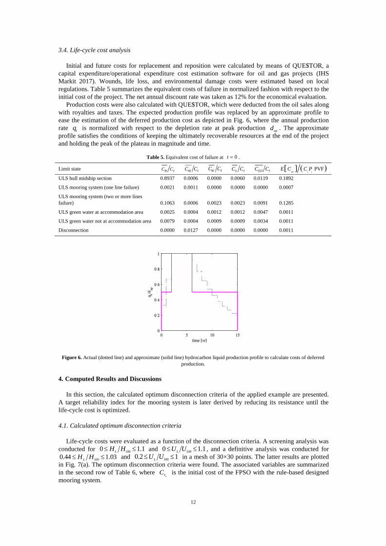
Production costs were also calculated with QUE$TOR, which were deducted from the oil sales along

with royalties and taxes. The expected production profile was replaced by an approximate profile to

ease the estimation of the deferred production cost as depicted in Fig. 6, where the annual production

rate t

q is normalized with respect to the depletion rate at peak production ap

d . The approximate

profile satisfies the conditions of keeping the ultimately recoverable resources at the end of the project

and holding the peak of the plateau in magnitude and time.

Table 5. Equivalent cost of failure at 0t .

Limit state IR CC IM CC IW CC IL CC IED CC PVFDP I f

E C C P

ULS hull midship section 0.8937 0.0006 0.0000 0.0060 0.0119 0.1892

ULS mooring system (one line failure) 0.0021 0.0011 0.0000 0.0000 0.0000 0.0007

ULS mooring system (two or more lines

failure) 0.1063 0.0006 0.0023 0.0023 0.0091 0.1285

ULS green water at accommodation area 0.0025 0.0004 0.0012 0.0012 0.0047 0.0011

ULS green water not at accommodation area 0.0079 0.0004 0.0009 0.0009 0.0034 0.0011

Disconnection 0.0000 0.0127 0.0000 0.0000 0.0000 0.0011

Figure 6. Actual (dotted line) and approximate (solid line) hydrocarbon liquid production profile to calculate costs of deferred

production.

4. Computed Results and Discussions

In this section, the calculated optimum disconnection criteria of the applied example are presented.

A target reliability index for the mooring system is later derived by reducing its resistance until the

life-cycle cost is optimized.

4.1. Calculated optimum disconnection criteria

Life-cycle costs were evaluated as a function of the disconnection criteria. A screening analysis was

conducted for 1.10100 HH

L and 1.10

100 UU

L, and a definitive analysis was conducted for

03.144.0100 HH

L and 12.0

100 UU

L in a mesh of 30×30 points. The latter results are plotted

in Fig. 7(a). The optimum disconnection criteria were found. The associated variables are summarized

in the second row of Table 6, where 0I

C is the initial cost of the FPSO with the rule-based designed

mooring system.

13

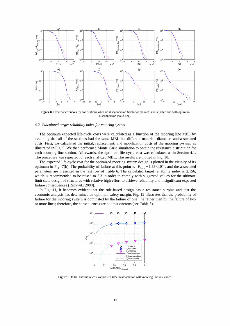
In Fig. 8, the exceedance curves demonstrate that most of the solicitations are reduced after the

optimum disconnection criteria are implemented. Exceptions include the relative vertical motions for

green water limit states (IV) and (V) in Fig. 8(e) and (f), respectively, where disconnection has little

influence.

Figure 7. Expected life-cycle cost for FPSO with (a) a rule-based designed mooring system and (b) an optimized mooring

system (optimum is shown as red point).

Table 6. Calculated optimum disconnection criteria and mooring system reliability index.

Case LH LU 6fP

(downtime

per yr)

0IT CCE

without

disconnection

0ITopt CC moor with

optimum

disconnection

FPSO with rule-based

designed mooring

system

5.5345 m 48 m/s 0.0057 1.0017 1.0009 >4.7534

FPSO with optimized

disconnectable mooring

system

5.5345 m 48 m/s 0.0057 0.9822 0.9816 2.156 (target)

14

Figure 8. Exceedance curves for solicitations when no disconnection (dash-dotted line) is anticipated and with optimum

disconnection (solid line).

4.2. Calculated target reliability index for mooring system

The optimum expected life-cycle costs were calculated as a function of the mooring line MBL by

assuming that all of the sections had the same MBL but different material, diameter, and associated

costs. First, we calculated the initial, replacement, and mobilization costs of the mooring system, as

illustrated in Fig. 9. We then performed Monte Carlo simulation to obtain the resistance distribution for

each mooring line section. Afterwards, the optimum life-cycle cost was calculated as in Section 4.1.

The procedure was repeated for each analyzed MBL. The results are plotted in Fig. 10.

The expected life-cycle cost for the optimized mooring system design is plotted in the vicinity of its

optimum in Fig. 7(b). The probability of failure at this point is 21055.1

fmoorP , and the associated

parameters are presented in the last row of Table 6. The calculated target reliability index is 2.156,

which is recommended to be raised to 2.3 in order to comply with suggested values for the ultimate

limit state design of structures with relative high effort to achieve reliability and insignificant expected

failure consequences (Rackwitz 2000).

In Fig. 11, it becomes evident that the rule-based design has a resistance surplus and that the

economic analysis has determined an optimum safety margin. Fig. 12 illustrates that the probability of

failure for the mooring system is dominated by the failure of one line rather than by the failure of two

or more lines; therefore, the consequences are not that onerous (see Table 5).

Figure 9. Initial and future costs at present time in association with mooring line resistance.

15

Figure 10. Optimum life-cycle cost and associated variables in association with mooring line resistance.

Figure 11. Comparison of PDF for solicitation and resistance for rule-based designed mooring system and optimized mooring

system.

Figure 12. Probabilities of failure for optimum mooring system as a function of (a) significant wave height limit and (b) wind

speed limit.

5. Conclusions

The industry practice on disconnectable FPSOs consists of disconnecting said units when cyclonic

storms approach and designing mooring systems for 100-yr return period non-cyclonic storms

according to API-RP-2SK. However, it is highly desirable to establish a systematic procedure to derive

disconnection and design criteria based on a cost-effective decision.

The objective of the present study has been to derive a target reliability index for the design of

mooring lines of disconnectable FPSOs. Said goal has been fulfilled by means of a proposed life-cycle

cost model which can be used to optimize the disconnection criteria for FPSOs and subsequently to

obtain a design criteria under reliability format.

16

A hypothetical tanker shaped FPSO was used to illustrate the application of the model. The

calculated target reliability index for the disconnectable mooring system is 2.156 and the limit

significant wave height is 5.35 m. Wind speed was found not to be a dominant parameter for the

minimization of failure costs for this problem.

Main contributions of this research are: (1) the provision of a life-cycle model for disconnectable

FPSO projects that serves as a framework for optimization of the disconnection and design criteria of

mooring systems (2) as well as an algorithm for its implementation. Moreover, the results of the applied

example show that savings of up to 2.01% of the initial cost of the project can be achieved if the

optimization of the mooring system design is carried out (see Table 6). Although these features cannot

be generalized, we expect other FPSO projects to cut production costs if the proposed optimizations are

used.

There is one important limitation in the implementation of the optimum disconnection criteria.

Although cyclonic-storms can be well predicted in advance, extra-tropical storms tend to develop

quickly, and therefore it is difficult or impossible to initiate a planned disconnection. Thus, the

distinction between the two types of said storms would offer an appreciable improvement for the

current life-cycle cost model and algorithm.

Acknowledgements

This study was undertaken at the Korea Ship and Offshore Research Institute at Pusan National

University which has been a Lloyd’s Register Foundation (LRF) Research Centre of Excellence since

2008. The authors are grateful to Dr. Alberto Omar Vazquez-Hernandez of the Mexican Petroleum

Institute (IMP) for his valuable discussion on the design of mooring systems. The first author would

like to acknowledge the scholarship from the Mexican National Council for Science and Technology

(CONACYT). The second author wishes to thank the financial support of PRH-15 ANP program.

References

Aanesland V, Kaalstad JP, Bech A, Holm A, Production NF. 2007. Disconnectable FPSO—Technology

To Reduce Risk in GoM. In: Offshore Technol Conf. Houston, USA; p. OTC 18487.

[ABS] American Bureau of Shipping. 2014. Rules for building and classing Floating Production

Instalations. Houston, USA.

[API] American Petroleum Institute. 2001. Recommended Practice for Planning, Designing, and

Constructing Floating Production Systems, API Recommended Practice 2FPS. First. Washington,

D.C.

[API] American Petroleum Institute. 2005. Design and Analysis of Stationkeeping Systems for Floating

Structures Recommended Practice 2SK. Third. Washington, D.C.

[API] American Petroleum Institute. 2007. Interim Guidance on Hurrican Conditions in the Gulf of

Mexico API Bulletin 2INT-MET. Washington, D.C.

Bea RG. 1994. Evaluation of Alternative Marine Structural Integrity Programs. Mar Struct. 7:77–90.

Béghin D. 2010. Reliability-Based Structural Design. In: Hughes OF, Paik JK, editors. Sh Struct Anal

Des. Jersey City, New Jersey: The Society of Naval Architects and Marine Engineers; p. 5-1-5–

63.

Cabrera-Miranda JM, Paik JK. 2017. On the probabilistic distribution of loads on a marine riser. Ocean

Eng. 134:105–118.

Campos D, Cabrera Miranda JM, Martínez Mayorga JM, García Tenorio M. 2013. Optimal Metocean

Design of Offshore Tower Structures. In: Proc ASME 2013 32nd Int Conf Ocean Offshore Arct

Eng OMAE2013. Nantes, France: ASME; p. OMAE2013-10953.

Campos D, Ortega C, Alamilla JL, Soriano A. 2015. Selection of Design Lower Deck Elevation of

Fixed Offshore Platforms for Mexican Code. J Offshore Mech Arct Eng. 137:51301-1-51301–8.

Couckuyt I, Declercq F, Dhaene T, Rogier H, Knockaert L. 2010. Surrogate-Based Infill Optimization

17

Applied to Electromagnetic Problems. Int J RF Microw Comput Eng. 20:492–501.

Couckuyt I, Forrester A, Gorissen D, De Turck F, Dhaene T. 2012. Blind Kriging: Implementation and

performance analysis. Adv Eng Softw. 49:1–13.

Dalgic Y, Lazakis I, Dinwoodie I, McMillan D, Revie M, Majumder J. 2015. Cost benefit analysis of

mothership concept and investigation of optimum chartering strategy for offshore wind farms.

Energy Procedia. 80:63–71.

Dalgic Y, Lazakis I, Turan O, Judah S. 2015. Investigation of optimum jack-up vessel chartering

strategy for offshore wind farm O & M activities. Ocean Eng. 95:106–115.

Daniel J, Mastrangelo CF, Ganguly P. 2013. First Floating , Production Storage and Offloading vessel

in the U.S. Gulf of Mexico. In: Offshore Technol Conf. Houston, USA; OTC 24112.

[DNV] Det Norske Veritas AS. 2014. Recommended practice DNV-RP-C205, Environmental

Conditions and Environmental Loads. [place unknown].

DNV GL. 2015. Offshore Standard DNVGL-OS-E301, Position mooring. [place unknown].

DNV GL. 2017. Rules for Classification, Offshore units, DNVGL-RU-OU-0102 Floating production,

storage and loading units. [place unknown].

Faber MH, Straub D, Heredia-Zavoni E, Montes-Iturrizaga R. 2012. Risk assessment for structural

design criteria of FPSO systems. Part I: Generic models and acceptance criteria. Mar Struct.

28:120–133.

Fang K, Li RZ, Sudjianto A. 2006. Design and modeling for computer experiments. Boca Raton, FL,

USA: Chapman & Hall/CRC.

Garrè L, Rizzuto E. 2012. Bayesian networks for probabilistic modelling of still water bending moment

for side-damaged tankers. Ships Offshore Struct. 7:269–283.

Heredia-Zavoni E, Montes-Iturrizaga R, Faber MH, Straub D. 2012. Risk assessment for structural

design criteria of FPSO systems. Part II: Consequence models and applications to determination

of target reliabilities. Mar Struct. 28:50–66.

Huang W, Moan T. 2005. Combination of global still-water and wave load effects for reliability-based

design of floating production, storage and offloading (FPSO) vessels. Appl Ocean Res. 27:127–

141.

IHS Markit. 2017. QUE$TOR

(https://www.ihs.com/products/questor-oil-gas-project-cost-estimation-software.html).

[IACS] International Association of Classification Societies. 2012. Common Structural Rules for Oil

Tankers. [place unknown].

Ivanov LD, Ku A, Huang B-Q, Krzonkala VCS. 2011. Probabilistic presentation of the total bending

moments of FPSOs. Ships Offshore Struct. 6:45–58.

Kim DK, Kim HB, Zhang X, Li CG, Paik JK. 2014. Ultimate strength performance of tankers

associated with industry corrosion addition practices. Int J Nav Archit Ocean Eng. 6:507–528.

Kübler O, Faber MH. 2004. Optimality and Acceptance Criteria in Offshore Design. J Offshore Mech

Arct Eng. 126:258–264.

Lagaros ND, Karlaftis MG, Paida MK. 2015. Stochastic life-cycle cost analysis of wind parks. Reliab

Eng Syst Saf. 144:117–127.

Langfitt Q, Haselbach L. 2016. Coupled oil analysis trending and life-cycle cost analysis for vessel

oil-change interval decisions interval decisions. J Mar Eng Technol. 15:1–8.

Lee S, Jo C, Bergan P, Pettersen B, Chang D. 2016. Life-cycle cost-based design procedure to

determine the optimal environmental design load and target reliability in offshore installations.

18

Struct Saf. 59:96–107.

Leon A. 2016. Breaking new frontiers. Offshore Eng Sept.:22–25.

De Leon D, Ang AHS. 2008. Confidence bounds on structural reliability estimations for offshore

platforms. J Mar Sci Technol. 13:308–315.

Li D, Yi C, Xu Z, Bai X. 2014. Scenario Research and Design of FPSO in South China. In: Proc

Twenty-fourth Int Ocean Polar Eng Conf. Vol. ISOPE-I-14. Busan, Korea: International Society

of Offshore and Polar Engineers (ISOPE); p. 964–969.

[LR] Lloyd’s Register. 2016. Rules and Regulations for the Classification of Offshore Units. London:

Lloyd’s Register Group Limited.

Mastrangelo C, Barwick K, Fernandes L, Theisinger E. 2007. FPSOs in the Gulf of Mexico

[presentation material]. In: Inf Transf Meet. Kenner, Louisiana, USA.

Moan T. 2011. Life-cycle assessment of marine civil engineering structures. Struct Infrastruct Eng.

7:11–32.

Noble Denton Europe Ltd. 2001. Rationalisation of FPSO design issues—Relative reliability levels

achieved between different FPSO limit states. Norwich: Health & Safety Executive.

Nwaoha TC. 2014. Inclusion of hybrid algorithm in optimal operations of liquefied natural gas transfer

arm under uncertainty. Ships Offshore Struct. 9:514–524.

Rackwitz R. 2000. Optimization — the basis of code-making and reliability verification. Struct Saf.

22:27–60.

Shimamura Y. 2002. FPSO/FSO : State of the art. J Mar Sci Technol. 7:59–70.

Stahl B. 1986. Reliability Engineering and Risk Analysis. In: McClelland B, Reifel MD, editors. Plan

Des fixed offshore platforms. New York: Van Nostrand Reinhold Company; p. 59–98.

Stahl B, Aune S, Gebara JM, Cornell CA. 2000. Acceptance Criteria for Offshore Platforms. J Offshore

Mech Arct Eng. 122:153.

Sun H-H, Bai Y. 2001. Time-Variant Reliability of FPSO Hulls. SNAME Trans. 109:341–366.

Temple D, Collette M. 2017. Understanding lifecycle cost trade-offs for naval vessels: minimising

production, maintenance, and resistance. Ships Offshore Struct. 12:756–766.

Ulaganathan S, Couckuyt I, Deschrijver D, Laermans E, Dhaene T. 2015. A Matlab toolbox for Kriging

metamodelling. Procedia Comput Sci. 51:2708–2713.

Vazquez-Hernandez AO, Ellwanger GB, Sagrilo LVS. 2006. Reliability-based comparative study for

mooring lines design criteria. Appl Ocean Res. 28:398–406.

Yang HZ, Zheng W. 2011. Metamodel approach for reliability-based design optimization of a steel

catenary riser. J Mar Sci Technol. 16:202–213.