a markov yield curve model -...
TRANSCRIPT

Quant History
Quant Factory Symposium
Aarhus
January 2014
Jesper Andreasen
Danske Markets, Copenhagen

2
Outline
Background: my CV and my job.
The good old days: the 90s.
The industrial period: 2000-2007.
The financial crisis: 2007-2008.
The aftermath: 2008-2013.
The Danske experience.
Conclusion.
3
References
Andreasen, J (2003): “Derivatives – the View from the Trenches.”
Presentation, Copenhagen University.
Andreasen, J (2013): “Option Anatomy.” Presentation, Copenhagen
University.
4
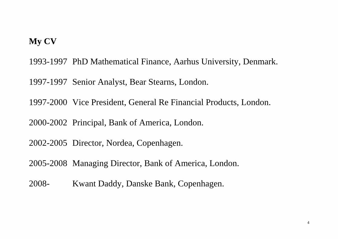
My CV
1993-1997 PhD Mathematical Finance, Aarhus University, Denmark.
1997-1997 Senior Analyst, Bear Stearns, London.
1997-2000 Vice President, General Re Financial Products, London.
2000-2002 Principal, Bank of America, London.
2002-2005 Director, Nordea, Copenhagen.
2005-2008 Managing Director, Bank of America, London.
2008- Kwant Daddy, Danske Bank, Copenhagen.
5
Job Description
Develop and implement pricing and hedging models for exotic and vanilla
derivatives in all asset classes.
... including the pricing of CVA and other 3-letter things.
Ad-hoc assistance with pricing and hedging problems.
IT and system implementation.
Fundamental research: Option pricing and hedging, yield curve models,
numerical methods, IT implementation, etc.
Team management.
6
The History of Quant
The history of quant can be broken into the following periods:
1. The Good Old Days: The 90s
2. The Industrialisation: 2000-2007
3. The Financial Crisis: 2007-2008
4. The Aftermath: 2008-now
In the following I will give my account of what happened.
... and what I think we can learn from it.
7
The Good Old Days – the 90s
The academic research of the 70s and 80s had laid out a strong theoretical
foundation for derivatives pricing in complete markets:
Black-Scholes-Merton (1973), Vasicek (1977), HJM (1989)
This was augmented with more strong results in the early 90s:
Jamshidian (1990), Dupire (1994), Heston (1993), BGM (1997)
This laid out a strong foundation. It was, however, the arrival of the first
interest rate swaps in the early 90s and the serious use of computers that
really changed the business.
8
When I started in 1997, Gen Re was running its entire portfolio on 4 CPUs
on a VMS mainframe.
Within a few years we were running on several hundreds of computers.
Black-Scholes and binomial trees were replaced by the non-central chi-
square, finite-difference methods, and Monte-Carlo simulation.
Ad-hoc pricing in spreadsheets was replaced with scripting languages for
general pay-offs.
As an example, during my Gen Re days (1997-2000) we implemented:
1. CEV pricing of all vanilla interest rate options.
2. CEV Cheyette model for Bermudans.
3. 3 factor (+ time) finite difference models for PRDCs.

9
4. BGM model with CEV skew.
5. Local volatility + jump model for equity and fx.
6. A scripting language called SynTech.
These developments were driven by a generation of young quants, that not
only understood the mathematics of the models, but also had an idea of how
to get it working on a computer.
Remember, that this generation had grown up with programming games on
ZX81s and Commodore 64s.
Our skill set was further improved by lots of hands-on practical development
and ad-hoc pricing of various exotic structures.
... plus, of course, first-hand experience of various f..k-ups.

10
Anecdote.

11
Lessons from the 90s
There were quant and model related losses in the 90s. Not whale size, but
still worth learning from.
One of the sins was ignorance of smiles and skews and inability or
willingness to calibrate to market data.
Many banks had losses on Bermuda swaptions and other dynamic rate
products because they didn’t use yield curves models with arbitrage free
dynamics.
So model builders that were too clever to calibrate or too smart to follow
established theory.

12
What Happens if You don’t Calibrate?
Assume zero rates and dividends and standard frictionless markets.
Assume that the underlying stock evolves continuously, i.e. that there exists
processes , so that under “real” measure:
( ) ( ) ( )ds t t dt t dW
Let V be the value of an option book on priced with constant volatility .
Assuming that the book is continuously delta hedged, i.e. we dynamically
trade the stock to keep 0sV , then the value of the option book will evolve
according to
13
2
2 2 2
012
1 1( )2 2
ss
s ss sst
V
dV V dt V ds V ds V dt
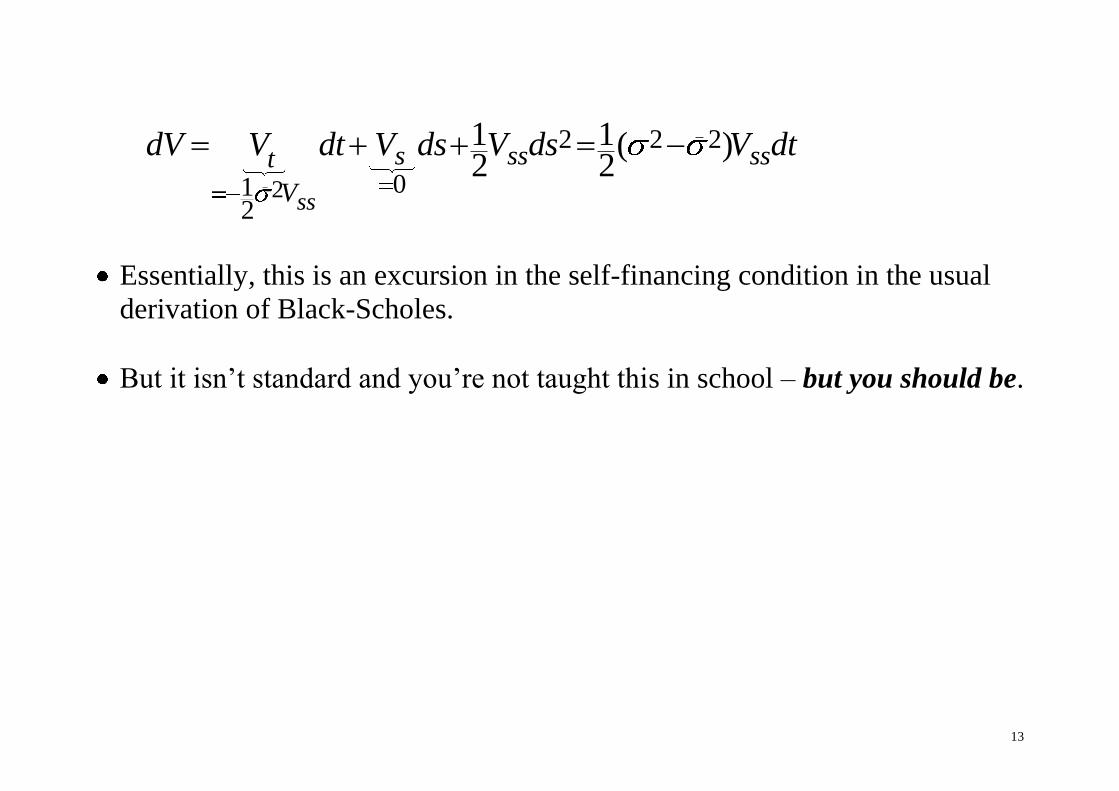
Essentially, this is an excursion in the self-financing condition in the usual
derivation of Black-Scholes.
But it isn’t standard and you’re not taught this in school – but you should be.
14
Implications for Trading
So you’re gamma long, 0ssV , and realised volatility is higher than the
pricing volatility, you make money.
The option trader’s job is really about balancing realised against implied (or
pricing) volatility:
1. Realised vol > implied vol => go long gamma
2. Realised vol < implied vol => go short gamma
In essence this is what all trading is about: buy low – sell high.
Unfortunately, easier said than done.
15
Implications for Models
The general point is that if your model, , is misspecified, you’re going to
make daily losses of ( )O dt not ( )O dW .
So contrary to common belief: bad models don’t blow up your books – they
bleed them to death.
It can take you a while before you realise that your model is wrong.
That is, you can pile up a lot of trades, make a lot of “model value”, and
many fine bonuses can be paid, before you realise that your book is
bleeding.
16
... and this has, involuntarily and independently, been discovered by many
banks.
17
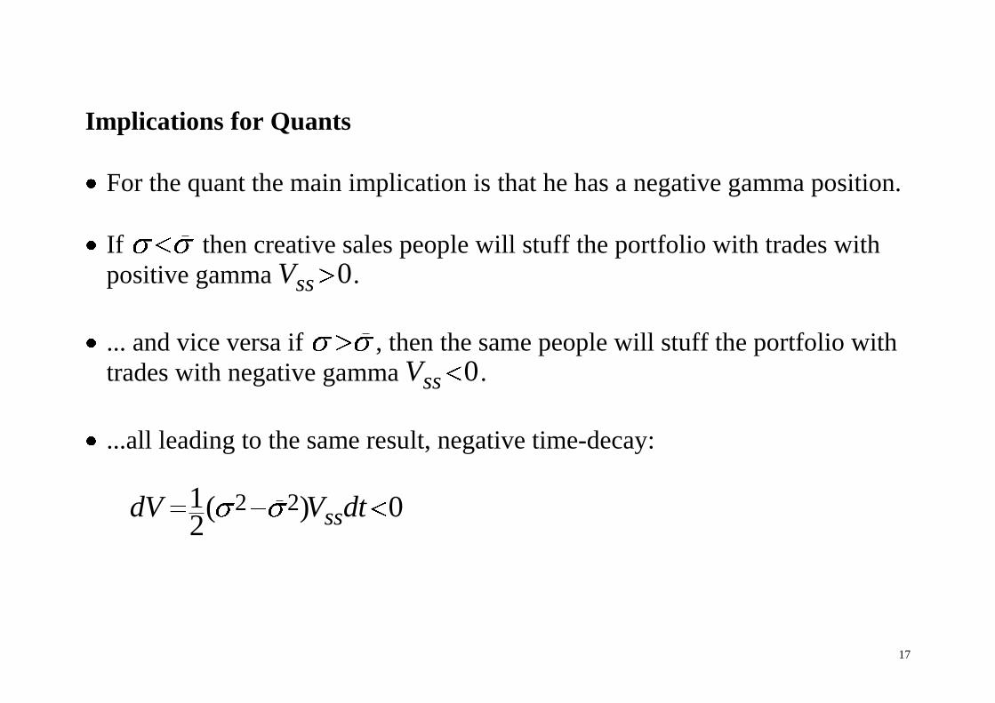
Implications for Quants
For the quant the main implication is that he has a negative gamma position.
If then creative sales people will stuff the portfolio with trades with
positive gamma 0ssV .
... and vice versa if , then the same people will stuff the portfolio with
trades with negative gamma 0ssV .
...all leading to the same result, negative time-decay:
2 21( ) 02 ssdV V dt
18
So the quant needs to walk the fine line , for his bank to stay in
business.
Measures:
1. Calibration: make sure that the model matches relevant market
prices, because implied volatility is the best forecast of realised.
2. Compare the prices of your model to bigger (better and slower)
models.
3. Study the literature, not only Hull’s book.
4. Experiment.
5. Write public papers, participate in conferences.
19
The Industrial Period – 2000-2007
Massive increase of scale in the derivatives industry -- particularly exotics.
Development of the “industrial” quant and the associated machinery:
1. Scripting languages for generic payoffs.
2. Structured model libraries with a strict model hierarchy: linear,
European option, and dynamic models.
3. Integrated calibration and risk machinery.
4. Highly structured C++ code.
Do you learn about code structure in school? You should.

20
We were now running portfolios of 1000s of exotic trades on 1000s of
computers.
Models that I worked on during this period include
1. Heston and SABR models for vanilla options.
2. Cheyette model for Bermuda swaptions.
3. 3-4 factor models for PRDCs.
4. Multi factor Cheyette model for interest rate derivatives.
5. Stochastic volatility + jump models for FX and equities.
6. The Beast: multi ccy and multi asset MFC + SVJ model.
7. ... used for hybrids and CVA.
8. Complete derivatives library from scratch at Nordea 2002-2005.
21
After a While It Started to a Smell a Bit ...
Shrinking margins due to increased competition.
Markets getting increasingly skewed.
In the 90s we had been able to sell PRDCs and getting the Bermuda call
right for free, now 3 factor models were not even adequate.
Skew on the FX and correlation had to be considered.
There seems to be a vicious circle in this:
increased competition
=> smaller margins
=> more complicated payoffs
22
=> piling on of unhedged esoteric risks
=> distortion of underlying market dynamics from delta hedging
=> more skewed markets
=> break-down of conventional models and
=> need for constant refinement of models.
23
The Financial Crisis 2007-2008
Early 2007: jitter in the US subprime market.
ITraxx CDS spreads widened from 30 bps to 90 bps during the summer of
2007 and credit spread volatility sky rocketed.
The interbank market broke down: banks did not trust each other.
Libor spreads, 1m-3m, 3m-6m, 6m-12m spreads widened dramatically as
early as summer 2007.
Conventional swap models did not account for this.
The 30-10 year spread on the yield curves (EUR and USD) inverted early
2008 and volatility of the long rates went wild.
24
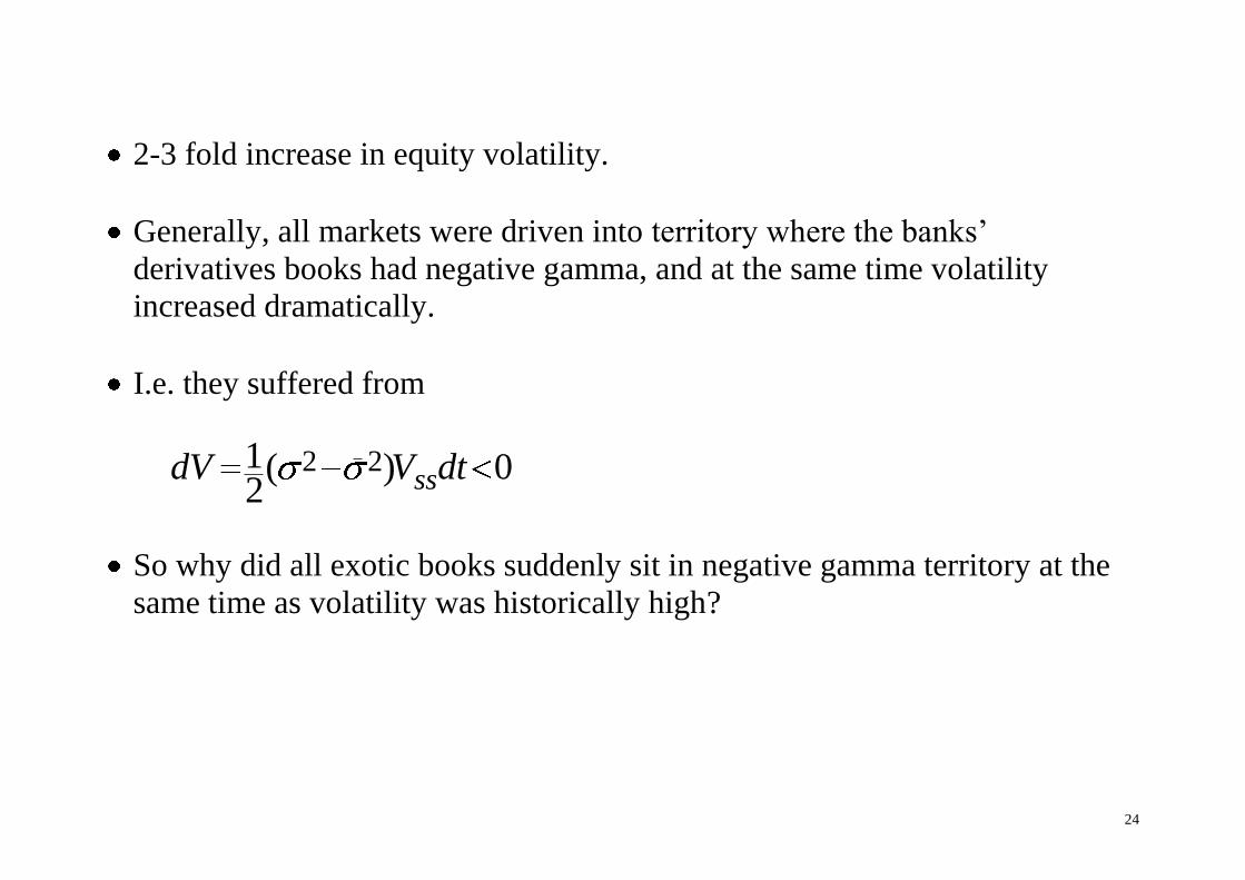
2-3 fold increase in equity volatility.
Generally, all markets were driven into territory where the banks’
derivatives books had negative gamma, and at the same time volatility
increased dramatically.
I.e. they suffered from
2 21( ) 02 ssdV V dt
So why did all exotic books suddenly sit in negative gamma territory at the
same time as volatility was historically high?
25
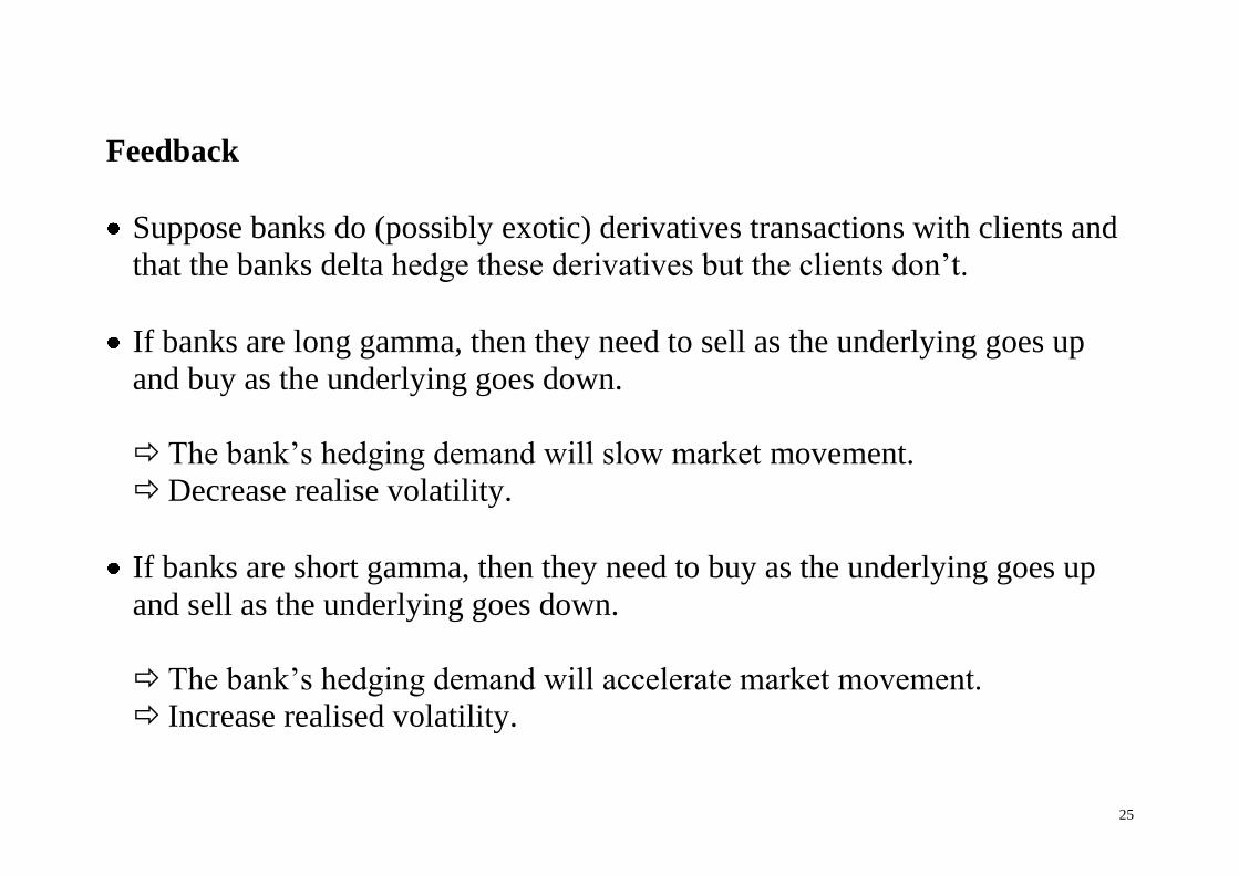
Feedback
Suppose banks do (possibly exotic) derivatives transactions with clients and
that the banks delta hedge these derivatives but the clients don’t.
If banks are long gamma, then they need to sell as the underlying goes up
and buy as the underlying goes down.
The bank’s hedging demand will slow market movement.
Decrease realise volatility.
If banks are short gamma, then they need to buy as the underlying goes up
and sell as the underlying goes down.
The bank’s hedging demand will accelerate market movement.
Increase realised volatility.
26
Feedback mechanics work against the hedger and for the non-hedger.
The effect of this is a function of market liquidity or more precisely the price
elasticity of the market plus the net size of the derivatives positions being
dynamically hedged.
Banks will typically be net short Gamma at some levels and long at others.
Expectations about this will create implied volatility skews and smiles.
27
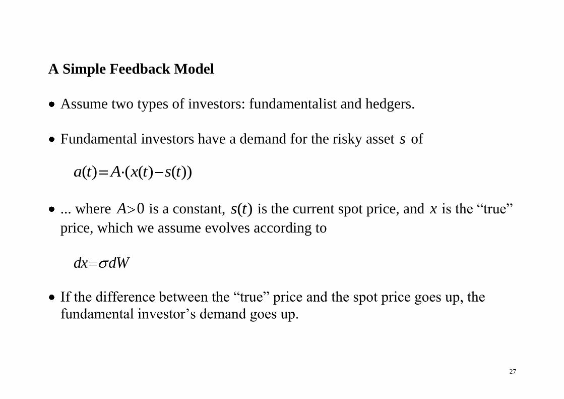
A Simple Feedback Model
Assume two types of investors: fundamentalist and hedgers.
Fundamental investors have a demand for the risky asset s of
( ) ( ( ) ( ))a t A x t s t
... where 0A is a constant, ( )s t is the current spot price, and x is the “true”
price, which we assume evolves according to
dx dW
If the difference between the “true” price and the spot price goes up, the
fundamental investor’s demand goes up.
28
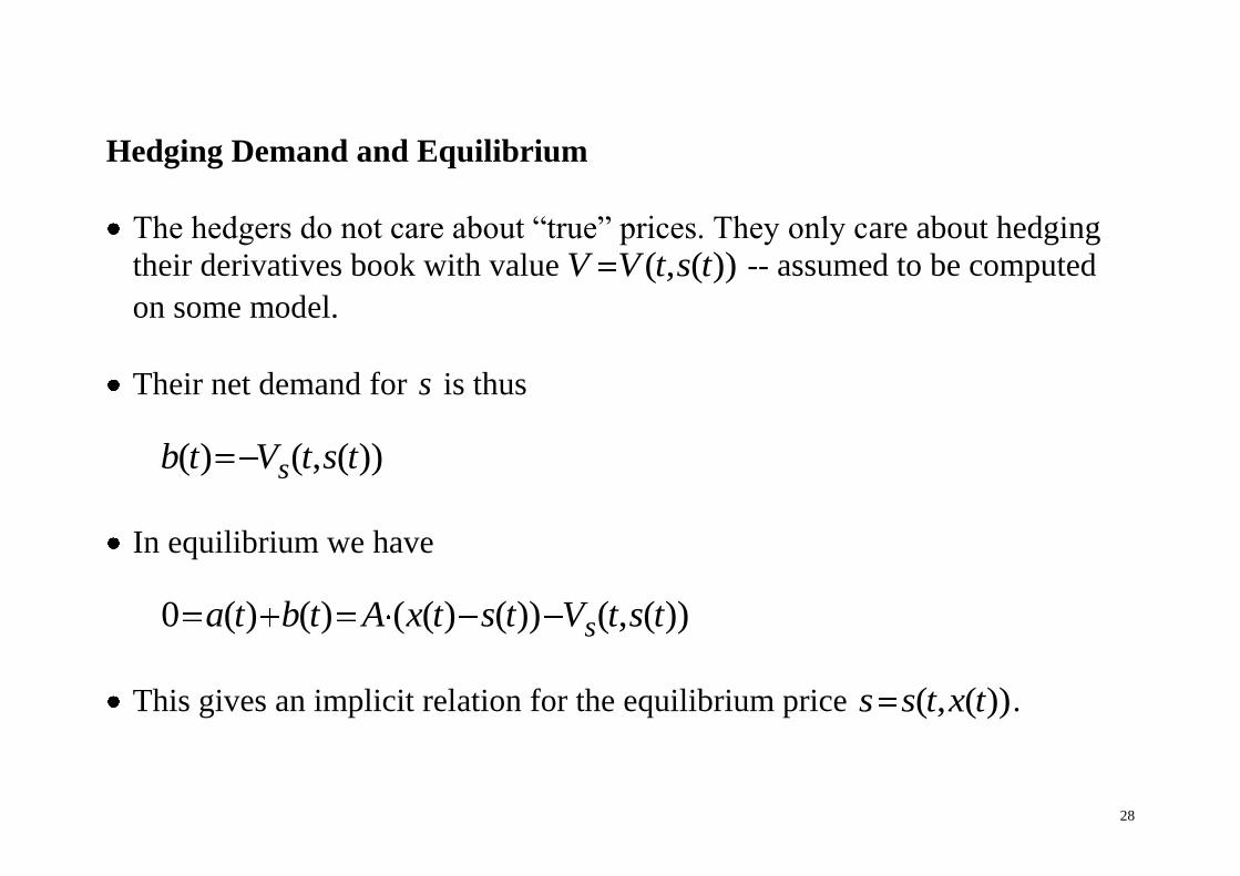
Hedging Demand and Equilibrium
The hedgers do not care about “true” prices. They only care about hedging
their derivatives book with value ( , ( ))V V t s t -- assumed to be computed
on some model.
Their net demand for s is thus
( ) ( , ( ))sb t V t s t
In equilibrium we have
0 ( ) ( ) ( ( ) ( )) ( , ( ))sa t b t A x t s t V t s t
This gives an implicit relation for the equilibrium price ( , ( ))s s t x t .
29
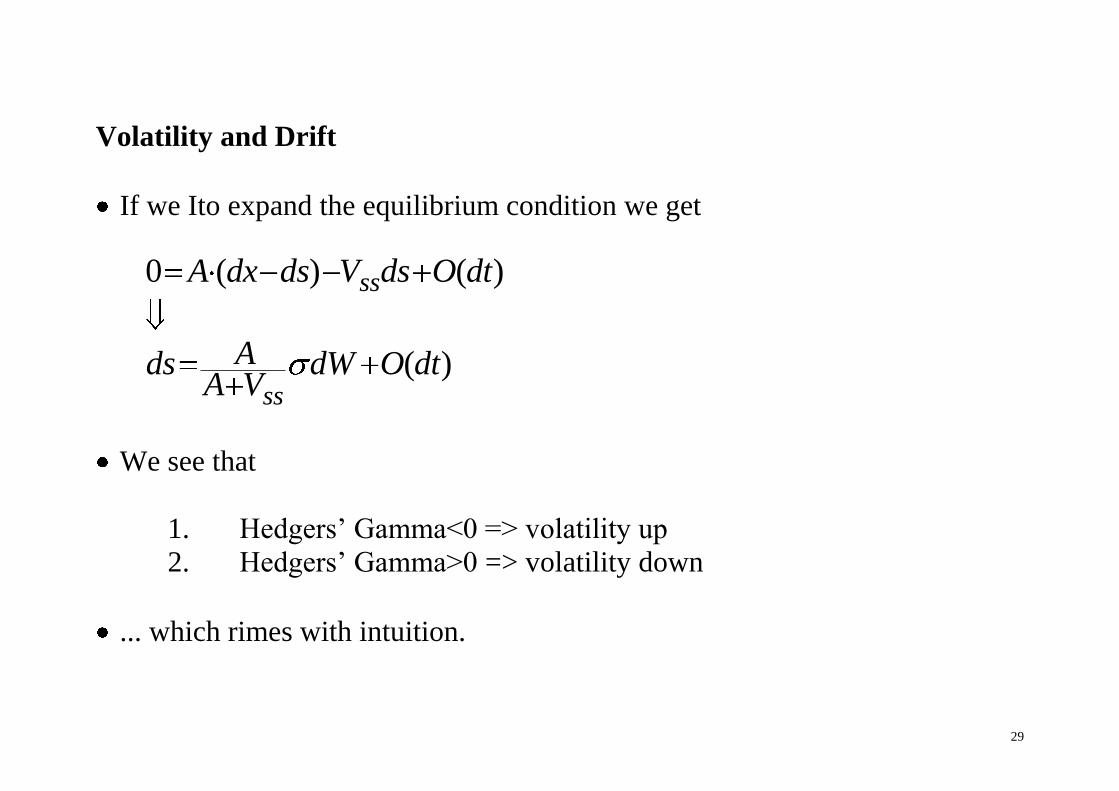
Volatility and Drift
If we Ito expand the equilibrium condition we get
0 ( ) ( )
( )
ss
ss
A dx ds V ds O dt
Ads dW O dtA V
We see that
1. Hedgers’ Gamma<0 => volatility up
2. Hedgers’ Gamma>0 => volatility down
... which rimes with intuition.

30
... and it shows where local volatility can come from.
Model predictions rime with what we saw during the peak of the financial
crisis.
31
The Cause of the Financial Crisis
Did the evil quants and their models and products, cause the financial crisis?
No, the vast majority of bank losses were created the 4000 year old way:
Banks lending money to people who can’t pay back.
Particularly through real estate, examples include:
1. Subprime in the US.
2. Southern Europe.
3. Ireland.
32
In some cases this was facilitated by fancy CDOs, weird models at the rating
agencies, and very non-sceptical attitudes to agency ratings among investors.
Exotic trading books took big hits but generally not of a magnitude that
could impact the solidity of their mother banks.
In most banks the majority of losses came from old fashioned loan books or
from stuff that was kept outside the ordinary trading books and far away
from models.
For example liquidity guarantees to various credit vehicles.
Exotics were not the cause of the financial crisis but they suffered badly
from it because they had many uncovered holes of negative gamma.
Generally speaking: they were actually very poorly hedged.
33
... because the focus had been on pricing rather than hedging.
Anecdote.
34
The Aftermath: 2008-2013
Vanilla derivatives have become exotics.
Dealers can’t lean back on brokers for vanilla quotes.
All market making has to performed with a view.
...and it all requires a modelling effort.
Counterparty credit risk (CVA), funding risk (FVA), market risk (VaR)
impacts have to be priced into all structures.
If XVA is computed correctly it involves simulation of the full client
portfolio.
35
The new exotic are not new payoffs but rather how we discount them.
I.e. how you charge for CVA, DVA, FVA, etc.
Quants used only have exotic traders as their clients – now everyone need
them.
=> More demand for quants than ever!
However, it seems to me that this is not realised everywhere.
Instead, there is a tendency of sitting and dreaming about things returning to
“normal”.
Also, the cost base for most of the big banks is just ridiculous.
36
The Danske Experience
Danske Markets is not an exotic house.
Their main expertise is trading and market making in fixed income: swaps,
bonds, etc.
They’re number one in SEK, NOK, DKK but also very significant presence
in EUR and anything in X-CCY swaps.
Mid 2008, I came to Danske with a small crew with the purpose of
enhancing Danske’s exotics capabilities.
So we started doing a complete derivatives library from scratch: From
vanilla to exotics, SuperFly.
37
This gave us the possibility of including the Libor basis into yield curve
construction from the beginning.
At the time, pretty much all competitors struggled with this. The trouble was
that almost all systems were built without the capability to incorporate a
basis between, say 3m and 6m Libor.
The bigger the bank – the bigger the trouble.
Already in the fall of 2008, we were able to handle this.
Moreover, basing our model on a collection of curves, the notion of a yield
surface was built in from the start.
And it was quick, the model calibrated to around 100 data points in around
0.5 seconds.
38
During the turmoil around and after the Lehman bankruptcy this was a clear
competitive advantage because we could supply our clients with reliable
prices quickly.
This turned out to be very profitable for Danske during 2009.
The competition has gradually caught up but our Yield Surface is still among
the very best in the industry.
This gave the quant team a very strong name within the bank.
We are currently 20+ quants in the team and we have more or less
SuperFly’ed all calculations within Danske Markets -- and beyond.
This includes:
39
1. Yield surfaces generated automatically every 1-5s for 25 ccys.
2. A very sophisticated (and quick) CVA model.
3. Top notch equity and fx options model suite.
4. A pretty good interest rate option model suite.
5. Bond models.
6. Mortgage bond model.
We have managed to apply top-notch mathematical modelling way beyond
the traditional clients (the exotics traders).
We are currently working on a range of quite exciting projects, including:
- Multithreading and AD for CVA.
- What’s my Delta?
- Trading strategies.
- Hedging under transaction costs.
40
Conclusion
Lesson from the 90s: Calibrate!
Lesson from the 00s: Hedge!
Now: more demand than ever for quants!
Overall:
- There is no limit to how complicated and sophisticated mathematics can be
applied to finance.
- If you can make it work on a computer.
- Nobody cares about Greek letters – but everyone loves good numbers.

41
- Stability and reliability: Having a Toyota is better than dreaming of a
Ferrari.
- The prerequisite for that is that you understand the material and the
computer. So...
- Learn something in school. Learn something always and everywhere.
- You’re not in school to pass the exams, you’re there to learn.
- Be critical – not least about yourself.
- Study the original articles instead of the books!
- There is only one good book: Numerical Recipes in C!