A Multi-Factor, Markov Chain Model for Credit Migrations and Credit Spreads

Jason Z. Wei

Rotman School of ManagementUniversity of Toronto105 St. George Street

Toronto, Ontario, CanadaM5S 3E6

Phone: (416) 978-3698E-mail: wei@mgmt.utoronto.ca

Web: http://mgmt.utoronto.ca/~wei

February 21, 2000

The author wishes to acknowledge financial support by the University of Toronto Connaught Fund and the SocialSciences and Humanities Research Council of Canada. He thanks Long Chen for extensive comments and suggestions, andAlan White for discussions. He also would like to thank Dr. Rui Pan for his generous help in obtaining the bond yield data.

A Multi-Factor, Markov Chain Model for Credit Migrations and Credit Spreads

Abstract

This paper develops and implements a multi-factor, Markov chain model for bond rating

migrations and credit spreads. The building blocks are historical transition matrixes and a set of latent

credit cycle variables. The model’s central feature is for transition matrixes to be time-varying, and

driven by rating-specific latent variables which encompass such economic factors as the business

cycle. The paper weaves together the credit risk modeling and the valuation procedures via linking

the observed and risk-neutral transition matrixes by the estimated risk premiums, and allows credit

derivatives to be priced thereof. The main contributions can be summarized as follows. First, the

paper proposes a model for bond rating transitions that incorporates well documented empirical

properties of transition matrixes such as their dependence on business / credit cycles. The model also

allows for inter-rating variations in credit quality changes. Second, unlike many studies which focus

solely on empirical modeling of rating transitions or default rates, this paper shows how the empirical

model can be implemented for actual valuations. Third, the estimation and calibration procedures are

easy to follow and implement. Other than the historical transition matrixes, the only other data

required are bond prices. Preliminary empirical results show, among other things, that allowing for

inter-rating variations in credit quality changes via a multi-variate model can substantially improve

the goodness of fit.

1. Examples include Altman and Kao [1992a], Lucas and Lonski [1992], Carty and Fons [1994], Fons [1994],Belkin, Suchower and Forest, Jr. [1998], Duffee [1998], and Helwege and Turner[1999].

2. Examples here include Jarrow, Lando and Turnbull [1997], Kijima and Komoribayashi [1998], andLando [2000].

3. Examples include Crouhy, Galai and Mark [2000], Gordy [2000], and Lopez and Saidenberg [2000].

1

I. Introduction

Credit risk modeling and credit derivatives valuation have received tremendous attention from both

academics and practitioners in the past several years. The ever increasing sophistication of derivative

instruments, the desire of protection from counter-party losses in major financial fiascos such as the

collapse of the Long Term Capital Management, and the stepping up of regulatory efforts have all

spurred research on credit risk management.

Roughly speaking, there are two related strands of literature. On the one hand, many authors

have modeled and empirically studied default risk and rating migrations.1 On the other hand, some

authors have used various credit risk / rating migration models to value credit derivatives such as

default swaps and yield spread options. 2 Recently, some studies have emerged which compare and

evaluate various credit risk models currently being used in the industry. 3

In a seminal study by Jarrow, Lando and Turnbull [1997] (hereafter, JLT), rating transitions

were modeled as a time-homogenous Markov chain, which means whether a firm’s rating will change

in the next period is not affected by its rating history (hence, Markov), and the probability of changing

from one rating (e.g. AA) to another (e.g. BBB) remains the same over time (hence, time-

homogenous). For valuation purposes, the observed transition matrix (such as those published by

Moody’s and Standard and Poor’s) must be transformed to incorporate risk premium information

embedded in the bond price data. JLT accomplished this by relying on the time-homogeneity and

Markov assumptions, and the additional assumption that the credit risk premiums are time-varying

to reflect the changing credit spreads in corporate bonds. Kijima and Komoribayashi [1998] made

a modification to the JLT framework to perfect the empirical estimation of the model, but their model

retained all the critical assumptions of JLT.

The setup in JLT can be extended in several dimensions. First, as pointed out by the authors

themselves, time-homogeneity is assumed solely for simplicity of estimation. Empirical evidence in

4. Kim [1999], in a short article appearing in a special issue of Risk, proposed a model very similar to that of Belkin, Suchower, and Forest, Jr [1998]. However, he attemped to link some macroeconomic variables to the shifts oftransition probabilities.

2

the Moody’s Special Report [1992] and the Standard and Poor’s Special Report [1998] indicates that

transition probabilities are time-varying, especially for speculative grade bonds. Specifically, Belkin,

Suchower, and Forest, Jr [1998], and Nickell, Perraudin and Varotto [2000] have shown that

probability transition matrixes of bond ratings are dependent on business cycles. Similarly, Helwedge

and Kleiman [1997], and Alessandrini [1999] have shown respectively that default rates and credit

spreads depend on the stage of the business cycle. Second, a time-homogenous setup rules out not

only the dependence on business cycles, but also the possibility that different ratings respond to credit

condition shifts in different rates. Although there is no known empirical study that directly examines

this aspect of credit risk behavior (which itself is another gap in the literature), inter-rating differences

in credit quality changes is indeed a plausible conjecture. In fact, Altman and Kao [1992b] found that,

over time, higher-rating bonds tend to be more stable than lower-rating bonds as far as retaining their

original ratings is concerned. This can be considered as an indirect support for the conjecture. Third,

theoretically, it is not clear why credit risk premiums should change dramatically year by year.

Intuitively, the premium per unit of (default) risk should remain more or less constant (unless

investors’ risk attitude changes), and it is the varying level of (default) risk, or credit cycle, which

leads to the changes in spreads. As Belkin, Suchower and Forest Jr. [1998] reported, defaults are

more likely in economic downturns than in economic booms.

The only known studies which explicitly recognize the impact of business cycles on rating

transitions are by Belkin, Suchower, and Forest, Jr [1998], and Nickell, Perraudin and Varotto

[2000]. Belkin, Suchower, and Forest, Jr [1998] employed a univariate model whereby all ratings

respond to business cycle shifts in the same manner, and they did not deal with estimating matrixes

under the equivalent martingale measure. 4 Nickell, Perraudin and Varotto [2000] proposed an

ordered probit model which allows a transition matrix to be conditioned on the industry, the country

domicile, and the business cycle. Although they require a large quantity of data to estimate reliable

parameters, their approach is conceptually very appealing. Insofar as the reference asset for most

credit derivatives is company / institution specific, the ability to condition a transition matrix on the

industry (to which the company belongs) is definitely desirable. However, since they also need to

3

model the business cycle as a Markov chain, computing multi-period transition matrixes becomes a

very involved process, and as a result, estimating risk premiums (in order to obtain the risk-neutral

matrixes for valuations) can be quite challenging. In addition, for estimation purposes, they need to

assume cross-sectional independence in rating changes.

The objective of the current paper is to build a credit risk model which circumvents the

aforementioned shortcomings and, at the same time, retains the positive features of the existing

models such as the incorporation of credit / business cycles. Specifically, I propose a multi-factor,

Markov chain model for the evolution of credit ratings. The Markov condition is employed to

facilitate estimations. The multi-factor structure will allow the transition matrix to evolve according

to credit cycles, and allow different ratings to respond in a correlated yet different fashion to the same

change in the general economic conditions. In so doing, I will also ensure that the credit risk

premiums are kept constant. The model can then be applied to valuate such credit derivatives as

default swaps and credit spread options.

The rest of the paper is organized in five sections. The next section contains a brief overview

of the time-homogenous Markov chain model. Section III outlines the proposed framework and

estimation procedures. Section IV presents the data. Section V reports and discusses estimation

results based on historical transition matrixes published by Standard and Poor’s. The last section

concludes.

II. Overview of the Time-Homogenous Markov Chain Model

As in JLT [1997], let S be the set of all possible credit states (including default), and i (i = 1, 2, .....,

K) be the index of its elements, where K is the total number of possible states. For example, for a

bond rating system consisting of AAA, AA, A, BBB, BB, B, CCC, and D (default), i 0 [1, 8] and

K = 8. Furthermore, let pij denote the probability of state i transiting to state j. Then, the discrete

time, time-homogenous transition matrix can be represented by

(1) P '

p11 p12 p13 . . . p1K

p21 p22 p23 . . . p2K

..

..

..pK&1,1 pK&1,2 pK&1,3 . . . pK&1,K

0 0 0 . . . 1

,

4

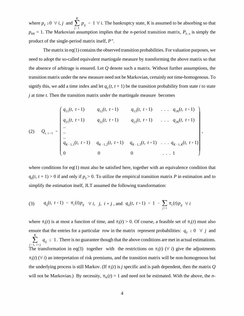
where pij $0 œ i, j and œ i. The bankruptcy state, K is assumed to be absorbing so thatjK

j'1

pij ' 1

pKK = 1. The Markovian assumption implies that the n-period transition matrix, P0, n is simply the

product of the single-period matrix itself, P n.

The matrix in eq(1) contains the observed transition probabilities. For valuation purposes, we

need to adopt the so-called equivalent martingale measure by transforming the above matrix so that

the absence of arbitrage is ensured. Let Q denote such a matrix. Without further assumptions, the

transition matrix under the new measure need not be Markovian, certainly not time-homogenous. To

signify this, we add a time index and let qij (t, t + 1) be the transition probability from state i to state

j at time t. Then the transition matrix under the martingale measure becomes

(2) Qt, t%1 '

q11(t, t%1) q12(t, t%1) q13(t, t%1) . . . q1K(t, t%1)

q21(t, t%1) q22(t, t%1) q23(t, t%1) . . . q2K(t, t%1)......qK&1,1(t, t%1) qK&1,2(t, t%1) qK&1,3(t, t%1) . . . qK&1,K(t, t%1)

0 0 0 . . . 1

,

where conditions for eq(1) must also be satisfied here, together with an equivalence condition that

qij(t, t + 1) > 0 if and only if pij > 0. To utilize the empirical transition matrix P in estimation and to

simplify the estimation itself, JLT assumed the following transformation:

(3) œ i, j, i … j , and œ iqij(t, t%1) ' Bi (t)pij qii(t, t%1) ' 1 & jj… i

Bi(t) pij

where Bi(t) is at most a function of time, and Bi(t) > 0. Of course, a feasible set of Bi(t) must also

ensure that the entries for a particular row in the matrix represent probabilities: qij $ 0 œ j and

There is no guarantee though that the above conditions are met in actual estimations.jK

j'1, i… j

qij # 1.

The transformation in eq(3) together with the restrictions on Bi(t) (œ i) give the adjustments

Bi(t) (œ i) an interpretation of risk premiums, and the transition matrix will be non-homogenous but

the underlying process is still Markov. (If Bi(t) is j specific and is path dependent, then the matrix Q

will not be Markovian.) By necessity, BK(t) = 1 and need not be estimated. With the above, the n-

5

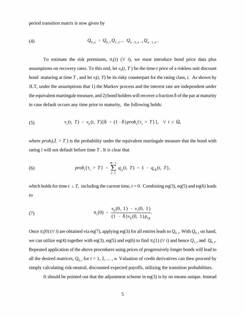
period transition matrix is now given by

(4) Q0, n ' Q0, 1 Q1, 2 ... Qn&2, n&1 Qn&1, n .

To estimate the risk premiums, Bi(t) (œ i), we must introduce bond price data plus

assumptions on recovery rates. To this end, let v0(t, T ) be the time-t price of a riskless unit discount

bond maturing at time T , and let vi(t, T) be its risky counterpart for the rating class, i. As shown by

JLT, under the assumptions that 1) the Markov process and the interest rate are independent under

the equivalent martingale measure, and 2) bond holders will recover a fraction * of the par at maturity

in case default occurs any time prior to maturity, the following holds:

(5) vi (t, T ) ' v0 (t, T ) [* % (1&* ) probt{Ji > T}] , œ i 0 S,

where probt(Ji > T ) is the probability under the equivalent martingale measure that the bond with

rating i will not default before time T . It is clear that

(6) probt{Ji > T} ' jK&1

j'1

qi j(t, T ) ' 1 & qiK(t, T ) ,

which holds for time t # T, including the current time, t = 0. Combining eq(3), eq(5) and eq(6) leads

to

(7) Bi (0) 'v0 (0, 1 ) & vi(0, 1 )

(1 & * )v0 (0, 1) piK

.

Once Bi(0) (œ i) are obtained via eq(7), applying eq(3) for all entries leads to Q0, 1. With Q0, 1 on hand,

we can utilize eq(4) together with eq(3), eq(5) and eq(6) to find Bi(1) (œ i) and hence Q1, 2 and Q0, 2.

Repeated application of the above procedures using prices of progressively longer bonds will lead to

all the desired matrices, Q0, t for t = 1, 2, ... , n. Valuation of credit derivatives can then proceed by

simply calculating risk-neutral, discounted expected payoffs, utilizing the transition probabilities.

It should be pointed out that the adjustment scheme in eq(3) is by no means unique. Instead

5. Note that all entries in the default column must be strictly positive in order for eq(7) to be well defined.Although not explicitly discussed by Kijima and Komoribayashi [1998], their modified procedure of estimating the riskpremiums requires the same condition in order to guarantee the equivalence between the observed probability matrix andthe risk-neutral matrix. To see this, notice from eq(9) that a risk premium is well defined even if piK is zero. In this case, aslong as the risk premium is not exactly 1.0, the corresponding risk-neutral default probability will not be zero, whichviolates the equivalence condition. In this paper, I replace the zero entries in the default column by the smallest non-zeroentry in the transition matrix.

6

of adjusting all entries other than the diagonal entry, Kijima and Komoribayashi [1998] proposed to

adjust all entries other than the default column entry:

(8) œ i, j, j … K , and œ iqij(t, t%1) ' Bi (t)pij qiK(t, t%1) ' 1&jj…K

Bi (t)pij ' 1&Bi(1&piK )

Their procedure leads to the following estimate for the risk premium:

(9) Bi (0) 'vi(0, 1 ) & *v0 (0, 1)

(1 & * ) v0 (0, 1 )1

1 & piK

.

It is apparent that a zero or near-zero default probability would cause the risk premium estimate to

explode in eq(7), but would still lead to a meaningful estimate in eq(9). For this reason, Kijima and

Komoribayashi’s approach will be used in this paper. 5

III. A Multi-Factor Markov Chain Model

To begin with, assume that there exists an average transition matrix similar to the one in eq(1), whose

fixed entries represent average, per-period transition probabilities across all credit cycles. This matrix

can be thought of as a matrix applicable to a typical, average credit condition. Depending on the

condition of the economy for a particular year, the entries will deviate from the averages, and the size

of deviations can be different for different rating categories. In order to facilitate modeling and

estimations, we choose to work with a set of credit variables that drive the time-variations of the

transition probabilities. Thus, we need to define a set of average credit scores which correspond to

the average transition matrix, and model the movement of these credit scores or variables to reflect

the period-specific transition matrixes.

The first step is to devise a mapping through which the average transition probabilities can

be translated into credit scores. To this end, a methodology similar to that of CreditMetricsTM will

7

be adopted. Intuitively, the methodology can be understood as mapping a firm’s future asset returns

to possible ratings, assuming that higher returns correspond to higher ratings, and vice versa.

Inversely, assigning transition probabilities to all other ratings from a given rating is equivalent to

assessing the firm’s asset returns conditional on its current asset return. The mapping may employ

any meaningful statistical distribution, although ease of calculation and estimation may dictate the

choice, given the absence of strong preference for a particular distribution. In this paper, I use the

normal distribution. The detailed procedure is described below.

Since the row sum for any rating in a matrix is always 1.0, we could, for each rating class in

the average transition matrix, construct a sequence of joint bins covering the domain of the normal

variable. This is done by inverting the cumulative normal distribution function starting from the

default column. To illustrate, suppose the firm is currently rated A, and the average probabilities for

A to transit to AAA, AA, A, BBB, BB, B, CCC, and D are 0.0026, 0.0159, 0.8905, 0.0740, 0.0148,

0.0013, 0.0006, and 0.0003 (the sum of which is 1.0). Since the default probability of 0.0003

corresponds to all negative values up to N -1(0.0003) = - 3.432, the first bin is (-4, - 3.432]. Next,

summing 0.0003 and 0.0006 gives us the total probability that the new rating is either CCC or D.

Hence, N -1(0.0009) = - 3.121, and the next bin is (-3.432, -3.121]. By repeating the above, other

bins can be calculated as (-3.121, - 2.848], (-2.848, -2.120], (-2.120, -1.335], (-1.335, 2.086],

(2.086, 2.795], and (2.795, +4). In other words, we could partition the domain of a standard normal

variable by a series of z-scores. An average transition matrix as in eq(1) can then be represented as

(10) Z '

z12 z13 z14 . . . z1K

z22 z23 z24 . . . z2K

..

..

..zK&1,2 zK&1,3 zK&1,4 . . . zK&1,K

.

Notice that the z-score matrix is (K - 1) by (K - 1) because there is no need to convert the row for

the absorbing default state, and because the upper limit of rating AA is the lower limit of rating AAA

which is the highest rating. Obviously, given a z-score matrix, we can also obtain a corresponding

6. Notice that a more general setup such as is in principle the same as thatyij ' "x % $xi % 1 & "2 & $2gijin eq(11). Since x captures the common effect, the two setups imply the same correlation structure. The only difference isthe scaling of xi which has no qualitative consequence anyway.

8

transition matrix.

Once the average credit score matrix is obtained, the next step is to model deviations from

those scores. To this end, it is assumed that the deviations are driven by K mutually independent,

normally distributed factors scaled to standard normal. Without loss of generality, let the first factor

denote the common factor for all ratings, and the rest denote rating-class specific factors. Formally,

generalizing the framework of Belkin, Suchower and Forest Jr. [1998], we define

(11) yij ' " (x % xi) % 1 & 2"2gij , i ' 1, 2, ... , K & 1 , j ' 1, 2, ..., K,

where x is the common factor, xi (i = 1, 2, ..., K - 1) is the rating specific factor, and gij is a non-

systematic, idiosyncratic factor. By assumption, x, xi and gij are i.i.d. standard normal variables, and

the correlation between the aggregate factors of any two rating classes is the same, viz,

corr(yij, yml) = "2 for all i, j, m, and l where i Ö m. For an average year, be definition, the realized

deviations for all rating classes should be close to zero. For each rating or row i, gij (j = 1, 2, ...., K)

represents the idiosyncratic factor. The factors x and xi can be considered as latent variables which

encompass the impacts of all economic variables relevant to rating changes. In this sense, they can

naturally be thought of as credit cycle variables. 6

For a particular year, the realized deviation factor or credit cycle variable in eq(11) is applied

to eq(10), and a transition matrix is then inverted from the adjusted average z-score matrix.

Therefore, the key assumption is the equal magnitude of shifts in z-scores for a particular rating / row.

It is easy to see that, for a given rating, a downward shift in the z-scores leads to an increase in

probabilities of transiting to ratings higher than or equal to the rating in question, and a decrease in

probabilities of transiting to lower ratings / states; and an upward shift in the z-scores leads to the

opposite. For a given row, the deviations of probabilities from the average transition matrix need not

be equal for all columns. In fact, it is almost certain that they are different, given that the shifts in z-

scores are of the same size and that the density function is curved. Here, the unknown shift is

7. The constant risk premiums can also be estimated directly via the observed (as opposed to the fitted) transitionmatrixes. In this case, estimating the parameter "will not be essential. However, the use of fitted matrixes is recommendedsince this will be consistent with the procedure when implying transition matrixes for the future. In addition, by estimatingeq(11) and the z-score deviations, we can study the credit cycle effect, as is done in Section V.

8. To improve the estimation results for each row, I follow Belkin, Suchower, and Forest, Jr [1998] to weigh thesquare of deviations by the inverse of the approximate sample variance of each entry’s probability estimate. In my casethough, the number of observations (i.e. bonds) for each row is irrelevant since it remains constant across columns.Furthermore, unlike Belkin, Suchower, and Forest, Jr [1998], and Kim [1999], I do not scale the adjusted z-score by

because this scaling will lead to the unnatural result that the average z-scores are adjusted /scaled even when1 & 2"2

the shift is zero. Notice also that the above procedure will distort the meaning of the residual term in eq(11). Specifically,there is no guarantee that the sum of the residual is zero as it should be in a usual regression setting. However, this seemsto be a reasonable price to pay, as directly minimizing the sum of squares of z-score deviations leads to very poor fit oftransition matrixes. The poor fit results from the negligence of the highly non-linear relation between z-scores andprobabilities.

9

subtracted from the average z-scores, so that a positive shift means an improvement in credit quality,

and vice versa.

The proposed framework can now be summarized as follows. First, the historical average z-

score matrix and the realized annual z-score matrixes can be fitted into eq(11) to estimate the

parameter, ", and then the annual fitted transition matrixes can be obtained via ". Second, the

constant risk premiums can be estimated using the fitted transition matrixes and historical discount

bond prices. Third, with the constant risk premium estimates and the current prices of discount bonds

of various maturities, the future transition matrixes under the equivalent martingale measure can be

implied, and the valuation of credit derivative securities can then proceed. Detailed estimation

procedures are outlined below. 7

A. Estimating the Factor Realizations and Fitted Transition Matrixes

1) calculate the historical average transition matrix and convert it into a z-score matrix;

2) for each period t, find the shift for each row (of the z-score matrix) to minimize the sum of

deviations of the fitted probabilities from the observed probabilities; this procedure will yield

a time series of z-score deviations for all ratings and all periods, (t = 1, 2, ..., T, and i =)zt, i

1, 2, ..., K - 1); 8

3) calculate the average of the seven shifts for each year, denoted by , which represents theÔ)zt

common / systematic shift;

4) calculate the variance of the time series obtained in Step 3, denoted by Var()z), and compute

the quantity, , which shall be the estimate of ";"̂ ' Var()z)

10

5) for each period t, calculate (since by definition x captures the common shift);Óxt '

Ô)zt /"

6) within the same period t, for each rating class, i, calculate the rating specific deviation as

(in steps 5 and 6, use the estimated " from step 4);xt, i ' () zt, i &Ô)zt) /"

7) obtain the fitted transition matrix for each period by using the average historical matrix and

the z-score adjustments or deviations estimated in Steps 5 and 6 (or simply from Step 2).

(Note: Steps 5 and 6 can be omitted if the values of realized factors are not of interest.)

Notice that, in a univariate model such as that of Belkin, Suchower, and Forest, Jr [1998],

Step 2 is applied to the whole matrix for a particular year to find the common shift, and the parameter

" is estimated in a similar fashion. We could follow this procedure to estimate " first, and then in the

second pass, given the common shift, find the row-specific shifts. In the current paper, I estimate all

quantities in one-pass as outline above, in order to be consistent with the assumption of

independence between x and xi. However, as shown later, the two methods lead to very similar

estimates for ".

B. Estimating the Constant Risk Premiums

Within the proposed framework, the risk premium for each rating class i is assumed to be

constant. Therefore we only need to estimate (K - 1) risk premium parameters. Specifically,

1) for each period t, following Kijima and Komoribayashi [1998], express the probability

transition matrix under the equivalent martingale measure as the risk adjusted, fitted transition

matrix obtained in Procedure A: Q = P(B) (i.e. multiplying the entries of the fitted transition

matrix by the unknown risk premiums while leaving the default column as the adjusting

column to ensure row sum of 1.0);

2) estimate the risk premiums for period t via eq(9). Since bond prices of various maturities are

typically available for each time period, a fitting procedure must be used to estimate the risk

premiums. For the illustrations in Section V, I will only use the one-year bond prices to

estimate the constant risk premiums via minimizing sum of squared deviations between model

prices and observed prices.

C. Estimating Implied Future Transition Matrices Under the Equivalent Martingale Measure

11

Since we do not assume time-homogeneity for the transition matrix, we must estimate or

imply the transition matrix for each of the future periods in order to do valuations. Similar to JLT,

the estimation is recursive: starting from one period out, and successively working out the matrices

for long periods. Specifically,

1) via eq(5), using single period bond prices and an assumed recovery rate to imply the default

probabilities under the equivalent martingale measure for all ratings, q1K (0, 1), q2K (0, 1), ...,

and qK - 1, K (0, 1), as (i = 1, 2, ..., K - 1);v0 (0, 1) & vi (0, 1)

(1 & * ) v0 (0, 1 )2) For each row of the average historical z-score matrix, adjust the z-scores by subtracting

some unknown amount: (i = 1, 2, ...., K - 1);"(x % xi) / ")i

3) for each rating i, we have, by construction,

(where ziK is defined in eq(10)), which leads to an1 & Bi 1 & N [ ( ziK & ")i) ] ' qiK(0, 1 )

estimate for the adjustment:

)i 'ziK & N &1[ 1 & (1 & qiK(0, 1 )) /Bi)

"

(both Bi and " are known by now);

4) repeat Step 3 for each rating / row and complete the adjustment of the z-score matrix;

5) convert the adjusted z-score matrix into a probability transition matrix, and, using the risk

premium estimates, transform this matrix into a matrix that is applicable under the equivalent

martingale measure, Q0, 1 ;

6) multi-period transition matrices are estimated recursively by utilizing eq(4) and bond prices

with successively longer maturities. (Matrix inversion is necessary for the second period and

beyond. For example, once we know and the default column of (calculated usingQ0, 1 Q0, 2

the expression similar to the one in Step 1), we need to invert to obtain the defaultQ0, 1

column of .) Q1, 2

Once the transition matrixes for all future periods are obtained under the equivalent martingale

measure, valuation of credit derivatives such as default swaps can then proceed. The following

section presents estimation results.

12

IV. Data

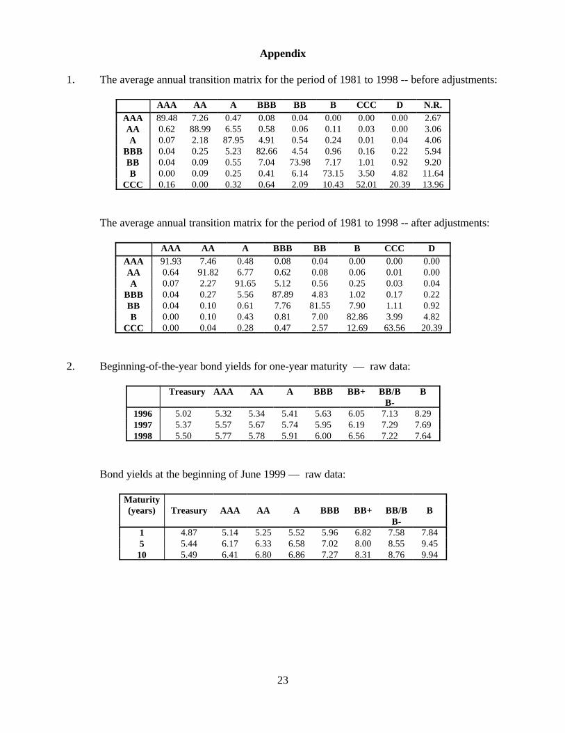
Annual transition matrixes for 1981 - 1998 (inclusive) and the average annual transition matrix

covering the same period are published by Standard & Poor’s [1999]. Weekly treasury and

(industrial) corporate bond yields for various maturities (1, 5, 10, 15, 20, and 25) and ratings (AAA,

AA, A, BBB, BB+, BB/BB-, and B) are obtained from the weekly publication, Credit Week (by

Standard & Poor’s). The starting date of the bond yields publication is March 1996.

Certain issues must be resolved before the data can be used. As for the transition matrixes,

several adjustments are made to smooth the transition probabilities. First of all, the raw matrixes from

Standard & Poor’s contain a column titled “N.R.” — not rated. Following JLT [1997], I simply

redistribute the “N.R.” portion to other ratings on a pro rata basis. Unlike JLT [1997], I leave the

default column unchanged given that the “not rated” bonds are non-defaulting bonds (see discussions

in Standard & Poor’s [1999]). Second, within each row, the probability should decline monotonically

on each side of the diagonal entry. Whenever there is a violation, the entry is set equal to the previous

rating’s entry and the difference is equally distributed among the entries between the diagonal entry

and the entry in question. Third, within each column, the entries on each side of the diagonal entry

should also monotonically decline. To minimize excessive arbitrary adjustments, whenever there is

a violation, I simply swap the entry in question with the previous entry, and adjust the two row’s

diagonal entries to ensure a row sum of 1.0. In certain situations, this swapping may have to be done

in several consecutive turns before the proper ranking is achieved. The default column is kept

unchanged throughout the adjustments. The appendix shows, as an illustration, the original raw

matrix for the average annual transition, and the final matrix with the above adjustments. It is worth

noting that the ranking adjustment is not very frequent in that the original matrixes already satisfy the

conditions most of the time.

As for the bond yields, since we are dealing with annual transition matrixes, they are sampled

only at the beginning of the year for 1996, 1997 and 1998. To imply future matrixes, I use the data

of June 1999, which happens to be the end of the data set. The first three years are used to estimate

the constant risk premiums, and the last year’s bond yields are used to demonstrate how to imply

future transition matrixes. For simplicity, I will use only the one-year-maturity bond yields to estimate

the risk premiums. The bond yields are tabulated in the appendix.

13

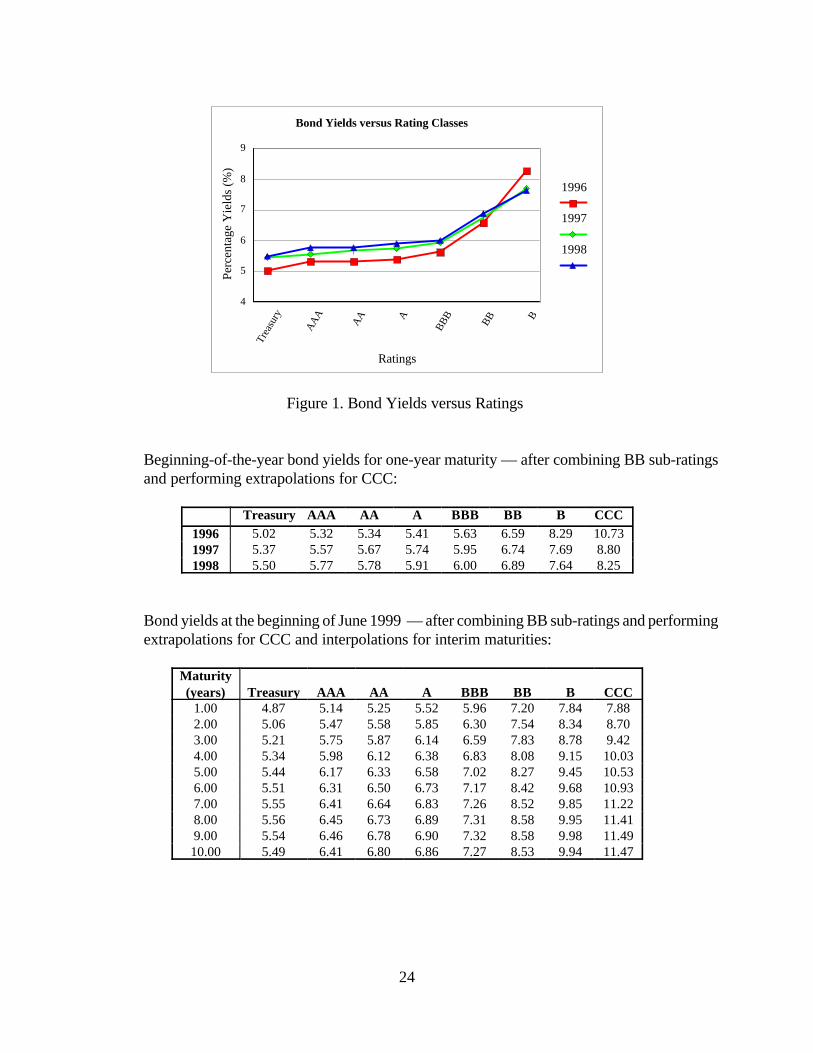
Several issues need to be addressed. First, the corporate bond yields reported in Credit Week

are for industrials, whereas the transition matrixes are based on ratings covering a range of industries

(e.g., industrials, utilities, and financial institutions) in the U.S. and overseas. Notwithstanding the

dominance of U.S. industrials in the rating history (see Nickell, Perraudin and Varotto [2000] for

statistics), the estimation results should be taken with a grain of salt. Second, Credit Week reports

yields separately for BB+ and BB/BB-. I simply use the average of the two yields to proxy the

overall yield for BB. Third, yields for rating CCC are not available. In light of the yield vs. rating

profile depicted in Figure 1 in the appendix, I only use yields for BBB, BB and B to quadratically

extrapolate the yield for rating CCC. Fourth, for 1999, I use the yields of 1-, 5-, and 10-year bonds

to quadratically interpolate the yields for other maturities between 1 and 10 years. Only yields with

maturities up to 5 years are used to demonstrate the estimation in Section V, since most credit

derivatives have a maturity less than five years. The extrapolated / interpolated yields are tabulated

in the appendix. Finally, when implying future transition matrixes beyond one year out, we should use

yields of zero-coupon bonds. Unfortunately, given the lack of information, it is impossible to infer

the pure yield curves from the average yield curves. I simply assume that the reported bond yields are

close approximations for discount bond yields.

V. Estimation Results and Discussions

A. Shifts of Z-Scores and the Fitted Transition Matrixes

By following the estimation procedures outlined in Section III, the parameter " in eq(11) is

estimated to be 0.1116, which indicates that, on average, the correlation between credit migrations

of any two rating classes is about 0.0125. (When the two-pass, sequential procedure is followed, the

estimate for " is 0.1213, very close to the one-pass estimate.) The estimated z-score deviations

(defined as x + xi in eq(11)) are summarized in Table 1. The sample average is -0.016 as opposed to

a theoretical value of zero, and the variance of the average z-score shifts is 1.0 by design. The overall

results are very similar to that of Belkin, Suchower and Forest Jr. [1998]. For example, the 80's saw

predominantly lower than average ratings, while the 90's saw better than average ratings. The year

1990 represents the worst year, while 1996 is the best year, similar to the findings of Belkin,

Suchower and Forest Jr. [1998]. The estimation results are broadly consistent with the empirical

14

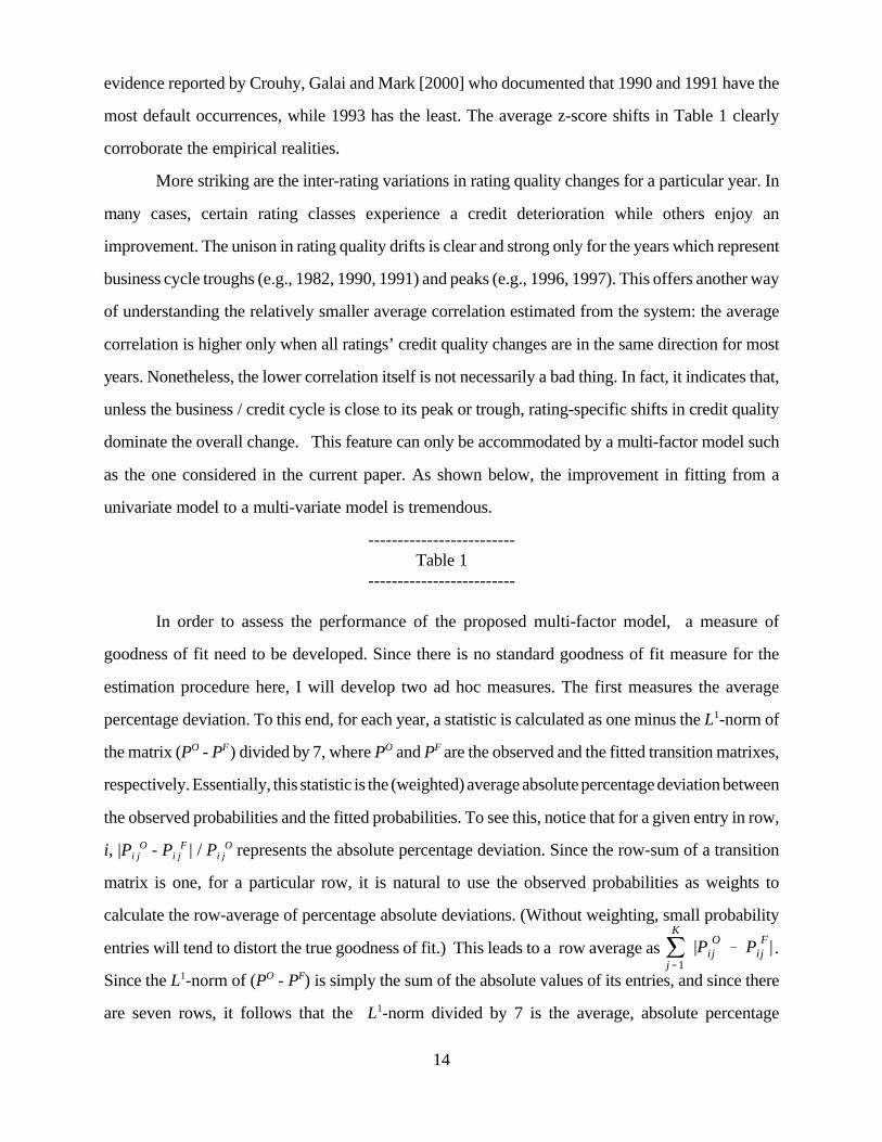
evidence reported by Crouhy, Galai and Mark [2000] who documented that 1990 and 1991 have the

most default occurrences, while 1993 has the least. The average z-score shifts in Table 1 clearly

corroborate the empirical realities.

More striking are the inter-rating variations in rating quality changes for a particular year. In

many cases, certain rating classes experience a credit deterioration while others enjoy an

improvement. The unison in rating quality drifts is clear and strong only for the years which represent

business cycle troughs (e.g., 1982, 1990, 1991) and peaks (e.g., 1996, 1997). This offers another way

of understanding the relatively smaller average correlation estimated from the system: the average

correlation is higher only when all ratings’ credit quality changes are in the same direction for most

years. Nonetheless, the lower correlation itself is not necessarily a bad thing. In fact, it indicates that,

unless the business / credit cycle is close to its peak or trough, rating-specific shifts in credit quality

dominate the overall change. This feature can only be accommodated by a multi-factor model such

as the one considered in the current paper. As shown below, the improvement in fitting from a

univariate model to a multi-variate model is tremendous.

-------------------------Table 1

-------------------------

In order to assess the performance of the proposed multi-factor model, a measure of

goodness of fit need to be developed. Since there is no standard goodness of fit measure for the

estimation procedure here, I will develop two ad hoc measures. The first measures the average

percentage deviation. To this end, for each year, a statistic is calculated as one minus the L1-norm of

the matrix (PO - PF ) divided by 7, where PO and PF are the observed and the fitted transition matrixes,

respectively. Essentially, this statistic is the (weighted) average absolute percentage deviation between

the observed probabilities and the fitted probabilities. To see this, notice that for a given entry in row,

i, |Pi jO - Pi j

F | / Pi jO represents the absolute percentage deviation. Since the row-sum of a transition

matrix is one, for a particular row, it is natural to use the observed probabilities as weights to

calculate the row-average of percentage absolute deviations. (Without weighting, small probability

entries will tend to distort the true goodness of fit.) This leads to a row average as .jK

j'1

|P Oij & P F

ij |

Since the L1-norm of (PO - PF) is simply the sum of the absolute values of its entries, and since there

are seven rows, it follows that the L1-norm divided by 7 is the average, absolute percentage

15

deviation. One minus this quantity represents goodness of fit.

The second measure is similar to an R-square for a regression. Specifically, I calculate the

following statistic,

ji, j, t

(P Oij,t & P avg

i j ) (P Fi j,t & P avg

i j )2

ji, j, t

(P Oij,t & P avg

i j )2ji, j, t

(P Fij, t & P avg

ij )2

where and are defined as before, except for the time index, t. represents a similar entryP Oij, t P F

ij, t P avgij

for the average transition matrix. Given that the mean of both and is zeroP Oij, t & P avg

ij P Fij, t & P avg

ij

by the nature of transition matrixes, the above statistic is indeed the standard definition of R-square

for a linear regression. Since the estimation procedure is slightly different from linear regressions as

discussed in footnote 8, I will call the above statistic a quasi R-square.

The last two columns of Table 1 contain goodness of fit measures. Comparing the multi-

variate model with a univariate model, although the improvement in average percentage deviations

is marginal, the quasi R-square improves substantially, from 0.051 to 0.446, an almost ten-fold

increase. Consistent with the magnitude of ", the large improvement in the quasi R-square indicates

that, it is essential to allow inter-rating variations when modeling rating migrations. Incidentally, for

the multi-variate model, the smallest entry for the first statistic is 0.835 for the year 1981, which

indicates an average percentage deviation of 16.5%. The average across the eighteen years is 0.911,

which indicates an average deviation of 8.9%. For a fitting procedure, this is an encouraging result.

Finally, once the parameter " and the z-score shifts are estimated, a fitted transition matrix

for each year can then be calculated easily. However, those fitted matrixes are only useful for such

purposes as estimating the risk premiums. For brevity, I only report, in Table 2, the fitted matrix for

1998, together with the actual transition matrix for the year and the average annual transition matrix

for the whole sample period.

-------------------------Table 2

-------------------------

B. Risk Premiums

In order to estimate the risk premiums via eq(9), we need to assume a recovery rate and also

16

calculate the bond prices. As shown by JLT [1997] and others, the recover rate depends on the

seniority of the debt and tends to change over time. One can easily make the recovery rate in eq(9)

time- and rating-dependent. However, for illustrative purposes, I simply assume a constant recovery

rate of 0.4, which is the average recovery rate for the period 1974 - 1991 across all ratings (see

Moody’s Special Report [1992]). Moreover, throughout the estimations, bond prices are calculated

by simple discounting:

(12) vi(0, t ) '1

(1 % ri)t

where ri represents the yield for rating class i. The default probabilities are taken from the fitted

transition matrixes. Using fitted transition matrixes for 1996, 1997 and 1998, and the one-year-

maturity bond yields reported in the appendix, the risk premiums are estimated via minimizing the sum

of squared deviations between bond prices based on eq(9) and eq(12). They are reported below.

AAA AA A BBB BB B CCC

0.9959 0.9953 0.9941 0.9932 0.9856 1.0010 1.1210

If we were to plot the risk premiums against the ratings, we would see a skewed U-shaped curve,

with the trough corresponding to rating BB. Interestingly, this is very similar to the results reported

by Kijima and Komoribayashi [1998] who, using a different set of data, estimated the time-varying

risk-premiums for a specific point in time: May 16, 1997. The fact that most of the risk premiums

are close to one implies that the entries of a transition matrix do not change very much when the

change of measure is performed. In contrast, as shown by Kijima and Komoribayashi [1998], the JLT

method of changing measures can cause the probability entries to change significantly.

It is apparent from eq(8) that when the risk premium is exactly unity, the default probability

will remain unchanged when the change of measure is performed, i.e., qiK = piK œ i. A risk premium

smaller than 1.0 means qiK > piK , and vice versa. For higher ratings such as AAA and AA, the

historical default rate is almost zero, but the observed bond prices almost always imply a non-zero

default probability (in the risk-neutral world). In this case, it can be seen from eq(9) that, the

9. Please see Kijima and Komoribayashi [1998], and Lando [2000] for examples of valuing credit derivativesusing risk-neutral transition matrixes.

17

combination of a lower piK and a bigger credit spread (or, equivalently, a smaller value of vi(0, 1) -

*v0(0, 1) > 0) would lead to a smaller estimate of the risk premium. In other words, the smaller risk

premium estimate compensates for the bigger discrepancy between default rates under the physical

world and the risk-neutral world. The opposite analysis holds for risk premiums larger than 1.0. An

implication is that, ideally, the sample period of the bond prices should match that of the historical

transition matrixes to obtain more reliable estimates of risk premiums. Here, we have only three years

of bond price data.

C. Implied Transition Matrixes for Future Periods

Once the risk premiums are available, transition matrixes under the equivalent martingale

measure for any future year can be easily implied from the current prices of zero-coupon bonds.

However, the estimation procedure is recursive if a transition matrix beyond the current year is of

interest. Assuming that the average bond yields tabulated in the appendix are for zero-coupon bonds,

a straightforward application of the procedures outlined in Section III gives us the implied matrixes.

For brevity, I report in Table 3 only the cumulative transition matrixes under the equivalent

martingale measure for years 1, 2, 3, 4 and 5 into the future. These matrixes can then be used to value

credit derivatives. 9

-------------------------Table 3

-------------------------

Notice that the probabilities in the default columns are computed via eq(5) using treasury and

corporate bond yields by assuming a recovery rate of 0.4. The default column, together with the risk

premiums and the average annual transition matrix, determines other entries for the transition

matrixes. It is seen that, for a particular rating, transitions to other ratings, especially the default state,

tend to increase over time. In fact, in a Markov transition framework, all ratings eventually converge

to the absorbing state, which is the default state. It is also interesting to observe the “mean-reverting”

effect in rating changes: ratings A and BBB seem to be the “pulling” states toward which all other

non-default states tend to move. In other words, over time, higher ratings tend to drift downward and

18

lower ratings upward. This same effect has been observed by other authors such as Altman and Kao

[1992b], and Carty and Fons [1994].

Before we conclude, some general discussions are in order. First, although interest rate risk

is not explicitly modeled, the framework in this paper does not require the absence of interest rate

risk. In fact, similar to JLT [1997], as long as the interest rate process and the underlying Markov

process are independent under the equivalent martingale measure, the model applies. However, some

studies have shown that interest rate and credit risk are somewhat related. (See for example,

Longstaff and Schwartz [1995], Duffee [1998], Fridson, Garman and Wu [1997], and Alessandrini

[1999].) Theoretical modeling of the direct relationship between interest rate risk and credit risk is

scanty. General discussions and modeling can be found in JLT [1997] and Jarrow and Turnbull

[2000]. Das and Tufano [1996] ingeniously tackled the problem by modeling a correlation between

the interest rate and the stochastic recovery rate. Building an empirically feasible model with a

correlation between the interest rate and the Markov process will likely require substantial amount

of research. As a starting point, the framework in this paper may be somehow combined with that of

Das and Tufano [1996].

Second, it is known that recovery rate depends on both the rating in question and the stage

of the business cycle (see for example Moody’s Special Report [1992]). The proposed framework

can easily accommodate rating specific, time-varying recovery rates. For estimations, rating specific,

realized historical recovery rates can be used; for implying future transition matrixes, some type of

forecasts would be necessary. Nonetheless, no fundamental modification to the framework is

required.

Third, a normal distribution is assumed for the latent credit variables, which to a large extent

describes reality quite well. Nonetheless, some empirical evidence (e.g. Carty and Leiberman [1997])

suggests that credit migration exhibits memory in its behavior in that a downgrading is more likely

to be followed by another downgrading, and vice versa. Such dynamics imply autoregressive behavior

and would call for ARCH or GARCH type of empirical models. Alternatively, migration memory can

also be modeled by assuming finer partition of credit states as done by Arvanitis, Gregory and Laurent

[1999]. Memories in credit migrations are not allowed in the current framework.

19

Finally, although the framework is based on industry-aggregate transition matrixes, one could

easily modify the estimation procedures to achieve the conditioning effect similar to that in Nickell,

Perraudin and Varotto [2000]. For example, to condition on an industry, one could use the industry

specific bond price data (for all ratings) to estimate the risk premiums and to subsequently imply

transition matrixes for future periods. In this case, the conditioning is achieved through the risk

premium estimations. For valuation purposes, this type of modification is meaningful and sufficient.

As for business cycles, unlike that of Nickell, Perraudin and Varotto [2000], the framework here

does not require an explicit modeling of the business cycle. Future dynamics of business cycles are

fully captured by the observed bond prices used to imply future transition matrixes.

VI. Conclusions

In this paper, I propose a multi-factor Markov chain model for bond rating migrations and credit

spreads. The model takes the historical average transition matrix as the starting point, and allows the

actual realized matrixes to deviate from this average. The deviations are driven by a set of latent,

credit cycle variables which are assumed to be normally distributed. In contrast to most existing

models, the model in this paper allows the transition probabilities to be business cycle dependent.

Using historical transition matrixes and bond prices, the paper shows how to estimate the risk

premiums required to convert transition matrixes from the physical measure to the risk-neutral

measure which can be used to value credit derivatives.

The main advantages of the multi-factor Markov Chain model can be summarized as follows.

First, it allows the rating transition probabilities to be time varying and driven by business cycles. This

is desirable because the time varying nature of transition matrixes and default rates has been

documented by many studies (e.g., Moody’s Special Report [1992], Helwedge and Kleiman [1997],

Belkin, Suchower, and Forest, Jr [1998], Standard and Poor’s Special Report [1998],

Alessandrini [1999], and Nickell, Perraudin and Varotto [2000]).

Second, the model allows different ratings to react differently to the same credit condition

change. For instance, an economic downturn will increase the chance for most bonds to be

downgraded. But conceivably, lower-rated bonds will be more susceptible to the overall credit

deterioration. Meantime, the model also allows the rating shifts to be cross-sectionally correlated,

20

which is again a desirable feature.

Third, unlike most studies on credit risk or credit spreads, the framework in this paper weaves

together credit risk modeling and credit derivatives valuation. It shows how the framework can be

implemented for valuation purposes. This is why it is also a credit spread model.

The estimation results indicate that the overall, average correlation between ratings in credit

quality changes is weak. It is only the business cycle trough and peak years that saw a clear

correlation in that all ratings tend to deteriorate or improve at the same time. For other years, inter-

rating variations in credit quality changes are frequently present. This implies that, although

incorporating the business cycle impact is important in rating migration modeling, it is crucial to allow

inter-rating variations, which can only be achieved by a multi-variate model such as the one

considered in this paper. It is shown that the quasi R-square, as a measurement of goodness of fit,

improves by almost ten folds when a univariate model is replaced by a multi-variate model.

21

References

Alessandrini, F., 1999, Credit Risk, Interest Rate Risk, and the Business Cycle, Journal of FixedIncome, Vol 9, No 2.

Altman, E. I. and D. L. Kao, 1992a, Rating Drift of High Yield Bonds, Journal of Fixed Income, Vol1, No. 4.

Altman, E. I. and D. L. Kao, 1992b, The Implications of Corporate Bond Ratings Drift, Financial

Analyst s Journal, May-June. Arvanitis, A., J. Gregory and J-P Laurent, 1999, Building Models for Credit Spreads, Journal of

Derivatives, Vol 6, No 3.

Belkin, B., S. Suchower, and L. Forest Jr, 1998, A One-Parameter Representation of Credit Risk andTransition Matrices, CreditMetrics® Monitor, Third Quarter, 1998. (http://www.riskmetrics.com/cm/pubs/index.cgi)

Carty, L. V. and J. S. Fons, 1994, Measuring Changes in Corporate Credit Quality, Journal of FixedIncome, June 1994.

Carty,, L. V. and D. Lieberman, 1997, Historical Default Rates of Corporate Bond Issuers 1920-1996, Moody’s Investor Services.

CreditMetricsTM, JP Morgan, http://www.jpmorgan.com/.

Crouhy, M., D. Galai and R. Mark, 2000, A Comparative Analysis of Current Credit Risk Models,Journal of Banking and Finance, Vol 24, No 1/2.

Das, S. and P. Tufano, 1996, Pricing Credit Sensitive Debt When Interest Rates, Credit Ratings andCredit Spreads are Stochastic, Journal of Derivatives, Vol 5, No 2.

Duffee, G., 1998, The Relation between Treasury Yields and Corporate Bond Yield Spreads, Journalof Finance, Vol 53, No 6.

Fons, J. S., 1994, Using Default Rates to Model the Term Structure of Credit Risk, Financial

Analysts Journal, September / October, 1994.

Fridson, M. S., M. C. Garman and S. Wu, 1997, Real Interest Rates and the Default Rate on High-Yield Bonds, Journal of Fixed Income, Vol 7, No 2.

Gordy, M. B., 2000, A Comparative Anatomy of Credit Risk Models, Journal of Banking andFinance, Vol 24, No 1/2.

Helwedge, J. and P. Kleiman, 1997, Understanding Aggregate Default Rates of High-Yield Bonds,Journal of Fixed Income, Vol 7, No 1.

22

Helwege, J and C. M. Turner, 1999, The Slope of the Credit Yield Curve for Speculative-GradeIssuers, Journal of Finance, Vol 54, No 5.

Jarrow, R., D. Lando, and S. Turnbull, 1997, A Markov Model for the Term Structure of Credit RiskSpreads, 1997, Review of Financial Studies, Vol 10, No 2.

Jarrow, R. and S. Turnbull, 2000, The Intersection of Market and Credit Risk, Journal of Bankingand Finance, Vol 24, No ½.

Kijima, M. and K. Komoribayashi, 1998, A Markov Chain Model for Valuing Credit RiskDerivatives, Journal of Derivatives, Fall, 1998.

Kim, J, 1999, Conditioning the Transition Matrix, Credit Risk, a special report by Risk, October,1999.

Lando, D., 2000, Some Elements of Rating-Based Credit Risk Modeling, In: N. Jegadeesh and B.Tuckman (eds): Advanced Fixed-Income Valuation Tools , Wiley, 2000.

Longstaff, F. A. and E. S. Schwartz, 1995, A Simple Approach to Valuing Risky Fixed Floating RateDebt, Journal of Finance, Vol 50, No 3.

Lopez, J. A. and M. R. Saidenberg, 2000, Evaluating Credit Risk Models, Journal of Banking andFinance, Vol 24, No 1/2.

Lucas, D. J. and J. G. Lonski, 1992, Changes in Corporate Credit Quality 1970 - 1990. Vol 1, No4.

Moody’s Special Report, 1992, Corporate Bond Defaults and Default Rates, Moody’s Investors

Services, New York.

Nickell, P., W. Perraudin, and S. Varotto, 2000, Stability of Rating Transitions, Journal of Bankingand Finance, Vol. 24, No. 1/2.

Standard & Poor’s Special Report, 1998, Corporate Defaults Rise Sharply in 1998, Standard &

Poor’s, New York.

Standard & Poor’s, 1999, Rating Performance 1998, Stability & Transition, Standard & Poor’s, NewYork.

23

Appendix

1. The average annual transition matrix for the period of 1981 to 1998 -- before adjustments:

AAA AA A BBB BB B CCC D N.R.AAA 89.48 7.26 0.47 0.08 0.04 0.00 0.00 0.00 2.67AA 0.62 88.99 6.55 0.58 0.06 0.11 0.03 0.00 3.06A 0.07 2.18 87.95 4.91 0.54 0.24 0.01 0.04 4.06

BBB 0.04 0.25 5.23 82.66 4.54 0.96 0.16 0.22 5.94BB 0.04 0.09 0.55 7.04 73.98 7.17 1.01 0.92 9.20B 0.00 0.09 0.25 0.41 6.14 73.15 3.50 4.82 11.64

CCC 0.16 0.00 0.32 0.64 2.09 10.43 52.01 20.39 13.96

The average annual transition matrix for the period of 1981 to 1998 -- after adjustments:

AAA AA A BBB BB B CCC DAAA 91.93 7.46 0.48 0.08 0.04 0.00 0.00 0.00AA 0.64 91.82 6.77 0.62 0.08 0.06 0.01 0.00A 0.07 2.27 91.65 5.12 0.56 0.25 0.03 0.04

BBB 0.04 0.27 5.56 87.89 4.83 1.02 0.17 0.22BB 0.04 0.10 0.61 7.76 81.55 7.90 1.11 0.92B 0.00 0.10 0.43 0.81 7.00 82.86 3.99 4.82

CCC 0.00 0.04 0.28 0.47 2.57 12.69 63.56 20.39

2. Beginning-of-the-year bond yields for one-year maturity — raw data:

Treasury AAA AA A BBB BB+ BB/BB-

B

1996 5.02 5.32 5.34 5.41 5.63 6.05 7.13 8.291997 5.37 5.57 5.67 5.74 5.95 6.19 7.29 7.691998 5.50 5.77 5.78 5.91 6.00 6.56 7.22 7.64

Bond yields at the beginning of June 1999 — raw data:

Maturity(years) Treasury AAA AA A BBB BB+ BB/B

B-B

1 4.87 5.14 5.25 5.52 5.96 6.82 7.58 7.845 5.44 6.17 6.33 6.58 7.02 8.00 8.55 9.45

10 5.49 6.41 6.80 6.86 7.27 8.31 8.76 9.94

24

Trea

sury

AA

A

AA A

BB

B

BB B

Ratings

4

5

6

7

8

9

Perc

enta

ge Y

ield

s (%

)

1996

1997

1998

Bond Yields versus Rating Classes

Figure 1. Bond Yields versus Ratings

Beginning-of-the-year bond yields for one-year maturity — after combining BB sub-ratingsand performing extrapolations for CCC:

Treasury AAA AA A BBB BB B CCC

1996 5.02 5.32 5.34 5.41 5.63 6.59 8.29 10.731997 5.37 5.57 5.67 5.74 5.95 6.74 7.69 8.801998 5.50 5.77 5.78 5.91 6.00 6.89 7.64 8.25

Bond yields at the beginning of June 1999 — after combining BB sub-ratings and performingextrapolations for CCC and interpolations for interim maturities:

Maturity(years) Treasury AAA AA A BBB BB B CCC

1.00 4.87 5.14 5.25 5.52 5.96 7.20 7.84 7.882.00 5.06 5.47 5.58 5.85 6.30 7.54 8.34 8.703.00 5.21 5.75 5.87 6.14 6.59 7.83 8.78 9.424.00 5.34 5.98 6.12 6.38 6.83 8.08 9.15 10.035.00 5.44 6.17 6.33 6.58 7.02 8.27 9.45 10.536.00 5.51 6.31 6.50 6.73 7.17 8.42 9.68 10.937.00 5.55 6.41 6.64 6.83 7.26 8.52 9.85 11.228.00 5.56 6.45 6.73 6.89 7.31 8.58 9.95 11.419.00 5.54 6.46 6.78 6.90 7.32 8.58 9.98 11.4910.00 5.49 6.41 6.80 6.86 7.27 8.53 9.94 11.47

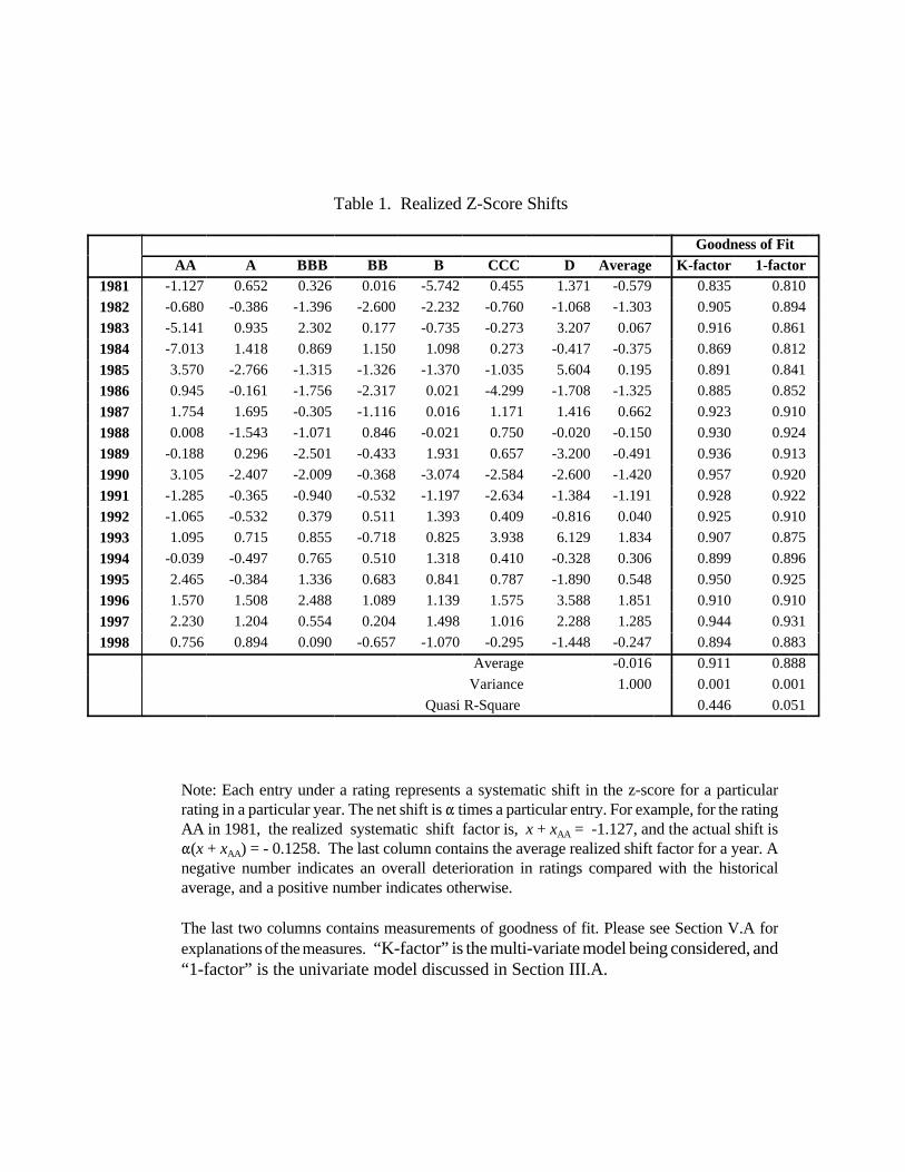
Table 1. Realized Z-Score Shifts

Goodness of Fit AA A BBB BB B CCC D Average K-factor 1-factor

1981 -1.127 0.652 0.326 0.016 -5.742 0.455 1.371 -0.579 0.835 0.810

1982 -0.680 -0.386 -1.396 -2.600 -2.232 -0.760 -1.068 -1.303 0.905 0.894

1983 -5.141 0.935 2.302 0.177 -0.735 -0.273 3.207 0.067 0.916 0.861

1984 -7.013 1.418 0.869 1.150 1.098 0.273 -0.417 -0.375 0.869 0.812

1985 3.570 -2.766 -1.315 -1.326 -1.370 -1.035 5.604 0.195 0.891 0.841

1986 0.945 -0.161 -1.756 -2.317 0.021 -4.299 -1.708 -1.325 0.885 0.852

1987 1.754 1.695 -0.305 -1.116 0.016 1.171 1.416 0.662 0.923 0.910

1988 0.008 -1.543 -1.071 0.846 -0.021 0.750 -0.020 -0.150 0.930 0.924

1989 -0.188 0.296 -2.501 -0.433 1.931 0.657 -3.200 -0.491 0.936 0.913

1990 3.105 -2.407 -2.009 -0.368 -3.074 -2.584 -2.600 -1.420 0.957 0.920

1991 -1.285 -0.365 -0.940 -0.532 -1.197 -2.634 -1.384 -1.191 0.928 0.922

1992 -1.065 -0.532 0.379 0.511 1.393 0.409 -0.816 0.040 0.925 0.910

1993 1.095 0.715 0.855 -0.718 0.825 3.938 6.129 1.834 0.907 0.875

1994 -0.039 -0.497 0.765 0.510 1.318 0.410 -0.328 0.306 0.899 0.896

1995 2.465 -0.384 1.336 0.683 0.841 0.787 -1.890 0.548 0.950 0.925

1996 1.570 1.508 2.488 1.089 1.139 1.575 3.588 1.851 0.910 0.910

1997 2.230 1.204 0.554 0.204 1.498 1.016 2.288 1.285 0.944 0.931

1998 0.756 0.894 0.090 -0.657 -1.070 -0.295 -1.448 -0.247 0.894 0.883

Average -0.016 0.911 0.888

Variance 1.000 0.001 0.001

Quasi R-Square 0.446 0.051

Note: Each entry under a rating represents a systematic shift in the z-score for a particularrating in a particular year. The net shift is " times a particular entry. For example, for the ratingAA in 1981, the realized systematic shift factor is, x + xAA = -1.127, and the actual shift is"(x + xAA) = - 0.1258. The last column contains the average realized shift factor for a year. Anegative number indicates an overall deterioration in ratings compared with the historicalaverage, and a positive number indicates otherwise.

The last two columns contains measurements of goodness of fit. Please see Section V.A forexplanations of the measures. “K-factor” is the multi-variate model being considered, and“1-factor” is the univariate model discussed in Section III.A.

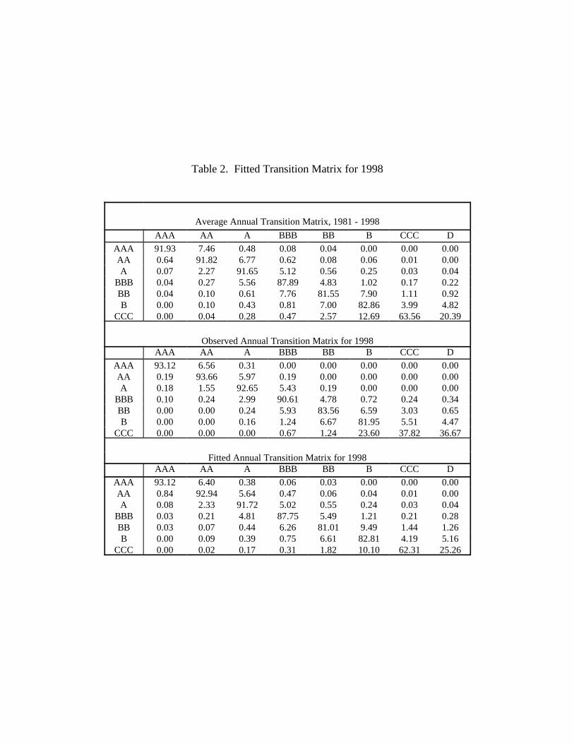
Table 2. Fitted Transition Matrix for 1998

Average Annual Transition Matrix, 1981 - 1998

AAA AA A BBB BB B CCC D

AAA 91.93 7.46 0.48 0.08 0.04 0.00 0.00 0.00AA 0.64 91.82 6.77 0.62 0.08 0.06 0.01 0.00A 0.07 2.27 91.65 5.12 0.56 0.25 0.03 0.04

BBB 0.04 0.27 5.56 87.89 4.83 1.02 0.17 0.22BB 0.04 0.10 0.61 7.76 81.55 7.90 1.11 0.92B 0.00 0.10 0.43 0.81 7.00 82.86 3.99 4.82

CCC 0.00 0.04 0.28 0.47 2.57 12.69 63.56 20.39

Observed Annual Transition Matrix for 1998AAA AA A BBB BB B CCC D

AAA 93.12 6.56 0.31 0.00 0.00 0.00 0.00 0.00AA 0.19 93.66 5.97 0.19 0.00 0.00 0.00 0.00A 0.18 1.55 92.65 5.43 0.19 0.00 0.00 0.00

BBB 0.10 0.24 2.99 90.61 4.78 0.72 0.24 0.34BB 0.00 0.00 0.24 5.93 83.56 6.59 3.03 0.65B 0.00 0.00 0.16 1.24 6.67 81.95 5.51 4.47

CCC 0.00 0.00 0.00 0.67 1.24 23.60 37.82 36.67

Fitted Annual Transition Matrix for 1998AAA AA A BBB BB B CCC D

AAA 93.12 6.40 0.38 0.06 0.03 0.00 0.00 0.00AA 0.84 92.94 5.64 0.47 0.06 0.04 0.01 0.00A 0.08 2.33 91.72 5.02 0.55 0.24 0.03 0.04

BBB 0.03 0.21 4.81 87.75 5.49 1.21 0.21 0.28BB 0.03 0.07 0.44 6.26 81.01 9.49 1.44 1.26B 0.00 0.09 0.39 0.75 6.61 82.81 4.19 5.16

CCC 0.00 0.02 0.17 0.31 1.82 10.10 62.31 25.26

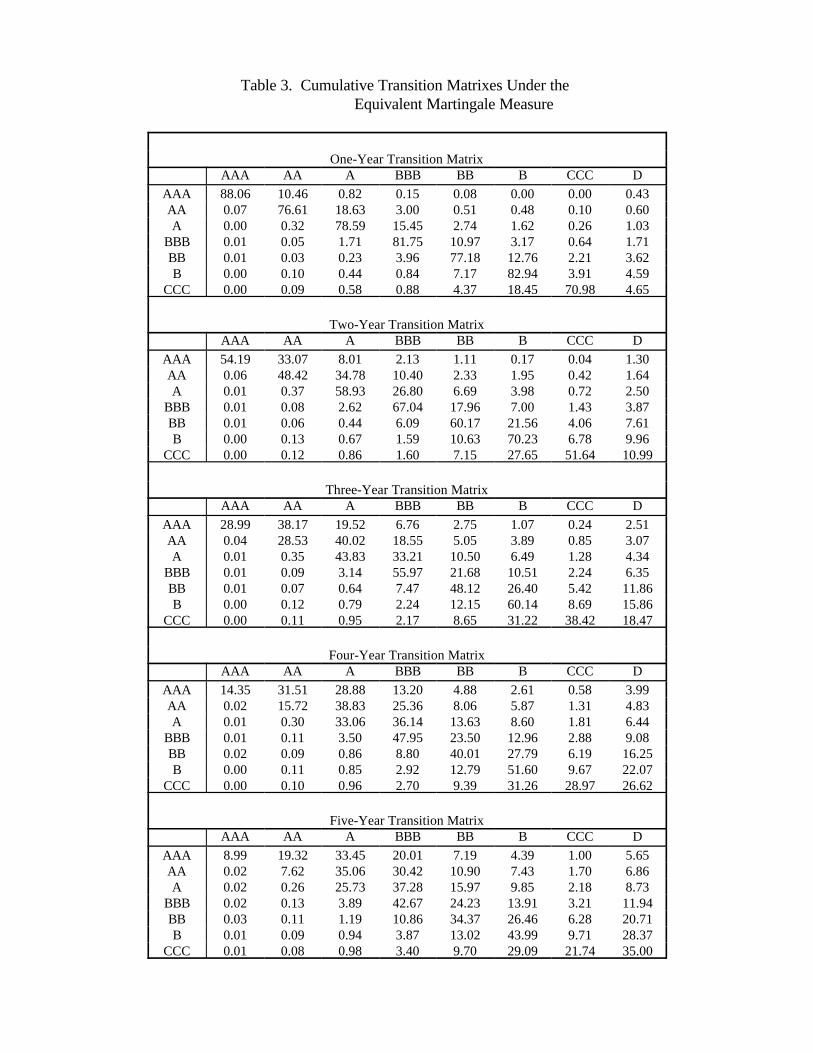
Table 3. Cumulative Transition Matrixes Under the Equivalent Martingale Measure

One-Year Transition MatrixAAA AA A BBB BB B CCC D

AAA 88.06 10.46 0.82 0.15 0.08 0.00 0.00 0.43AA 0.07 76.61 18.63 3.00 0.51 0.48 0.10 0.60A 0.00 0.32 78.59 15.45 2.74 1.62 0.26 1.03

BBB 0.01 0.05 1.71 81.75 10.97 3.17 0.64 1.71BB 0.01 0.03 0.23 3.96 77.18 12.76 2.21 3.62B 0.00 0.10 0.44 0.84 7.17 82.94 3.91 4.59

CCC 0.00 0.09 0.58 0.88 4.37 18.45 70.98 4.65

Two-Year Transition MatrixAAA AA A BBB BB B CCC D

AAA 54.19 33.07 8.01 2.13 1.11 0.17 0.04 1.30AA 0.06 48.42 34.78 10.40 2.33 1.95 0.42 1.64A 0.01 0.37 58.93 26.80 6.69 3.98 0.72 2.50

BBB 0.01 0.08 2.62 67.04 17.96 7.00 1.43 3.87BB 0.01 0.06 0.44 6.09 60.17 21.56 4.06 7.61B 0.00 0.13 0.67 1.59 10.63 70.23 6.78 9.96

CCC 0.00 0.12 0.86 1.60 7.15 27.65 51.64 10.99

Three-Year Transition MatrixAAA AA A BBB BB B CCC D

AAA 28.99 38.17 19.52 6.76 2.75 1.07 0.24 2.51AA 0.04 28.53 40.02 18.55 5.05 3.89 0.85 3.07A 0.01 0.35 43.83 33.21 10.50 6.49 1.28 4.34

BBB 0.01 0.09 3.14 55.97 21.68 10.51 2.24 6.35BB 0.01 0.07 0.64 7.47 48.12 26.40 5.42 11.86B 0.00 0.12 0.79 2.24 12.15 60.14 8.69 15.86

CCC 0.00 0.11 0.95 2.17 8.65 31.22 38.42 18.47

Four-Year Transition MatrixAAA AA A BBB BB B CCC D

AAA 14.35 31.51 28.88 13.20 4.88 2.61 0.58 3.99AA 0.02 15.72 38.83 25.36 8.06 5.87 1.31 4.83A 0.01 0.30 33.06 36.14 13.63 8.60 1.81 6.44

BBB 0.01 0.11 3.50 47.95 23.50 12.96 2.88 9.08BB 0.02 0.09 0.86 8.80 40.01 27.79 6.19 16.25B 0.00 0.11 0.85 2.92 12.79 51.60 9.67 22.07

CCC 0.00 0.10 0.96 2.70 9.39 31.26 28.97 26.62

Five-Year Transition MatrixAAA AA A BBB BB B CCC D

AAA 8.99 19.32 33.45 20.01 7.19 4.39 1.00 5.65AA 0.02 7.62 35.06 30.42 10.90 7.43 1.70 6.86A 0.02 0.26 25.73 37.28 15.97 9.85 2.18 8.73

BBB 0.02 0.13 3.89 42.67 24.23 13.91 3.21 11.94BB 0.03 0.11 1.19 10.86 34.37 26.46 6.28 20.71B 0.01 0.09 0.94 3.87 13.02 43.99 9.71 28.37

CCC 0.01 0.08 0.98 3.40 9.70 29.09 21.74 35.00